Testing High Dimensional Mean Under Sparsity

Abstract Motivated by the likelihood ratio test under the Gaussian assumption, we develop a maximum sum-of-squares test for conducting hypothesis testing on high dimensional mean vector. The proposed test which incorporates the dependence among the variables is designed to ease the computational burden and to maximize the asymptotic power in the likelihood ratio test. A simulation-based approach is developed to approximate the sampling distribution of the test statistic. The validity of the testing procedure is justified under both the null and alternative hypotheses. We further extend the main results to the two sample problem without the equal covariance assumption. Numerical results suggest that the proposed test can be more powerful than some existing alternatives.
Keywords: High dimensionality, Maximum-type-test, Simulation-based approach, Sparsity, Sum-of-squares test

1 Introduction

Due to technology advancement, modern statistical data analysis often deals with high dimensional data arising from many areas such biological studies. High dimensionality poses significant challenge to hypothesis testing. In this paper, we consider a canonical hypothesis testing problem in multivariate analysis, namely inference on mean vector. Let $\{X_{i}\}^{n}_{i=1}$ be a sequence of i.i.d $p$-dimensional random vectors with $\mathbb{E}X_{i}=\theta.$ We are interested in testing

$$H_{0}:\theta=0_{p\times 1}~{}\text{versus}~{}~{}H_{a}:\theta\neq 0_{p\times 1}.$$

When $p\ll n$, the Hotelling’s $T^{2}$ test has been shown to enjoy some optimal properties for testing $H_{0}$ against $H_{a}$ [Anderson (2003)]. However, for large $p$, the finite sample performance of the Hotelling’s $T^{2}$ test is often unsatisfactory. To cope with the high dimensionality, several alternative approaches have been suggested, see e.g Bai and Saranadasa (1996), Srivastava and Du (2008), Srivastava (2009), Chen and Qin (2010), Lopes et al. (2009), Cai et al. (2014), Gregory et al. (2015) and references therein. In general, these tests can be categorized into two types: the sum-of-squares type test and the maximum type test. The former is designed for testing dense but possibly weak signals, i.e., $\theta$ contains a large number of small non-zero entries. The latter is developed for testing sparse signals, i.e., $\theta$ has a small number of large coordinates. In this paper, our interest concerns the case of sparse signals which can arise in many real applications such as detecting disease outbreaks in early stage, anomaly detection in medical imaging [Zhang et al. (2000)] and ultrasonic flaw detection in highly scattering materials [James et al. (2001)].

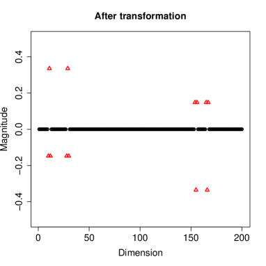
Suitable transformation on the original data, which explores the advantages of the dependence structure among the variables, can lead to magnified signals and thus improves the power of the testing procedure. This phenomenon has been observed in the literature [see e.g. Hall and Jin (2010); Cai et al. (2014); Chen et al. (2014); Li and Zhong (2015)]. To illustrate the point, we consider the signal $\theta=(\theta_{1},\dots,\theta_{200})^{\prime}$, where $\theta$ contains 4 nonzero entries whose magnitudes are all equal to $\psi_{j}\sqrt{\log(200)/100}\approx 0.23\psi_{j}$ with $\psi_{j}$ being independent and identically distributed (i.i.d) random variables such that $P(\psi_{j}=\pm 1)=1/2.$ Let $\Sigma=(\sigma_{i,j})^{p}_{i,j=1}$ with $\sigma_{i,j}=0.6^{|i-j|}$, and $\Gamma=\Sigma^{-1}$. Figure 1 plots the original signal $\theta$ as well as the signal after transformation and studentization $\widetilde{\theta}=(\widetilde{\theta}_{1},\dots,\widetilde{\theta}_{p})^{\prime}$ with $\widetilde{\theta}_{j}=(\Gamma\theta)_{j}/\sqrt{\gamma_{jj}}$. It is clear that the linear transformation magnifies both the strength and the number of signals (the number of nonzero entries increases from 4 to 12 after the linear transformation). In the context of signal recovery, the additional nonzero entries are treated as fake signals and need to be excised, but they are potentially helpful in simultaneous hypothesis testing as they carry certain information about the presence of signal. In general, it appears to be sensible to construct a test based on the transformed data, which targets not only for the largest entry [see Cai et al. (2014)] but also other leading components in $\widetilde{\theta}$. Intuitively such test can be constructed based on $\bar{Z}=\Gamma\bar{X}$ with $\bar{X}=\sum^{n}_{i=1}X_{i}/n$ being the sample mean, which serves as a natural estimator for $\Gamma\theta.$ For known $\Gamma$, a test statistic which examines the largest $k$ components of $\Gamma\theta$ can be defined as,

$$T_{n}(k)=n\max_{1\leq j_{1}<j_{2}<\cdots<j_{k}\leq p}\sum^{k}_{s=1}\frac{\bar{z}_{j_{s}}^{2}}{\gamma_{j_{s},j_{s}}}.$$

Figure 1: Signals before (left panel) and after (right panel) the linear transformation $\Gamma$. The non-zero entries are denoted by $\bigtriangleup$.

If the original mean $\theta$ contains exactly $k$ nonzero components with relatively strong signals, it seems reasonable to expect that $T_{n}(k)$ outperforms $T_{n}(1)$. Interestingly, we shall show that the test statistic $T_{n}(k)$ is closely related with the likelihood ratio (LR) test for testing $H_{0}$ against a sparse alternative on $\theta$.

Our derivation also provides insight on some methods in the literature. In particular, we show that the data transformation based on the precision matrix proposed in Cai et al.(2014) can be derived explicitly using the maximum likelihood principle when $\Theta_{a}$ is the space of vectors with exactly one nonzero component. We also reveal a connection between $T_{n}(k)$ and the thresholding test in Fan (1996).

The rest of the paper is organized as follows. Adopting the maximum likelihood viewpoint, we develop a new class of tests named maximum sum-of-squares tests in Section 2.1. Section 2.2 presents a power analysis. In Section 2.3, we introduce the feasible testing procedure by replacing the precision matrix by its estimator. A simulation-based approach is proposed to approximate the sampling distribution of the test. We describe a modified testing procedure in Section 2.4. Section 2.5 presents some theoretical results based on the Gaussian approximation theory for high dimensional vector. We extend our main results to the two sample problem in Section 3. Section 4 reports some numerical results. Section 5 concludes. The technical details are deferred to the appendix.

Notation. For a vector $a=(a_{1},\dots,a_{p})^{\prime}$ and $q>0$, define $|a|_{q}=(\sum^{p}_{i=1}|a_{i}|^{q})^{1/q}$ and $|a|_{\infty}=\max_{1\leq j\leq p}|a_{j}|$. Set $|\cdot|=|\cdot|_{2}$. Denote by $||\cdot||_{0}$ the $l_{0}$ norm of a vector or the cardinality of a set. For $C=(c_{ij})^{p}_{i,j=1}\in\mathbb{R}^{p\times p}$, define $||C||_{1}=\max_{1\leq j\leq p}\sum^{p}_{i=1}|c_{ij}|$, $||C||_{2}=\max_{|a|=1}|Ca|$ and $||C||_{\infty}=\max_{1\leq i,j\leq p}|c_{ij}|$. Denote by $\text{diag}(C)$ the diagonal matrix $\text{diag}(c_{11},c_{22},\dots,c_{pp})$. The notation $N_{p}(\theta,\Sigma)$ is reserved for the $p$-variate multivariate normal distribution with mean $\theta$ and covariance matrix $\Sigma$.

2 Main results

2.1 Likelihood ratio test

Let $X_{i}=(x_{i1},\dots,x_{ip})^{\prime}$ be a sequence of i.i.d $N_{p}(\theta,\Sigma)$ random vectors with $\Sigma=(\sigma_{ij})^{p}_{i,j=1}$. We are interested in testing

$$H_{0}:\theta\in\Theta_{0}=\{0_{p\times 1}\}\quad\text{versus}\quad H_{a}:\theta\in\Theta_{a}\subseteq\Theta_{0}^{c}.$$ (1)

Let $\Theta_{a,k}=\{b\in\mathbb{R}^{p}:||b||_{0}=k\}$, where $||\cdot||_{0}$ denotes the $l_{0}$ norm of a vector. Notice that $\Theta_{a}\subseteq\Theta_{0}^{c}=\cup_{k=1}^{p}\Theta_{a,k}.$ A practical challenge for conducting high dimensional testing is the specification of the alternative space $\Theta_{a},$ or in another word, the direction of possible violation from the null hypothesis.

Hypothesis testing for high-dimensional mean has received considerable attention in recent literature, see e.g. Srivastava and Du (2008), Srivastava (2009), Chen and Qin (2010), Lopes et al. (2009), Cai et al. (2014), Gregory et al. (2015) among others. Although existing testing procedures are generally designed for a particular type of alternatives, the alternative space is not often clearly specified. In this paper, we shall study (1) with the alternative space $\Theta_{a}$ stated in a more explicit way (to be more precise, it is stated in terms of the $l_{0}$ norm). By doing so, one can derive the test which targets for a particular type of alternative. This formulation also sheds some light on some existing tests. To motivate the subsequent derivations, we consider the following problem

$$H_{0}:\theta\in\Theta_{0}\quad\text{versus}\quad H_{a,k}:\theta\in\Theta_{a,k}.$$ (2)

Given the covariance matrix $\Sigma$ or equivalently the precision matrix $\Gamma=(\gamma_{ij})^{p}_{i,j=1}:=\Sigma^{-1}$, we shall develop a testing procedure based on the maximum likelihood principle. Under the Gaussian assumption, the negative log-likelihood function (up to a constant) is given by

$$l_{n}(\theta)=\frac{1}{2}\sum^{n}_{i=1}(X_{i}-\theta)^{\prime}\Gamma(X_{i}-\theta).$$

The maximum likelihood estimator (MLE) under $H_{a,k}$ is defined as

$$\hat{\theta}=\arg\min_{\theta\in\Theta_{a,k}}\sum^{n}_{i=1}(X_{i}-\theta)^{\prime}\Gamma(X_{i}-\theta).$$ (3)

To illustrate the idea, we first consider the case $\Gamma=I_{p}$, i.e., the components of $X_{i}$ are i.i.d $N(0,1)$. It is straightforward to see that the $k$ nonzero components of $\hat{\theta}$ are equal to $\bar{x}_{j_{s}^{*}}=\sum^{n}_{i=1}x_{ij_{s}^{*}}/n$, where

$$(j_{1}^{*},j_{2}^{*},\dots,j_{k}^{*})=\underset{1\leq j_{1}<j_{2}<\cdots<j_{k}\leq p}{\arg\max}\sum^{k}_{s=1}\bar{x}_{j_{s}}^{2}.$$

Although the maximum is taken over $\binom{n}{k}$ possible sets, it is easy to see that $j_{1}^{*},\dots,j_{k}^{*}$ are just the indices associated with the $k$ largest $|\bar{x}_{j}|$, i.e., we only need to sort $|\bar{x}_{j}|$ and pick the indices associated with the $k$ largest values. In this case, the LR test (with known $\Gamma$) can be written as maximum of sum-of-squares, i.e.,

$$LR_{n}(k)=n\max_{1\leq j_{1}<j_{2}<\cdots<j_{k}\leq p}\sum^{k}_{s=1}\bar{x}_{j_{s}}^{2}.$$

The LR test is seen as a combination of the maximum type test and the sum-of-squares type test and it is designed to optimize the power for testing $H_{0}$ against $H_{a,k}$ with $k\geq 1.$ The two extreme cases are $k=1$ (the sparsest alternative) and $k=p$ (the densest alternative). In the former case, we have $LR_{n}(1)=n|\bar{X}|^{2}_{\infty}=n\max_{1\leq j\leq p}|\bar{x}_{j}|^{2}$, while in the latter case, $LR_{n}(p)=n|\bar{X}|^{2}=n\sum^{p}_{j=1}|\bar{x}_{j}|^{2}$, where $\bar{X}=\sum^{n}_{i=1}X_{i}/n=(\bar{x}_{1},\dots,\bar{x}_{p})^{\prime}$.

We note that an alternative expression for the LR test is given by

$$Thred_{n}(\delta)=n\sum^{p}_{j=1}\bar{x}_{j}^{2}\mathbf{1}\{|\bar{x}_{j}|>\delta\},$$ (4)

for some $\delta>0,$ where $\mathbf{1}\{\cdot\}$ denotes the indicator function. Thus $LR_{n}(k)$ can also be viewed as a thresholding test [see Donoho and Johnstone (1994); Fan (1996)]. In this paper, we focus on the regime of very sparse (e.g. the number of nonzero entries grows slowly with $n$) while strong signals (e.g. the cumulative effect of the nonzero entries of $\theta$ is greater than $\sqrt{2k\log(p)/n}$), and choose $\delta=|\bar{x}_{j_{k+1}^{*}}|$ with $|x_{j_{1}^{*}}|\geq|x_{j_{2}^{*}}|\geq\cdots|x_{j_{p}^{*}}|$ in (4) (assuming that $|x_{j_{k}^{*}}|>|x_{j_{k+1}^{*}}|$). For weaker but denser signals, Fan (1996) suggested the use of $\delta=\sqrt{2\log(pa_{p})/n}$ for $a_{p}=c_{1}(\log p)^{-c_{2}}$ with $c_{1},c_{2}>0.$ A more delicate regime is where the signals are weak so that they cannot have a visible effect on the upper extremes, e.g., the strength of signals is $\sqrt{2r\log(p)/n}$ for $r\in(0,1)$. In this case, the signals and noise may be almost indistinguishable. To tackle this challenging problem, the thresholding test with $\delta=\sqrt{2s\log(p)/n}$ for $s\in(0,1)$ was recently considered in Zhong et al. (2013). And a second level significance test by taking maximum over a range of significance levels (the so-called Higher Criticism test) was used to test the existence of any signals [Donoho and Jin (2004)].

It has been shown in the literature that incorporating the componentwise dependence helps to boost the power of the testing procedure [Hall and Jin (2010); Cai et al. (2014); Chen et al. (2014)]. Below we develop a general test which takes the advantage of the correlation structure contained in $\Gamma.$ We first introduce some notation. For a set $S\subseteq\{1,2,\dots,p\}$, let $\Gamma_{S,S}$ be the submatrix of $\Gamma$ that contains the rows and columns in $S$. Similarly we can define $\Gamma_{S,-S}$ with the rows in $S$ and the columns in $\{1,2,\dots,p\}\setminus S$. Further let $\theta_{S}=(\theta_{j})_{j\in S}$, $\bar{X}_{S}=(\bar{x}_{j})_{j\in S}$ and $\bar{X}_{-S}=(\bar{x}_{j})_{j\in\{1,2,\dots,p\}\setminus S}$. For a set $S$ with $||S||_{0}=k$, we consider the following optimization problem,

$$\max_{\theta\in\mathbb{R}^{p}:\theta_{j}=0,j\notin S}\left(\theta^{\prime}\Gamma\bar{X}-\frac{1}{2}\theta^{\prime}\Gamma\theta\right)=\max_{\theta_{S}\in\mathbb{R}^{k}}\left\{\theta_{S}^{\prime}(\Gamma_{S,S}\bar{X}_{S}+\Gamma_{S,-S}\bar{X}_{-S})-\frac{1}{2}\theta^{\prime}_{S}\Gamma_{S,S}\theta_{S}\right\}.$$

The solution to the above problem is $\theta_{S}=\Gamma_{S,S}^{-1}(\Gamma_{S,S}\bar{X}_{S}+\Gamma_{S,-S}\bar{X}_{-S})$ with the corresponding maximized value equal to $(\Gamma_{S,S}\bar{X}_{S}+\Gamma_{S,-S}\bar{X}_{-S})^{\prime}\Gamma_{S,S}^{-1}(\Gamma_{S,S}\bar{X}_{S}+\Gamma_{S,-S}\bar{X}_{-S})/2$. Based on the above derivation, the LR test for testing $H_{0}$ against $H_{a,k}$ is given by

$$LR_{n}(k)= \max_{\theta\in\Theta_{a,k}}\sum^{n}_{i=1}\left\{X_{i}^{\prime}\Gamma X_{i}-(X_{i}-\theta)^{\prime}\Gamma(X_{i}-\theta)\right\}=2n\max_{\theta\in\Theta_{a,k}}\left(\theta^{\prime}\Gamma\bar{X}-\frac{1}{2}\theta^{\prime}\Gamma\theta\right)$$

$$= 2n\max_{S:||S||_{0}=k}\max_{\theta_{S}\in\mathbb{R}^{k}}\left\{\theta_{S}^{\prime}(\Gamma_{S,S}\bar{X}_{S}+\Gamma_{S,-S}\bar{X}_{-S})-\frac{1}{2}\theta^{\prime}_{S}\Gamma_{S,S}\theta_{S}\right\}$$

$$= n\max_{S:||S||_{0}=k}(\Gamma_{S,S}\bar{X}_{S}+\Gamma_{S,-S}\bar{X}_{-S})^{\prime}\Gamma_{S,S}^{-1}(\Gamma_{S,S}\bar{X}_{S}+\Gamma_{S,-S}\bar{X}_{-S}).$$

Letting $Z=(z_{1},\dots,z_{p})^{\prime}=\Gamma\bar{X}$, a simplified expression is then given by

$$LR_{n}(k)=n\max_{S:||S||_{0}=k}Z_{S}^{\prime}\Gamma_{S,S}^{-1}Z_{S}.$$

It is worth pointing out that $LR_{n}(k)$ is indeed the LR test for testing

$$H_{0}:\theta\in\Theta_{0}\quad\text{against}\quad H_{a,1:k}:\theta\in\cup_{j=1}^{k}\Theta_{a,j},$$

because $\hat{\theta}=\text{argmin}_{\theta\in\cup^{k}_{j=1}\Theta_{a,j}}\sum^{n}_{i=1}(X_{i}-\theta)^{\prime}\Gamma(X_{i}-\theta)=\text{argmin}_{\theta\in\Theta_{a,k}}\sum^{n}_{i=1}(X_{i}-\theta)^{\prime}\Gamma(X_{i}-\theta).$ As an illustration, we consider the following two examples.

Example 2.1 (Sparsest case).

When $k=1$, we have

$$LR_{n}(1)=n\max_{1\leq j\leq p}\frac{|z_{j}|^{2}}{\gamma_{jj}},$$

which has been recently considered in Cai et al. (2014) in the two sample problem. Cai et al. (2014) pointed out that “the linear transformation $\Gamma X_{i}$ magnifies the signals and the number of the signals owing to the dependence in the data”. Although a rigorous theoretical justification was provided in Cai et al. (2014), the linear transformation based on $\Gamma$ still seems somewhat mysterious. Here we “rediscover” the test from a different perspective.

Example 2.2 (Densest case).

To test against the dense alternative $H_{a,p},$ one may consider

$$LR_{n}(p)=n\bar{X}^{\prime}\Gamma\bar{X}=n\sum_{i,j=1}^{p}\bar{x}_{i}\bar{x}_{j}\gamma_{ij},$$

or its $U$-statistic version,

$$LR_{n,U}(p)=\frac{1}{n-1}\sum_{i,j=1}^{p}\gamma_{ij}\sum_{k\neq l}x_{ki}x_{lj}.$$

In view of the results in Chen and Qin (2010), the asymptotic behavior of such test is expected to be very different from $LR_{n}(k)$ with relatively small $k$. A serious investigation for this test is beyond the scope of the current paper.

We note that the test statistic $LR_{n}(k)$ involves taking maximization over $\binom{p}{k}$ tuples $(j_{1},\dots,j_{k})$ with $1\leq j_{1}<\cdots<j_{k}\leq p$, which can be computationally very intensive if $p$ is large. To reduce the computational burden, we consider the following modified test by replacing $\Gamma_{S,S}$ with $\text{diag}(\Gamma_{S,S})$ which contains only the diagonal elements of $\Gamma_{S,S}$. With this substitution, we have

$$T_{n}(k)= n\max_{S:||S||_{0}=k}Z_{S}^{\prime}\text{diag}^{-1}(\Gamma_{S,S})Z_{S}=n\max_{1\leq j_{1}<j_{2}\cdots<j_{k}\leq p}\sum^{k}_{l=1}\frac{|z_{j_{l}}|^{2}}{\gamma_{j_{l},j_{l}}}.$$

To compute the modified statistic, one only needs to sort the values $|z_{j_{l}}|^{2}/\gamma_{j_{l},j_{l}}$ and find the indices corresponding to the $k$ largest ones, say $j_{1}^{*},j_{2}^{*},\dots,j_{k}^{*}$. Then the test statistic can be computed as

$$T_{n}(k)=n\sum^{k}_{l=1}\frac{|z_{j_{l}^{*}}|^{2}}{\gamma_{j_{l}^{*},j_{l}^{*}}}.$$

Therefore, the computation cost for $T_{n}(k)$ with $k>1$ is essentially the same as $LR_{n}(1)$. By the matrix inversion formula $\Gamma_{-j,j}=-\Sigma_{-j,-j}^{-1}\Sigma_{-j,j}\gamma_{jj}$, $z_{j}/\gamma_{jj}=\bar{x}_{j}-\Sigma_{j,-j}\Sigma_{-j,-j}^{-1}\bar{X}_{-j}$. From the above derivation, we note that $n|z_{j}|^{2}/\gamma_{jj}$ can be interpreted as the likelihood ratio test for testing $\theta_{j}=0$ given that $\theta_{k}=0$ for $k\neq j$. This strategy is conceptually simple and can be conveniently implemented in practice. Also it can be generalized to other parametric models.

Remark 2.1.

One may employ the so-called graph-assisted procedure [see e.g. Jin et al. (2014); Ke et al. (2014)] to circumvent the NP hard problem in the definition of $LR_{n}(k)$. Under the Gaussian assumption, $\Gamma$ defines a graph $(V,E)$ in terms of conditional (in)dependence, that is the nodes $i$ and $j$ are connected if and only if $\gamma_{ij}\neq 0.$ Let $J(1),\dots,J(q_{0})$ be all the connected components of $(V,E)$ with size less or equal to $k$. Then an alternative test statistic can be defined as,

$$LR_{graph,n}(k)=n\max\sum^{k_{0}}_{i=1}Z_{J(j_{i})}^{\prime}\Gamma_{J(j_{i}),J(j_{i})}^{-1}Z_{J(j_{i})},$$ (5)

where the maximization is over all $\{j_{1},\dots,j_{k_{0}}\}\subseteq\{1,2,\dots,q_{0}\}$ such that $\sum^{k_{0}}_{i=1}||J(j_{i})||_{0}\leq k.$ Under suitable assumptions on $\Gamma$, it was shown in Jin et al. (2014) that the number of all connected components with size less or equal to $k$ is of the order $O(p)$ (up to a multi-$\log(p)$ term). Greedy algorithm can be used to list all the sub-graphs. Note that $T_{n}(k)$ corresponds to the case where $J(j)=\{j\}$ for $1\leq j\leq p.$ Thus $LR_{graph,n}(k)$ could be viewed as a generalized version of $T_{n}(k)$ with the ability to explore the dependence in $Z$ via the connected components of $(V,E)$.

Remark 2.2.

Another strategy is to use marginal thresholding to screen out a large number of irrelevant variables [see e.g. Fan et al. (2015)]. Specifically, define $\mathcal{M}=\{1\leq j\leq p:|z_{j}|/\sqrt{\gamma_{j,j}}>\delta\}$, where $\delta$ is a proper threshold. A test statistic can be defined as

$$LR_{threshold,n}(k)= n\max_{S\subseteq\mathcal{M}:||S||_{0}=k}Z_{S}^{\prime}\Gamma_{S,S}^{-1}Z_{S},$$

where the optimization can be solved for $\mathcal{M}$ with relatively small size using greedy algorithm.

2.2 Power analysis

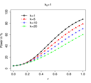
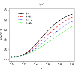
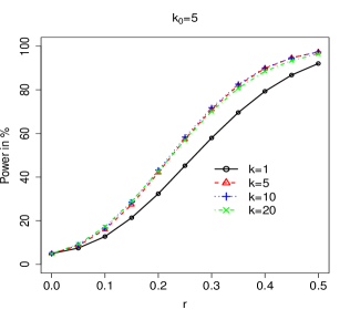
To better understand the power performance of $T_{n}(k)$, we present below a small numerical study. Let $W=(w_{1},w_{2},\dots,w_{p})\sim N_{p}(0,\text{diag}^{-1/2}(\Gamma)\Gamma\text{diag}^{-1/2}(\Gamma))$ and recall that $\widetilde{\theta}=(\widetilde{\theta}_{1},\dots,\widetilde{\theta}_{p})^{\prime}$ with $\widetilde{\theta}_{j}=(\Gamma\theta)_{j}/\sqrt{\gamma_{jj}}$ from the introduction. Define $T^{W}(k;\widetilde{\theta})=\max_{1\leq j_{1}<j_{2}<\cdots j_{k}\leq p}\sum^{k}_{l=1}(w_{j_{l}}+\sqrt{n}\widetilde{\theta}_{j_{l}})^{2}.$ It is obvious that $T_{n}(k)=^{d}T^{W}(k;\widetilde{\theta})$, where “$=^{d}$” means equal in distribution. Denote by $C_{k}(\alpha)$ the $100(1-\alpha)$th quantile of $T^{W}(k;0)$, which can be obtained via simulation (in our study, $C_{k}(\alpha)$ is estimated via $100000$ simulation runs). Define the power function

$$\mathcal{P}(k,\alpha,\widetilde{\theta},\Gamma)=P(T^{W}(k;\widetilde{\theta})>C_{k}(\alpha)).$$

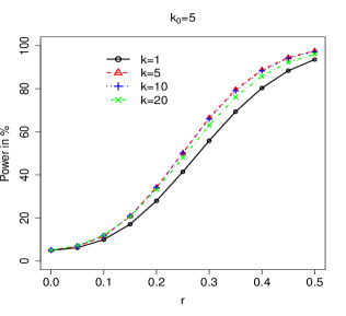
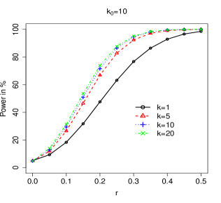
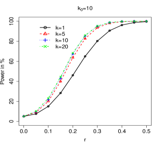
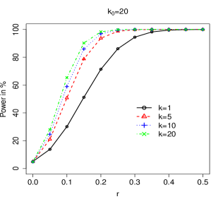
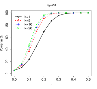
We focus on the AR(1) covariance structure $\Sigma=(\sigma_{i,j})^{p}_{i,j=1}$ with $\sigma_{i,j}=0.6^{|i-j|}$ and $\Gamma=\Sigma^{-1}$. The mean vector $\theta$ is assumed to contain $k_{0}$ nonzero components with the same magnitude $\sqrt{2r\log(p)/n}$, where the locations of the nonzero components are drawn without replacement from $\{1,2,\dots,p\}$. Figure 2 presents the power function $\mathcal{P}(k,0.05,\widetilde{\theta},\Gamma)$ as a curve of $r$ which determines the signal strength, where $k_{0}=1,5,10,20$, and $p=200,1000.$ These results are consistent with our statistical intuition. In particular, for $k_{0}>1$, the power of $T_{n}(k)$ with $k>1$ dominates the power of $T_{n}(1)$. Therefore from the power consideration, when $\theta$ contains more than one nonzero component, it seems beneficial to use $T_{n}(k)$ with $k>1$. This is further confirmed in our simulation studies, see Section 4.

2.3 Feasible test

We have so far focused on the oracle case in which the precision matrix is known. However, in most applications $\Gamma$ is unknown and thus needs to be estimated. Estimating the precision matrix has been extensively studied in the literature in recent years [see e.g. Meinshausen and Bühlmann (2006); Bickel and Levina (2008a; 2008b); Friedman et al. (2008); Yuan (2010); Cai and Liu (2011); Cai et al. (2011); Liu and Wang (2012); Sun and Zhang (2013)].

When $\Gamma$ is known to be banded or bandable, one can employ the banding method based on the cholesky decomposition [Bickel and Levina (2008a)] to estimate $\Gamma$. For sparse precision matrix without knowing the banding structure, the nodewise Lasso and its variants [Meinshausen and Bühlmann (2006); Liu and Wang (2012); Sun and Zhang (2013)] or the constrained $l_{1}$-minimization for inverse matrix estimation (CLIME) [Cai et al. (2011)] can be used to estimate $\Gamma$.

In this paper, we use the nodewise Lasso regression to estimate the precision matrix $\Gamma$ [Meinshausen and Bühlmann (2006)], but other estimation approaches can also be used as long as the resulting estimator satisfies some desired properties [see (8)-(10)]. Let $\widetilde{\mathbf{X}}:=(\widetilde{X}_{1},\widetilde{X}_{2},\dots,\widetilde{X}_{n})^{\prime}\in\mathbb{R}^{n\times p}$ with $\widetilde{X}_{i}=X_{i}-\bar{X}$. Let $\widetilde{\mathbf{X}}_{-j}$ be the $n\times(p-1)$ matrix without the $j$th column. For $j=1,2,\dots,p$, consider

$$\widehat{\gamma}_{j}=\arg\min_{\gamma\in\mathbb{R}^{p-1}}(|\widetilde{X}_{j}-\widetilde{\mathbf{X}}_{-j}\gamma|^{2}/n+2\lambda_{j}|\gamma|_{1}),$$ (6)

with $\lambda_{j}>0$, where $\widehat{\gamma}_{j}=\{\widehat{\gamma}_{jk}:~{}1\leq k\leq p,~{}k\neq j\}$. Let $\widehat{C}=(\widehat{c}_{ij})_{i,j=1}^{p}$ be a $p\times p$ matrix with $\widehat{c}_{ii}=1$ and $\widehat{c}_{ij}=-\widehat{\gamma}_{ij}$ for $i\neq j$. Let $\widehat{\tau}_{j}^{2}=|\widetilde{X}_{j}-\widetilde{\mathbf{X}}_{-j}\widehat{\gamma}_{j}|^{2}/n+\lambda_{j}|\widehat{\gamma}_{j}|_{1}$ and write $\widehat{T}^{2}=\text{diag}(\widehat{\tau}^{2}_{1},\dots,\widehat{\tau}^{2}_{p})$ as a diagonal matrix. The nodewise Lasso estimator for $\Gamma$ is constructed as

$$\widehat{\Gamma}=\widehat{T}^{-2}\widehat{C}.$$

Remark 2.3.

We note that $\widehat{\Gamma}$ does not have to be symmetric. As in Yuan (2010), we can improve them by using a symmetrization step

$$\widetilde{\Gamma}=\underset{A:A=A^{\prime}}{\arg\min}||A-\widehat{\Gamma}||_{1},$$

which can be solved by linear programming. It is obvious that $\widetilde{\Gamma}$ is symmetric, but not guaranteed to be positive-definite. Alternatively, semi-definite programming, which is somewhat more expensive computationally, can be used to produce a nonnegative-definite $\widetilde{\Gamma}$.

Given a suitable precision matrix estimator $\widehat{\Gamma}=(\widehat{\gamma}_{ij})^{p}_{j=1}$ (e.g. obtained via nodewise Lasso), our feasible test can be defined by replacing $\Gamma$ with its estimator, i.e.,

$$T_{fe,n}(k)= n\max_{1\leq j_{1}<j_{2}\cdots<j_{k}\leq p}\sum^{k}_{l=1}\frac{|\widehat{z}_{j_{l}}|^{2}}{\widehat{\gamma}_{j_{l},j_{l}}},$$

where $\widehat{Z}=\widehat{\Gamma}\bar{X}=(\widehat{z}_{1},\dots,\widehat{z}_{p})^{\prime}.$ Under suitable assumptions, it has been shown in Cai et al. (2014) that $T_{fe,n}(1)$ converges to an extreme distribution of Type I. To mimic the sampling distribution of $T_{fe,n}(k)$ for $k\geq 1$ under sparsity assumption, we propose a simulation-based approach which is related with the multiplier bootstrap approach in Chernozhukov et al. (2015). The procedure can be described as follows:

1. Estimate $\Gamma$ by $\widehat{\Gamma}$ using a suitable regularization method.

2. Generate $\widehat{Z}^{*}=(\widehat{z}_{1}^{*},\dots,\widehat{z}_{p}^{*})^{\prime}=\widehat{\Gamma}\sum^{n}_{i=1}(X_{i}-\bar{X})e_{i}/n$, where $e_{i}\sim^{i.i.d}N(0,1)$ are independent of the sample.

3. Compute the simulation-based statistic as

   $$T_{fe,n}^{*}(k)=n\max_{1\leq j_{1}<j_{2}\cdots<j_{k}\leq p}\sum^{k}_{l=1}\frac{|\widehat{z}_{j_{l}}^{*}|^{2}}{\widehat{\gamma}_{j_{l},j_{l}}}.$$

4. Repeat Steps 2-3 several times to get the $1-\alpha$ quantile of $T_{fe,n}^{*}(k),$ which serves as the simulation-based critical value.

2.4 Choice of $k$ and a modified test

In this subsection, we propose a data dependent method for choosing $k$ which is motivated from the power consideration. Consider the Hotelling’s $T^{2}$ test $T^{2}_{n}:=n\bar{X}^{\prime}\widehat{S}^{-1}\bar{X}$ with $\widehat{S}$ being the sample covariance matrix. Bai and Saranadasa (1996) showed that the asymptotic power function for the Hotelling’s $T^{2}$ test under $p/n\rightarrow b\in(0,1)$ has the form

$$\Phi\left(-z_{1-\alpha}+\sqrt{\frac{n(n-p)}{2p}}\theta^{\prime}\Gamma\theta\right),$$ (7)

where $\Phi$ is the distribution function of $N(0,1)$ and $z_{1-\alpha}$ is the $1-\alpha$ quantile of $N(0,1)$. Intuitively, for a set $S$ with $||S||_{0}=k$ and $k<n$, one may expect that the asymptotic power function of $nZ_{S}^{\prime}\Gamma_{S,S}^{-1}Z_{S}$ is determined by the term,

$$\sqrt{\frac{n-k}{2k}}(\Gamma\theta)^{\prime}_{S}\Gamma^{-1}_{S,S}(\Gamma\theta)_{S}.$$

For known $\Gamma$, we note that $Z_{S}^{\prime}\Gamma^{-1}_{S,S}Z_{S}-\frac{k}{n}$ is an unbiased estimator for $(\Gamma\theta)^{\prime}_{S}\Gamma^{-1}_{S,S}(\Gamma\theta)_{S}$. From the power consideration, a natural test statistic can be defined as

$$\max_{1\leq k\leq M}\max_{||S||_{0}=k}\sqrt{\frac{n-k}{2k}}\left(Z_{S}^{\prime}\Gamma^{-1}_{S,S}Z_{S}-\frac{k}{n}\right),$$

where $M$ is an upper bound. By replacing $\Gamma^{-1}_{S,S}$ with $\text{diag}^{-1}(\Gamma_{S,S})$, a computational feasible testing procedure is then given by

$$\widetilde{T}_{n}(M)=\max_{1\leq k\leq M}\max_{||S||_{0}=k}\sqrt{\frac{1-k/n}{2k}}\left(nZ_{S}^{\prime}\text{diag}^{-1}(\Gamma_{S,S})Z_{S}-k\right)=\max_{1\leq k\leq M}\sqrt{\frac{1-k/n}{2k}}\left(T_{n}(k)-k\right).$$

Substituting $\Gamma$ with $\widehat{\Gamma}$, we therefore propose the following test

$$\widetilde{T}_{fe,n}(M)=\max_{1\leq k\leq M}\sqrt{\frac{1-k/n}{2k}}\left(T_{fe,n}(k)-k\right).$$

To approximate its sampling distribution, we suggest the following modified simulation-based statistic in Step 3 above,

$$\widetilde{T}_{fe,n}^{*}(M)=\max_{1\leq k\leq M}\sqrt{\frac{1-k/n}{2k}}\left(n\max_{1\leq j_{1}<j_{2}\cdots<j_{k}\leq p}\sum^{k}_{l=1}\frac{|\widehat{z}_{j_{l}}^{*}|^{2}}{\widehat{\gamma}_{j_{l},j_{l}}}-k\right),$$

where $\widehat{Z}^{*}=(\widehat{z}_{1}^{*},\dots,\widehat{z}_{p}^{*})^{\prime}=\widehat{\Gamma}\sum^{n}_{i=1}(X_{i}-\bar{X})e_{i}/n$ with $e_{i}\sim^{i.i.d}N(0,1)$ that are independent of the sample.

2.5 Theoretical results

In this subsection, we study the theoretical properties of the proposed test and justify the validity of the simulation-based approach. To facilitate the derivations, we make the following assumptions. Denote by $\lambda_{\min}(\Sigma)$ and $\lambda_{\max}(\Sigma)$ the smallest and the largest eigenvalues of $\Sigma$ respectively. Let $d=\max_{1\leq j\leq p}||\{\gamma_{jk}:k\neq j,1\leq k\leq p\}||_{0}$.

Assumption 2.1.

Suppose $\max_{1\leq j\leq p}\sigma_{j,j}<c_{1}$ and $c_{2}<\lambda_{\min}(\Sigma)$ for some $c_{1},c_{2}>0$.

Assumption 2.2.

Suppose $d^{2}\log(p)/n=o(1)$.

Let $\widehat{\Sigma}=\sum^{n}_{i=1}(X_{i}-\bar{X})(X_{i}-\bar{X})^{\prime}/n$. Denote by $\widehat{\Gamma}_{j}$ and $\Gamma_{j}$ the $j$th rows of $\widehat{\Gamma}$ and $\Gamma$ respectively.

Proposition 2.1.

Under Assumptions 2.1-2.2, we have

$$\max_{1\leq j\leq p}|\widehat{\gamma}_{jj}-\gamma_{jj}|=O_{p}\left(\sqrt{\frac{d\log(p)}{n}}\right),$$ (8)

$$\max_{1\leq j\leq p}|\widehat{\Gamma}_{j}-\Gamma_{j}|_{1}=O_{p}\left(d\sqrt{\frac{\log(p)}{n}}\right),$$ (9)

$$||\widehat{\Gamma}\widehat{\Sigma}\widehat{\Gamma}^{\prime}-\widehat{\Gamma}^{\prime}||_{\infty}=O_{p}\left(\sqrt{\frac{d\log(p)}{n}}\right).$$ (10)

By the arguments in the proofs of Lemma 5.3 and Lemma 5.4 in van de Geer et al. (2014), we have (8), (9) and (10) hold if $\widetilde{X}_{i}=X_{i}-\bar{X}$ is replaced by $X_{i}-\theta$ in the nodewise Lasso regression and $\widehat{\Sigma}$ is replaced by $\sum^{n}_{i=1}(X_{i}-\theta)(X_{i}-\theta)^{\prime}/n$. A careful inspection of their proofs shows that the conclusion remains valid when $\theta$ is replaced with $\bar{X}$. We omit the technical details here to conserve space. We are now in position to present the main results in this section. Define the quantity $\phi(\Gamma;k)=\min_{|v|=1,||v||_{0}\leq k}v^{\prime}\Gamma v$. Let $X^{n}_{1}=\{X_{1},\dots,X_{n}\}$.

Theorem 2.1.

Assume that $k^{2}d(\log(np))^{5/2}/\sqrt{n}=o(1)$ and $\phi(\Gamma;k)>c$ for some positive constant $c$. Under Assumptions 2.1-2.2 and $H_{0}$, we have

$$\sup_{t\geq 0}\left|P\left(T_{fe,n}^{*}(k)\leq t\bigg{|}X_{1}^{n}\right)-P\left(T_{fe,n}(k)\leq t\right)\right|=o_{p}(1).$$

Theorem 2.2.

Assume that $M^{4}d(\log(np))^{5/2}/\sqrt{n}=o(1)$ and $\phi(\Gamma;M)>c$ for some positive constant $c$. Under Assumptions 2.1-2.2 with $k$ replaced by $M$ and $H_{0}$, we have

$$\sup_{t_{M}\geq t_{M-1}\geq\cdots\geq t_{1}\geq 0}\left|P\left(\bigcap^{M}_{j=1}\left\{T_{fe,n}^{*}(j)\leq t_{j}\right\}\bigg{|}X_{1}^{n}\right)-P\left(\bigcap^{M}_{j=1}\left\{T_{fe,n}(j)\leq t_{j}\right\}\right)\right|=o_{p}(1).$$

As a consequence, we have

$$\sup_{t\geq 0}\left|P\left(\widetilde{T}_{fe,n}^{*}(M)\leq t\bigg{|}X_{1}^{n}\right)-P\left(\widetilde{T}_{fe,n}(M)\leq t\right)\right|=o_{p}(1).$$

Next we study the power property of the proposed testing procedure. To proceed, we impose the following conditions.

Assumption 2.3.

Assume that $\max_{1\leq j_{1}<j_{2}<\cdots<j_{k}\leq p}\sum^{k}_{l=1}\gamma_{j_{l},j_{l}}\theta_{j_{l}}^{2}\geq(2k+\epsilon)\log(p)/n$ for some $\epsilon>0$.

Assumption 2.4.

Suppose $\sum^{p}_{j=1}I\{\theta_{j}\neq 0\}=p^{r}$ for some $0\leq r<1/4$, and the non-zero locations are randomly uniformly drawn from $\{1,2,\dots,p\}$. And the scheme is independent of $\{X_{i}-\theta\}^{n}_{i=1}$.

Assumption 2.5.

Let $\text{diag}^{-1/2}(\Gamma)\Gamma\text{diag}^{-1/2}(\Gamma)=(\nu_{ij})_{i,j=1}^{p}$. Assume that $\max_{1\leq i<j\leq p}|\nu_{ij}|\leq c_{0}<1$ for some constant $0<c_{0}<1$. Further assume that $\lambda_{\max}(\Sigma)\leq C_{0}$ for some constant $C_{0}>0.$

Define $c^{*}_{\alpha}(k)=\inf\{t>0:P(T_{fe,n}^{*}(k)\leq t|X^{n}_{1})\geq 1-\alpha\}$ and $\widetilde{c}^{*}_{\alpha}(M)=\inf\{t>0:P(\widetilde{T}_{fe,n}^{*}(M)\leq t|X^{n}_{1})\geq 1-\alpha\}$ the simulation-based critical values. The consistency of the testing procedure is established in the following theorem.

Theorem 2.3.

Suppose $k^{2}d(\log(np))^{5/2}/\sqrt{n}=o(1)$. Under Assumptions 2.1-2.5, we have

$$P(T_{fe,n}(k)>c_{\alpha}^{*}(k))\rightarrow 1.$$ (11)

Moreover, suppose Assumption 2.3 holds with $k=M$. Then for $M$ such that $M^{4}d(\log(np))^{5/2}/\sqrt{n}=o(1)$,

$$P(\widetilde{T}_{fe,n}(M)>\widetilde{c}_{\alpha}^{*}(M))\rightarrow 1.$$

When $k=1$, Assumption 2.3 reduces to $\max_{1\leq j\leq p}|\theta_{j}|/\sqrt{\sigma_{jj}}\geq\sqrt{2\{1/(\sigma_{jj}\gamma_{jj})+\epsilon_{0}\}\log(p)/n},$ for some $\epsilon_{0}>0$. According to Theorem 3 of Cai et al. (2014), the separation rate $\sqrt{\log(p)/n}$ is minimax optimal.

Finally, we point out that the Gaussian assumption can be relaxed by employing the recently developed Central Limit Theorem in high dimension [Chernozhukov et al. (2015)]. For a random variable $X$, we define the sub-Gaussian norm [see Definition 5.7 of Vershynin (2012)] as

$$||X||_{\psi}=\sup_{q\geq 1}q^{-1/2}(\mathbb{E}|X|^{q})^{1/q}.$$

Assumption 2.6.

Assume that $\sup_{v\in\mathbb{S}^{p-1}}||v^{\prime}X_{i}||_{\psi}<c_{3}$ and $\sup_{v\in\mathbb{S}^{p-1}}||v^{\prime}\Gamma X_{i}||_{\psi}<c_{4}$ for some constants $c_{3},c_{4}>0$.

Let $W=(w_{1},w_{2},\dots,w_{p})\sim N_{p}(0,\text{diag}^{-1/2}(\Gamma)\Gamma\text{diag}^{-1/2}(\Gamma))$ and define $T^{W}(k)=\max_{1\leq j_{1}<j_{2}<\cdots j_{k}\leq p}\sum^{k}_{l=1}w_{j_{l}}^{2}.$ Specifically we have the following result, which indicates that under the sub-Gaussian assumption, the distribution of $T_{fe,n}(k)$ can be approximated by its Gaussian counterpart $T^{W}(k)$.

Proposition 2.2.

Assume that $d(k\log(np))^{7/2}/\sqrt{n}=o(1)$ and $\phi(\Gamma;k)>c$ for some positive constant $c>0$. Under Assumptions 2.1, 2.2, 2.6 and $H_{0}$, we have

$$\sup_{t\geq 0}\left|P\left(T_{fe,n}(k)\leq t\right)-P\left(T^{W}(k)\leq t\right)\right|=o(1).$$

3 Extension to the two sample problem

3.1 Likelihood ratio test

The maximum likelihood viewpoint allows a direct extension of the above procedure to the two sample problem. Consider two samples $\{X_{i}\}^{n_{1}}_{i=1}\sim^{i.i.d}N_{p}(\theta_{1},\Sigma_{1})$ and $\{Y_{i}\}^{n_{2}}_{i=1}\sim^{i.i.d}N_{p}(\theta_{2},\Sigma_{2})$, where the two samples are independent of each other. A canonical problem in multivariate analysis is the hypothesis testing of

$$H_{0}^{\prime}:\theta_{1}-\theta_{2}\in\Theta_{0}\quad\text{versus}\quad H_{a}^{\prime}:\theta_{1}-\theta_{2}\in\Theta_{a}\subseteq\Theta_{0}^{c}.$$

Given the priori $\theta_{1}-\theta_{2}\in\Theta_{a,k}$, we consider

$$H_{0}^{\prime}:\Delta\in\Theta_{0}\quad\text{versus}\quad H_{a,k}^{\prime}:\Delta\in\Theta_{a,k},$$

where $\Delta=\theta_{1}-\theta_{2}$.

Notation-wise, let $\Gamma_{j}=\Sigma_{j}^{-1}$ for $j=1,2.$ Define $C_{1}=(n_{1}\Gamma_{1}+n_{2}\Gamma_{2})^{-1}n_{1}\Gamma_{1}$ and $C_{2}=(n_{1}\Gamma_{1}+n_{2}\Gamma_{2})^{-1}n_{2}\Gamma_{2}.$ Further let $\Omega^{21}=C_{2}^{\prime}\Gamma_{1}C_{2}$, $\Omega^{12}=C_{1}^{\prime}\Gamma_{2}C_{1}$, $\widetilde{X}=C_{2}^{\prime}\Gamma_{1}(\bar{X}-\widetilde{\theta})$ and $\widetilde{Y}=C_{1}^{\prime}\Gamma_{2}(\bar{Y}-\widetilde{\theta})$, where $\bar{X}=\sum^{n_{1}}_{i=1}X_{i}/n_{1}$, $\bar{Y}=\sum^{n_{2}}_{i=1}Y_{i}/n_{2}$ and

$$\widetilde{\theta}=(n_{1}\Gamma_{1}+n_{2}\Gamma_{2})^{-1}\left(\Gamma_{1}\sum^{n_{1}}_{i=1}X_{i}+\Gamma_{2}\sum^{n_{2}}_{i=1}Y_{i}\right)$$

which is the MLE for $\theta:=\theta_{1}=\theta_{2}$ under the null. The following proposition naturally extends the result in Section 2.1 to the two sample case.

Proposition 3.1.

The LR test for testing $H_{0}^{\prime}$ against $H_{a,k}^{\prime}$ is given by

$$LR_{n}(k)=\max_{S:||S||_{0}=k}(n_{1}\widetilde{X}_{S}-n_{2}\widetilde{Y}_{S})^{\prime}(n_{1}\Omega_{S,S}^{21}+n_{2}\Omega_{S,S}^{12})^{-1}(n_{1}\widetilde{X}_{S}-n_{2}\widetilde{Y}_{S}).$$

3.2 Equal covariance structure

We first consider the case of equal covariance, i.e., $\Gamma:=\Gamma_{1}=\Gamma_{2}$. Simple calculation yields that $C_{1}=n_{1}(n_{1}+n_{2})^{-1}$, $C_{2}=n_{2}(n_{1}+n_{2})^{-1}$, $\widetilde{\theta}=(n_{1}\bar{X}+n_{2}\bar{Y})/(n_{1}+n_{2}),\widetilde{X}=n_{2}^{2}\Gamma(\bar{X}-\bar{Y})/(n_{1}+n_{2})^{2},\widetilde{Y}=n_{1}^{2}\Gamma(\bar{Y}-\bar{X})/(n_{1}+n_{2})^{2}$ and $n_{1}\Omega_{S,S}^{21}+n_{2}\Omega_{S,S}^{12}=n_{1}n_{2}\Gamma/(n_{1}+n_{2}).$ Thus the LR test can be simplified as,

$$LR_{n}(k)=\max_{S:||S||_{0}=k}\frac{n_{1}n_{2}}{n_{1}+n_{2}}(\Gamma\bar{X}-\Gamma\bar{Y})^{\prime}_{S}(\Gamma_{S,S})^{-1}(\Gamma\bar{X}-\Gamma\bar{Y})_{S}.$$ (12)

We note that $LR_{n}(1)$ reduces to the two sample test proposed in Cai et al. (2014). By replacing $\Gamma_{S,S}$ with $\text{diag}(\Gamma_{S,S})$ in (12), we obtain the (infeasible) statistic

$$T_{n}(k)=\max_{1\leq j_{1}<j_{2}<\cdots<j_{k}\leq p}\frac{n_{1}n_{2}}{n_{1}+n_{2}}\frac{(\Gamma\bar{X}-\Gamma\bar{Y})^{2}_{j_{l}}}{\gamma_{j_{l},j_{l}}},$$

which is computationally efficient.

Let $\widehat{\Gamma}=(\widehat{\gamma}_{i,j})^{p}_{i,j=1}$ be a suitable estimator for $\Gamma$ based on the pooled sample. The feasible test is given by

$$T_{fe,n}(k)=\max_{1\leq j_{1}<j_{2}<\cdots<j_{k}\leq p}\frac{n_{1}n_{2}}{n_{1}+n_{2}}\frac{(\widehat{\Gamma}\bar{X}-\widehat{\Gamma}\bar{Y})^{2}_{j_{l}}}{\widehat{\gamma}_{j_{l},j_{l}}}.$$

To approximate the sampling distribution of the above test, one can employ the simulation-based approach described below:

1. Estimate $\widehat{\Gamma}$ using suitable regularization method based on the pooled sample.

2. Let $X^{*}=\sum^{n_{1}}_{i=1}(X_{i}-\bar{X})e_{i}/n_{1}$ and $Y^{*}=\sum^{n_{2}}_{i=1}(Y_{i}-\bar{Y})\tilde{e}_{i}/n_{1}$, where $\{e_{i}\}$ and $\{\tilde{e}_{i}\}$ are two independent sequences of i.i.d $N(0,1)$ random variables that are independent of the sample.

3. Compute the simulation-based statistic $T_{fe,n}^{*}(k)$ by replacing $\bar{X}$ and $\bar{Y}$ with $X^{*}$ and $Y^{*}$.

4. Repeat Steps 2-3 several times to get the $1-\alpha$ quantile of $T_{fe,n}^{*}(k)$, which serves as the simulation-based critical value.

Next, we briefly discuss the choice of $k$. By Theorem 2.1 in Bai and Saranadasa (1996), we know that the asymptotic power function for the two sample Hotelling’s $T^{2}$ test is given by

$$\Phi\left(-z_{1-\alpha}+\sqrt{\frac{N(N-p)}{2p}}\frac{n_{1}n_{2}}{N^{2}}(\theta_{1}-\theta_{2})^{\prime}\Gamma(\theta_{1}-\theta_{2})\right),$$

under $p/N\rightarrow b\in(0,1)$, where $N=n_{1}+n_{2}-2$. Thus for $k<N$, the asymptotic power of $T_{fe,n}(k)$ is related to

$$\sqrt{\frac{N-k}{2k}}\max_{||S||_{0}=k}\{\widehat{\Gamma}(\theta_{1}-\theta_{2})\}^{\prime}_{S}\text{diag}^{-1}(\widehat{\Gamma}_{S,S})\{\widehat{\Gamma}(\theta_{1}-\theta_{2})\}_{S}.$$

Notice that

$$(\Gamma\bar{X}-\Gamma\bar{Y})^{\prime}_{S}\text{diag}^{-1}(\Gamma_{S,S})(\Gamma\bar{X}-\Gamma\bar{Y})_{S}-\frac{k(n_{1}+n_{2})}{n_{1}n_{2}}$$

is an unbiased estimator for $\{\Gamma(\theta_{1}-\theta_{2})\}^{\prime}_{S}\text{diag}^{-1}(\Gamma_{S,S})\{\Gamma(\theta_{1}-\theta_{2})\}_{S}$. Thus we propose to choose $k$ by

$$\widehat{k}= \arg\max_{1\leq k\leq M^{\prime}}\sqrt{\frac{N-k}{2k}}\left(T_{fe,n}(k)-k\right),$$

where $M^{\prime}$ is a pre-specified upper bound for $k$. Following the same spirit in Section 2.4, a modified test statistic is given by

$$\widetilde{T}_{fe,n}(k)=\max_{1\leq k\leq M^{\prime}}\sqrt{\frac{1-k/N}{2k}}\left(\max_{1\leq j_{1}<j_{2}<\cdots<j_{k}\leq p}\frac{n_{1}n_{2}}{n_{1}+n_{2}}\frac{(\widehat{\Gamma}\bar{X}-\widehat{\Gamma}\bar{Y})^{2}_{j_{l}}}{\widehat{\gamma}_{j_{l},j_{l}}}-k\right),$$

and the simulation-based procedure can be used to approximate its sampling distribution.

We can justify the validity of the testing procedure under both the null and alternative hypotheses. The arguments are similar to those in the one sample case, see Sections 2.3 and 6.2.

3.3 Unequal covariance structures

In the case of unequal covariance structures i.e., $\Gamma_{1}\neq\Gamma_{2}$, we cannot use the pooled sample to estimate the covariance structures. Let $\widehat{\Gamma}_{i}$ with $i=1,2$ be suitable precision matrix estimators based on each sample separately. Denote by $\widehat{C}_{i}$ the estimator for $C_{i}$ with $i=1,2$. A particular choice here is given by

$$\widehat{C}_{1}=(n_{1}\widehat{\Gamma}_{1}+n_{2}\widehat{\Gamma}_{2})^{-1}n_{1}\widehat{\Gamma}_{1},\quad\widehat{C}_{2}=(n_{1}\widehat{\Gamma}_{1}+n_{2}\widehat{\Gamma}_{2})^{-1}n_{2}\widehat{\Gamma}_{2}.$$

Further define $\widehat{\Omega}^{21}=\widehat{C}_{2}^{\prime}\widehat{\Gamma}_{1}\widehat{C}_{2}$, $\widehat{\Omega}^{12}=\widehat{C}_{1}^{\prime}\widehat{\Gamma}_{2}\widehat{C}_{1}$, $\widehat{X}=\widehat{C}_{2}^{\prime}\widehat{\Gamma}_{1}(\bar{X}-\widehat{\theta})$ and $\widehat{Y}=\widehat{C}_{1}^{\prime}\widehat{\Gamma}_{2}(\bar{Y}-\widehat{\theta})$, where

$$\widehat{\theta}=\widehat{C}_{1}\bar{X}+\widehat{C}_{2}\bar{Y}.$$

Let $\widehat{\Psi}=(\widehat{\psi}_{ij})_{i,j=1}^{p}=n_{1}\widehat{\Omega}^{21}+n_{2}\widehat{\Omega}^{12}$, and $\widehat{G}=(\widehat{g}_{1},\dots,\widehat{g}_{p})^{\prime}=n_{1}\widehat{X}-n_{2}\widehat{Y}$. By replacing $\widehat{\Psi}$ with $\text{diag}(\widehat{\Psi})$, we suggest the following computational feasible test,

$$T_{fe,n}(k)=\max_{1\leq j_{1}<j_{2}<\cdots<j_{k}\leq p}\sum^{k}_{l=1}\frac{|\widehat{g}_{j_{l}}|^{2}}{\widehat{\psi}_{j_{l},j_{l}}}.$$ (13)

When $k=1$, we have

$$T_{fe,n}(1)=\max_{1\leq j\leq p}\frac{|\widehat{g}_{j}|^{2}}{\widehat{\psi}_{jj}},$$ (14)

which can be viewed as an extension of Cal et al. (2014)’s test statistic to the case of unequal covariances. Again one can employ the simulation-based approach to obtain the critical values for $T_{fe,n}(k)$. In this case, a modified test can be defined in a similar manner as

$$\widetilde{T}_{fe,n}(k)=\max_{1\leq k\leq M^{\prime\prime}}\sqrt{\frac{1-k/N}{2k}}\left(\max_{1\leq j_{1}<j_{2}<\cdots<j_{k}\leq p}\sum^{k}_{l=1}\frac{|\widehat{g}_{j_{l}}|^{2}}{\widehat{\psi}_{j_{l},j_{l}}}-k\right)$$

for some upper bound $M^{\prime\prime}$.

4 Simulation studies

4.1 Empirical size and power

In this section, we report the numerical results for comparing the proposed testing procedure with some existing alternatives. Specially we focus on the two sample problem for testing $H_{0}^{\prime}:\Delta\in\Theta_{0}$ against the alternatives $H_{a,k}^{\prime}:\Delta\in\Theta_{a,k}$. Without loss of generality, we set ${\theta}_{2}={0}$. Note that under $H_{a,k}^{\prime}$, ${\theta}_{1}$ has $k$ non-zero elements. Denote by $\lfloor x\rfloor$ the largest integer not greater than $x$. We consider the settings below.

• Case 1: $k=\lfloor 0.05p\rfloor$ and the non-zero entries are equal to $\varphi_{j}\sqrt{\log(p)/n}$, where $\varphi_{j}$ are i.i.d random variables with $P(\varphi_{j}=\pm 1)=1/2$.

• Case 2: $k=\lfloor\sqrt{p}\rfloor$ and the strength of the signals is the same as (1).

• Case 3: $k=\lfloor p^{0.3}\rfloor$ and the nonzero entries are all equal to $\sqrt{4r\log p/n}$ with $r=0.1,0.2,0.3,0.4,$ and $0.5.$

Here the locations of the nonzero entries are drawn without replacement from $\{1,2,\dots,p\}$. Following Cai et al. (2014), the following four covariance structures are considered.

• (block diagonal ${\Sigma}$): ${\Sigma}=\left(\sigma_{j,k}\right)$  where $\sigma_{j,j}=1$  and $\sigma_{j,k}=0.8$  for $2(r-1)+1\leq j\neq k\leq 2r$,  where $r=1,\ldots,\lfloor p/2\rfloor$ and $\sigma_{j,k}=0$  otherwise.

• (‘bandable’ ${\Sigma}$): ${\Sigma}=\left(\sigma_{j,k}\right)$  where $\sigma_{j,k}=0.6^{|j-k|}$  for $1\leq j,k\leq p$.

• (banded ${\Gamma}$): ${\Gamma}=\left(\gamma_{j,k}\right)$  where $\gamma_{j,j}=2$  for  $j=1,\ldots,p$,  $\gamma_{j,(j+1)}=0.8$  for  $j=1,\ldots,p-1$,  $\gamma_{j,(j+2)}=0.4$  for  $j=1,\ldots,p-2$,  $\gamma_{j,(j+3)}=0.4$  for  $j=1,\ldots,p-3$,  $\gamma_{j,(j+4)}=0.2$  for  $j=1,\ldots,p-4$,  $\gamma_{j,k}=\gamma_{k,j}$  for  $j,k=1,\ldots,p$,  and  $\gamma_{j,k}=0$  otherwise.

• (block diagonal $\Gamma$): Denote by $D$ a diagonal matrix with diagonal elements generated independently from the uniform distribution on $(1,3)$. Let $\Sigma_{0}$ be generated according to (a). Define $\Gamma=D^{1/2}\Sigma^{2}_{0}D^{1/2}$ and $\Sigma=\Gamma^{-1}$.

For each covariance structure, two independent random samples are generated with the same sample size $n_{1}=n_{2}=80$ from the following multivariate models,

$$X=\theta_{1}+\Sigma^{1/2}U_{1},\quad Y=\theta_{2}+\Sigma^{1/2}U_{2},$$ (15)

where $U_{1}$ and $U_{2}$ are two independent $p$-dimensional random vectors with independent components such that $\mathbb{E}(U_{j})=0$ and ${\mbox{var}}(U_{j})=I_{p}$ for $j=1,2$. We consider two cases: $U_{j}\sim N(0,I_{p})$, and the component of $U_{j}$ is standardized Gamma(4,1) random variable such that it has zero mean and unit variance. The dimension $p$ is equal to $50,100$ or $200$. Throughout the simulations, the empirical sizes and powers are calculated based on 1000 Monte Carlo replications.

To estimate the precision matrix, we use the nodewise square root Lasso [Belloni et al. (2012)] proposed in Liu and Wang (2012), which is essentially equivalent to the scaled-Lasso from Sun and Zhang (2013). To select the tuning parameter $\lambda$ in the nodewise square root Lasso, we consider the following criteria,

$$\lambda^{*}=\text{argmin}_{\lambda\in\Lambda_{n}}||\widehat{\Gamma}(\lambda)\widehat{\Sigma}\widehat{\Gamma}(\lambda)^{\prime}-\widehat{\Gamma}(\lambda)||_{\infty}$$

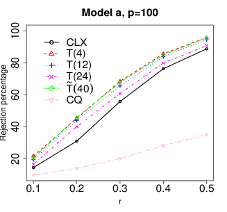
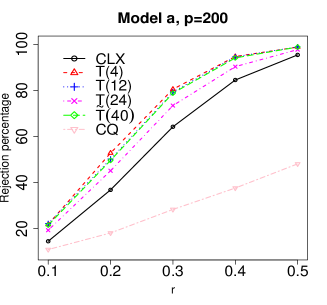
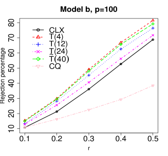
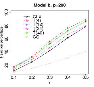
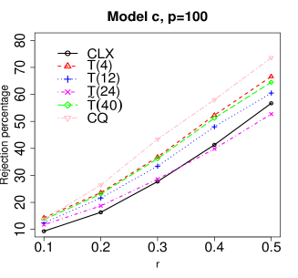
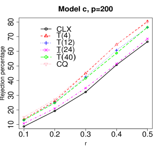
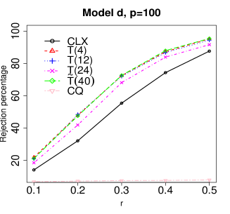
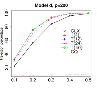
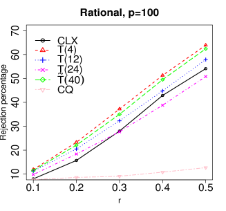
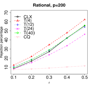
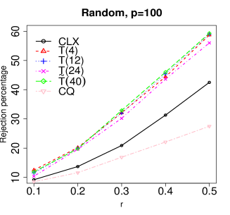
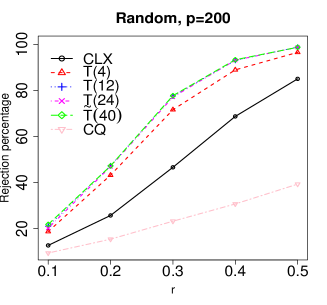
where $\widehat{\Sigma}$ is the pooled sample covariance matrix and the minimization is taken over a prespecified finite set $\Lambda_{n}$. Moreover, we employ the data dependent method in Section 3.2 to select $k$ with the upper bound $M^{\prime}=40$ (we also tried $M^{\prime}=20,80$ and found that the results are basically the same as those with $M^{\prime}=40$). For the purpose of comparison, we also implemented the Hotelling’s $T^{2}$ test and the two sample tests proposed in Bai and Saranadasa (1996), Chen and Qin (2010), and Cai et al. (2014). As the results under the Gamma model are qualitatively similar to those under the Gaussian model, we only present the results from the Gaussian model. Table 1 summarizes the sizes and powers in cases 1 and 2. The empirical powers in case 3 with $r$ ranging from 0.1 to 0.5 are presented in Figure 3. Some remarks are in order regarding the simulation results: (i) the empirical sizes are reasonably close to the nominal level 5% for all the tests; (ii) the proposed tests and the maximum type test in Cai et al. (2014) significantly outperform the sum-of-squares type testing procedures in terms of power under Models (a), (b) and (d); Under Model (c), the proposed method is quite competitive to Chen and Qin (2010)’s test which delivers more power than Cai et al. (2014)’s test in some cases; (iii) $T_{fe,n}(k)$ is consistently more powerful than Cai et al. (2014)’s test in almost all the cases; (iv) the modified test $\widetilde{T}_{fe,n}(M^{\prime})$ is insensitive to the upper bound $M^{\prime}$ (as shown in our unreported results). And its power is very competitive to $T_{fe,n}(k)$ with a suitably chosen $k$.

4.2 Power comparison under different signal allocations

We conduct additional simulations to compare the power of the proposed method with alternative approaches under different signal allocations. The data are generated from (15) with Gaussian distribution and bandable covariance structure (b). Let $k=\lfloor 0.1p\rfloor$ and consider the following four patterns of allocation, where the locations of the nonzero entries are drawn without replacement from $\{1,2,\dots,p\}$.

• (Square root): the nonzero entries are equal $\sqrt{4r\log(p)/n}\sqrt{j/k}$ for $1\leq j\leq k$.

• (Linear): the nonzero entries are equal $\sqrt{4r\log(p)/n}(j/k)$ for $1\leq j\leq k$.

• (Rational): the nonzero entries are equal $\sqrt{4r\log(p)/n}(1/j)$ for $1\leq j\leq k$.

• (Random): the nonzero entries are drawn uniformly from $(-\sqrt{4r\log(p)/n},\sqrt{4r\log(p)/n})$.

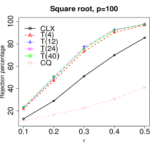
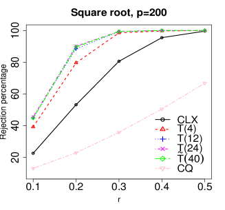
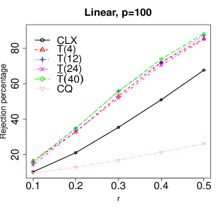
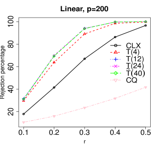
Figure 4 reports the empirical rejection probabilities for $p=100,200$, and $r$ ranging from 0.1 to 0.5. We observe that the slower the strength of the signals decays, the higher power the tests can generate. The proposed method generally outperforms the two sample tests in Chen and Qin (2010) and Cai et al. (2014) especially when the magnitudes of signals decay slowly. This result makes intuitive sense as when the magnitudes of signals are close, the top few signals together provide a stronger indication for the violation from the null as compared to the indication using only the largest signal. To sum up, the numerical results demonstrate the advantages of the proposed method over some competitors in the literature.

5 Concluding remark

In this paper, we developed a new class of tests named maximum sum-of-squares tests for conducting inference on high dimensional mean under sparsity assumption. The maximum type test has been shown to be optimal under very strong sparsity [Arias-Castro et al. (2011)]. Our result suggests that even for very sparse signal (e.g. $k$ grows slowly with $n$), the maximum type test may be improved. It is worth mentioning that our method can be extended to more general settings. For example, consider a parametric model with the negative log-likelihood (or more generally loss function) $\mathcal{L}(Y,X^{\prime}\beta)$, where $\beta\in\mathbb{R}^{p}$ is the parameter of interest, $X$ is the $p$-dimensional covariate and $Y$ is the response variable. We are interested in testing $H_{0}:\beta=0_{p\times 1}$ versus $H_{a,k}:\beta\in\Theta_{a,k}.$ Given $n$ observations $\{Y_{i},X_{i}\}^{n}_{i=1}$, the LR test for testing $H_{0}$ against $H_{a,k}$ is then defined as $LR_{n}(\beta)=2\sum^{n}_{i=1}\mathcal{L}(Y_{i},0)-2\min_{\beta\in\Theta_{a,k}}\sum^{n}_{i=1}\mathcal{L}(Y_{i},X_{i}^{\prime}\beta).$ In the case of linear model, it is related with the maximum spurious correlations recently considered in Fan et al. (2015) under the null. It is of interest to study the asymptotic properties of $LR_{n}(\beta)$ and investigate the Wilks phenomenon in this more general context.

6 Technical appendix

6.1 Preliminaries

We provide proofs of the main results in the paper. Throughout the appendix, let $C$ be a generic constant which is different from line to line. Define the unit sphere $\mathbb{S}^{p-1}=\{b\in\mathbb{R}^{p}:|b|=1\}$.

For any $1\leq k\leq p$, define

$$\mathcal{A}(t;k)=\underset{j=1}{\overset{\binom{p}{k}}{\bigcap}}\mathcal{A}_{j}(t),\quad\mathcal{A}_{j}(t)=\{w\in\mathbb{R}^{p}:w_{S_{j}}^{\prime}w_{S_{j}}\leq t\}.$$

Here $S_{j}$ is the $j$th subset of $[p]:=\{1,2,\dots,p\}$ with cardinality $k$ for $1\leq j\leq\binom{p}{k}$. It is straightforward to verify that $\mathcal{A}_{j}(t)$ is convex and it only depends on $w_{S_{j}}$, i.e. the components in $S_{j}$. The dual representation [see Rockafellar (1970)] for the convex set $\mathcal{A}_{j}(t)$ with $1\leq j\leq\binom{p}{k}$ is given by

$$\mathcal{A}_{j}(t)=\bigcap_{v\in\mathbb{S}^{p-1},v_{S_{j}}\in\mathbb{S}^{k-1}}\{w\in\mathbb{R}^{p}:w^{\prime}v\leq\sqrt{t}\},$$

where we have used the fact that $\sup_{v\in\mathbb{S}^{p-1},v_{S_{j}}\in\mathbb{S}^{k-1}}w^{\prime}v=|w_{S_{j}}|$ by the Cauchy-Schwartz inequality. Define $\mathcal{F}=\{v\in\mathbb{S}^{p-1},||v||_{0}\leq k\}$. It is not hard to see that

$$\mathcal{A}(t;k)=\bigcap_{v\in\mathcal{F}}\{w\in\mathbb{R}^{p}:w^{\prime}v\leq\sqrt{t}\}.$$

Let $\mathcal{X}$ be a subset of a Euclidean space and let $\epsilon>0$. A subset $N_{\epsilon}$ of $\mathcal{X}$ is called an $\epsilon$-net of $\mathcal{X}$ if every point $x\in\mathcal{X}$ can be approximated to within $\epsilon$ by some point $y\in N_{\epsilon}$, i.e. $|x-y|\leq\epsilon$. The minimal cardinality of an $\epsilon$-net of $\mathcal{X}$, if finite, is denoted by $N(\mathcal{X},\epsilon)$ and is called the covering number of $\mathcal{X}$.

Lemma 6.1.

For $\epsilon>0$, there exists an $\epsilon$-net of $\mathcal{F}$, denoted by $\mathcal{F}_{\epsilon}$, such that $||\mathcal{F}_{\epsilon}||_{0}\leq\left\{\frac{(2+\epsilon)ep}{\epsilon k}\right\}^{k}$ and

$$\bigcap_{v\in\mathcal{F}_{\epsilon}}\{w\in\mathbb{R}^{p}:w^{\prime}v\leq(1-\epsilon)\sqrt{t}\}\subseteq\mathcal{A}(t;k)\subseteq\bigcap_{v\in\mathcal{F}_{\epsilon}}\{w\in\mathbb{R}^{p}:w^{\prime}v\leq\sqrt{t}\}.$$ (16)

Proof of Lemma 6.1.

For the unit sphere $\mathbb{S}^{k-1}$ equipped with the Euclidean metric, it is well-known that the $\epsilon$-covering number $N(\mathbb{S}^{k-1},\epsilon)\leq(1+2/\epsilon)^{k}$, see e.g. Lemma 5.2 of Vershynin (2012). Notice that

$$\mathcal{F}=\{v\in\mathbb{S}^{p-1},||v||_{0}\leq k\}=\bigcup_{S\subseteq[p]:||S||_{0}=k}\{v\in\mathbb{S}^{p-1}:v_{S}\in\mathbb{S}^{k-1}\},$$

where $[p]=\{1,2,\dots,p\}$. Because $\binom{p}{k}\leq(ep/k)^{k}$, we have

$$N(\mathcal{F},\epsilon)\leq\binom{p}{k}\left(1+\frac{2}{\epsilon}\right)^{k}\leq\left\{\frac{(2+\epsilon)ep}{\epsilon k}\right\}^{k}.$$

Recall that

$$\mathcal{A}(t;k)=\bigcap_{v\in\mathcal{F}}\{w\in\mathbb{R}^{p}:w^{\prime}v\leq\sqrt{t}\}.$$

Let $\mathcal{F}_{\epsilon}$ be an $\epsilon$-net of $\mathcal{F}$ with cardinality $N(\mathcal{F},\epsilon)$, and $A_{1}(t):=A_{1}(t;\epsilon)=\bigcap_{v\in\mathcal{F}_{\epsilon}}\{w\in\mathbb{R}^{p}:w^{\prime}v\leq(1-\epsilon)\sqrt{t}\}$. It is easy to see that

$$\mathcal{A}(t;k)\subseteq\bigcap_{v\in\mathcal{F}_{\epsilon}}\{w\in\mathbb{R}^{p}:w^{\prime}v\leq\sqrt{t}\}.$$

For any $v\in\mathcal{F}$, we can find $v_{0}\in\mathcal{F}_{\epsilon}$ such that $|v-v_{0}|\leq\epsilon.$ Thus for $w\in A_{1}(t)$, we have

$$w^{\prime}v=w^{\prime}v_{0}+|v-v_{0}|\frac{w^{\prime}(v-v_{0})}{|v-v_{0}|}\leq(1-\epsilon)\sqrt{t}+\epsilon\max_{v_{1}\in\mathcal{F}}w^{\prime}v_{1}.$$

Taking maximum over $v\in\mathcal{F}$, we obtain $\max_{v\in\mathcal{F}}w^{\prime}v\leq(1-\epsilon)\sqrt{t}+\epsilon\max_{v_{1}\in\mathcal{F}}w^{\prime}v_{1}$, which implies that $\max_{v\in\mathcal{F}}w^{\prime}v\leq\sqrt{t}$ and thus $w\in\mathcal{A}(t;k).$ $\diamondsuit$

6.2 Proofs of the main results

Proof of Theorem 2.1.

The triangle inequality yields that

$$\sup_{t\geq 0}\left|P\left(T_{fe,n}^{*}(k)\leq t\bigg{|}X_{1}^{n}\right)-P\left(T_{fe,n}(k)\leq t\right)\right|$$

$$\leq \sup_{t\geq 0}\left|P\left(T_{n}(k)\leq t\right)-P\left(T_{fe,n}(k)\leq t\right)\right|$$

$$+\sup_{t\geq 0}\left|P\left(T_{n}(k)\leq t\right)-P\left(T_{fe,n}^{*}(k)\leq t\bigg{|}X_{1}^{n}\right)\right|:=\rho_{1,n}+\rho_{2,n}.$$

We bound $\rho_{1,n}$ and $\rho_{2,n}$ in Step 1 and Step 2 respectively.

Step 1 (bounding $\rho_{1,n}$): Let $\widehat{\xi}_{j}=\frac{|\widehat{z}_{j}|}{\sqrt{\widehat{\gamma}_{jj}}}$ and $\widehat{\xi}_{(j)}$ be the order statistic such that

$$\widehat{\xi}_{(1)}\geq\widehat{\xi}_{(2)}\geq\cdots\geq\widehat{\xi}_{(p)}.$$

Similarly we can define $\xi_{j}$ and $\xi_{(j)}$ in the same way as $\widehat{\xi}_{j}$ and $\widehat{\xi}_{(j)}$ by replacing $\widehat{\Gamma}$ with the precision matrix $\Gamma$. We have

$$|\widehat{\xi}_{j}-\xi_{j}|\leq\left|\frac{|\widehat{z}_{j}|}{\sqrt{\widehat{\gamma}_{jj}}}-\frac{|z_{j}|}{\sqrt{\widehat{\gamma}_{jj}}}\right|+\left|\frac{|z_{j}|}{\sqrt{\widehat{\gamma}_{jj}}}-\frac{|z_{j}|}{\sqrt{\gamma_{jj}}}\right|\leq\frac{|z_{j}-\widehat{z}_{j}|}{\sqrt{\widehat{\gamma}_{jj}}}+\left|\frac{\sqrt{\gamma_{jj}}-\sqrt{\widehat{\gamma}_{jj}}}{\sqrt{\gamma_{jj}}\sqrt{\widehat{\gamma}_{jj}}}\right||z_{j}|:=I_{1}+I_{2}.$$

By Proposition 2.1, we have $\max_{1\leq j\leq p}|\widehat{\Gamma}_{j}-\Gamma_{j}|_{1}=O_{p}(d\sqrt{\log(p)/n})$ and $\sup_{1\leq j\leq p}|\gamma_{jj}-\widehat{\gamma}_{jj}|=O_{p}(\sqrt{d\log(p)/n})$. Also note that $c_{1}<\min_{1\leq j\leq p}\gamma_{jj}\leq\max_{1\leq j\leq p}\gamma_{jj}<c_{2}$ for some constants $0<c_{1}\leq c_{2}<\infty.$ Together with the fact that $|\bar{X}|_{\infty}=O_{p}(\sqrt{\log(p)/n})$, we deduce

$$\sup_{1\leq j\leq p}|z_{j}-\widehat{z}_{j}|\leq\max_{1\leq j\leq p}|\widehat{\Gamma}_{j}-\Gamma_{j}|_{1}|\bar{X}|_{\infty}=O_{p}\left(d\log(p)/n\right),$$

and

$$\sup_{1\leq j\leq p}|\sqrt{\gamma_{jj}}-\sqrt{\widehat{\gamma}_{jj}}|=\sup_{1\leq j\leq p}\left|\frac{\gamma_{jj}-\widehat{\gamma}_{jj}}{\sqrt{\gamma_{jj}}+\sqrt{\widehat{\gamma}_{jj}}}\right|=O_{p}\left(\sqrt{d\log(p)/n}\right).$$ (17)

As $\sup_{1\leq j\leq p}|z_{j}|=O_{p}(\sqrt{\log(p)/n})$, we obtain

$$\sup_{1\leq j\leq p}|\widehat{\xi}_{j}-\xi_{j}|=O_{p}\left(d\log(p)/n\right),$$

and

$$\sup_{1\leq j\leq p}|\widehat{\xi}_{j}^{2}-\xi_{j}^{2}|=O_{p}\left(d\log(p)/n\right)\sup_{1\leq j\leq p}|\widehat{\xi}_{j}+\xi_{j}|=O_{p}\left(d(\log(p)/n)^{3/2}\right).$$

Thus we deduce that

$$\left|T_{n}(k)-T_{fe,n}(k)\right|\leq \max_{1\leq j_{1}<j_{2}<\cdots<j_{k}\leq p}n\sum^{k}_{l=1}\left|\xi_{j_{l}}^{2}-\widehat{\xi}_{j_{l}}^{2}\right|$$

$$\leq nk\max_{1\leq j\leq p}|\widehat{\xi}_{j}^{2}-\xi_{j}^{2}|=O_{p}\left(kd(\log(p))^{3/2}/\sqrt{n}\right).$$

By the assumption $k^{2}d(\log(np))^{5/2}/\sqrt{n}=o(1)$, we can pick $\zeta_{1}$ and $\zeta_{2}$ such that

$$P(\left|T_{n}(k)-T_{fe,n}(k)\right|\geq\zeta_{1})\leq\zeta_{2},$$

where $\zeta_{1}k\log(np)=o(1)$ and $\zeta_{2}=o(1)$. Define the event $\mathcal{B}=\{\left|T_{n}(k)-T_{fe,n}(k)\right|<\zeta_{1}\}$. Then we have

$$|P(T_{n}(k)\leq t)-P(T_{fe,n}(k)\leq t)|$$

$$\leq P(T_{n}(k)\leq t,T_{fe,n}(k)>t)+P(T_{n}(k)>t,T_{fe,n}(k)\leq t)$$

$$\leq P(T_{n}(k)\leq t,T_{fe,n}(k)>t,\mathcal{B})+P(T_{n}(k)>t,T_{fe,n}(k)\leq t,\mathcal{B})+2\zeta_{2}$$

$$\leq P(t-\zeta_{1}<T_{n}(k)\leq t)+P(t+\zeta_{1}\geq T_{n}(k)>t)+2\zeta_{2}.$$

Let $V_{i}=\text{diag}^{-1/2}(\Gamma)\Gamma X_{i}$ and $V=\sum^{n}_{i=1}V_{i}/\sqrt{n}$. Notice that $\left\{T_{n}(k)\leq t\right\}=\left\{V\in\mathcal{A}(t;k)\right\}=\{\max_{v\in\mathcal{F}}v^{\prime}V\leq\sqrt{t}\}.$ By Lemma 6.1, we can find an $\epsilon$-net $\mathcal{F}_{\epsilon}$ of $\mathcal{F}$ such that $||\mathcal{F}_{\epsilon}||_{0}\leq\{(2+\epsilon)ep/(\epsilon k)\}^{k}$ and

$$A_{1}(t):=\bigcap_{v\in\mathcal{F}_{\epsilon}}\{v^{\prime}V\leq(1-\epsilon)\sqrt{t}\}\subseteq\mathcal{A}(t;k)\subseteq A_{2}(t):=\bigcap_{v\in\mathcal{F}_{\epsilon}}\{v^{\prime}V\leq\sqrt{t}\}.$$

We set $\epsilon=1/n$ throughout the following arguments. Notice that

$$P(t-\zeta_{1}<T_{n}(k)\leq t)$$

$$= P(T_{n}(k)\leq t)-P(T_{n}(k)\leq t-\zeta_{1})$$

$$\leq P(\max_{v\in\mathcal{F}_{\epsilon}}v^{\prime}V\leq\sqrt{t})-P(\max_{v\in\mathcal{F}_{\epsilon}}v^{\prime}V\leq(1-\epsilon)\sqrt{t-\zeta_{1}})$$

$$\leq P((1-\epsilon)(\sqrt{t}-\sqrt{\zeta_{1}})\leq\max_{v\in\mathcal{F}_{\epsilon}}v^{\prime}V\leq\sqrt{t})$$

$$\leq P((1-\epsilon)(\sqrt{t}-\sqrt{\zeta_{1}})\leq\max_{v\in\mathcal{F}_{\epsilon}}v^{\prime}V\leq(1-\epsilon)\sqrt{t})+P((1-\epsilon)\sqrt{t}<\max_{v\in\mathcal{F}_{\epsilon}}v^{\prime}V\leq\sqrt{t})$$

$$:= I_{1}+I_{2}.$$

Because $\phi(\Gamma;k)>c>0$, we have ${\mbox{var}}(\sum^{n}_{i=1}v^{\prime}V_{i}/\sqrt{n})>c^{\prime}$ for all $v\in\mathcal{F}$ and some constant $c^{\prime}>0.$ By the Nazarov inequality [see Lemma A.1 in Chernozhukov et al. (2015) and Nazarov (2003)], we have

$$I_{1}\leq C\sqrt{\zeta_{1}k\log(np/k)}=o(1).$$ (18)

To deal with $I_{2}$, we note when $t\leq k^{3}\{\log(np/k)\}^{2}$, $\epsilon\sqrt{t}\leq k^{3/2}\log(np/k)/n$. Again by the Nazarov’s inequality, we have

$$I_{2}\leq P(\sqrt{t}-k^{3/2}\log(np/k)/n<\max_{v\in\mathcal{F}_{\epsilon}}v^{\prime}V\leq\sqrt{t})\leq k^{2}\log(np/k)\sqrt{\log(np/k)}/n=o(1).$$

When $t>k^{3}\{\log(np/k)\}^{2}$, we have

$$I_{2}\leq P((1-\epsilon)\sqrt{t}\leq\max_{v\in\mathcal{F}_{\epsilon}}v^{\prime}V)\leq\frac{\mathbb{E}\max_{v\in\mathcal{F}_{\epsilon}}v^{\prime}V}{(1-\epsilon)k^{3/2}\log(np/k)}.$$

By Lemma 7.4 in Fan et al. (2015), we have $\mathbb{E}\max_{v\in\mathcal{F}_{\epsilon}}v^{\prime}V\leq C\sqrt{k\log(np/k)}.$ It thus implies that

$$I_{2}\leq\frac{C\sqrt{k\log(np/k)}}{(1-\epsilon)k^{3/2}\log(np/k)}=o(1).$$

Summarizing the above derivations, we have $\rho_{1,n}=o(1)$.

Step 2 (bounding $\rho_{2,n}$): Define $\widehat{V}^{*}=\text{diag}^{-1/2}(\widehat{\Gamma})\widehat{\Gamma}\sum^{n}_{i=1}(X_{i}-\bar{X})e_{i}/\sqrt{n}$ with $e_{i}\sim^{i.i.d}N(0,1)$, where $e_{i}$’s are independent of $X^{n}_{1}.$ Further define

$$\bar{\rho}=\max\{|P(V\in A_{1}(t))-P(\widehat{V}^{*}\in A_{1}(t)|X^{n}_{1})|,|P(V\in A_{2}(t))-P(\widehat{V}^{*}\in A_{2}(t)|X^{n}_{1})|\}.$$

Using similar arguments in Step 1, we have

$$P(\widehat{V}^{*}\in\mathcal{A}(t;k)|X^{n}_{1})\leq P(\widehat{V}^{*}\in A_{2}(t)|X^{n}_{1})\leq P(V\in A_{2}(t))+\bar{\rho}$$

$$\leq P(V\in A_{1}(t))+\bar{\rho}+o(1)$$

$$\leq P(V\in\mathcal{A}(t;k))+\bar{\rho}+o(1).$$

Similarly we have $P(\widehat{V}^{*}\in\mathcal{A}(t;k)|X^{n}_{1})\geq P(V\in\mathcal{A}(t;k))-\bar{\rho}-o(1)$. Together, we obtain

$$|P(\widehat{V}^{*}\in\mathcal{A}(t;k)|X^{n}_{1})-P(V\in\mathcal{A}(t;k))|\leq\bar{\rho}+o(1).$$

Let $D=\text{diag}^{-1/2}(\Gamma)\Gamma\text{diag}^{-1/2}(\Gamma)$ and $\widehat{D}=\text{diag}^{-1/2}(\widehat{\Gamma})\widehat{\Gamma}\widehat{\Sigma}\widehat{\Gamma}^{\prime}\text{diag}^{-1/2}(\widehat{\Gamma}),$ where $\widehat{\Sigma}=\sum^{n}_{i=1}(X_{i}-\bar{X})(X_{i}-\bar{X})^{\prime}/n$. Define $\Delta_{n}=\max_{u,v\in\mathcal{F}}|u(\widehat{D}-D)v|.$ Notice that $V\sim N(0,D)$ and $\widehat{V}^{*}|X^{n}_{1}\sim N(0,\widehat{D})$. To bound $\bar{\rho}$, we note that by equation (49) in Chernozhukov et al. (2015),

$$\sup_{t\geq 0}|P(V\in A_{1}(t))-P(\widehat{V}^{*}\in A_{1}(t)|X^{n}_{1})|$$

$$= \sup_{t\geq 0}|P(\max_{v\in\mathcal{F}_{\epsilon}}u^{\prime}V\leq\sqrt{t})-P(\max_{u\in\mathcal{F}_{\epsilon}}u^{\prime}\widehat{V}^{*}\leq\sqrt{t}|X^{n}_{1})|$$

$$\leq C\Delta_{n}^{1/3}(k\log(np/k))^{2/3}.$$

and similarly $|P(V\in A_{2}(t))-P(\widehat{V}^{*}\in A_{2}(t)|X^{n}_{1})|\leq C\Delta_{n}^{1/3}(k\log(np/k))^{2/3}.$ Therefore we get

$$\rho_{2,n}\leq C\Delta_{n}^{1/3}(\log(p))^{2/3}+o(1).$$

Step 3: Finally we bound $\Delta_{n}$. Note that for any $u,v\in\mathcal{F}$,

$$|u^{\prime}(\widehat{D}-D)v|$$

$$\leq |u^{\prime}(\widehat{D}-\text{diag}^{-1/2}(\widehat{\Gamma})\widehat{\Gamma}^{\prime}\text{diag}^{-1/2}(\widehat{\Gamma}))v|+|u^{\prime}(\text{diag}^{-1/2}(\widehat{\Gamma})\widehat{\Gamma}^{\prime}\text{diag}^{-1/2}(\widehat{\Gamma})-\text{diag}^{-1/2}(\widehat{\Gamma})\Gamma\text{diag}^{-1/2}(\widehat{\Gamma}))v|$$

$$+|u^{\prime}(\text{diag}^{-1/2}(\widehat{\Gamma})\Gamma\text{diag}^{-1/2}(\widehat{\Gamma})-D)v|:=J_{1}+J_{2}+J_{3}.$$

For the first term, we have

$$J_{1}= |u^{\prime}\text{diag}^{-1/2}(\widehat{\Gamma})(\widehat{\Gamma}\widehat{\Sigma}^{\prime}\widehat{\Gamma}-\widehat{\Gamma}^{\prime})\text{diag}^{-1/2}(\widehat{\Gamma})v|$$

$$\leq |\text{diag}^{-1/2}(\widehat{\Gamma})u|_{1}|(\widehat{\Gamma}\widehat{\Sigma}^{\prime}\widehat{\Gamma}-\widehat{\Gamma}^{\prime})\text{diag}^{-1/2}(\widehat{\Gamma})v|_{\infty}$$

$$\leq |\text{diag}^{-1/2}(\widehat{\Gamma})u|_{1}|\text{diag}^{-1/2}(\widehat{\Gamma})v|_{1}||\widehat{\Gamma}\widehat{\Sigma}\widehat{\Gamma}^{\prime}-\widehat{\Gamma}^{\prime}||_{\infty}$$

$$\leq k|\text{diag}^{-1/2}(\widehat{\Gamma})u|_{2}|\text{diag}^{-1/2}(\widehat{\Gamma})v|_{2}||\widehat{\Gamma}\widehat{\Sigma}\widehat{\Gamma}^{\prime}-\widehat{\Gamma}^{\prime}||_{\infty}=O_{p}(k\sqrt{d\log(p)/n}),$$

where we have used Proposition 2.1. To handle the second term, note that

$$J_{2}= |v^{\prime}\text{diag}^{-1/2}(\widehat{\Gamma})(\widehat{\Gamma}-\Gamma)\text{diag}^{-1/2}(\widehat{\Gamma})u|$$

$$\leq |\text{diag}^{-1/2}(\widehat{\Gamma})v|_{1}|(\widehat{\Gamma}-\Gamma)\text{diag}^{-1/2}(\widehat{\Gamma})u|_{\infty}$$

$$\leq \sqrt{k}|\text{diag}^{-1/2}(\widehat{\Gamma})v|_{2}|\text{diag}^{-1/2}(\widehat{\Gamma})u|_{\infty}\max_{1\leq j\leq p}|\widehat{\Gamma}_{j}-\Gamma_{j}|_{1}=O_{p}(d\sqrt{k\log(p)/n}).$$

Finally, we have

$$J_{3}\leq |u^{\prime}(\text{diag}^{-1/2}(\widehat{\Gamma})\Gamma\text{diag}^{-1/2}(\widehat{\Gamma})-\text{diag}^{-1/2}(\Gamma)\Gamma\text{diag}^{-1/2}(\widehat{\Gamma}))v|+|u^{\prime}(\text{diag}^{-1/2}(\Gamma)\Gamma\text{diag}^{-1/2}(\widehat{\Gamma})-D)v|$$

$$\leq ||\Gamma||_{2}||\text{diag}^{-1/2}(\widehat{\Gamma})||_{2}\max_{1\leq j\leq p}|1/\sqrt{\gamma_{jj}}-1/\sqrt{\widehat{\gamma}_{jj}}|+||\Gamma||_{2}||\text{diag}^{-1/2}(\Gamma)||_{2}\max_{1\leq j\leq p}|1/\sqrt{\gamma_{jj}}-1/\sqrt{\widehat{\gamma}_{jj}}|$$

$$= \sqrt{d\log(p)/n}.$$

Under the assumption that $k^{2}d(\log(np))^{5/2}/\sqrt{n}=o(1)$, we have $(\log(np))^{2}J_{i}=o_{p}(1)$ for $1\leq i\leq 3$. Therefore we get $(\log(np))^{2}\Delta_{n}=o_{p}(1)$, which implies that $\rho_{2,n}=o_{p}(1)$. The proof is thus completed by combining Steps 1-3. $\diamondsuit$

Proof of Theorem 2.2.

We first note that by the triangle inequality,

$$\sup_{t_{M}\geq t_{M-1}\geq\cdots\geq t_{1}\geq 0}\left|P\left(\bigcap^{M}_{j=1}\{T_{fe,n}^{*}(j)\leq t_{j}\}\bigg{|}X_{1}^{n}\right)-P\left(\bigcap^{M}_{j=1}\{T_{fe,n}(j)\leq t_{j}\}\right)\right|$$

$$\leq \sup_{t_{M}\geq t_{M-1}\geq\cdots\geq t_{1}\geq 0}\left|P\left(\bigcap^{M}_{j=1}\{T_{n}(j)\leq t_{j}\}\right)-P\left(\bigcap^{M}_{j=1}\{T_{fe,n}(j)\leq t_{j}\}\right)\right|$$

$$+\sup_{t_{M}\geq t_{M-1}\geq\cdots\geq t_{1}\geq 0}\left|P\left(\bigcap^{M}_{j=1}\{T_{n}(j)\leq t_{j}\}\right)-P\left(\bigcap^{M}_{j=1}\{T_{fe,n}^{*}(j)\leq t_{j}\}\bigg{|}X_{1}^{n}\right)\right|:=\varrho_{1,n}+\varrho_{2,n}.$$

Step 1 (bounding $\varrho_{1,n}$): Following the proof of Theorem 2.1, we have for any $1\leq j\leq M$,

$$\max_{1\leq j\leq M}\left|T_{n}(j)-T_{fe,n}(j)\right|\leq nM\max_{1\leq j\leq p}|\widehat{\xi}_{j}^{2}-\xi_{j}^{2}|=O_{p}\left(Md(\log(p))^{3/2}/\sqrt{n}\right).$$

Under the assumption that $M^{4}d(\log(np))^{5/2}/\sqrt{n}=o(1)$, one can pick $\zeta$ such that $P(\max_{1\leq j\leq M}\left|T_{n}(j)-T_{fe,n}(j)\right|>\zeta)=o(1)$ and $\zeta M^{3}\log(np)=o(1)$. Define $\mathcal{B}=\{\max_{1\leq j\leq M}\left|T_{n}(j)-T_{fe,n}(j)\right|\leq\zeta\}$. We note that

$$\left|P\left(\bigcap^{M}_{j=1}\{T_{n}(j)\leq t_{j}\}\right)-P\left(\bigcap^{M}_{j=1}\{T_{fe,n}(j)\leq t_{j}\}\right)\right|$$

$$\leq P\left(\bigcap^{M}_{j=1}\{T_{n}(j)\leq t_{j}\},\bigcup^{M}_{j=1}\{T_{fe,n}(j)>t_{j}\},\mathcal{B}\right)$$

$$+P\left(\bigcup^{M}_{j=1}\{T_{n}(j)>t_{j}\},\bigcap^{M}_{j=1}\{T_{fe,n}(j)\leq t_{j}\},\mathcal{B}\right)+o(1)$$

$$\leq P\left(\bigcup^{M}_{j=1}\{t_{j}-\zeta<T_{n}(j)\leq t_{j}\}\right)+P\left(\bigcup^{M}_{j=1}\{t_{j}<T_{n}(j)\leq t_{j}+\zeta\}\right)+o(1).$$

By the arguments in the proof of Theorem 2.1, we have $P\left(t_{j}-\zeta<T_{n}(j)\leq t_{j}\right)=o(1)$. A careful inspection of the proof shows that

$$\max_{1\leq j\leq M}\max\{P\left(t_{j}-\zeta<T_{n}(j)\leq t_{j}\right),P\left(t_{j}<T_{n}(j)\leq t_{j}+\zeta\right)\}$$

$$\leq C\left\{\sqrt{\zeta M\log(np)}+M^{2}(\log(np))^{3/2}/n+1/(M\sqrt{\log(np/M)})\right\},$$

where the uniformity over $1\leq j\leq M$ is due to the fact that the constant $C$ in (18) is independent of $t$. By the union bound, we deduce that

$$\left|P\left(\bigcap^{M}_{j=1}\{T_{n}(j)\leq t_{j}\}\right)-P\left(\bigcap^{M}_{j=1}\{T_{fe,n}(j)\leq t_{j}\}\right)\right|$$

$$\leq \sum^{M}_{j=1}\left(P\left(t_{j}-\zeta<T_{n}(j)\leq t_{j}\right)+P\left(t_{j}<T_{n}(j)\leq t_{j}+\zeta\right)\right)+o(1)$$

$$\leq M\max_{1\leq j\leq M}\left(P\left(t_{j}-\zeta<T_{n}(j)\leq t_{j}\right)+P\left(t_{j}<T_{n}(j)\leq t_{j}+\zeta\right)\right)+o(1)$$

$$\leq C\left(\sqrt{\zeta M^{3}\log(np)}+M^{3}(\log(np))^{3/2}/n+1/\sqrt{\log(np/M)}\right)+o(1)=o(1).$$

Step 2 (bounding $\varrho_{2,n}$): For $\mathbf{t}=(t_{1},\dots,t_{M})$, define

$$\mathcal{A}(\mathbf{t})=\bigcap^{M}_{j=1}\mathcal{A}(t_{j};j)=\bigcap^{M}_{j=1}\bigcap_{S\subseteq[p],||S||_{0}=j}\{w\in\mathbb{R}^{p}:w_{S}^{\prime}w_{S}\leq t_{j}\}.$$

It is easy to see that

$$\bigcap^{M}_{j=1}\{T_{n}(j)\leq t_{j}\}=\{V\in\mathcal{A}(\mathbf{t})\},\quad\bigcap^{M}_{j=1}\{T_{fe,n}^{*}(j)\leq t_{j}\}=\{\widehat{V}^{*}\in\mathcal{A}(\mathbf{t})\}.$$

By Lemma 6.1, we know for any fixed $\mathbf{t}$,

$$\mathbf{A}_{1}(\mathbf{t}):=\bigcap_{j=1}^{M}A_{1}(t_{j})\subseteq\mathcal{A}(\mathbf{t})\subseteq\mathbf{A}_{2}(\mathbf{t}):=\bigcap_{j=1}^{M}A_{2}(t_{j}),$$

where $A_{1}(t_{j})=\bigcap_{v\in\mathcal{F}_{\epsilon}(j)}\{w\in\mathbb{R}^{p}:w^{\prime}v\leq(1-\epsilon)\sqrt{t_{j}}\}$ and $A_{2}(t_{j})=\bigcap_{v\in\mathcal{F}_{\epsilon}(j)}\{w\in\mathbb{R}^{p}:w^{\prime}v\leq\sqrt{t_{j}}\}$ with $\epsilon=1/n$ and $\mathcal{F}_{\epsilon}(j)$ being an $\epsilon$-net for $\mathcal{F}(j):=\{v\in\mathbb{S}^{p-1}:||v||_{0}\leq j\}$. Note that $\mathbf{A}_{1}(\mathbf{t})$ and $\mathbf{A}_{2}(\mathbf{t})$ are both intersections of no more than $M\{(2+1/n)epn\}^{M}$ half spaces. Thus following the arguments in Steps 2 and 3 of the proof of Theorem 2.1, we can show that $\varrho_{2,n}=o_{p}(1)$, which completes our proof. $\diamondsuit$

Proof of Theorem 2.3.

The proof contains two steps. In the first step, we establish the consistency of the infeasible test $T_{n}(k)$, while in the second step we further show that the estimation effect caused by replacing $\Gamma$ with $\widehat{\Gamma}$ is asymptotically negligible.
Step 1: Consider the infeasible test $T_{n}(k)=\max_{1\leq j_{1}<j_{2}<\cdots<j_{k}\leq n}\sum^{k}_{l=1}\frac{nz_{j_{l}}^{2}}{\gamma_{j_{l},j_{l}}}.$ Define $\widetilde{\theta}=(\widetilde{\theta}_{1},\dots,\widetilde{\theta}_{p})^{\prime}$ with $\widetilde{\theta}_{j}=(\Gamma\theta)_{j}/\sqrt{\gamma_{jj}}$, and $q_{j}=\frac{z_{j}-(\Gamma\theta)_{j}}{\sqrt{\gamma_{jj}}}.$ Note that $\frac{z_{j}^{2}}{\gamma_{jj}}=\left(q_{j}+\widetilde{\theta}_{j}\right)^{2}.$ Also by Lemma 3 of Cai et al. (2014), we have for any $2r<a<1-2r$,

$$P\left(\max_{j\in H}|\widetilde{\theta}_{j}-\sqrt{\gamma_{jj}}\theta_{j}|=O(p^{r-a/2})\max_{j\in H}|\theta_{j}|\right)\rightarrow 1,$$ (19)

where $H$ denotes the support of $\theta$. Suppose $\sqrt{\gamma_{j_{1}^{*},j_{1}^{*}}}\theta_{j_{1}^{*}}\geq\sqrt{\gamma_{j_{2}^{*},j_{2}^{*}}}\theta_{j_{2}^{*}}\geq\cdots\geq\sqrt{\gamma_{j_{p}^{*},j_{p}^{*}}}\theta_{j_{p}^{*}}.$ We deduce that with probability tending to one,

$$T_{n}(k)= \max_{1\leq j_{1}<j_{2}<\cdots<j_{k}\leq n}\sum^{k}_{l=1}n\left(q_{j_{l}}^{2}+\widetilde{\theta}_{j_{l}}^{2}+2q_{j_{l}}\widetilde{\theta}_{j_{l}}\right)$$

$$\geq \left(n\sum^{k}_{l=1}\gamma_{j_{l}^{*},j_{l}^{*}}\theta_{j_{l}^{*}}^{2}+n\sum^{k}_{l=1}q_{j_{l}^{*}}^{2}+2n\sum^{k}_{l=1}q_{j_{l}^{*}}\sqrt{\gamma_{j_{l}^{*}j_{l}^{*}}}\theta_{j_{l}^{*}}\right)(1+o(1))$$

$$\geq \left\{n\sum^{k}_{l=1}\gamma_{j_{l}^{*},j_{l}^{*}}\theta_{j_{l}^{*}}^{2}+n\sum^{k}_{l=1}q_{j_{l}^{*}}^{2}-2n\left(\sum^{k}_{l=1}q_{j_{l}^{*}}^{2}\right)^{1/2}\left(\sum^{k}_{l=1}\gamma_{j_{l}^{*}j_{l}^{*}}\theta_{j_{l}^{*}}^{2}\right)^{1/2}\right\}(1+o(1)).$$

We claim that $n\sum^{k}_{l=1}q_{j_{l}}^{2}=O_{p}(k)$ for any $\widetilde{S}:=\{j_{1},\dots,j_{k}\}\subseteq[p].$ Note that

$${\mbox{var}}\left(\sum^{k}_{l=1}(nq_{j_{l}}^{2}-1)/\sqrt{k}\right)= \frac{2}{k}\sum^{k}_{i,l=1}\gamma_{j_{i},j_{l}}^{2}/(\gamma_{j_{i},j_{i}}\gamma_{j_{l},j_{l}})\leq\frac{C}{k}\sum^{k}_{i,l=1}\gamma_{j_{i},j_{l}}^{2}=\frac{C}{k}\text{Tr}(\Gamma_{\widetilde{S},\widetilde{S}}^{2})\leq C/\lambda_{\min}^{2}\leq C,$$

where $\text{Tr}(\cdot)$ denotes the trace of a matrix. Therefore conditional on $\widetilde{S}$, $n\sum^{k}_{l=1}q_{j_{l}}^{2}=O_{p}(k)$. As $q_{j}$ is independent of the non-zero locations of $\theta$, $n\sum^{k}_{l=1}q_{j_{l}^{*}}^{2}=O_{p}(k)$.

By the assumption that $\sum^{k}_{l=1}\gamma_{j_{l}^{*},j_{l}^{*}}\theta_{j_{l}^{*}}^{2}\geq(2k+\epsilon)\log(p)/n$ and $n\sum^{k}_{l=1}q_{j_{l}^{*}}^{2}=O_{p}(k)$, we obtain

$$T_{n}(k)\geq\left\{(2k+\epsilon)\log(p)+O_{p}(k)-O_{p}(\sqrt{(2k+\epsilon)k\log(p)})\right\}(1+o(1)).$$ (20)

Under Assumption 2.5, we have by Lemma 6 of Cai et al. (2014),

$$\max_{1\leq j_{1}<j_{2}<\cdots<j_{k}\leq p}n\sum^{k}_{l=1}q_{j_{l}}^{2}\leq kn\max_{1\leq j\leq p}q_{j}^{2}=\{2k\log(p)-k\log\log(p)\}+O_{p}(1).$$

As shown in Theorem 2.1, the bootstrap statistic $T_{fe,n}^{*}(k)$ imitates the sampling distribution of $\max_{1\leq j_{1}<j_{2}\cdots<j_{k}\leq n}\sum^{k}_{l=1}nq_{j_{l}}^{2}$. By Step 2 in the proof of Theorem 2.1, we have

$$c_{\alpha}^{*}(k)\leq\{2k\log p-k\log\log(p)\}+O_{p}(1).$$ (21)

Combining (20) and (21), we get

$$P(T_{n}(k)>c_{\alpha}^{*}(k))\rightarrow 1.$$

Step 2: Next we quantify the difference between $T_{n}(k)$ and $T_{fe,n}(k)$. Note that

$$\left|T_{n}(k)-T_{fe,n}(k)\right|\leq \max_{1\leq j_{1}<j_{2}<\cdots<j_{k}\leq p}n\sum^{k}_{l=1}\left|\xi_{j_{l}}^{2}-\widehat{\xi}_{j_{l}}^{2}\right|\leq nk\max_{1\leq j\leq p}|\widehat{\xi}_{j}^{2}-\xi_{j}^{2}|.$$

We define $\widehat{\theta}_{j}$ and $\widehat{q}_{j}$ by replacing $\Gamma$ with $\widehat{\Gamma}$ in $\widetilde{\theta}_{j}$ and $q_{j}$. Simple algebra yields that

$$\widehat{\xi}_{j}^{2}-\xi_{j}^{2}= (\widehat{q}_{j}+\widehat{\theta}_{j})^{2}-(q_{j}+\widetilde{\theta}_{j})^{2}=(\widehat{q}_{j}-q_{j}+\widehat{\theta}_{j}-\widetilde{\theta}_{j})(q_{j}+\widetilde{\theta}_{j}+\widehat{q}_{j}+\widehat{\theta}_{j}).$$ (22)

Using similar argument in Step 1 of the proof of Theorem 2.1, we obtain

$$\max_{1\leq j\leq p}|q_{j}-\widehat{q}_{j}|=O_{p}\left(d\log(p)/n\right),$$

and

$$\max_{1\leq j\leq p}|\widetilde{\theta}_{j}-\widehat{\theta}_{j}|=O_{p}(d\sqrt{\log(p)/n})\max_{1\leq j\leq p}|\theta_{j}|+O_{p}(\sqrt{d\log(p)/n})\max_{1\leq j\leq p}|\widetilde{\theta}_{j}|,$$

where we have used (9), (17), the triangle inequality and the fact that $\max_{1\leq j\leq p}|(\Gamma\theta)_{j}|\leq C\max_{1\leq j\leq p}|\widetilde{\theta}_{j}|$ for some $C>0.$ By (19), we have with probability tending to one, $\max_{j\in H}|\widetilde{\theta}_{j}|\leq(C^{\prime}+o(1))\max_{j\in H}|\theta_{j}|$ for $C^{\prime}>0.$ Define the event

$$A=\left\{\max_{1\leq j\leq p}|\theta_{j}|<C_{0}\sqrt{\log(p)/n}\right\},$$

for some large enough constant $C_{0}>0.$ On $A$, we have $\max_{1\leq j\leq p}|\widetilde{\theta}_{j}-\widehat{\theta}_{j}|=O_{p}(d\log(p)/n).$ In view of (22), we have on the event $A$,

$$|\widehat{\xi}_{j}^{2}-\xi_{j}^{2}|=O_{p}(d(\log(p)/n)^{3/2})$$

which implies that

$$\left|T_{n}(k)-T_{fe,n}(k)\right|\leq O_{p}(kd(\log(p))^{3/2}/\sqrt{n}).$$

For any $\epsilon>0$, pick $C^{\prime\prime}$ such that

$$P(\left|T_{n}(k)-T_{fe,n}(k)\right|\leq C^{{}^{\prime\prime}}kd(\log(p))^{3/2}/\sqrt{n}|A)\geq 1-\epsilon.$$

Thus we have

$$\begin{split}P(T_{fe,n}(k)>c_{\alpha}^{*}(k)|A)\geq&P(T_{n}(k)>c_{\alpha}^{*}(k)+|T_{n}(k)-T_{fe,n}(k)||A)\\ \geq&P(T_{n}(k)>c_{\alpha}^{*}(k)+C^{{}^{\prime\prime}}kd(\log(p))^{3/2}/\sqrt{n}|A)-\epsilon.\end{split}$$ (23)

Recall for $\zeta>0$ with $\zeta k\log(np)=o(1)$, we have

$$P(t\leq T_{n}(k)\leq t+\zeta)=o(1).$$

See Step 1 in the proof of Theorem 2.1. Under the assumption that $k^{2}d(\log(np))^{5/2}/\sqrt{n}=o(1)$, we have

$$P(T_{n}(k)>c_{\alpha}^{*}(k)|A)-P(T_{n}(k)>c_{\alpha}^{*}(k)+C^{{}^{\prime\prime}}kd(\log(p))^{3/2}/\sqrt{n}|A)$$

$$= P(c_{\alpha}^{*}(k)<T_{n}(k)\leq c_{\alpha}^{*}(k)+C^{{}^{\prime\prime}}kd(\log(p))^{3/2}/\sqrt{n}|A)=o(1).$$

Together with (23) and the result in Step 1, we obtain

$$P(T_{fe,n}(k)>c_{\alpha}^{*}(k)|A)\geq P(T_{n}(k)>c_{\alpha}^{*}(k)|A)-o(1)-\epsilon\rightarrow 1-\epsilon.$$

Suppose $\max_{1\leq j\leq p}|\theta_{j}|=|\theta_{k_{1}^{*}}|$. On $A^{c}$, we have for large enough $C_{0}$,

$$T_{n}(k)\geq n\left(q_{k_{1}^{*}}^{2}+\widetilde{\theta}_{k_{1}^{*}}^{2}+2q_{k_{1}^{*}}\widetilde{\theta}_{k_{1}^{*}}\right)\geq C_{1}\log(p)>2k\log(p)-k\log\log(p),$$

which holds with probability tending to one. It implies that $P(T_{n}(k)>2k\log(p)-k\log\log(p)|A^{c})\rightarrow 1.$ Similar argument indicates that

$$P(T_{fe,n}(k)>c_{\alpha}^{*}(k)|A^{c})\rightarrow 1.$$ (24)

By (23) and (24), we deduce that

$$P(T_{fe,n}(k)>c_{\alpha}^{*}(k))=P(A)P(T_{fe,n}(k)>c_{\alpha}^{*}|A)+P(A^{c})P(T_{fe,n}(k)>c_{\alpha}^{*}|A^{c})\rightarrow 1-\epsilon P(A).$$

The conclusion follows as $\epsilon$ is arbitrary.

Finally, we show the consistency of $\widetilde{T}_{fe,n}(M)$. As $\widetilde{T}_{fe,n}^{*}(M)$ imitates the sampling distribution of $\widetilde{T}_{fe,n}(M)$ under the null, we know

$$\widetilde{c}_{\alpha}^{*}(M)=\sqrt{2M}\log(p)(1+o_{p}(1)).$$

Therefore we have

$$P(\widetilde{T}_{fe,n}(M)>\widetilde{c}_{\alpha}^{*}(M))\geq P\left(\sqrt{\frac{1-M/n}{2M}}\left(T_{fe,n}(M)-M\right)>\widetilde{c}_{\alpha}^{*}(M)\right)\rightarrow 1.$$

$\diamondsuit$

Proof of Proposition 2.2.

Under Assumption 2.6, we have $|\bar{X}|_{\infty}=O_{p}(\sqrt{\log(p)/n})$ and $|Z|_{\infty}=O_{p}(\sqrt{\log(p)/n})$. By the arguments in van de Geer et al. (2014), (8), (9) and (10) still hold under the sub-gaussian assumption. Therefore using the same arguments in Step 1 of the proof of Theorem 2.1, we can pick $\zeta_{1}$ and $\zeta_{2}$ such that

$$P(\left|T_{n}(k)-T_{fe,n}(k)\right|>\zeta_{1})\leq\zeta_{2},$$

where $\zeta_{1}k\log(np)=o(1)$ and $\zeta_{2}=o(1)$. Thus we have

$$|P(T_{n}(k)\leq t)-P(T_{fe,n}(k)\leq t)|\leq P(t-\zeta_{1}<T_{n}(k)\leq t)+P(t+\zeta_{1}\geq T_{n}(k)>t)+2\zeta_{2}.$$

By Lemma 6.1, we have

$$P(t-\zeta_{1}<T_{n}(k)\leq t)$$

$$\leq P((1-\epsilon)(\sqrt{t}-\sqrt{\zeta_{1}})\leq\max_{v\in\mathcal{F}_{\epsilon}}v^{\prime}V\leq(1-\epsilon)\sqrt{t})+P((1-\epsilon)\sqrt{t}\leq\max_{v\in\mathcal{F}_{\epsilon}}v^{\prime}V\leq\sqrt{t}).$$

Corollary 2.1 in Chernozukov et al. (2015) yields that

$$P(t-\zeta_{1}<T_{n}(k)\leq t)$$

$$\leq P((1-\epsilon)(\sqrt{t}-\sqrt{\zeta_{1}})\leq\max_{v\in\mathcal{F}_{\epsilon}}v^{\prime}W\leq(1-\epsilon)\sqrt{t})+P((1-\epsilon)\sqrt{t}\leq\max_{v\in\mathcal{F}_{\epsilon}}v^{\prime}W\leq\sqrt{t})+c_{n,p,k},$$

where $\epsilon=1/n$ and $c_{n,p,k}=C\{k\log(pn/k)\}^{7/6}/n^{1/6}=o(1)$ under the assumption in Proposition 2.2. Thus following the arguments in the proof of Theorem 2.1, we can show that

$$\sup_{t\geq 0}\left|P\left(T_{fe,n}(k)\leq t\right)-P\left(T_{n}(k)\leq t\right)\right|=o_{p}(1),$$ (25)

as we only need to deal with the Gaussian vector $W$ and the arguments are analogous as above. On the other hand, by Lemma 6.1 and Corollary 2.1 in Chernozukov et al. (2015), we have

$$P\left(T_{n}(k)\leq t\right)-P\left(T^{W}(k)\leq t\right)\leq P(\max_{v\in\mathcal{F}_{\epsilon}}v^{\prime}V\leq\sqrt{t})-P(\max_{v\in\mathcal{F}_{\epsilon}}v^{\prime}W\leq(1-\epsilon)\sqrt{t})$$

$$\leq P((1-\epsilon)\sqrt{t}\leq\max_{v\in\mathcal{F}_{\epsilon}}v^{\prime}W\leq\sqrt{t})+c_{n,p,k}.$$ (26)

Similarly $P\left(T^{W}(k)\leq t\right)-P\left(T_{n}(k)\leq t\right)$ can be bounded above by the same quantity on the RHS of (26). Thus we have

$$\sup_{t\geq 0}|P\left(T_{n}(k)\leq t\right)-P\left(T^{W}(k)\leq t\right)|\leq \sup_{t\geq 0}|P((1-\epsilon)\sqrt{t}\leq\max_{v\in\mathcal{F}_{\epsilon}}v^{\prime}W\leq\sqrt{t})|+c_{n,p,k}=o(1),$$ (27)

where we have used the Nazarov inequality and Lemma 7.4 in Fan et al. (2015) to control the term $\sup_{t\geq 0}|P((1-\epsilon)\sqrt{t}\leq\max_{v\in\mathcal{F}_{\epsilon}}v^{\prime}W\leq\sqrt{t})|$. The conclusion thus follows from (25) and (27). $\diamondsuit$

Proof of Proposition 3.1.

The negative log-likelihood (up to a constant) is given by

$$l_{n}(\theta_{1},\theta_{2})=\frac{1}{2}\sum^{n_{1}}_{i=1}(X_{i}-\theta_{1})^{\prime}\Gamma_{1}(X_{i}-\theta_{1})+\frac{1}{2}\sum^{n_{2}}_{i=1}(Y_{i}-\theta_{2})^{\prime}\Gamma_{2}(Y_{i}-\theta_{2}).$$

Under the null, we have $\theta:=\theta_{1}=\theta_{2}$. The MLE for $\theta$ is given by

$$\widetilde{\theta}=(n_{1}\Gamma_{1}+n_{2}\Gamma_{2})^{-1}\left(\Gamma_{1}\sum^{n_{1}}_{i=1}X_{i}+\Gamma_{2}\sum^{n_{2}}_{i=1}Y_{i}\right).$$

Define

$$(\widetilde{\Delta},\widetilde{\theta}_{2})=\underset{\theta_{2}\in\mathbb{R}^{p},\Delta\in\Theta_{a,k}}{\arg\min}l_{n}(\theta_{2}+\Delta,\theta_{2})$$

and $\widetilde{\theta}_{1}=\widetilde{\theta}_{2}+\widetilde{\Delta}.$ Taking the derivative of $l_{n}(\theta_{2}+\Delta,\theta_{2})$ with respect to $\theta_{2}$ and setting it to be zero, we obtain

$$\widetilde{\theta}_{2}=\widetilde{\theta}-C_{1}\widetilde{\Delta}.$$

Thus by direct calculation, we have

$$\min_{\theta_{1}-\theta_{2}\in\Theta_{a,k}}l_{n}(\theta_{1},\theta_{2})= \min_{\Delta\in\Theta_{a,k}}\bigg{[}\frac{n_{1}}{2}\left\{\Delta^{\prime}C_{2}^{\prime}\Gamma_{1}C_{2}\Delta-2\Delta^{\prime}C_{2}^{\prime}\Gamma_{1}(\bar{X}-\widetilde{\theta})\right\}$$

$$+\frac{n_{2}}{2}\left\{\Delta^{\prime}C_{1}^{\prime}\Gamma_{2}C_{1}\Delta+2\Delta^{\prime}C_{1}^{\prime}\Gamma_{2}(\bar{Y}-\widetilde{\theta})\right\}\bigg{]}+l_{n}(\widetilde{\theta},\widetilde{\theta}).$$

The log-likelihood ratio test for testing $H_{0}^{\prime}$ against $H_{a,k}^{\prime}$ is given by

$$LR_{n}(k)= 2l_{n}(\widetilde{\theta},\widetilde{\theta})-2\min_{\theta_{1}-\theta_{2}\in\Theta_{a,k}}l_{n}(\theta_{1},\theta_{2})$$

$$= \max_{\Delta\in\Theta_{a,k}}\bigg{[}n_{1}\left\{2\Delta^{\prime}C_{2}^{\prime}\Gamma_{1}(\bar{X}-\widetilde{\theta})-\Delta^{\prime}C_{2}^{\prime}\Gamma_{1}C_{2}\Delta\right\}$$

$$-n_{2}\left\{\Delta^{\prime}C_{1}^{\prime}\Gamma_{2}C_{1}\Delta+2\Delta^{\prime}C_{1}^{\prime}\Gamma_{2}(\bar{Y}-\widetilde{\theta})\right\}\bigg{]}.$$

Recall that $\Omega^{21}=C_{2}^{\prime}\Gamma_{1}C_{2}$, $\Omega^{12}=C_{1}^{\prime}\Gamma_{2}C_{1}$, $\widetilde{X}=C_{2}^{\prime}\Gamma_{1}(\bar{X}-\widetilde{\theta})$ and $\widetilde{Y}=C_{1}^{\prime}\Gamma_{2}(\bar{Y}-\widetilde{\theta})$. Therefore we have

$$LR_{n}(k)= \max_{S:||S||_{0}=k}\max_{\Delta_{S}\in\mathbb{R}^{k}}\bigg{[}n_{1}\left\{2\Delta^{\prime}_{S}\widetilde{X}_{S}-\Delta^{\prime}_{S}\Omega^{21}_{S,S}\Delta_{S}\right\}-n_{2}\left\{\Delta^{\prime}_{S}\Omega^{12}_{S,S}\Delta_{S}+2\Delta^{\prime}_{S}\widetilde{Y}_{S}\right\}\bigg{]}$$ (28)

$$= \max_{S:||S||_{0}=k}(n_{1}\widetilde{X}_{S}-n_{2}\widetilde{Y}_{S})^{\prime}(n_{1}\Omega_{S,S}^{21}+n_{2}\Omega_{S,S}^{12})^{-1}(n_{1}\widetilde{X}_{S}-n_{2}\widetilde{Y}_{S}),$$

where the maximizer in (28) is equal to $\hat{\Delta}_{S}=(n_{1}\Omega_{S,S}^{21}+n_{2}\Omega_{S,S}^{12})^{-1}(n_{1}\widetilde{X}_{S}-n_{2}\widetilde{Y}_{S}).$ $\diamondsuit$

Figure 2: Power curves for $T_{n}(k)$, where $k=1,5,10,20$, and $\Sigma=(\sigma_{i,j})^{p}_{i,j=1}$ with $\sigma_{i,j}=0.6^{|i-j|}$. Here $p=200$ for the left panels and $p=1000$ for the right panels. The number of Monte Carlo replications is 100000.

Table 1: Rejection probabilities in % for Models (a), (b), (c), and (d), where $p=50,100,200$, and $n_{1}=n_{2}=80$. The results are obtained based on 1000 Monte Carlo replications.

Model		$p$	$T^{2}$	BS	CQ	CLX	$T_{fe,n}(4)$	$T_{fe,n}(8)$	$T_{fe,n}(12)$	$T_{fe,n}(24)$	$\widetilde{T}_{fe,n}(40)$
(a)	$H_{0}$	$50$	5.5	6.8	6.8	4.1	5.5	5.5	5.6	5.4	6.0
		$100$	6.6	6.3	6.3	6.2	6.9	6.1	5.8	4.8	6.7
		$200$	NA	5.1	5.1	5.7	6.8	5.3	5.5	4.3	5.1
	Case 1	$50$	22.9	10.5	10.5	32.4	40.7	40.2	38.9	35.5	42.7
		$100$	34.8	19.6	19.6	56.8	80.4	81.7	81.6	79.4	82.1
		$200$	NA	28.9	28.9	81.7	96.5	97.7	98.4	98.6	98.5
	Case 2	$50$	88.3	32.0	32.0	70.3	91.1	94.3	96.1	96.1	92.6
		$100$	55.8	37.6	37.6	77.4	93.5	96.1	96.3	97.0	95.9
		$200$	NA	42.0	42.0	97.9	99.9	100.0	100.0	100.0	100.0
(b)	$H_{0}$	$50$	5.5	6.6	6.6	5.2	5.9	6.7	5.9	6.2	6.4
		$100$	6.6	8.2	8.2	5.8	8.7	6.6	5.9	5.6	6.9
		$200$	NA	5.8	5.8	6.5	8.1	6.9	6.0	4.9	6.0
	Case 1	$50$	16.5	9.2	9.2	23.0	28.2	28.7	27.4	24.6	29.1
		$100$	30.9	16.8	16.8	35.3	53.0	53.2	52.2	49.5	53.4
		$200$	NA	22.8	22.8	57.7	80.3	84.0	84.9	83.3	84.1
	Case 2	$50$	71.5	24.6	24.5	62.6	83.2	87.9	88.4	86.7	83.6
		$100$	47.0	31.3	31.3	50.1	74.8	77.9	78.7	79.7	77.7
		$200$	NA	33.8	33.8	78.5	93.3	95.3	95.6	95.9	95.9
(c)	$H_{0}$	$50$	5.5	6.6	6.6	4.4	7.3	7.2	6.8	6.2	7.1
		$100$	6.6	7.0	7.0	6.9	8.1	7.4	7.2	6.4	7.1
		$200$	NA	5.9	5.9	7.5	8.2	7.4	6.3	5.8	6.5
	Case 1	$50$	15.6	14.4	14.4	16.5	22.0	21.2	19.5	17.6	21.8
		$100$	19.7	28.0	28.0	30.1	43.0	42.5	40.6	37.2	43.7
		$200$	NA	47.9	47.9	45.9	69.4	71.9	71.4	68.4	71.1
	Case 2	$50$	47.1	52.3	52.3	37.1	56.6	60.3	59.1	57.8	56.8
		$100$	52.4	63.2	63.3	53.5	78.3	80.4	81.4	81.6	80.1
		$200$	NA	70.0	70.0	60.0	82.9	86.6	87.5	87.9	87.7
(d)	$H_{0}$	$50$	5.5	6.6	6.5	3.5	5.6	5.9	5.9	5.7	5.6
		$100$	6.6	6.3	6.3	5.1	7.0	6.2	5.7	5.5	6.7
		$200$	NA	5.6	5.6	5.3	6.5	6.1	5.2	4.6	5.5
	Case 1	$50$	32.3	7.7	7.7	26.2	35.7	35.2	33.2	30.2	35.5
		$100$	36.8	7.8	7.8	77.5	91.9	93.8	93.8	93.1	93.6
		$200$	NA	7.4	7.4	96.1	99.6	100.0	100.0	100.0	100.0
	Case 2	$50$	79.9	8.2	8.2	82.7	95.9	98.0	98.4	99.0	97.5
		$100$	86.3	7.7	7.7	99.9	100.0	100.0	100.0	100.0	100.0
		$200$	NA	8.4	8.4	97.5	100.0	100.0	100.0	100.0	100.0

Note: $T^{2}$, BS, CQ and CLX denote the Hotelling’s $T^{2}$ test and the two sample tests in Bai and Saranadasa (1996), Chen and Qin (2010), and Cai et al. (2014) respectively.

Figure 3: Empirical powers for CQ, CLX and the proposed tests under Models (a), (b), (c), and (d), and case 3, where $n_{1}=n_{2}=80$ and $p=100,200$. The results are obtained based on 1000 Monte Carlo replications.

Figure 4: Empirical powers for CQ, CLX and the proposed tests under different signal allocations, where $n_{1}=n_{2}=80$ and $p=100,200$. The results are obtained based on 1000 Monte Carlo replications.

References

- [1] Arias-Castro, E., Candès, E. J. and Plan, Y. (2011). Global testing under sparse alternatives: ANOVA, multiple comparisons and the higher criticism. Ann. Statist. 39 2533-2556.
- [2] Anderson, T. W. (2003). An Introduction to Multivariate Statistical Analysis, 3rd edn. New York: Wiley-Interscience.
- [3] Bai, Z. D. and Saranadasa, H. (1996). Effect of high dimension: by an example of a two sample problem. Statist. Sinica 6 311-329.
- [4] Belloni, A., Chernozhukov, V. and Wang, L. (2012). Square-root lasso: Pivotal recovery of sparse signals via conic programming. Biometrika 98 791-806.
- [5] Bickel, P. and Levina, E. (2008a). Regularized estimation of large covariance matrices. Ann. Statist. 36 199-227.
- [6] Bickel, P. and Levina, E. (2008b). Covariance regularization by thresholding. Ann. Statist. 36 2577-2604.
- [7] Cai, T. and Liu, W. D. (2011). Adaptive thresholding for sparse covariance matrix estimation. J. Am. Statist. Ass. 106 672-684.
- [8] Cai, T., Liu, W. D. and Luo, X. (2011). A constrained minimization approach to sparse precision matrix estimation. J. Am. Statist. Ass. 106 594-607.
- [9] Cai, T. T., Liu, W. D. and Xia, Y. (2014). Two-sample test of high dimensional means under dependence. J. R. Stat. Soc. Ser. B Stat. Methodol. 76 349-372.
- [10] Chen, S. X., Li, J. and Zhong, P.-S. (2014). Two-sample tests for high dimensional means with thresholding and data transformation. arXiv:1410.2848.
- [11] Chen, S. X. and Qin, Y.-L. (2010). A two sample test for high dimensional data with applications to gene-set testing. Ann. Statist. 38 808-835.
- [12] Chernozhukov, V., Chetverikov, D. and Kato, K. (2015). Central limit theorems and bootstrap in high dimensions. arXiv:1412.3661.
- [13] Donoho, D. and Jin, J. (2004). Higher criticism for detecting sparse heterogeneous mixtures. Ann. Statist. 32 962-994.
- [14] Donoho, D. and Johnstone, I. (1994). Ideal spatial adaptation by wavelet shrinkage. Biometrika 81 425-455.
- [15] Fan, J. (1996). Test of significance based on wavelet thresholding and Neyman’s truncation. J. Am. Statist. Ass. 91 674-688.
- [16] Fan, J., Shao, Q. and Zhou, W. (2015). Are discoveries spurious? Distributions of maximum spurious correlations and their applications. arXiv:1502.04237.
- [17] Friedman, J., Hastie, T. and Tibshirani, R. (2008). Sparse inverse covariance estimation with the graphical lasso. Biostatistics 9 432-441.
- [18] Gregory, K. B., Carroll, R. J., Baladandayuthapani, V. and Lahiri, S. N. (2015). A two-sample test for equality of means in high dimension. J. Am. Statist. Ass. 110 837-849.
- [19] Hall, P. and Jin, J. (2010). Innovated higher criticism for detecting sparse signals in correlated noise. Ann. Statist. 38 1686-1732.
- [20] James, D., Clymer, B. D. and Schmalbrock, P. (2001). Texture detection of simulated microcalcification susceptibility effects in magnetic resonance imaging of breasts. J. Magn. Reson. Imgng 13 876-881.
- [21] Jin, J., Zhang, C.-H. and Zhang, Q. (2014). Optimality of graphlet screening in high dimensional variable selection. J. Mach. Learn. Res. 15 2723-2772.
- [22] Ke, Z., Jin, J. and Fan, J. (2014). Covariance assisted screening and estimation. Ann. Statist. 42 2202-2242.
- [23] Li, J. and Zhong, P. S. (2015). A rate optimal procedure for recovering sparse differences between high-dimensional means under dependence. Ann. Statist. To appear.
- [24] Liu, H. and Wang, L. (2012). Tiger: A tuning-insensitive approach for optimally estimating gaussian graphical models. arXiv:1209.2437.
- [25] Meinshausen, N. and Bühlmann, P. (2006). High-dimensional graphs and variable selection with the Lasso. Ann. Statist. 34 1436-1462.
- [26] Nazarov, F. (2003). On the maximal perimeter of a convex set in with respect to a Gaussian measure. In: Geometric Aspects of Functional Analysis, Lecture Notes in Mathematics Volume 1807, Springer, pp. 169-187.
- [27] Rockafellar, T. R. (1970). Convex Analysis. Princeton Univ. Press.
- [28] Srivastava, M. (2009). A test for the mean vector with fewer observations than the dimension under non-normality. J. Multiv. Anal. 100 518-532.
- [29] Srivastava, M. and Du, M. (2008). A test for the mean vector with fewer observations than the dimension. J. Multiv. Anal. 99 386-402.
- [30] Sun, T. and Zhang, C. H. (2013). Sparse matrix inversion with scaled lasso. J. Machine Learning Research 14 3385-3418.
- [31] Vershynin, R. (2012). Introduction to the non-asymptotic analysis of random matrices. In Y. C. Eldar and G. Kutyniok, editors, Compressed Sensing: Theory and Applications. Cambridge University Press, 2012.
- [32] Yuan, M. (2010). High dimensional inverse covariance matrix estimation via linear programming. J. Mach. Learn. Res. 11 2261-2286.
- [33] Zhang, G., Zhang, S. and Wang, Y. (2000). Application of adaptive time-frequency decomposition in ultrasonic NDE of highly-scattering materials. Ultrasonics 38 961-964.
- [34] Zhong, P., Chen, S. X. and Xu M. (2013). Tests alternative to higher criticism for high dimensional means under sparsity and column-wise dependence. Ann. Statist. 41 2820-2851.