Hyper-Fisher Vectors for Action Recognition

Abstract

In this paper, a novel encoding scheme combining Fisher vector and bag-of-words encodings has been proposed for recognizing action in videos. The proposed Hyper-Fisher vector encoding is sum of local Fisher vectors which are computed based on the traditional Bag-of-Words (BoW) encoding. Thus, the proposed encoding is simple and yet an effective representation over the traditional Fisher Vector encoding. By extensive evaluation on challenging action recognition datasets, viz., Youtube, Olympic Sports, UCF50 and HMDB51, we show that the proposed Hyper-Fisher Vector encoding improves the recognition performance by around $2-3\%$ compared to the improved Fisher Vector encoding. We also perform experiments to show that the performance of the Hyper-Fisher Vector is robust to the dictionary size of the BoW encoding.

1 Introduction

Recognizing actions in videos has been an important topic of research for long. It is required in applications like automatic video retrieval and indexing, video surveillance, suspicious activity detection, sports video analysis, personal gaming, behavior monitoring of patients etc. The various challenges in recognizing actions include variations in the environment, intra-class variations, high-dimensionality of data. Changes in the environment include moving background (cars, pedestrians), changes in camera view-points, dynamic background due to moving camera, occlusion to name a few.

Figure 1: Illustration of proposed HFV encoding in comparison to the traditional FV encoding. In the proposed Hyper-Fisher Vector approach, features in different clusters are FV encoded separately and summed resulting in a better representation of the variations in the features than the traditional FV.

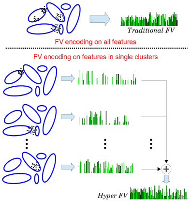
The commonly used Bag-of-Words (BoW) representation [27] consists mainly of feature extraction, generating codebook, feature encoding and pooling, and normalization. Development of well designed low-level features like dense trajectory features [28, 29] and more sophisticated encoding schemes like Fisher vector encoding [20] has resulted in the good performance of BoW model. Though, Fisher vector (FV) encoding [20] is also a variant of BoW model, for clarity purposes, BoW represents (from here on) the Bag-of-Words encoding using k-means clustering. Our proposed work uses the popular improved trajectory features [29] and focuses on improving the encoding of the features to improve the recognition performance. The proposed encoding is based on embedding the BoW encoding into the FV encoding. The proposed encoding is simple and effective and robust to variations in the dictionary size of BoW encoding. This modification can be used in general for other applications, apart from action recognition, which use FV encoding for descriptor computation. The framework of the approach in comparison to the traditional FV encoding is illustrated in figure 1.

1.1 Related Work

Predominantly, there have been many methods to classify actions using low-level features based on space-time interest points (STIP) using various detectors based on Harris3D [12], separable Gabor filters [5], etc. The local features describing the interest points are generally based on gradient information, optical flow [5, 13, 24, 30], local trinary patterns [32], 3D-SIFT [25]. Few of the other approaches include space-time shape representations [8] and template-based methods [2, 6, 22, 23].

In recent years, the trajectory-based methods to perform action classification have become popular and are presented in [1, 15, 31, 10, 28, 29]. Ali et al. [1] used chaotic invariants as features on manually obtained trajectories to recognize actions. Harris3D interest points are tracked and temporal velocity histories of trajectories are used as features by Messing et al. [16]. Matikainen et al. [15] used sparse trajectories from KLT tracker with elements of affine matrices in bag-of-words context as features. However, the performance of dense trajectories is observed to be better than sparse trajectories [31, 29]. Wang et al. [28] use local 3D volume descriptors based on motion boundary histograms (MBH) [4], histogram of oriented gradients (HOG) and histogram of optical flow (HOF) around dense trajectories to encode action. Recently in [29], Wang et al. estimate the camera motion and compensate for it and thereby improving the trajectories and the associated descriptors. The interactions between the dense motion trajectories in an action are quantified and used for recognising actions in [10, 17].

Related to our work of encoding features, Peng et al. [19] give a comprehensive study of the fusion methods for different encoding schemes for action recognition. They evaluate the performance of different encodings, pooling and normalization strategies and fusion methods. Three kinds of fusion levels, viz., descriptor-level, representation-level and score-level fusion are studied. A hybrid representation of fusing outputs from different encodings is also given. Of the three fusion methods, representation-level fusion is closer to our proposed work. The representation-level fusion and the fusion used in hybrid representation are outside of the encoding schemes, unlike in this work, where we are incorporating one encoding (BoW) with in another encoding (FV).

The contribution of this paper is a novel and effective Fisher Vector encoding which performs better than the traditional Fisher Vector encoding. Organization of the rest of the paper is as follows. The Hyper-Fisher Vector encoding for action representation is explained in Section 2. The details of Experimental setup are provided in Section 3. Results on various datasets for action recognition and experiments related to the robustness of the Hyper-Fisher Vector encoding are given in Section 4 and we conclude the paper in Section 5.

2 Hyper-Fisher Vector Encoding

In this section, the proposed Hyper-Fisher Vector encoding is detailed. At first, Fisher Vectors are explained briefly in section 2.1.

2.1 Fisher Vectors

Derived from Fisher kernel, Fisher Vector (FV) coding method was originally proposed for large scale image categorization [20]. The assumption in FV encoding is that the generation process of local descriptors $\mathbf{X}$ can be modeled by a probability density function $p(\textperiodcentered;\theta)$ with parameters $\theta$. The contribution of a parameter to the generation process of $\mathbf{X}$ can be described by the gradient of the log-likelihood with respect to that parameter. Then the video can be described by

$$G_{\theta}^{\mathbf{X}}=\frac{1}{N}\nabla_{\theta}\log p(\mathbf{X};\theta)$$ (1)

The probability density function is usually modeled by Gaussian Mixture Model (GMM), and $\theta=\{\pi_{k},\mu_{k},\sigma_{k}:k=1\ldots K\}$ are the model parameters denoting the mixture weights, means, and diagonal covariances of GMM. $K$ and $N$ are the mixture number and the number of local features, respectively. $\mathbf{X}$ denotes spatial-temporal local features in action videos. Perronnin et al. [20] proposed an improved Fisher vector as follows,

$$v_{\mu,k}=\frac{1}{N\sqrt{\pi_{k}}}\sum_{i=1}^{N}{q_{i}(k)\Bigg{(}\frac{\mathbf{x_{i}}-\mu_{k}}{\sigma_{k}}\Bigg{)}}$$ (2)

$$v_{\sigma,k}=\frac{1}{N\sqrt{2\pi_{k}}}\sum_{i=1}^{N}{q_{i}(k)\Bigg{(}\frac{(\mathbf{x_{i}}-\mu_{k})^{2}}{\sigma_{k}}-1\Bigg{)}}$$ (3)

where $q_{i}(k)$ is the posterior probability associating $\mathbf{x}_{i}$ to the $k$ Gaussian and is given by,

$$q_{i}(k)=\frac{\pi_{k}\mathcal{N}(\mathbf{x}_{i};\mu_{k},\Sigma_{k})}{\sum_{n=1}^{K}{\pi_{n}\mathcal{N}(\mathbf{x}_{i};\mu_{n},\Sigma_{n})}}$$ (4)

The final Fisher vector is the concatenation of all $v_{\mu,k}$ and $v_{\sigma,k}$ and is of $2Kd$ dimension. Power normalization followed by $l_{2}$ normalization is applied to the FV and it gives the best performance on image classification [3] and video-based action recognition [29].

Figure 2: Illustration of the difference in the energy distribution in Hyper Fisher Vector and traditional Fisher Vector via a toy example (see section 2.3 for details). The HFV retains the individual energy maps of LFVs better and hence is more loyal to the contribution of different feature clusters. In comparison, the traditional FV is biased towards the contribution of some features in the set.

2.2 Constructing Hyper-Fisher Vector

The FV encoding results in high-dimensional feature vectors with less number of Gaussians in the mixture and thus yields performance improvement when linear classifiers are used. However, the traditional FV encoding aggregates the local features of an action video by sum pooling over the entire video. Such a representation cannot directly represent higher complex structures. One way to alleviate this shortcoming is to use local pooling and then pool the intermediate FVs. This global-local approach improves the performance of the FV encoding.

The framework of our approach in comparison to the traditional FV encoding is illustrated in figure 1. Let $\mathbf{X}=(\mathbf{x}_{1},\mathbf{x}_{2},\ldots,\mathbf{x}_{N})\in\mathbb{R}^{d\times N}$ be the local features (e.g. HOF, HOG, MBH) obtained from the video of size $W\times H\times L$. Then we compute the $k$-means cluster memberships for each feature $\mathbf{x}_{i}$ using a pre-learned dictionary codebook of size $K_{1}$ from the training set. Let $C=(c_{1},c_{2},\ldots,c_{N})$ be the cluster memberships of the features $\mathbf{X}$. Let there be $k_{c}$ clusters with non-zero members out of $K_{1}$ clusters. For each non-zero cluster, local Fisher Vectors, denoted by $LFV_{i}$ ($i=1\ldots k_{c}$), are computed using a pre-learned GMM with mixture size $K_{2}$ in training set. The local Fisher Vectors are summed to result in the Hyper-Fisher Vector (denoted by $HFV$) representation of the video. The $HFV$ is power normalized and $l_{2}$ normalized as in the case of traditional FV. The LFVs and the HFV are of length $2K_{2}d$.

Algorithm 1 gives the pseudocode for computing the HFV descriptors for a video. $\mu$, $\Sigma$, $\pi$ in the psuedocode represent the mean, diagonal covariances and mixing probabilities of the Gaussians in the pre-learned mixture. $FisherVectorCompute$ computes the FV representation of the input features using the GMM parameters.

Algorithm 1 Compute Hyper-Fisher vector descriptor

  Input: $\{\mathbf{x}_{i}\}_{i=1}^{N}$, $\{c_{i}\}_{i=1}^{N}$, $K_{1}$, $\mu$, $\Sigma$, $\pi$

  

  Output: $HFV$

  

  Initialize $HFV$ to $\mathbf{0}$

  for  $k=1$ to $K_{1}$ do

     $F=\{\mathbf{x}_{i}$ $|$ $c_{i}=k\}$

     if $F=\phi$ then

        continue

     end if

     $LFV=$ $FisherVectorCompute(F,\mu,\Sigma,\pi)$

     $HFV=$ $HFV+LFV$

  end for

  $Power$ $normalize$ $HFV$

  $l_{2}$ $normalize$ $HFV$

Figure 3: Samples from the datasets. (a)-(e) is from Olympic Sports, (f)-(j) is from Youtube (and UCF$50$) and (k)-(n) is from HMDB$51$ datasets.

2.3 Why Hyper-Fisher Vectors are superior?

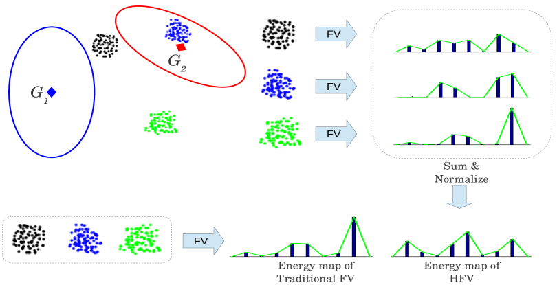
In the last subsection, we showed the approach to construct Hyper-Fisher Vectors. In this subsection, we analyze why the HFVs are superior in comparison to the traditional FVs. We illustrate the difference between the two using a toy example (figure 2). We consider $2$ Gaussians in the mixture and three clusters of features in the feature set. The Gaussians are centered at $(0,0)$ and $(4,4)$ with diagonal variances $(0.5,4)$ and $(0.5,1)$ along $(x,y)$ directions respectively. The three clusters are chosen such that one cluster (centered at $(4,4.5)$ and shown in blue) is well with in one of the Gaussians, the second cluster of features (centered at $(2,2.5)$ and shown in black) is in between the two Gaussians and the third cluster (centered at $(3.5,-0.5)$ and shown in green) is slightly far away from both the Gaussians. All the features are pooled together and the traditional FV representation is obtained. Since we consider $2$ Gaussians in 2$d$ space, the length of the FV is $8$. Standard representation of FV is used where the mean deviation components form the first-half of the FV followed by the variance deviation components.

The energy distribution for the traditional FV among the mean and covariance deviation components is shown in figure 2. For the HFV representation, the clusters are represented by three different LFVs and summed and normalized to obtain the HFV. The energy distributions for each LFV and the HFV are also shown in the figure. The black cluster of features has even distribution of energy among its LFV components and across Gaussians since it is near to both of them. The blue cluster is with in the second Gaussian and hence only those components corresponding to second Gaussian in the associated LFV are high. The green cluster is slightly far from both the Gaussians and has higher energy in the covariance deviation components as compared to the mean deviation components in its LFV. It can be seen that the energy in the covariance deviation components is higher than the mean deviation components in the traditional FV. Whereas, in comparison, the HFV has more energy in its mean deviation components than their counterparts in traditional FV. The energy distribution in HFV is more loyal to the individual distributions in LFVs and hence to the feature clusters. Hence, the HFV represents the feature set better than the traditional FV.

The similarity score (using the linear kernel) between the HFV and the FV shown in the figure is around $0.8$. This depends on the range/width of the clusters. Wider the clusters, higher is the similarity between HFV and FV. Quantitative results on the energy distribution and the similarity between HFV and FV are given in the experimental results section (section  4).

3 Experimental Setup

In this section, the details of the experimental setup with various parameter settings are provided. The datasets used for evaluating the approach are presented in section 3.1.

In the following experiments, improved trajectories and associated descriptors are extracted using the code from Wang [29]. Default parameters are used to extract the trajectories. For the $k$-means clustering (required for HFV encoding), the size of the codebook is chosen to be $4000$ and is learnt using randomly sampled $100,000$ features. For the traditional FV and HFV encodings, the dimensionality of these descriptors is reduced by half using PCA. For the traditional FV, a GMM of size $256$ is learnt using randomly sampled $100,000$ features. The same GMM is used for HFV encoding as well. A linear SVM is used for classification. We use a one-vs-all approach while training the multi-class classifier.

The baseline for our Hyper-Fisher Vector encoding is the traditional Fisher Vector encoding. We also experiment with different power normalizations for the traditional FV encoding and compare against the proposed encoding.

3.1 Datasets

We perform the experiments on four action recognition datasets and report the results. The datasets used for evaluating our work are Olympics Sports, UCF$11$ (also called Youtube dataset), UCF$50$ and HMDB$51$. Few samples from the datasets are shown in figure 3.

The Olympic Sports dataset [18] contains videos of athletes practicing different sports collected from Youtube. It contains $16$ sports action categories and over $750$ videos. Some of the classes are bowling, high jump, shot put, tennis serve. We use the test-train splits provided by the authors for evaluation and report the mAP over all the classes.

Method	Olympic Sports	Youtube	UCF$50$	HMDB$51$
FV	91.1%	90.7%	91.2%	57.2%
FV ($p<0.5$)	91.7%	91.8%	92.1%	58.5%
Hyper FV	92.8%	92.9%	93.0%	60.1%

Table 1: Performance comparison on the three datasets using baseline FV and the proposed Hyper-FV encodings. $p<0.5$ indicates stronger power normalization used for encoding.

The Youtube dataset [14] is collected from YouTube videos. It contains $11$ action categories. Some of the actions are basketball shooting, riding horse, cycling, walking (with a dog). A total of $1,168$ video clips are available. As in [14], we use Leave-One-Group-Out cross-validation and report the average accuracy over all classes.

The UCF$50$ dataset [21] is an extension of the Youtube dataset and contains a total of $6618$ clips from $50$ action categories. We apply the Leave-One-Group-Out cross-validation ($25$ cross-validations) as suggested by the authors [21] and report the average accuracy over all classes.

The HMDB51 action dataset [11] is collected from various sources, mostly from movies, and from public databases such as YouTube and Google videos. The dataset contains $6766$ clips categorized into $51$ action classes, each containing a minimum of $101$ clips. The action categories can be grouped into general facial actions, general body movements with and without object interactions and human interactions. We use the original $3$ train-test splits provided by the authors for evaluation. Each split contains $70$ videos and $30$ videos from every class for training for testing respectively. The average classification accuracy over the three splits is reported.

4 Experimental Results

We conduct different experiments over the datasets to evaluate the performance of the proposed encoding. The results of the experiments Hyper-FV encoding are tabulated in Table 1. The traditional FV encoding is the baseline for the Hyper-FV encoding. Since, the HFV encoding involves two power normalizations, we also compare against the traditional FV encoding with stronger power normalizations ($p<0.5$).

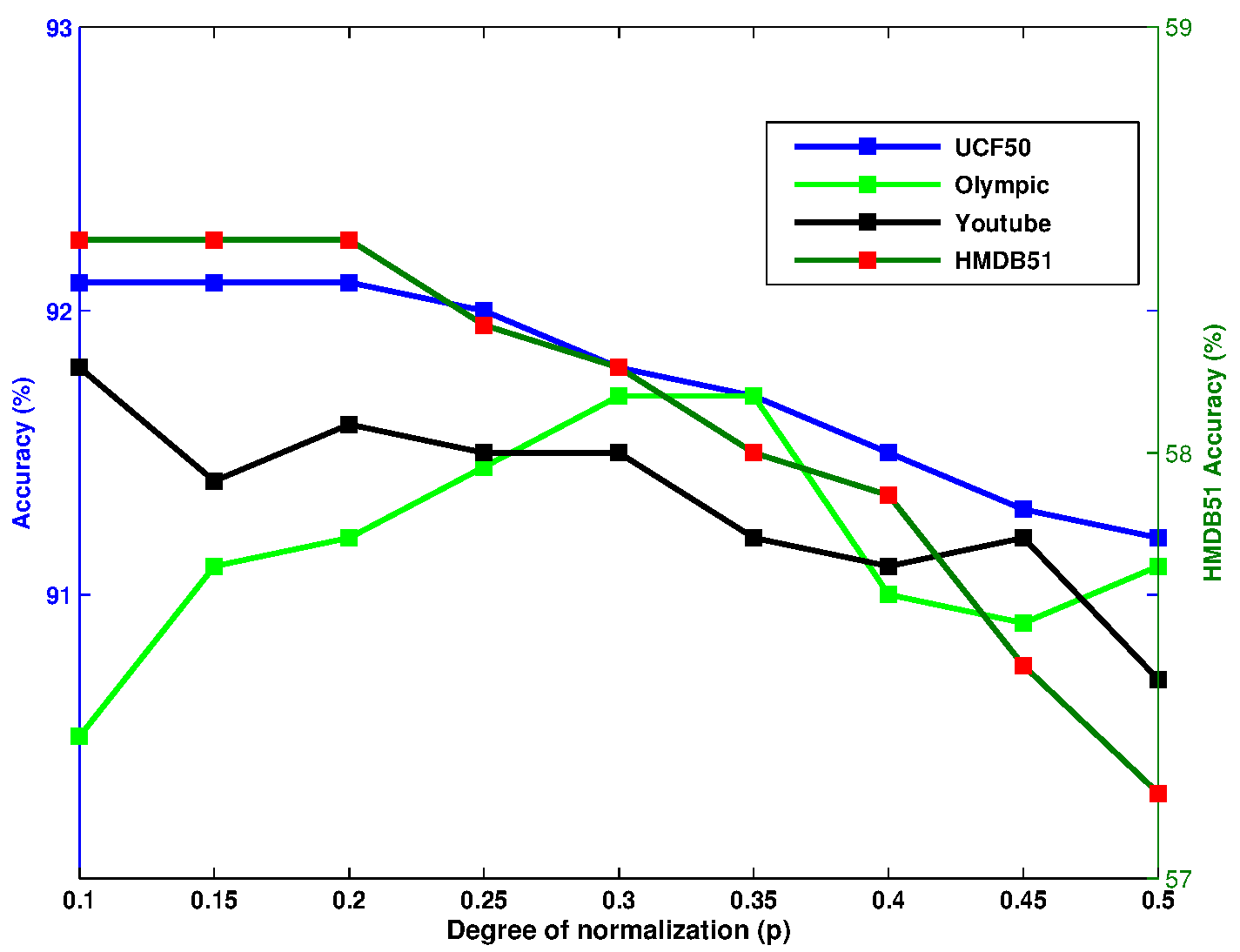
We observe from table 1 that Hyper-FV performs better compared to the traditional FV encoding on all the datasets. The improvement is around $2\%$ for the Olympic Sports, Youtube and UCF$50$ datasets and $3\%$ for HMDB$51$ dataset. The performance of the FV encoding also improves when a stronger power normalization is used. The table 1 reports the best performance for each dataset when $p<0.5$. Figure 4 shows the variation in the performance of FV encoding as the normalization power is varied. Except for Olympic Sports dataset, the accuracy improves as we decrease $p$ from $0.5$ to $0.1$ and the best performance is achieved when $p$ is in the range $0.1$ to $0.2$. For the Olympic Sports dataset, the maximum is reached for $p=0.35$ below which the accuracy decreases. Even though there is an improvement in the performance when a stronger power normalization is used, the performance of the HFV encoding is still better, in general, by $1-1.5\%$ for the four datasets as noted from table 1. This shows that a simple modification in the way the Fisher Vectors are encoded can improve the performance on challenging datasets like UCF$50$ and HMDB$51$.

Figure 4: Plots showing the variation of the performance of FV encoding as the degree of power normalization is varied (HMDB$51$ accuracy on the right $y$-axis).

Figure 5: Plots showing the proportion of the unit energy in mean deviation components of FV and HFV encoding is shown in red and blue respectively. The green curve shows the similarity measure between FV and corresponding HFV of videos in the datasets. The $y$-axis is the number of videos in the datasets (best viewed when zoomed).

Figure 5 shows three plots. Each plot has three functions plotted. The red curve depicts the number of videos in the dataset having different energy proportions in the mean deviation components of the Fisher vector representation of the video. The blue curve depicts the same for the Hyper-Fisher vector representation. Since the total energy in the Fisher vectors sums to $1$, the remaining energy is present in the covariance deviation components of the respective representations. We can observe that the HFV representation in general has mean deviation components with broader energy range than the corresponding FV representations of the videos. The FV red curves are more sharper than the HFV blue curves for each dataset. This shows that the HFV representation has better variations in its components and represents the video actions better. The third curve (in green) shows the similarity scores range for the videos in the dataset. The similarity scores are between corresponding FV and HFV of the videos. The green curve indicates that more than $50\%$ of the videos in the HMDB$51$ dataset have their FV-HFV similarity less than $0.85$. For the Youtube dataset, the similarity scores are centered around $0.7$. This indicates the difference in the representations.

4.1 Robustness of HFV encoding

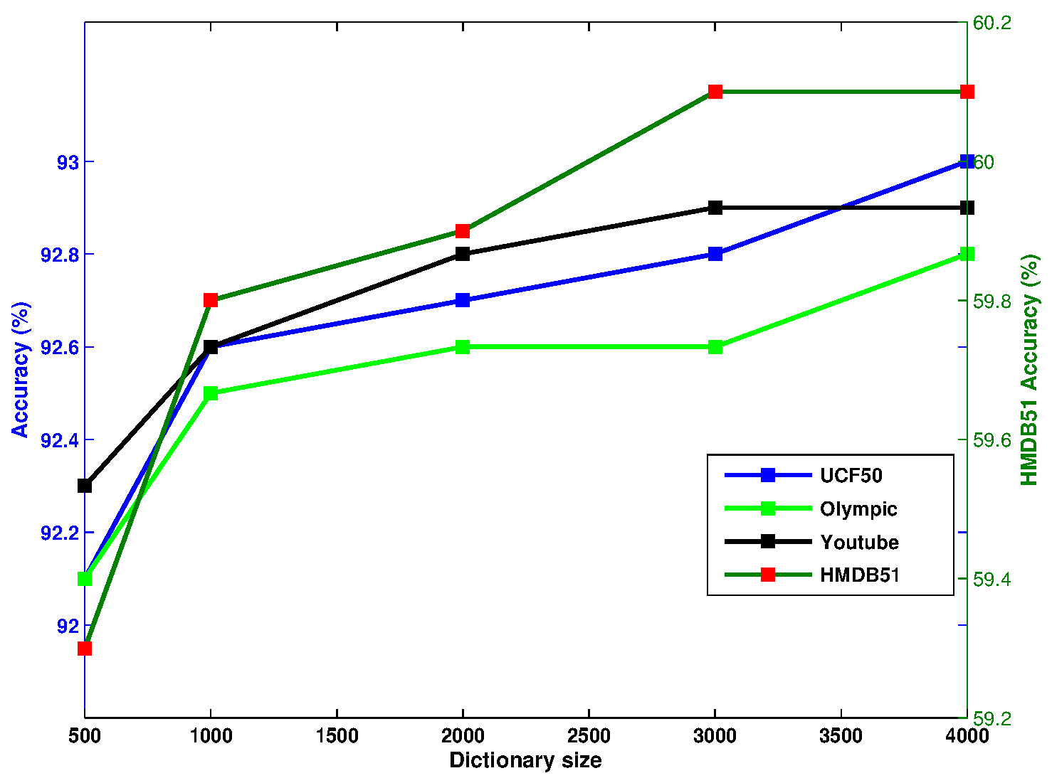
We conduct experiments to test the robustness of the proposed Hyper-FV encoding. The dictionary size of the $k$-means clustering is varied and the performance of the HFV on the datasets is plotted. Figure 6 shows the variation of performance of the HFV encoding as a function of the dictionary size. The dictionary size is varied from $500$ to $4000$. We can see that the accuracy variation is marginal (within $1$ percent) and the HFV encoding performs well even with lower codebook sizes. This shows that the HFV encoding is robust to the codebook size.

Figure 6: Plots showing the variation of the performance of Hyper-FV encoding as the codebook size is varied (HMDB$51$ accuracy on the right $y$-axis).

4.2 Comparison with approaches in literature

We compare the results of our method with the recent results reported in literature for each dataset. It is tabulated in table 2. For the purpose of a fair comparison, approaches involving deep networks for action recognition are not compared here. The improvements for Olympic Sports, Youtube and UCF$50$ datasets are around $2\%$ and our method improved the performance on the more challenging HMDB$51$ dataset by $3\%$ in comparison to the other approaches. In particular, Wang et al. [29] use the Fisher Vector encoding and in comparison, the proposed encoding performs better. This shows that our HFV encoding can be used to substitute the original FV encoding for improved performance in various applications.

Olympic Sports		Youtube		UCF$50$		HMDB$51$
Gaidon et al. [7]	82.7%	Wang et al. [28]	85.4%	Wang et al. [28]	84.5%	Wang et al. [28]	46.6%
Jain et al. [9]	83.2%	Liu et al. [14]	71.2%	Shi et al. [26]	83.3%	Zhu et al.	54.0%
iDT+FV [29]	91.1%	iDT+FV [29]	90.7%	iDT+FV [29]	91.2%	iDT+FV [29]	57.2%
Proposed	92.8%	Proposed	92.9%	Proposed	93.0%	Proposed	60.1%

Table 2: Comparison of our proposed approach with other approaches on Olympic Sports, Youtube, UCF$50$ and HMDB$51$ datasets.

5 Conclusion

In conclusion, we have developed a novel Hyper-Fisher Vector encoding which embeds the Bag-of-Words encoding into the Fisher Vector encoding. In this work, the Hyper-FV encoding has been used to represent actions in videos. We evaluated our approaches on challenging datasets such as UCF$50$ and HMDB$51$ and the Hyper-FV encoding was shown to perform better than the FV encoding. Thus the proposed encoding can be used in place of the FV encoding in different applications for better representation and can also be used in deep networks, such as deep Fisher networks for action recognition.

References

- [1] S. Ali, A. Basharat, and M. Shah. Chaotic invariants for human action recognition. In ICCV, 2007.
- [2] A. Bobick and J. Davis. The recognition of human movement using temporal templates. TPAMI, 23(3):257–267, 2001.
- [3] K. Chatfield, V. Lempitsky, A. Vedaldi, and A. Zisserman. The devil is in the details: an evaluation of recent feature encoding methods. In BMVC, 2011.
- [4] N. Dalal, B. Triggs, and C. Schmid. Human detection using oriented histograms of flow and appearance. In ECCV, 2006.
- [5] P. Dollar, V. Rabaud, G. Cottrell, and S. Belongie. Behavior a recognition via sparse spatio-temporal feature. In VS-PETS, 2005.
- [6] A. A. Efros, A. Berg, G. Mori, and J. Malik. Recognizing action at a distance. In ICCV, 2003.
- [7] A. Gaidon, Z. Harchaoui, and C. Schmid. Recognizing activities with cluster-trees of tracklets. In BMVC, 2012.
- [8] L. Gorelick, M. Blank, E. Shechtman, M. Irani, and R. Basri. Actions as space-time shapes. TPAMI, 29(12):2247–2253, 2007.
- [9] M. Jain, H. Jégou, and P. Bouthemy. Better exploiting motion for better action recognition. In CVPR, 2013.
- [10] Y.-G. Jiang, Q. Dai, X. Xue, W. Liu, and C.-W. Ngo. Trajectory-based modeling of human actions with motion reference points. In ECCV, 2012.
- [11] H. Kuehne, H. Jhuang, E. Garrote, T. Poggio, and T. Serre. Hmdb: a large video database for human motion recognition. In ICCV, 2011.
- [12] I. Laptev and T. Lindberg. Space-time interest points. In ICCV, 2003.
- [13] I. Laptev, M. Marszalek, C. Schmid, and B. Rozenfeld. Learning realistic human actions from movies. In CVPR, 2008.
- [14] J. Liu, L. Luo, and M. Shah. Recognizing realistic actions from videos “in the wild”. In CVPR, 2009.
- [15] P. Matikainen, M. Hebert, and R. Sukthankar. Trajectons: action recognition through the motion analysis of tracked features. In ICCV Workshop, 2009.
- [16] R. Messing, C. Pal, and H. Kautz. Activity recognition using the velocity histories of tracked keypoints. In ICCV, 2009.
- [17] S. Narayan and K. R. Ramakrishnan. A cause and effect analysis of motion trajectories for modeling actions. In CVPR, 2014.
- [18] J. C. Niebles, C.-W. Chen, and L. Fei-Fei. Modeling temporal structure of decomposable motion segments for activity classification. In ECCV. 2010.
- [19] X. Peng, L. Wang, X. Wang, and Y. Qiao. Bag of visual words and fusion methods for action recognition: Comprehensive study and good practice. arXiv preprint arXiv:1405.4506, 2014.
- [20] F. Perronnin, J. Sánchez, and T. Mensink. Improving the fisher kernel for large-scale image classification. In ECCV, 2010.
- [21] K. K. Reddy and M. Shah. Recognizing 50 human action categories of web videos. Machine Vision and Applications, pages 1–11, 2012.
- [22] M. Rodriguez, J. Ahmed, and M. Shah. Action mach: a spatio-temporal maximum average correlation height filter for action recognition. In CVPR, 2008.
- [23] S. Sadanand and J. J. Corso. Action bank: A high-level representation of activity in video. In CVPR, 2012.
- [24] C. Schuldt, I. Laptev, and C. B. Recognizing human actions: A local SVM approach. In ICPR, 2004.
- [25] P. Scovanner, S. Ali, and M. Shah. A 3-dimensional sift descriptor and its application to action recognition. In ACM Multimedia, 2007.
- [26] F. Shi, E. Petriu, and R. Laganiere. Sampling strategies for real-time action recognition. In CVPR, 2013.
- [27] J. Sivic and A. Zisserman. Video google: A text retrieval approach to object matching in videos. In ICCV, 2003.
- [28] H. Wang, A. Kläser, C. Schmid, and C.-L. Liu. Dense trajectories and motion boundary descriptors for action recognition. IJCV, pages 1–20, 2013.
- [29] H. Wang and C. Schmid. Action Recognition with Improved Trajectories. In ICCV, 2013.
- [30] H. Wang, M. M. Ullah, A. Klaser, I. Laptev, and C. Schmid. Evaluation of local spatio-temporal features for action recognition. In BMVC, 2009.
- [31] S. Wu, O. Oreifej, and M. Shah. Action recognition in videos acquired by a moving camera using motion decomposition of lagrangian particle trajectories. In ICCV, 2011.
- [32] L. Yeffet and L. Wolf. Local trinary patterns for human action recognition. In ICCV, 2009.