Primordial gravitational waves and the collapse of the wave function

Abstract

“The self-induced collapse hypothesis” was introduced by D. Sudarsky and collaborators to explain the origin of cosmic structure from a perfect isotropic and homogeneous universe during the inflationary regime. In this paper, we calculate the power spectrum for the tensor modes, within the semiclassical gravity approximation, with the additional hypothesis of a generic self-induced collapse of the inflaton’s wave function; we also compute an estimate for the tensor-to-scalar ratio. Based on this calculation, we show that the considered proposal exhibits a strong suppression of the tensor modes amplitude; nevertheless, the corresponding amplitude is still consistent with the joint BICEP/KECK and Planck Collaboration’s limit on the tensor-to-scalar ratio.

I Introduction

Observations of the Cosmic Microwave Background (CMB) radiation are one of the most powerful tools to study the early universe. Before the formation of neutral hydrogen, photons and electrons were coupled by Thomson scattering. Once photons were decoupled from matter, they traveled freely through the universe almost without interacting with matter. Accordingly, the CMB radiation provides information about the physical parameters of the universe at recombination and also about the content of matter and energy density inside it. In the past two decades there has been a major improvement in the measurement of CMB fluctuations: a large number of experiments have been performed including a mix of of ground-, balloon- and space-based receivers.

Furthermore, from the estimation of the spectrum of initial perturbations, the CMB spectrum also provides an indirect evidence of the early universe physics. Different inflationary models proposed in the literature make distinct predictions of the primordial spectrum Martin et al. (2014a, b) and, thus, the CMB radiation is an excellent observational tool to test them. Temperature fluctuations are the result of perturbations in the gravitational potentials, which contribute directly to the fluctuations via gravitational red-shifting and which also drive acoustic oscillations of the primordial plasma. These processes result in temperature fluctuations that are of the same order of magnitude as the metric perturbations. On the contrary, CMB polarization is not directly generated by metric perturbations: a net polarization arises from Compton scattering only when the incident radiation field possesses a non-zero quadrupole moment. Polarization is only originated very near to the last scattering surface as the photons begin to decouple from the electrons generating a quadrupole moment through free-streaming. The tensor nature of CMB polarization allows a separation of scalar fluctuations from tensor ones. CMB polarization maps can be decomposed into two terms: often-called $E$ and $B$-modes in analogy with the electric and magnetic field. Gravitational waves generated during inflation, in contrast to adiabatic scalar perturbations, imprint a unique divergence-free pattern of polarization on the sky, namely, the $B$-mode. Scalar perturbations have no handedness so the $B$-mode component at low angular multipole scales exists only if there is a tensor perturbation generated by primordial gravitational waves. On the other hand, detection of $B$-modes at large angular multipoles has been reported by the Polarbear experiment The Polarbear Collaboration: P. A. R. Ade et al. (2014). However, it is known, that the source for this detection is gravitational lensing of the CMB radiation. In such a way, the detection of the $B$-mode signal at low angular multipoles provides the cleanest window into the unique predictions of the inflationary cosmological paradigm.

Last year, the BICEP collaboration reported a measurement of the $B$-mode polarization consistent with the prediction of standard inflationary models with tensor modes Ade et al. (2014). However, it was pointed out that, without an accurate dust map, it is not possible to discern between dust polarization and polarization due to primordial gravity waves Mortonson and Seljak (2014); Flauger et al. (2014); Liu et al. (2014). In turn, an estimation of the dust present in BICEP2 experiment made by the Planck collaboration (extrapolating information from the 353 GHz map) showed that the detection informed by BICEP2 may be due to dust polarization Planck Collaboration et al. (2014). Finally, a joint analysis of the BICEP/Keck and Planck collaborations BICEP2/Keck and Planck Collaborations et al. (2015) showed that the detection made by the BICEP collaboration is consistent with dust polarization and that there is no statistically significant evidence for tensor modes.

According to the standard inflationary scenario, the onset of all cosmic structures is explained by considering a featureless stage described by a background Friedmann-Robertson-Walker (FRW) cosmology with a nearly exponential expansion driven by the potential of a single scalar field. Additionally, the field’s quantum fluctuations are characterized by a simple vacuum state, which is homogeneous and isotropic (for a proof of this statement see Appendix A of Ref. Landau et al. (2013)). In particular, the quantum fluctuations transmute into the classical statistical fluctuations that represent the seeds of the current cosmic structure like galaxies and galaxy clusters. However, there is an issue regarding the usual explanation for the origin of cosmic structure; this is, the standard inflationary paradigm lacks a physical mechanism capable of generating the inhomogeneity and anisotropy of our universe, from an exactly homogeneous and isotropic initial state characterizing both: the background space-time and the quantum state of the inflaton. This problem has been analyzed in previous works Perez et al. (2006); Sudarsky (2011); Landau et al. (2013) and one key aspect of the problem is that there is no satisfactory solution within the standard physical paradigms of quantum unitary evolution because this kind of dynamics is not capable to break the initial symmetries of the system. To handle this shortcoming, a proposal has been developed by D. Sudarsky and collaborators Perez et al. (2006); Sudarsky (2007); de Unánue and Sudarsky (2008); León and Sudarsky (2010); León et al. (2011); Diez-Tejedor and Sudarsky (2012); Landau et al. (2012); Cañate et al. (2013); Landau et al. (2013); León et al. (2014); León and Sudarsky (2015). In this scheme, a new ingredient is introduced into the inflationary scenario: the self-induced collapse hypothesis. The main assumption is that, at a certain stage in the cosmological evolution, there is an induced jump from the original quantum state characterizing the particular mode of the quantum field; after the jump, the quantum state is inhomogeneous and anisotropic, namely, it must not be an eigen-state of the linear and angular momentum operators. Therefore, by considering a self-induced collapse (in each mode) of the inflaton wave function, the inhomogeneities and anisotropies emerge at each particular length scale, i.e. the quantum collapse acts a source for the primordial curvature perturbation. As a consequence of this modification to the inflationary scenario, the predicted primordial power spectrum is changed as well as the CMB fluctuation spectrum. Previous works Perez et al. (2006); Sudarsky (2011); Landau et al. (2013); Diez-Tejedor and Sudarsky (2012) have extensively discussed both the conceptual and formal aspects of this new proposal, and we refer the reader to the references. In this paper, motivated by the discussion generated around BICEP2’s claim, we compute the tensor power spectrum and the tensor-to-scalar ratio corresponding to the amplitude of primordial gravitational waves resulting from considering a generic self-induced collapse. Furthermore, in the theoretical framework of the self-induced collapse, the inflationary era is more accurately described by the semiclassical Einstein equations, namely, the perturbations of the scalar field are quantized and the metric perturbations remain always classical. In this paper, we calculate the prediction for tensor primordial power spectrum generated by gravitational waves and find that the self-induced collapse hypothesis, plus semiclassical gravity, predicts a strong suppression of the amplitude of the tensor modes.

It is worthwhile to mention that our result is consistent with the findings presented in Ref. Markkanen et al. (2015), i.e. that the semiclassical gravity approximation plus a collapse of the inflaton’s wave function lead those authors to qualitatively argue that the amplitude of the primordial gravitational waves is undetectable; however, those authors consider a possible non-minimally coupling between gravity and the inflaton, and also that the state collapses on a spacelike hypersurface for all wavelengths modes, this contrasts with our view in which the time of collapse depends on the mode’s wavelength. Also, in the present manuscript, we provide a detailed calculation of the tensor-to-scalar ratio (in Ref. Markkanen et al. (2015) the calculations involved only scalar perturbations).

The paper is organized as follows: In Section II, we review the semiclassical gravity approximation and its relation with the self-induced collapse; in Section III, we briefly review the proposal of the collapse of the wave function in the case where only scalar perturbations were considered; in Section IV, we present how the scalar perturbations, generated by the self-induced collapse, originates the tensor modes; in Section V, we compute the power spectrum for the tensor modes; in Section VI we provide an estimate of the tensor-to-scalar ratio, and finally in Section VII, we present our conclusions. We have also included an Appendix section in which we present the explicit form of some functions used in the calculations.

II The semiclassical gravity approximation and the collapse of the wave function

Our analysis of the inflationary universe considers the corresponding regime in a way that a quantum treatment of the matter fields is appropriate, while a classical description of gravitation would be justified simply because the measures of curvature are all well below the Planck scale. That is the realm of semiclassical gravity characterized by ($c=1$):

$$G_{ab}=8\pi G\langle\hat{T}_{ab}\rangle.$$ (1)

The left hand side of this equation, namely the Einstein’s tensor, contains the gravitational degrees of freedom that are always treated in a classical way. The right hand side, is the expectation value of a quantum operator, $\hat{T}_{ab}$ describing the quantum matter degrees of freedom.

Let us consider first how a self-induced collapse of the wave function fits into the semiclassical gravity framework (extended discussion can be found in Refs. Diez-Tejedor et al. (2012); Diez-Tejedor and Sudarsky (2012)). It is known, that gravity is perhaps the most complicated component of our universe to fit with the general paradigms offered by a quantum theory. There exists an extensive literature on this subject and the present manuscript does not even attempt to describe all the technical and/or conceptual problems associated with it. However, one aspect to consider is that, according to general relativity, the structure of the space-time is the core of gravitation, meanwhile, quantum theory seems to fit most easily in contexts where the space-time is already present (or given). In other words, quantum states are associated with objects that “live” in space-times. Evidently, deep conceptual modifications are in order if one aspires to provide a characterization of space-time itself in a quantum language. For instance, the canonical approach to quantum gravity DeWitt (1967); Giulini and Kiefer (2007), suffers from the so called problem of time Isham (1992). It seems thus natural to speculate that in this setting a dramatic departure from the quantum orthodoxy, such as a dynamical reduction of the wave function might find its origin, i.e. it is possible that a more fundamental description of quantum gravity would take the form of deviations form the standard unitary evolution that characterize quantum theory as we know it (for a particular example how these ideas can be implemented in the black hole information paradox see Refs. Okon and Sudarsky (2015); Modak et al. (2015a, b)).

In other words, it seems a plausible conjecture that a variation of standard quantum theory, that we have referred to here as described effectively by the “collapse of the wave function,” corresponds to lasting features of the fundamental timeless (and probably spaceless) theory of quantum gravity. If that is the case, the emergence of space-time itself would be tied to the incorporation of such effective quantum description of matter fields living on a space-time, and evolving approximately according to standard quantum field theory on curved spaces, with some small deviations that might include our collapse hypothesis. Similar ideas of this kind regarding gravity as an emergent phenomenon have been considered previously (e.g. Refs. Jacobson and Hu (1993); Ashtekar (2013)). This seems to suggest that, in the context where we consider the collapse of the wave function, the space-time itself must be considered as an approximate phenomenological characterization, and, therefore, something that cannot be subjected to quantization. For a more pictorial example, we can consider the following analogy: the propagation of heat in a medium. This phenomenon can be described by the heat equation $\partial T/\partial t-\nabla^{2}T=S$, where $T$ is the temperature of the medium and $S$ the heat sources. It is quite clear that despite the fact that this equation resembles an equation for some field, it would be meaningless to quantize it. Furthermore, we can consider some situation in which the source of heat requires a quantum mechanical treatment, i.e. taking $S$ as a quantum operator. Under such conditions, it seems natural that to the extent that the temperature description is still relevant and of interest, the right hand side of the equation above should be replaced by something like $\langle\hat{S}\rangle$. Evidently, there will be situations that are so far removed from the context where the heat equation was derived that even the notion of temperature itself would become meaningless. We equally expect that in the fundamental quantum theory of gravity we will be able to find several situations where the semiclassical gravity approximation would fail completely, but in following with our line of thought and previous analogy, it seems quite possible that those would correspond to situations where the concept of space-time itself becomes meaningless.

Clearly, all these arguments above are filled with “educated guesses” and conjectures, and we only take them as guidances. Nevertheless, as we will show in the rest of this manuscript, when considering these ideas within the context of the inflationary universe and, in particular, using them to analyze the emergence of primordial gravitational waves, we are able to provide an observational constraint. If it happens that our proposal does not match the observational data, then clearly we should find another way to incorporate our self-induced collapse proposal in the traditional inflationary setting, namely, the one involving the quantization of metric perturbations (some preliminary steps in that direction can be found in Refs. Mariani et al. (2014); Leon and Bengochea (2015)).

After the previous digression, we turn our focus on the generation of the primordial perturbations provided by the self-induced collapse.

The starting point provided by inflation corresponds to an homogeneous and isotropic state for the gravitational and matter degrees of freedom; this is, the background space-time is symmetric and the quantum state characterizing the inflaton is an eigen-state of the linear and angular momentum operators. The self-induced collapse proposal, states that at some stage during inflation, the quantum state of the matter fields, normally associated to the inflaton, undergoes a spontaneous collapse (evidently without relying on any external entities such as “observers,” “measurement devices,” etc.). The resulting state of the matter fields no longer needs to share the symmetries of the initial state, and, its coupling to the gravitational degrees of freedom, through Einstein’s semiclassical equation, leads to a geometry that is no longer homogeneous and isotropic. Thus, the quantum collapse acts as a source for the inhomogeneities and anisotropies in the universe, this is the main role for introducing the collapse of the wave function.

The idea of a self-induced collapse of the wavefunction, in a non-cosmological setting, has been analyzed in great detail in the past (for a review of objective collapse models see Ref. Bassi and Ghirardi (2003)). Furthermore, R. Penrose and L. Diósi have long advocated to gravity as the main agent triggering the collapse Penrose (1996); Diosi (1987); the reasoning is that a self-induced collapse occurs when the matter fields are in a quantum superposition that would lead to corresponding space-time geometries that are “too distinct among themselves.” This kind of gravity-induced collapse would be happening in fairly common situations, providing a resolution of the measurement problem in quantum mechanics. In our view, which can be thought as an attempt to apply these ideas to the cosmological context, in order to address the shortcoming mentioned in the Introduction, the present formalism must be regarded as an effective description of the fundamental collapse mechanism, possibly as consequence of a successful quantum gravity theory, which in the present situation leads to a transition from the symmetric vacuum state to the non-symmetrical latter state (the symmetry being homogeneity and isotropy). We will not discuss further these motivations here and instead our analysis should be regarded as a purely phenomenological scheme, in the sense that it does not seek to provide a physical mechanism for the collapse, but merely to present a generic parametrization of the collapse. The main formalism and conceptual framework can be consulted in Refs. Perez et al. (2006); Sudarsky (2011); Landau et al. (2013); Diez-Tejedor and Sudarsky (2012).

There is also an issue regarding the semiclassical approximation during the collapse. It is well known that introducing a dynamical collapse generically violates the conservation of energy, so the divergence of the energy-momentum tensor $\nabla_{a}\langle\hat{T}^{ab}\rangle$ does not vanish. If that happens, then of course the divergence of the Einstein tensor does not vanish either, which evidently is a problem since we know that this divergence must be zero. Therefore, during the collapse, we cannot say how the modified dynamics, provided by a dynamical reduction of the wave function associated to the quantum fields, affects the classical metric perturbations that are directly related to the observables, that is, the temperature anisotropies. However, this shortcoming does not necessarily mean that we cannot implement a collapse mechanism in our formalism; the semiclassical gravity approximation is valid before and after the collapse and these will be the two regimes of interest for the present work. Before the collapse, the source for the metric perturbations is zero and only after the collapse (where there is no violation of energy conservation) the expectation values of the operator $\hat{T}_{ab}$ evaluated at the post-collapse state, act as a source for the metric perturbations.

As we mentioned, the principal role for the collapse of the wave function is to act as the main agent for breaking the symmetries (homogeneity and isotropy) of the primordial universe. At first-order, the scalar metric perturbations are generated, via the semiclassical approximation, by the expectation value of the matter scalar perturbations in the post-collapse state. Nevertheless, the matter perturbations–at this order–do not act as a source for the tensor metric perturbations, thus, within our model, the amplitude for first-order tensor modes is zero. In turn, second-order tensor modes, can be generated via first-order scalar perturbations (of both metric and matter perturbations) Mollerach and Matarrese (1997); Mollerach (1998); Mollerach et al. (2004); Osano et al. (2007); Ananda et al. (2007); Baumann et al. (2007). As a consequence, one naively expects that the tensor to scalar ratio computed within the semiclassical gravity approximation will be much smaller than the one computed in the standard case. On the other hand, as shown in Refs. Perez et al. (2006); Sudarsky (2007); de Unánue and Sudarsky (2008); León and Sudarsky (2010); León et al. (2011); Diez-Tejedor and Sudarsky (2012); Landau et al. (2012); Cañate et al. (2013); Landau et al. (2013), the self-induced collapse modifies the scalar power spectrum in a very particular way, namely by including a function of the time of collapse, and in principle, we would not know a priori if the same modification to the tensor power spectrum might result in a detectable amplitude of primordial gravitational waves even if the tensor power spectra is generated at second-order in the perturbations. This is different from the standard procedure where the Mukhanov-Sasaki variable (which mixes metric and inflaton’s perturbations) is quantized. In that case, tensor modes are generated at the first-order approximation; however, as analyzed in Refs. Osano et al. (2007); Ananda et al. (2007); Baumann et al. (2007), one can also compute the second-order contribution to the tensor modes provided by scalar perturbations.

We would like to emphasize the fact that tensor perturbations are exactly zero at first-order because we are considering the semiclassical Einstein equations and not because the assumption of a self-induced collapse of the inflaton’s wave function. In fact, in recent papers, one of us has calculated the tensor power spectrum and the tensor-to-scalar ratio working in terms of a joint metric-matter quantization and including the self-induced collapse of the inflaton’s wave function leading to different results as the ones reported here Mariani et al. (2014); Leon and Bengochea (2015). In particular, we will assume that the collapse of the wave function of each mode of the inflaton field has occurred creating first-order scalar metric perturbations; then, we will use such perturbations as a source of second-order tensor modes, i.e. as the origin of the primordial gravitational waves. In the following sections, we will estimate the amplitude of the second-order tensor modes generated by the process described above.

III Inflation and the collapse of the wave function: scalar perturbations

In this section we present a very brief review of the implementation of the collapse proposal to the inflationary universe, in particular, we will focus on the first-order scalar perturbations of the metric. Since this subject has been extensively discussed in previous works Perez et al. (2006); de Unánue and Sudarsky (2008); León and Sudarsky (2010); Sudarsky (2011); Diez-Tejedor and Sudarsky (2012); Landau et al. (2012, 2013), we will only present the main results, and refer to the reader to the aforementioned works for more details.

We start with the standard inflationary model characterized by the action ($c=1$):

$$S[\phi,g_{ab}]=\int d^{4}x\sqrt{-g}\bigg{(}\frac{R[g]}{16\pi G}-\frac{1}{2}\nabla_{a}\phi\nabla^{a}\phi-V[\phi]\bigg{)}.$$ (2)

with $\phi$ a scalar field representing the inflaton. The metric and scalar field are separated into background plus perturbations. The background is represented by a spatially flat FRW space-time with line element $ds^{2}=a(\eta)[-d\eta^{2}+\delta_{ij}dx^{i}dx^{j}]$ and the homogeneous part of the scalar field $\phi_{0}(\eta)$ in the slow-roll regime. The scale factor corresponding to the inflationary era is $a(\eta)\simeq-1/(H\eta)$ with $H$ the Hubble factor which, during inflation, is related to the inflaton potential as $H^{2}\simeq(8\pi G/3)V\simeq$ constant. From these considerations, one infers that the conformal time $\eta$ is in the range $\eta\in(-\infty,\eta_{r})$, where $\eta_{r}$ is very small in absolute terms, $\eta_{r}\simeq-10^{-22}$ Mpc. The slow-roll regime, is characterized by $\phi_{0}^{\prime}\simeq-(a^{3}/3a^{\prime})\partial_{\phi}V$, and the slow-roll parameter is $\epsilon\equiv 1-\mathcal{H}^{\prime}/\mathcal{H}^{2}\simeq\frac{1}{2}M_{P}^{2}(\partial_{\phi}V/V)^{2}\ll 1$; here, a prime denotes partial derivative with respect to conformal time $\eta$ and $M_{P}$ is the reduced Planck’s mass defined as $M_{P}^{2}\equiv 1/(8\pi G)$ ($\hbar=1$). Furthermore, we will work with the approximation $\epsilon=$ constant.

Let us focus on the first-order scalar perturbations, as these will be the ones of interest for the present work. We will be working in the so-called longitudinal gauge, the perturbed metric is, thus, represented by:

$$ds^{2}=a(\eta)^{2}[-(1+2\Phi)d\eta^{2}+(1-2\Psi)\delta_{ij}dx^{i}dx^{j}].$$ (3)

In the absence of anisotropic stress $\Phi=\Psi$. The quantity $\Psi(\vec{x},\eta)$ is called the “Newtonian potential” and it also represents the curvature perturbation in the longitudinal gauge.

Turning our attention to the inflaton’s perturbations, it is convenient to work with the quantum field $\hat{y}=a\hat{\delta\phi}$, and its canonical conjugate momentum $\hat{\pi}=a\hat{\delta\phi}^{\prime}=\hat{y}^{\prime}-\hat{y}a^{\prime}/a$. For each Fourier component of the perturbations, Einstein’s semiclassical equations at first-order $\delta G_{ab}^{(1)}=8\pi G\langle\delta\hat{T}_{ab}^{(1)}\rangle$ yield

$$\Psi_{\textbf{k}}(\eta)=\sqrt{\frac{\epsilon}{2}}\frac{H}{M_{P}k^{2}}\langle\hat{\pi}_{\textbf{k}}(\eta)\rangle.$$ (4)

It is clear from Eq. (4) that if the state of the field is the vacuum state, all modes associated to the metric perturbation vanish, and, thus the space-time is homogeneous and isotropic.

As discussed in Ref. Perez et al. (2006); de Unánue and Sudarsky (2008); León et al. (2011), as a result of the collapse, each mode jumps to a new state $|\Theta\rangle$ characterized by the expectation value of a certain operator, which is determined by the pre-collapse uncertainties and a random number. In the scheme we consider here, the state will be (partially) characterized by:

$$\langle\hat{y}_{\vec{k}}^{R,I}(\eta_{k}^{c})\rangle_{\Theta}=0,\quad\langle\hat{\pi}_{\vec{k}}^{R,I}(\eta_{k}^{c})\rangle_{\Theta}=x_{\vec{k}}^{R,I}\sqrt{[\Delta\hat{\pi}_{\vec{k}}^{R,I}(\eta_{\vec{k}}^{c})]_{0}^{2}},$$ (5)

where $R,I$ denotes the real and imaginary parts of the operators, respectively; $\eta_{\vec{k}}^{c}$ represents the time of collapse for each mode. The pre-collapse state is the Bunch-Davies vacuum and $[\Delta\hat{\pi}_{\vec{k}}^{R,I}]_{0}^{2}$ is the corresponding uncertainty. This scheme is motivated by the fact that the variable which is directly related with the Newtonian potential $\Psi$, is the expectation value of $\hat{\pi}$, but it also serves to simplify, without loss of generality, the second-order calculation of the next section.

The $x_{\textbf{k}}^{R,I}$ are numbers selected randomly from a Gaussian distribution centered at $0$ and with unit dispersion.. In our approach, our universe corresponds to a single realization of these random variables, and, thus, each of these quantities has a single specific value. Some statistical aspects concerning these quantities can be studied using as a tool an imaginary ensemble of “possible universes,” but we should in principle distinguish those from the statistics of such quantities for the particular universe we inhabit.

In terms of the random variables, Eq. (4) can be rewritten as Perez et al. (2006); de Unánue and Sudarsky (2008); León et al. (2011)

$$\Psi_{\textbf{k}}(\eta)=\frac{\sqrt{\epsilon}H}{M_{P}}\left(\frac{L}{2k}\right)^{3/2}\left(\cos[k\eta-z_{k}]+\frac{\sin[k\eta-z_{k}]}{z_{k}}\right)X_{\textbf{k}},$$ (6)

where $X_{\textbf{k}}\equiv x_{\textbf{k}}^{R}+ix_{\textbf{k}}^{I}$, $z_{k}\equiv k\eta_{\vec{k}}^{c}$ and $\eta_{\vec{k}}^{c}$ is the time of collapse of each mode $k$, also $L$ is the side length of the cubic box in which we are performing the quantization of the fields. In other words, the Fourier’s modes $\Psi_{\textbf{k}}$ correspond to $\Psi(\eta,\vec{x})=1/L^{3}\sum_{\textbf{k}\neq 0}\Psi_{\textbf{k}}(\eta)e^{i\textbf{k}\cdot\vec{x}}$, where the sum is over wave vectors k satisfying $k_{i}L=2\pi n_{i}$ for $i=1,2,3$ with $n_{i}$ integer; at the end of calculations we can take the limit $L\to\infty$ thus making k continuous.

This result expresses the Newtonian potential, after the collapse, in terms of the random variables that determine the post-collapse state. One of the advantages of our approach is that the origin of the randomness, which one usually attributes to quantum theory, becomes transparent and specific: the variables $X_{\textbf{k}}$ characterize, once and for all, every kind of stochasticity involved. The Newtonian potential is closely related with the observational quantity i.e., the temperature anisotropies. Therefore, the set of all the random variables $\{X_{\textbf{k}_{1}},X_{\textbf{k}_{2}},X_{\textbf{k}_{3}}\ldots\}$ corresponding to our universe fixes the value of the observed temperature anisotropies. Naturally, we cannot give a definite prediction for those values, however, as we will show next, the fact that a large number of modes $\vec{k}$ contribute to the observed temperatures anisotropies, justifies a statistical analysis that leads to a theoretical estimate for the observational quantities.

Furthermore, $\Psi_{\textbf{k}}$ also depends on the time of collapse $\eta_{\vec{k}}^{c}$ (recall the definition $z_{k}\equiv k\eta_{\vec{k}}^{c}$), which is the additional parameter introduced by our model.

In previous works de Unánue and Sudarsky (2008); Landau et al. (2012) it has been shown that if $z_{k}$ is independent of $k$ our model yields the same prediction for the scalar primordial power spectrum as the standard inflationary models and, thus, the predictions for the CMB temperature, $E$-mode and $TE$ cross-correlation spectrum is also the same as in the standard scenario. In fact, in León et al. (2015), it is shown that the prediction for the scalar power spectrum, which is obtained from Eq. (6), is

$$P_{S}(k,\eta)\simeq\frac{H^{2}}{64\pi^{2}M_{P}^{2}\epsilon}\left(\cos[z_{k}]-\frac{\sin[z_{k}]}{z_{k}}\right)^{2}k^{n_{s}-1}.$$ (7)

Moreover, in Ref. Landau et al. (2012) some of us have also performed a statistical analysis using WMAP 7-year-data together with other CMB data and constrained the possible departures of the assumption $z_{k}$ independent of $k$. On the other hand, this shows that implementing the collapse hypothesis to the inflationary universe, translates into adding a new degree of freedom, namely the time of collapse $\eta_{\vec{k}}^{c}$. Therefore, in what follows, we will assume that $z_{k}$ is a constant which implies $k\eta_{\vec{k}}^{c}=z$ with $z$ a free parameter of the collapse model. In other words, the relation between $k$ and $\eta_{\vec{k}}^{c}$ is just phenomenological, since at present there is no workable covariant formulation of the collapse mechanism that could give us a physical justification for such relation. In summary, from now on we will use the relation $\eta_{\vec{k}}^{c}\propto k^{-1}$, which is equivalent to $z_{k}\equiv k\eta_{\vec{k}}^{c}=z$ independent of $k$.

IV Collapse induced gravitational waves

Let us now turn to the case of the tensor perturbations. In this section, we will be following closely the mathematical results presented in Refs. Acquaviva et al. (2003); Osano et al. (2007); Ananda et al. (2007); Baumann et al. (2007) but bearing in mind that the physical situation in our case differs from the previous works.

The line element associated to the metric at first-order in the tensor perturbations, is given by

$$ds^{2}=a^{2}(\eta)[-d\eta^{2}+(\delta_{ij}+h^{(1)}_{ij})dx^{i}dx^{j}]$$ (8)

Relying on Einstein’s (first-order) perturbed equations, $\delta G_{ij}^{(1)}=8\pi G\langle\delta\hat{T}_{ij}^{(1)}\rangle$, one can obtain the motion equation for the tensor perturbations

$$h^{(1)^{\prime\prime}}_{ij}+2\mathcal{H}h^{(1)^{\prime}}_{ij}-\nabla^{2}h^{(1)}_{ij}=0.$$ (9)

Comparing Eqs. (4) and (9), we observe that the collapse of the wave function does not affect equally the first-order scalar and tensor perturbations. The expectation value (in a post-collapse state) of the momentum of the inflaton generates the first-order scalar perturbations, while, the first-order tensor perturbations does not contain a similar source (i.e. there are no terms such as $\partial_{i}\langle\hat{\delta}\phi\rangle\partial_{j}\langle\hat{\delta}\phi^{\prime}\rangle$ ); hence, $h^{(1)}_{ij}=0$ even after the collapse has taken place.

Focusing now on the second-order metric perturbations and working in the generalized longitudinal gauge Acquaviva et al. (2003), the metric’s components can be described by

$$g_{00}=-a(\eta)^{2}(1+2\Phi^{(1)}+\Phi^{(2)})$$ (10a)

$$g_{0i}=0$$ (10b)

$$g_{ij}=a(\eta)^{2}\left[(1-2\Psi^{(1)}-\Psi^{(2)})\delta_{ij}+\frac{1}{2}(\partial_{i}V^{(2)}_{j}+\partial_{j}V^{(2)}_{i})+\frac{1}{2}h^{(2)}_{ij}\right]$$ (10c)

where $\Psi^{(1)},\Phi^{(1)}$, $\Psi^{(2)},\Phi^{(2)}$ correspond to the first and second-order scalar perturbations respectively, while $h^{(2)}_{ij}$ corresponds to the second-order tensor perturbations; we have also included the second-order vector perturbations $V_{i}^{(2)}$.

As we mentioned previously, by assuming anisotropic stress one has $\Psi^{(1)}=\Phi^{(1)}$. Einstein’s second-order perturbed equations, $\delta G^{i(2)}_{j}=8\pi G\delta T^{i(2)}_{j}$ yields Acquaviva et al. (2003); Ananda et al. (2007); Baumann et al. (2007)

$$\bigg{[}\frac{1}{4}(h^{i(2)^{\prime\prime}}_{j}+2\mathcal{H}h^{i(2)^{\prime}}_{j}-\partial_{k}\partial^{k}h^{i(2)}_{j})+4\Psi^{(1)}\partial^{i}\partial_{j}\Psi^{(1)}+2\partial^{i}\Psi^{(1)}\partial_{j}\Psi^{(1)}+(\textrm{$\Psi^{(2)},\Phi^{(2)},V_{i}^{(2)}$ terms})$$ (11)

$$+ (\textrm{Diag. part including terms $\Psi^{(1)}$,$\Psi^{(2)}$,$\Phi^{(2)}$})\delta^{i}_{j}\bigg{]}$$

$$= 4\pi G\bigg{[}\bigg{(}\delta\phi^{(2)^{\prime}}\phi_{0}^{\prime}-\delta\phi^{(2)}\frac{\partial V}{\partial\phi}a^{2}+(\delta\phi^{(1)^{\prime}})^{2}-\partial_{k}\delta\phi^{(1)}\partial^{k}\delta\phi^{(1)}+4(\Psi^{(2)})^{2}\phi_{0}^{\prime 2}$$

$$- (\delta\phi^{(1)})^{2}\frac{\partial^{2}V}{\partial\phi^{2}}a^{2}-4\Psi^{(1)}\delta\phi^{(1)^{\prime}}\phi_{0}^{\prime}\bigg{)}\delta^{i}_{j}+2\partial^{i}\delta\phi^{(1)}\partial_{j}\delta\phi^{(1)}\bigg{]}.$$

We note that $h^{(2)}_{ij}$ corresponds to a symmetric, transverse and traceless tensor. Consequently, in order to obtain the equations for the second-order tensor perturbations, one can construct a projection tensor ${\mathcal{P}_{ij}}^{lm}$ Ananda et al. (2007); Baumann et al. (2007) (to be defined explicitly next) that extracts the transverse, traceless part of any tensor. Applying the projection tensor ${\mathcal{P}_{ij}}^{lm}$ on both sides of Einstein’s second-order perturbed equations eliminates the contribution from the diagonal terms and from the objects $\Psi^{(2)},\Phi^{(2)},V_{i}^{(2)}$.

From now on we will change the notation slightly: We will omit the index ⁽¹⁾ from first-order scalar perturbations, and since we are interested in second-order tensor perturbations, we will also omit the index ⁽²⁾ from $h_{ij}^{(2)}$.

Consequently, the operation ${\mathcal{P}_{ij}}^{lm}\delta G^{(2)}_{lm}=8\pi G{\mathcal{P}_{ij}}^{lm}\langle\hat{\delta}T^{(2)}_{lm}\rangle$, yields

$$h_{ij}^{\prime\prime}+2\mathcal{H}h_{ij}^{\prime}-\nabla^{2}h_{ij}=-4\mathcal{P}_{ij}^{lm}S_{lm},$$ (12)

with $S_{ij}$ is defined as

$$S_{ij}\equiv 4\Psi\partial_{i}\partial_{j}\Psi+2\partial_{i}\Psi\partial_{j}\Psi-8\pi G\partial_{i}\langle\hat{\delta}\phi\rangle\partial_{j}\langle\hat{\delta}\phi\rangle.$$ (13)

Thus, unlike Eq. (9), the equation for second-order tensor perturbations, Eq. (12), contains a source term provided by $S_{ij}$. This is, after the collapse, $\Psi$ is no longer zero, and act as source for $h_{ij}$; also, the source term $S_{ij}$ contains the expectation value of the quantum degrees of freedom, i.e. the quantum inhomogeneities of the inflaton $\langle\hat{\delta}\phi\rangle$.

We will proceed to solve Eq. (12); in order to show explicitly how the collapse proposal comes into play. Let us recall that Einstein’s first-order perturbed equations with components $(0i)$ yield

$$\partial_{i}(\mathcal{H}\Psi+\Psi^{\prime})=4\pi G\phi_{0}^{\prime}\partial_{i}\langle\hat{\delta}\phi\rangle.$$ (14)

Using Friedmann’s equations and the slow-roll approximation, one shows that $4\pi G\phi_{0}^{\prime}=-\sqrt{\epsilon/2}\mathcal{H}/M_{P}$; accordingly, last equation yields:

$$\partial_{i}\langle\hat{\delta}\phi\rangle=-\sqrt{\frac{2}{\epsilon}}\frac{M_{P}}{\mathcal{H}}\left(\mathcal{H}\partial_{i}\Psi+\partial_{i}\Psi^{\prime}\right).$$ (15)

Then, by substituting Eq. (15) into Eq. (13), $S_{ij}$ is given by

$$S_{ij}=-2\partial_{i}\Psi\partial_{j}\Psi\left(1+\frac{1}{\epsilon}\right)-\frac{4}{\epsilon\mathcal{H}}\partial_{i}\Psi\partial_{j}\Psi^{\prime}-\frac{2}{\epsilon\mathcal{H}^{2}}\partial_{i}\Psi^{\prime}\partial_{j}\Psi^{\prime}.$$ (16)

We define the Fourier transform of the tensor metric perturbations as

$$h_{ij}(\vec{x},\eta)=\int\frac{d^{3}\textbf{k}}{(2\pi)^{3/2}}e^{i\textbf{k}\cdot\vec{x}}[h_{\textbf{k}}(\eta)e_{ij}(\textbf{k})+\bar{h}_{\textbf{k}}(\eta)\bar{e}_{ij}(\textbf{k})].$$ (17)

where we defined two time-independent polarization tensors $e_{ij}$ and $\bar{e}_{ij}$ that may be expressed in terms of orthonormal basis vectors $e_{i}$, $\bar{e}_{j}$ orthogonal to k, explicitly

$$e_{ij}(\textbf{k})\equiv\frac{1}{\sqrt{2}}[e_{i}(\textbf{k})e_{j}(\textbf{k})-\bar{e}_{i}(\textbf{k})\bar{e}_{j}(\textbf{k})],$$ (18)

$$\bar{e}_{ij}(\textbf{k})\equiv\frac{1}{\sqrt{2}}[e_{i}(\textbf{k})\bar{e}_{j}(\textbf{k})+\bar{e}_{i}(\textbf{k})e_{j}(\textbf{k})].$$ (19)

In terms of these polarization tensors, the projection tensor ${\mathcal{P}_{ij}}^{lm}$ is defined as

$${\mathcal{P}_{ij}}^{lm}S_{lm}\equiv\int\frac{d^{3}\textbf{k}}{(2\pi)^{3/2}}e^{i\textbf{k}\cdot\vec{x}}[e_{ij}(\textbf{k})e^{lm}(\textbf{k})+\bar{e}_{ij}(\textbf{k})\bar{e}^{lm}(\textbf{k})]S_{lm}(\textbf{k})$$ (20)

where

$$S_{lm}(\textbf{k})=\int\frac{d^{3}\vec{x}^{\prime}}{(2\pi)^{3/2}}e^{-i\textbf{k}\cdot\vec{x}^{\prime}}S_{lm}(\vec{x}^{\prime}).$$ (21)

Therefore, in Fourier space, the equation of motion for the amplitude of the tensor mode $h_{\textbf{k}}$ is

$$h_{\textbf{k}}^{\prime\prime}+2\mathcal{H}h_{\textbf{k}}^{\prime}+k^{2}h_{\textbf{k}}=S(\textbf{k},\eta),$$ (22)

where

$$S(\textbf{k},\eta)=4\int\frac{d^{3}\tilde{\textbf{k}}}{(2\pi)^{3/2}}e^{lm}(\textbf{k})\tilde{k}_{l}\tilde{k}_{m}\bigg{[}2\bigg{(}1+\frac{1}{\epsilon}\bigg{)}\Psi_{\tilde{\textbf{k}}}(\eta)\Psi_{\textbf{k}-\tilde{\textbf{k}}}(\eta)+\frac{4}{\epsilon\mathcal{H}}\Psi_{\tilde{\textbf{k}}}(\eta)\Psi_{\textbf{k}-\tilde{\textbf{k}}}^{\prime}(\eta)+\frac{2}{\epsilon\mathcal{H}^{2}}\Psi_{\tilde{\textbf{k}}}^{\prime}(\eta)\Psi_{\textbf{k}-\tilde{\textbf{k}}}^{\prime}(\eta)\bigg{]}.$$ (23)

By performing a change of variables $v_{\textbf{k}}\equiv ah_{\textbf{k}}$, Eq. (22) becomes

$$v_{\textbf{k}}^{\prime\prime}+\left(k^{2}-\frac{a^{\prime\prime}}{a}\right)v_{\textbf{k}}=aS(\textbf{k},\eta).$$ (24)

In order to solve Eq. (24), we can rely on the Green’s function method, thus

$$h_{\textbf{k}}(\eta)=\frac{1}{a(\eta)}\int_{-\infty}^{\infty}d\tilde{\eta}\>g_{k}(\eta;\tilde{\eta})a(\tilde{\eta})S(\textbf{k},\tilde{\eta}).$$ (25)

Green’s function $g_{k}(\eta,\tilde{\eta})$ satisfies

$$g_{k}^{\prime\prime}+\left(k^{2}-\frac{a^{\prime\prime}}{a}\right)g_{k}=\delta(\eta-\tilde{\eta}),$$ (26)

where $\eta>\tilde{\eta}$ and the primes indicate derivative with respect to $\eta$.

One can find exact solutions to Eq. (26) by using that during inflation $a\simeq-1/(H\eta)$, in this way, $a^{\prime\prime}/a\simeq 2/\eta^{2}$. Thereupon, the retarded Green’s function is

$$g_{k}(\eta,\tilde{\eta})=-k\eta\tilde{\eta}[j_{1}(k\eta)y_{1}(k\tilde{\eta})-j_{1}(k\tilde{\eta})y_{1}(k\eta)]\Theta(\eta-\tilde{\eta}),$$ (27)

with $\Theta(\eta-\tilde{\eta})$ the step function and $j_{1},y_{1}$ spherical Bessel’s functions of first and second kind of order 1 respectively.

Furthermore, by making use of the Green’s solution and the fact that during inflation $\mathcal{H}\simeq-1/\eta$, $1+1/\epsilon\simeq 1/\epsilon$, then Eq. (25) is

$$h_{\textbf{k}}(\eta)=-k\eta^{2}\int_{\eta_{\vec{k}}^{c}}^{\eta}d\tilde{\eta}S(\textbf{k},\tilde{\eta})[j_{1}(k\eta)y_{1}(k\tilde{\eta})-j_{1}(k\tilde{\eta})y_{1}(k\eta)]$$ (28)

and $S(\textbf{k},\tilde{\eta})$ is rewritten

$$S(\textbf{k},\tilde{\eta})=\frac{8}{\epsilon}\int\frac{d^{3}\tilde{\textbf{k}}}{(2\pi)^{3/2}}e^{lm}(\textbf{k})\tilde{k}_{l}\tilde{k}_{m}[\Psi_{\tilde{\textbf{k}}}(\tilde{\eta})\Psi_{\textbf{k}-\tilde{\textbf{k}}}(\tilde{\eta})-2\Psi_{\tilde{\textbf{k}}}(\tilde{\eta})\Psi_{\textbf{k}-\tilde{\textbf{k}}}^{\prime}(\tilde{\eta})+\tilde{\eta}^{2}\Psi_{\tilde{\textbf{k}}}^{\prime}(\tilde{\eta})\Psi_{\textbf{k}-\tilde{\textbf{k}}}^{\prime}(\tilde{\eta})].$$ (29)

Note that the range of integration in Eq. (28) is from $\eta_{\vec{k}}^{c}$ to $\eta$ (additionally, during inflation $-\infty<\eta<0$). We remind the reader that before the time of collapse $\eta_{\vec{k}}^{c}$ there are no perturbations of the metric at any scale and the space-time is exactly homogeneous and isotropic. That is, for $\eta<\eta_{\vec{k}}^{c}$ the source term $S(k,\eta)$ is zero and, consequently, $h_{\textbf{k}}(\eta)$ is also zero. It is only after the self-induced collapse has taken place that the scalar perturbations of the metric are born (hence $S(k,\eta)\neq 0$) and, in turn, they act as a source for the (second-order) tensor perturbations.

At this point, we insert our expression for $\Psi_{\textbf{k}}$ given by the collapse proposal, namely Eq. (6) [the derivative $\Psi_{\textbf{k}}^{\prime}$ can be calculated also from Eq. (6)] into Eq. (29). Therefore, the amplitude of the gravitational wave $h_{\textbf{k}}$ is

$$h_{\textbf{k}}(\eta)=-2k\eta^{2}\frac{H^{2}}{M_{P}^{2}}\int\frac{d^{3}\tilde{\textbf{k}}}{(2\pi)^{3/2}}e^{lm}(\textbf{k})\tilde{k}_{l}\tilde{k}_{m}\frac{X_{\tilde{\textbf{k}}}X_{\vec{q}}L^{3}}{\tilde{k}^{3/2}q^{3/2}}\int_{\eta_{\vec{k}}^{c}}^{\eta}d\tilde{\eta}G(k\eta,k\tilde{\eta})F(\tilde{k}\tilde{\eta},q\tilde{\eta},z),$$ (30)

where $\textbf{q}\equiv\textbf{k}-\tilde{\textbf{k}}$, thus, $q=|\textbf{k}-\tilde{\textbf{k}}|$,

$$G(k\eta,k\tilde{\eta})\equiv j_{1}(k\eta)y_{1}(k\tilde{\eta})-j_{1}(k\tilde{\eta})y_{1}(k\eta),$$ (31)

$$F(\tilde{k}\tilde{\eta},q\tilde{\eta},z) \equiv \cos[q\tilde{\eta}]\cos[\tilde{k}\tilde{\eta}](R_{1}(z)^{2}+R_{2}(z)^{2}\tilde{k}q\tilde{\eta}^{2})+\sin[q\tilde{\eta}]\sin[\tilde{k}\tilde{\eta}](R_{1}(z)^{2}\tilde{k}q\tilde{\eta}^{2}+R_{2}(z)^{2})$$ (32)

$$+ 2q\tilde{\eta}\{R_{1}(z)^{2}\cos[\tilde{k}\tilde{\eta}]\sin[q\tilde{\eta}]-R_{2}(z)^{2}\sin[\tilde{k}\tilde{\eta}]\cos[q\tilde{\eta}]\}$$

$$+ R_{1}(z)R_{2}(z)\{-2q\tilde{\eta}\cos[(\tilde{k}+q)\tilde{\eta}]+(1-\tilde{k}q\tilde{\eta}^{2})\sin[(\tilde{k}+q)\tilde{\eta}]\},$$

and

$$R_{1}(z)\equiv\cos[z]-\frac{\sin[z]}{z}\qquad R_{2}(z)\equiv\sin[z]+\frac{\cos[z]}{z}.$$ (33)

We have also made an abuse of notation because $\Psi_{\textbf{k}}$, as expressed in Eq. (6), was obtained by performing the quantization for the inflaton field in a cubic box of side $L$ with discrete k; so, there is an $L^{3}$ in the expression for $h_{\textbf{k}}$. However, in the following sections, when we compute the observational quantities, we will take the limit $L\to\infty$, which assure us that k becomes continuous.

Equation (30) is the main result of this section. It explicitly relates the parameters characterizing the collapse, i.e. the random variables $X_{\textbf{k}}$ and the time of of collapse $z\equiv k\eta_{\vec{k}}^{c}$ (through the functions $R_{1}(z)$, $R_{2}(z)$). We recall that $h_{\textbf{k}}(\eta)$ is related to the metric perturbation corresponding to second-order tensor modes; as argued previously, first-order tensor modes are zero within the semiclassical gravity approximation.

We note that the random variables $X_{\textbf{k}}$ are fixed once the collapse has occurred (or to be more precise, once a given collapse mechanism has ended). If we somehow knew how the collapse mechanism is related to each mode k, we could perform the integral over $\tilde{\textbf{k}}$, and give a definite prediction for $h_{\textbf{k}}$. However, even if we cannot give such definite prediction, we can use the statistical properties of the random variables $X_{\textbf{k}}$ to make contact with the observations, namely, the power spectrum for the gravitational waves, this will be the subject of the next section. Nevertheless, we can see clearly how the randomness of the metric perturbations is inherited by the stochasticity of the collapse of the wave function codified in the random variables $X_{\textbf{k}}$.

Focusing now on the function $F(\tilde{k}\tilde{\eta},q\tilde{\eta},z)$, we note that it includes the functions $R_{1}^{2}(z)$, $R_{2}^{2}(z)$ and $R_{1}(z)R_{2}(z)$. We remind the reader that if one assumes $z_{k}\equiv k\eta_{\vec{k}}^{c}$ independent of $k$ (i.e. $\eta_{\vec{k}}^{c}\propto k^{-1}$), then the prediction for the scalar power spectrum is the same as the standard one, see Eq. (7), which fits very well the recent observational data. Hence, from now on, we will use $z_{k}=z$ independent of $k$.

V The power spectrum for gravitational waves within the collapse model

In this section, we will make contact with the observational quantities. This is, we will calculate the power spectrum for the gravitational waves $P_{T}(k,\eta)$, defined as

$$\overline{h_{\textbf{k}}(\eta)h_{\textbf{k}^{\prime}}^{*}(\eta)}\equiv\frac{2\pi^{2}}{k^{3}}P_{T}(k,\eta)\delta(\textbf{k}-\textbf{k}^{\prime})$$ (34)

The bar appearing in $\overline{h_{\textbf{k}}(\eta)h_{\textbf{k}^{\prime}}^{*}(\eta)}$ denotes an average over possible realizations of $h_{\textbf{k}}$. In our approach, $h_{\textbf{k}}$ depends directly on the random variables $X_{\textbf{k}}$, thus, in the collapse framework, a realization of $h_{\textbf{k}}$ is provided by the self-induced collapse, which in turn yields a single realization for $X_{\textbf{k}}$, the stochasticity is naturally inherited by the randomness of the collapse. Moreover, the set of all modes associated to the random field $\{h_{\textbf{k}_{1}},h_{\textbf{k}_{2}},h_{\textbf{k}_{3}},\ldots\}$ characterizes a particular universe $\mathcal{U}$. Thus, the average is over possible realizations describing different universes $\mathcal{U}_{1},\mathcal{U}_{2},\ldots$ Our universe, is just one particular materialization $\mathcal{U}^{*}$. We want to remark that this is different form the standard inflationary account, in which the power spectrum is normally obtained from the Fourier’s transform of the quantum two-point function $\langle 0|\hat{h}_{\textbf{k}}(\eta)\hat{h}_{\textbf{k}^{\prime}}(\eta)|0\rangle$. Then, in the traditional approach, somehow (e.g. by invoking decoherence, squeezing of the vacuum, many-world interpretation of quantum mechanics, etc.) occurs the transition $\hat{h}_{\textbf{k}}\to h_{\textbf{k}}=Ae^{i\alpha_{\textbf{k}}}$ with $\alpha_{\textbf{k}}$ a random phase and $A$ is identified with the quantum uncertainty of $\hat{h}_{\textbf{k}}$, i.e. $A^{2}=\langle 0|\hat{h}_{\textbf{k}}^{2}|0\rangle$, but the random nature of $h_{\textbf{k}}$ remains unclear. In our approach, $h_{\textbf{k}}$ is always a classical quantity, before the collapse is zero, it is only after the collapse that $h_{\textbf{k}}\neq 0$, but the metric perturbation never undergoes a sort of quantum-to-classical transition that needs to be justified.

Therefore, by using $h_{\textbf{k}}(\eta)$ from Eq. (30), we have

$$\overline{h_{\textbf{k}}(\eta)h_{\textbf{k}^{\prime}}^{*}(\eta)} = 4k^{\prime}k\eta^{4}\frac{H^{4}}{M_{P}^{4}}\int\frac{d^{3}\tilde{\textbf{k}}}{(2\pi)^{3/2}}\int\frac{d^{3}\tilde{\textbf{k}}^{\prime}}{(2\pi)^{3/2}}e^{lm}(\textbf{k})\tilde{k}_{l}\tilde{k}_{m}e^{rs}(\textbf{k}^{\prime})\tilde{k}^{\prime}_{r}\tilde{k}^{\prime}_{s}\frac{1}{(\tilde{k}q\tilde{k^{\prime}}q^{\prime})^{3/2}}$$ (35)

$$\times \int_{\eta_{\vec{k}}^{c}}^{\eta}d\tilde{\eta}_{1}\int_{\eta_{\vec{k}}^{c}}^{\eta}d\tilde{\eta}_{2}G(k\eta,k\tilde{\eta}_{1})G(k^{\prime}\eta,k^{\prime}\tilde{\eta}_{2})F(\tilde{k}\tilde{\eta}_{1},q\tilde{\eta}_{1},z)F(\tilde{k}^{\prime}\tilde{\eta}_{2},q^{\prime}\tilde{\eta}_{2},z)$$

$$\times L^{6}\overline{X_{\tilde{\textbf{k}}}X_{\textbf{q}}X_{\tilde{\textbf{k}}^{\prime}}^{*}X_{\vec{q}^{\prime}}^{*}}.$$

Since we have assumed that the variables $X_{\textbf{k}}$ are Gaussian distributed, then

$$\overline{X_{\tilde{\textbf{k}}}X_{\textbf{q}}X_{\tilde{\textbf{k}}^{\prime}}^{*}X_{\textbf{q}^{\prime}}^{*}}=\overline{X_{\tilde{\vec{k}}}X_{\textbf{q}}}\times\overline{X_{\tilde{\vec{k}}^{\prime}}^{*}X_{\textbf{q}^{\prime}}^{*}}+\overline{X_{\tilde{\vec{k}}}X_{\tilde{\vec{k}}^{\prime}}^{*}}\times\overline{X_{\textbf{q}}X_{\textbf{q}^{\prime}}^{*}}+\overline{X_{\tilde{\vec{k}}}X_{\vec{q}^{\prime}}^{*}}\times\overline{X_{\textbf{q}}.X_{\tilde{\vec{k}}^{\prime}}^{*}}.$$ (36)

Moreover, $\overline{X_{\textbf{k}}X_{\textbf{k}^{\prime}}^{*}}=2\delta_{\textbf{k},\textbf{k}^{\prime}}$ and $\overline{X_{\textbf{k}}X_{\textbf{k}^{\prime}}}=\overline{X_{\textbf{k}}^{*}X_{\textbf{k}^{\prime}}^{*}}=2\delta_{\textbf{k},-\textbf{k}^{\prime}}$. We note that $\delta_{\textbf{k},\textbf{k}^{\prime}}$ refers to Kronecker’s delta, which reflects the fact that we have performed the quantization of the inflaton in a cubic box with volume $L^{3}$. We proceed to take the limit $L\to\infty$ making k continuous. In this limit the Kronecker’s delta goes to a Dirac’s delta, i.e. $L^{3}\delta_{\textbf{k},\textbf{k}^{\prime}}\to\delta(\textbf{k}-\textbf{k}^{\prime})$. Thus,

$$L^{6}\overline{X_{\tilde{\textbf{k}}}X_{\textbf{q}}X_{\tilde{\textbf{k}}^{\prime}}^{*}X_{\textbf{q}^{\prime}}^{*}}\to 2[\delta(\tilde{\textbf{k}}+\textbf{q})\delta(\tilde{\textbf{k}}^{\prime}+\textbf{q}^{\prime})+\delta(\tilde{\textbf{k}}-\tilde{\textbf{k}}^{\prime})\delta(\textbf{q}-\textbf{q}^{\prime})+\delta(\tilde{\textbf{k}}-\textbf{q}^{\prime})\delta(\textbf{q}-\tilde{\textbf{k}}^{\prime})].$$ (37)

Substituting Eq. (37) into Eq. (35) and integrating over $\tilde{\textbf{k}}^{\prime}$ yields

$$\overline{h_{\textbf{k}}(\eta)h_{\textbf{k}^{\prime}}^{*}(\eta)} = 8k^{2}\eta^{4}\frac{H^{4}}{M_{P}^{4}}\int\frac{d^{3}\tilde{\textbf{k}}}{(2\pi)^{3}}\frac{(e^{lm}(\textbf{k})\tilde{k}_{l}\tilde{k}_{m})^{2}}{(\tilde{k}q)^{3}}\int_{\eta_{\vec{k}}^{c}}^{\eta}d\tilde{\eta}_{1}\int_{\eta_{\vec{k}}^{c}}^{\eta}d\tilde{\eta}_{2}G(k\eta,k\tilde{\eta}_{1})G(k\eta,k\tilde{\eta}_{2})F(\tilde{k}\tilde{\eta}_{1},q\tilde{\eta}_{1},z)$$ (38)

$$\times [F(\tilde{k}\tilde{\eta}_{2},q\tilde{\eta}_{2},z)+F(q\tilde{\eta}_{2},\tilde{k}\tilde{\eta}_{2},z)]\delta(\textbf{k}-\textbf{k}^{\prime}).$$

From this last expression, we can extract the power spectrum for the gravitational waves. After a change of variables, the power spectrum is given by

$$P_{T}(k,\eta) = x^{4}\frac{H^{4}}{8\pi^{4}M_{P}^{4}}\int_{z}^{x}d\tilde{x}_{1}d\tilde{x}_{2}G(x,\tilde{x}_{1})G(x,\tilde{x}_{2})$$ (39)

$$\times \int_{0}^{\infty}dv\int_{|v-1|}^{|v+1|}du\frac{[4v^{2}-(u^{2}-v^{2}-1)^{2}]^{2}}{u^{2}v^{2}}F(v\tilde{x}_{1},u\tilde{x}_{1},z)[F(v\tilde{x}_{2},u\tilde{x}_{2},z)+F(u\tilde{x}_{2},v\tilde{x}_{2},z)],$$

where we have multiplied by a factor of 2 the power spectrum by taking into account the polarization of the gravitational wave and we have used that $e^{lm}(\textbf{k})\tilde{k}_{l}\tilde{k}_{m}=\tilde{k}^{2}(1-\cos\theta)$, with $\theta$ the angle between k and $\tilde{\textbf{k}}$. By taking into account the change of variables, the expressions for $G$ and $F$ are:

$$G(x,\tilde{x})=j_{1}(x)y_{1}(\tilde{x})-j_{1}(\tilde{x})y_{1}(x),$$ (40)

and

$$F(v\tilde{x},u\tilde{x},z) = \cos[u\tilde{x}]\cos[v\tilde{x}](R_{1}(z)^{2}+R_{2}(z)^{2}uv\tilde{x}^{2})+\sin[u\tilde{x}]\sin[v\tilde{x}](R_{1}(z)^{2}uv\tilde{x}^{2}+R_{2}(z)^{2})$$ (41)

$$+ 2u\tilde{x}\{R_{1}(z)^{2}\cos[v\tilde{x}]\sin[u\tilde{x}]-R_{2}(z)^{2}\sin[v\tilde{x}]\cos[u\tilde{x}]\}$$

$$+ R_{1}(z)R_{2}(z)\{-2u\tilde{x}\cos[(v+u)\tilde{x}]+(1-vu\tilde{x}^{2})\sin[(v+u)\tilde{x}]\}.$$

VI Estimation of the tensor-to-scalar ratio

The goal of this section is to obtain an estimation for the amplitude of the power spectrum.

We begin by rearranging expression (39), this is

$$P_{T}(k,\eta)=x^{4}\frac{H^{4}}{8\pi^{4}M_{P}^{4}}\int_{0}^{\infty}dv\int_{|v-1|}^{|v+1|}du\frac{[4v^{2}-(u^{2}-v^{2}-1)^{2}]^{2}}{u^{2}v^{2}}I_{1}(v,u,x,z)I_{2}(v,u,x,z),$$ (42)

where

$$I_{1}(v,u,x,z)=\int_{z}^{x}d\tilde{x_{1}}G(x,\tilde{x_{1}})F(v\tilde{x_{1}},u\tilde{x_{1}},z),$$ (43a)

$$I_{2}(v,u,x,z)=\int_{z}^{x}d\tilde{x_{2}}G(x,\tilde{x_{2}})F_{2}(v\tilde{x_{2}},u\tilde{x_{2}},z).$$ (43b)

and $F_{2}(v\tilde{x},u\tilde{x},z)\equiv F(v\tilde{x},u\tilde{x},z)+F(u\tilde{x},v\tilde{x},z)$.

The tensor power spectrum obtained in Eq. (42) is exact, no approximations have been made. On the other hand, we will be interested in the value of the power spectrum at a conformal time near the end of inflation, this is, at $x\equiv k\eta\to 0^{-}$. It is clear that the real measurement, say the amplitude of the $B$-modes from CMB observations, is associated to the power spectrum evaluated at the time of decoupling. However, as we will show next, the amplitude of the power spectrum near the end of inflation is too low that it would be very hard to conceive that some physical process, occurring during the transition from the inflationary regime to the radiation dominated epoch, would amplify the power spectrum for several orders of magnitude in order to make it detectable by recent experiments.

We will consider two cases: i) the time of collapse occurs when the proper wavelength of the mode is larger than the Hubble radius, i.e. when $k<a(\eta_{\vec{k}}^{c})H(\eta_{\vec{k}}^{c})$ or equivalently when $-k\eta_{\vec{k}}^{c}=|z|<1$; and ii) the time of collapse occurs when the proper wavelength of the mode is smaller than the Hubble radius, i.e. when $k>a(\eta_{\vec{k}}^{c})H(\eta_{\vec{k}}^{c})$ or equivalently when $z=k\eta_{\vec{k}}^{c}\to-\infty$. We will show that both cases lead to similar conclusions.

We start with the first case, that is, the time of collapse is such that $|z|<1$ and focus on the integral $I_{1}(v,u,x,z)$,

$$I_{1}(v,u,x,z)=j_{1}(x)\int_{z}^{x}d\tilde{x_{1}}y_{1}(\tilde{x_{1}})F(v\tilde{x_{1}},u\tilde{x_{1}},z)-y_{1}(x)\int_{z}^{x}d\tilde{x_{1}}j_{1}(\tilde{x_{1}})F(v\tilde{x_{1}},u\tilde{x_{1}},z).$$ (44)

Therefore, since we are interested in $x\to 0^{-}$ and since we are assuming that $|z|<1$, we can approximate

$$I_{1}(v,u,x,z) \simeq j_{1}(x)\int_{z}^{x}d\tilde{x_{1}}\bigg{(}\frac{-R_{1}(z)^{2}}{\tilde{x_{1}}^{2}}+\frac{R_{1}(z)R_{2}(z)}{\tilde{x_{1}}}(u-v)\bigg{)}-y_{1}(x)\int_{z}^{x}d\tilde{x_{1}}\bigg{(}\frac{R_{1}(z)^{2}\tilde{x_{1}}}{3}+\frac{R_{1}(z)R_{2}(z)}{3}(v-u)\tilde{x_{1}}^{2}\bigg{)}$$ (45)

$$\simeq j_{1}(x)\bigg{[}R_{1}(z)^{2}\bigg{(}\frac{1}{x}-\frac{1}{z}\bigg{)}+R_{1}(z)R_{2}(z)(v-u)\ln\frac{z}{x}\bigg{]}$$

$$- y_{1}(x)\bigg{[}\frac{R_{1}(z)}{6}(x^{2}-z^{2})+\frac{R_{1}(z)R_{2}(z)}{9}(v-u)(x^{3}-z^{3})\bigg{]}$$

$$\simeq \frac{R_{1}(z)^{2}}{3}\bigg{(}\frac{3}{2}-\frac{x}{z}-\frac{z^{2}}{2x^{2}}\bigg{)}+\frac{R_{1}(z)R_{2}(z)}{3}(v-u)z\bigg{(}\frac{x}{z}\ln\frac{z}{x}+\frac{x}{3z}-\frac{z^{2}}{3x^{2}}\bigg{)},$$

where in the last line we have used the first non-vanishing term of the series for $j_{1}$ and $y_{1}$ (spherical Bessel’s functions of 1st and 2nd kind of order 1) when $x\to 0^{-}$. Turning our attention now to $I_{2}$, we have

$$I_{2}(v,u,x,z)=j_{1}(x)\int_{z}^{x}d\tilde{x_{2}}y_{1}(\tilde{x_{2}})F_{2}(v\tilde{x_{2}},u\tilde{x_{2}})-y_{1}(x)\int_{z}^{x}d\tilde{x_{2}}j_{1}(\tilde{x_{2}})F_{2}(v\tilde{x_{2}},u\tilde{x_{2}}).$$ (46)

Once again, by taking into account $x\to 0^{-}$, we can approximate

$$I_{2}(v,u,x,z) \simeq j_{1}(x)\int_{z}^{x}d\tilde{x_{2}}\bigg{(}\frac{-2R_{1}(z)^{2}}{\tilde{x_{2}}^{2}}-\frac{2}{\tilde{x_{2}}}(v-u)R_{1}(z)R_{2}(z)\bigg{)}$$ (47)

$$- y_{1}(x)\int_{z}^{x}d\tilde{x_{2}}\bigg{(}\frac{2R_{1}(z)^{2}\tilde{x_{2}}}{3}+\frac{2}{3}(v-u)R_{1}(z)R_{2}(z)\tilde{x_{2}}^{2}\bigg{)}$$

$$\simeq j_{1}(x)2\bigg{[}R_{1}(z)^{2}\bigg{(}\frac{1}{x}-\frac{1}{z}\bigg{)}+R_{1}(z)R_{2}(z)(v-u)\ln\frac{z}{x}\bigg{]}$$

$$- y_{1}(x)\bigg{[}\frac{R_{1}(z)^{2}}{3}(x^{2}-z^{2})+\frac{2}{9}R_{1}(z)R_{2}(z)(v-u)(x^{3}-z^{3})\bigg{]}$$

$$\simeq \frac{R_{1}(z)^{3}}{3}\bigg{(}3-\frac{2x}{z}-\frac{z^{2}}{x^{2}}\bigg{)}+\frac{2}{3}R_{1}(z)R_{2}(z)(v-u)z\bigg{(}\frac{x}{z}\ln\frac{z}{x}+\frac{x}{3z}-\frac{z^{2}}{3x^{2}}\bigg{)}.$$

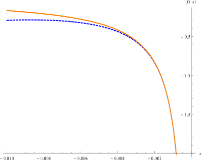
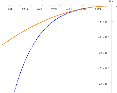
Figure 1: The left figure shows a plot of the first term of the integrand of Eq. (44) for fixed values $u=1,v=0.5,z=-0.01$, i.e. $f(x)\equiv y_{1}(x)F[0.5x,1x,-0.01]$ with $x\in[z,0]$. The right figure shows a plot of the second term of the integrand of Eq. (44) for fixed values $u=1,v=0.5,z=-0.01$, i.e. $f(x)\equiv j_{1}(x)F[0.5x,1x,-0.01]$ with $x\in[z,0]$ The blue-dashed curves represent the total functions, while the orange ones represent the first two non-null terms of the approximations.

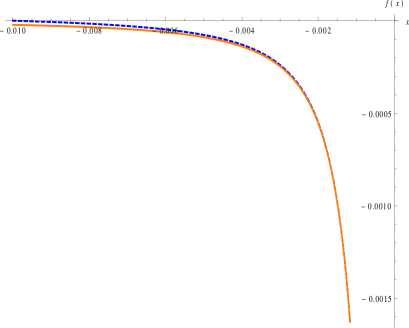
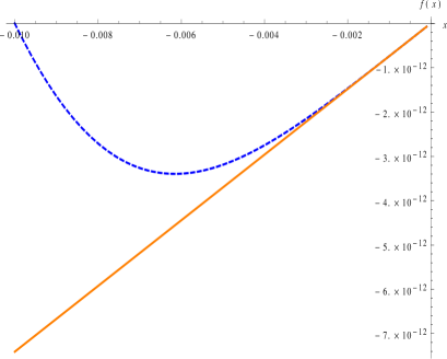
Figure 2: The left figure shows a plot of the first term of the integrand of Eq. (46) for fixed values $u=1,v=0.5,z=-0.01$, i.e. $f(x)\equiv y_{1}(x)F_{2}[0.5x,1x,-0.01]$ with $x\in[z,0]$. The right figure shows a plot of the second term of the integrand of Eq. (44) for fixed values $u=1,v=0.5,z=-0.01$, i.e. $f(x)\equiv j_{1}(x)F_{2}[0.5x,1x,-0.01]$ with $x\in[z,0]$ The blue-dashed curves represent the total functions, while the orange ones represent the first two non-null terms of the approximations.

Figures (1) and (2) show that the approximations used in both integrals $I_{1}(v,u,x,z)$ and $I_{2}(v,u,x,z)$ are viable when $x\to 0^{-}$ and $u$, $v$ and $z$ are fixed (we have found that for different values of $v$, $u$ and $z$, the graphics are not significantly modified). Moreover $I_{2}(v,u,x,z)\simeq 2I_{1}(v,u,x,z)$; consequently, substituting Eqs. (45) and (47) into Eq. (39) yields

$$P_{T}(k,\eta) \simeq x^{4}\frac{H^{4}}{8\pi^{4}M_{P}^{4}}\int_{0}^{\infty}dv\int_{|v-1|}^{|v+1|}du\frac{[4v^{2}-(u^{2}-v^{2}-1)^{2}]^{2}}{u^{2}v^{2}}$$

$$\times 2\bigg{[}\frac{R_{1}(z)^{2}}{3}\bigg{(}\frac{3}{2}-\frac{x}{z}-\frac{z^{2}}{2x^{2}}\bigg{)}+\frac{R_{1}(z)R_{2}(z)}{3}(v-u)z\bigg{(}\frac{x}{z}\ln\frac{z}{x}+\frac{x}{3z}-\frac{z^{2}}{3x^{2}}\bigg{)}\bigg{]}^{2},$$

We can rewrite the above expression in the following way

$$P_{T}(k,\eta) \simeq x^{4}\frac{H^{4}}{8\pi^{4}M_{P}^{4}}\frac{2}{9}\bigg{[}R_{1}(z)^{4}\bigg{(}\frac{3}{2}-\frac{x}{z}-\frac{z^{2}}{2x^{2}}\bigg{)}^{2}M_{1}+2R_{1}(z)^{3}R_{2}(z)z\bigg{(}\frac{3}{2}-\frac{x}{z}-\frac{z^{2}}{2x^{2}}\bigg{)}\bigg{(}\frac{x}{z}\ln\frac{z}{x}+\frac{x}{3z}-\frac{z^{2}}{3x^{2}}\bigg{)}M_{2}$$ (49)

$$+ R_{1}(z)^{2}R_{2}(z)^{2}z^{2}\bigg{(}\frac{x}{z}\ln\frac{z}{x}+\frac{x}{3z}-\frac{z^{2}}{3x^{2}}\bigg{)}^{2}M_{3}\bigg{]}$$

with $M_{1}$, $M_{2}$ and $M_{3}$ defined explicitly in Appendix A.

Furthermore, with the expressions for the tensor and scalar power spectra at hand, Eqs. (49) and (7) respectively, we can estimate the tensor-to-scalar ratio defined as $r\equiv P_{T}/P_{S}$, thus

$$r \simeq \frac{16x^{4}H^{2}\epsilon}{9\pi^{2}M_{P}^{2}}\bigg{[}R_{1}(z)^{2}\bigg{(}\frac{3}{2}-\frac{x}{z}-\frac{z^{2}}{2x^{2}}\bigg{)}^{2}M_{1}+2R_{1}(z)R_{2}(z)z\bigg{(}\frac{3}{2}-\frac{x}{z}-\frac{z^{2}}{2x^{2}}\bigg{)}\bigg{(}\frac{x}{z}\ln\frac{z}{x}+\frac{x}{3z}-\frac{z^{2}}{3x^{2}}\bigg{)}M_{2}$$ (50)

$$+ R_{2}(z)^{2}z^{2}\bigg{(}\frac{x}{z}\ln\frac{z}{x}+\frac{x}{3z}-\frac{z^{2}}{3x^{2}}\bigg{)}^{2}M_{3}\bigg{]}$$

Note that in expression above, we have made use of Eq. (7), with $n_{s}\simeq 1$, i.e. $P_{S}(k,\eta)\simeq H^{2}/(64\pi^{2}M_{P}^{2}\epsilon)R_{1}(z)^{2}$; also note that the function involving the time of collapse in the scalar power spectrum is exactly the same as $R_{1}(z)^{2}$.

Now we can use the fact that the observational data constrain the value of the scalar power spectrum to be $10^{-9}$. That is, in our approach, this constraint implies that $P_{S}(k,\eta)\simeq H^{2}/(64\pi^{2}M_{P}^{2}\epsilon)R_{1}(z)^{2}\simeq 10^{-9}$; thus,

$$\frac{H^{2}}{\pi^{2}M_{P}^{2}}\simeq\frac{10^{-9}8^{2}\epsilon}{R_{1}(z)^{2}}.$$ (51)

Equation (51) means that, in order to our approach to be consistent with the observations associated to the scalar power spectrum, the time of collapse must satisfy $H^{2}/(64\pi^{2}M_{P}^{2}\epsilon)R_{1}(z)^{2}\simeq 10^{-9}$.

Substituting Eq. (51) in Eq. (50) yields

$$r \simeq \frac{1024}{9}10^{-9}\epsilon^{2}x^{4}\bigg{[}\bigg{(}\frac{3}{2}-\frac{x}{z}-\frac{z^{2}}{2x^{2}}\bigg{)}^{2}M_{1}+2\frac{R_{2}(z)z}{R_{1}(z)}\bigg{(}\frac{3}{2}-\frac{x}{z}-\frac{z^{2}}{2x^{2}}\bigg{)}\bigg{(}\frac{x}{z}\ln\frac{z}{x}+\frac{x}{3z}-\frac{z^{2}}{3x^{2}}\bigg{)}M_{2}$$ (52)

$$+ \frac{R_{2}(z)^{2}z^{2}}{R_{1}(z)^{2}}\bigg{(}\frac{x}{z}\ln\frac{z}{x}+\frac{x}{3z}-\frac{z^{2}}{3x^{2}}\bigg{)}^{2}M_{3}\bigg{]}$$

Finally, since we have assumed that the time of collapse occurs when the proper wavelength of the mode is bigger than the Hubble radius, i.e. $|z|=-k\eta_{\vec{k}}^{c}<1$, then we can expand in series the functions $R_{2}(z)z/R_{1}(z)$ and $R_{2}(z)^{2}z^{2}/R_{1}(z)^{2}$ around $z=0$; additionally we will use that $|z|=-k\eta_{\vec{k}}^{c}>-k\eta=|x|$ with $x=k\eta\to 0^{-}$, and retain the leading terms in $x/z$. Thus, Eq. (52) is approximated by

$$r\simeq\frac{1024}{9}10^{-9}\epsilon^{2}\bigg{(}\frac{z^{4}}{4}M_{1}-z^{2}M_{2}+M_{3}\bigg{)}$$ (53)

Equation (53) is the first main result of this section. We can see that the prediction for $r$ given by the collapse hypothesis within the semiclassical gravity framework, is suppressed by a factor of $10^{-9}\epsilon^{2}$ and by powers of $|z|<1$. In other words, the generically predicted tensor-to-scalar ratio is extremely small making it practically undetectable by recent or future experiments. However, it is still within the observational bounds provided by the latest Planck results BICEP2/Keck and Planck Collaborations et al. (2015); Planck Collaboration et al. (2015), which set $r<0.12$. Moreover, Eq. (53) shows a degeneration between the slow roll parameter $\epsilon$ and the time of collapse. Therefore, if future experiments confirm a possible detection of primordial gravitational waves, in clear contrast to the standard approach, the measured value of $r$ would not fix the value of the slow-roll parameter $\epsilon$, it would only fix a combination of $\epsilon$ and the value of the time of collapse $z$. Consequently, the confirmed detection of primordial $B$-modes would make this whole scenario, i.e. the self-induced collapse hypothesis within the semiclassical gravity, extremely unlikely.

We will focus now on the second case, that is, the time of collapse occurs when the proper wavelength of the mode is smaller than the Hubble radius $z=k\eta_{\vec{k}}^{c}\to-\infty$ i.e. at the very beginning of the inflationary regime.

We begin this case with Eq. (42) which corresponds to the tensor power spectrum and proceed to calculate the tensor-to-scalar ratio $r\equiv P_{T}/P_{S}$ where $P_{S}(k,\eta)\simeq H^{2}/(64\pi^{2}M_{P}^{2}\epsilon)R_{1}(z)^{2}$, Eq. (7); additionally, by considering that the time of collapse must satisfy $H^{2}/(64\pi^{2}M_{P}^{2}\epsilon)R_{1}(z)^{2}\simeq 10^{-9}$, the prediction for $r$ is

$$r\simeq 8^{3}10^{-9}\epsilon^{2}\frac{x^{4}}{R_{1}(z)^{4}}\int_{0}^{\infty}dv\int_{|v-1|}^{|v+1|}du\frac{[4v^{2}-(u^{2}-v^{2}-1)^{2}]^{2}}{u^{2}v^{2}}I_{1}(v,u,x,z)I_{2}(v,u,x,z)$$ (54)

Next, we focus on the integrals $I_{1}(v,u,x,z),I_{2}(v,u,x,z)$. These integrals can be rewritten as

$$I_{1}(v,u,x,z)=\int_{-\infty}^{x}d\tilde{x_{1}}G(x,\tilde{x_{1}})[R_{1}(z)^{2}f_{1}(v\tilde{x_{1}},u\tilde{x_{1}})+R_{1}(z)R_{2}(z)f_{2}(v\tilde{x_{1}},u\tilde{x_{1}})+R_{2}(z)^{2}f_{3}(v\tilde{x_{1}},u\tilde{x_{1}})],$$ (55a)

$$I_{2}(v,u,x,z)=\int_{-\infty}^{x}d\tilde{x_{2}}G(x,\tilde{x_{2}})[R_{1}(z)^{2}\tilde{f}_{1}(v\tilde{x_{2}},u\tilde{x_{2}})+R_{1}(z)R_{2}(z)\tilde{f}_{2}(v\tilde{x_{2}},u\tilde{x_{2}})+R_{2}(z)^{2}\tilde{f}_{3}(v\tilde{x_{2}},u\tilde{x_{2}})],$$ (55b)

note that the lower limit of integration takes into account that we are considering the case $z\to-\infty$. The explicit forms of the functions $f_{1},f_{2},f_{3}$ and $\tilde{f}_{1},\tilde{f}_{2},\tilde{f}_{3}$ can be found in Appendix A. The advantage of writing the integrals $I_{1}(v,u,x,z),I_{2}(v,u,x,z)$ in the form of Eqs. (55) is that the dependence on the time of collapse is totally contained in the functions $R_{1}(z)$ and $R_{2}(z)$.

Substituting Eqs. (55) in Eq. (54) we have

$$r\simeq 10^{-9}\epsilon^{2}\bigg{[}C_{0}(x)+C_{1}(x)\frac{R_{2}(z)}{R_{1}(z)}+C_{2}(x)\bigg{(}\frac{R_{2}(z)}{R_{1}(z)}\bigg{)}^{2}+C_{3}(x)\bigg{(}\frac{R_{2}(z)}{R_{1}(z)}\bigg{)}^{3}+C_{4}(x)\bigg{(}\frac{R_{2}(z)}{R_{1}(z)}\bigg{)}^{4}\bigg{]},$$ (56)

note that $r$ written in this form exhibits explicitly the dependence on the time of collapse $z=k\eta_{\vec{k}}^{c}$. The explicit form of the functions $C_{0}(x),C_{1}(x),C_{2}(x),C_{3}(x),C_{4}(x)$ can be found in Appendix A; also, it should be noted that such functions should be evaluated at $x\to 0^{-}$ i.e. at a time near the end of inflation.

Next, using that $R_{2}(z)/R_{1}(z)=(\sin z+\cos z/z)/(\cos z-\sin z/z)$ and since we are interested in the case $z\to-\infty$, then we can approximate

$$\frac{R_{2}(z)}{R_{1}(z)}\simeq\tan(z)\equiv\zeta,$$ (57)

hence $-\infty<\zeta<\infty$. consequently Eq. (56) is given by

$$r\simeq 10^{-9}\epsilon^{2}\bigg{[}C_{0}(x)+C_{1}(x)\zeta+C_{2}(x)\zeta^{2}+C_{3}(x)\zeta^{3}+C_{4}(x)\zeta^{4}\bigg{]}\qquad\textrm{with}\qquad x\to 0^{-}.$$ (58)

Equation (58) is the second main result of this section. It shows the prediction for $r$ in the case when the time of collapse occurs near the beginning of the inflationary era. As in the previous case, the generic prediction for $r$, within our approach, is suppressed by a factor of $10^{-9}\epsilon^{2}$. Note also that, even if $\zeta$ is in the range $(-\infty,\infty)$, its value starts to grow only near $z=-n\pi/2$ [with $n$ a (large) odd number], that is, for a generic value of $z$, the function $\zeta=\tan(z)$ does not grows arbitrarily large. Therefore, the prediction for $r$ in this case is also consistent with recent observational data given that it is suppressed by the square of the slow-roll parameter.

As in the case when $|z|<1$, a hypothetical measurement of $r$ would translate into a bound on a combination of the slow-roll parameter $\epsilon$ and the time of collapse. Consequently, the same discussion about the plausibility of the collapse model in the case when the time of collapse satisfies $-k\eta_{\vec{k}}^{c}<1$ also applies in the present case, i.e. when the time of collapse is such that $k\eta_{\vec{k}}^{c}\to-\infty$.

To end this section, let us summarize the general conditions and motivations under which results (53) and (58) were achieved and their extension to specific inflationary models.

Our collapse proposal is meant to serve as a possible explanation to the generation of primordial perturbations, in particular the primordial gravitational waves. In a broad sense, we are considering the standard inflationary paradigm with the addition of the self-induced collapse hypothesis and the semiclassical gravity framework. In the present article, we have focused on the simplest inflationary model (and also the one favored by recent Planck data Planck Collaboration et al. (2015)), namely a single adiabatic Gaussian scalar field (the inflaton) minimally coupled to gravity with canonical kinetic term in the slow-roll approximation.

As regards with the characteristics of the self-induced collapse, the only assumption we have made is that the time of collapse $\eta_{\vec{k}}^{c}$ is proportional to $k^{-1}$; this relation was phenomenologically inferred from previous works by comparing the theoretical predictions (specifically the scalar angular power spectrum) with the observational data. Therefore, the relation $k\eta_{\vec{k}}^{c}$ implies a specific dependence of the time of collapse: $\eta_{\vec{k}}^{c}=z/k$, being $z$ a free parameter of the collapse model.

In fact, any inflationary model satisfying the previous conditions (with the inclusion of the self-induced collapse and the semiclassical Einstein equations) would yield a similar suppression for $r$ that is compatible with results (53) and (58). For example, Starobinsky’s inflationary model Starobinsky (1980); Mukhanov and Chibisov (1981); Starobinsky (1983) (also known as $R+R^{2}$ inflation) can be characterized by the action of a single-scalar field with canonical kinetic term, and a potential with a region in which the slow-roll approximation is valid; Starobinsky’s model predicts a value Kehagias et al. (2014) for the slow-roll parameter $|\epsilon|\simeq 3/(4N^{2})$, with $N$ the number of $e$-foldings characteristic of inflation; thus, for $N\simeq 60$, one has $|\epsilon|\simeq 10^{-4}$. This is, for the Starobinsky’s model, the value of $r$, within our approach, would be suppressed by a factor $10^{-9}\epsilon^{2}=10^{-17}$ Thus, the conclusions drawn from the results (53) and (58) apply to generic single-field slow-roll models within the semiclassical gravity framework and the self-induced collapse.

VII Summary and Conclusions

In this paper we have computed the tensor primordial power spectrum and the tensor-to-scalar ratio $r$ by making use of semiclassical Einstein equations and also including a self-induced collapse of the inflaton’s wave function. Within the semiclassical gravity approximation there is no source for tensor modes at the first-order perturbation theory; to calculate the tensor power spectrum the second-order has to be considered.

We have considered two cases: 1) the time of collapse occurs when the proper wavelength of the mode is greater than the Hubble radius, that is $-k\eta_{\vec{k}}^{c}<1$ and 2) the time of collapse occurs when the proper wavelength of the mode is smaller than the Hubble radius, that is $k\eta_{\vec{k}}^{c}\to-\infty$. In both cases a generic value for $z$ results in a prediction of $r$ that is suppressed by a factor of $10^{-9}\epsilon^{2}$, that is, a very small value; nevertheless, it is still consistent with the limit obtained by the joint analysis performed by the BICEP/KECK and PLANCK collaborations.

On the contrary, if a detection of primordial $B$ modes is confirmed, then the self-induced collapse hypothesis plus the semiclassical gravity approach would face severe issues given the degeneration between the slow roll parameter $\epsilon$ and the time of collapse in the prediction of $r$ [see Eqs. (53) and (58)].

However, we have also discussed in this paper, that the discrepancy with standard inflationary model prediction’s arises in considering the semiclassical approximation and not the self-induced collapse of the inflaton’s wave function. Within the semiclassical approximation, tensor modes are different from zero only at second-order perturbation theory, while in the standard procedure (where a joint quantization of the metric and field is performed) the tensor modes can be generated at first-order in the perturbation theory. Furthermore, a recent calculation of the tensor-to-scalar ratio using the Mukhanov-Sasaki variable and including the collapse of the wave function Mariani et al. (2014); Leon and Bengochea (2015) gives a prediction of the value of $r$ closest to the upper bound given by the joint BICEP/KECK and Planck collaboration’s analysis.

Appendix A Expressions used in Sec. VI

In this appendix we provide the explicit form of the expression used in Sec. VI.

The quantities $M_{1}$, $M_{2}$ and $M_{3}$ are defined as

$$M_{1}\equiv\int_{0}^{\infty}dv\int_{|v-1|}^{|v+1|}du\frac{[4v^{2}-(u^{2}-v^{2}-1)^{2}]^{2}}{u^{2}v^{2}},$$ (59a)

$$M_{2}\equiv\int_{0}^{\infty}dv\int_{|v-1|}^{|v+1|}du\frac{[4v^{2}-(u^{2}-v^{2}-1)^{2}]^{2}}{u^{2}v^{2}}(v-u),$$ (59b)

$$M_{3}\equiv\int_{0}^{\infty}dv\int_{|v-1|}^{|v+1|}du\frac{[4v^{2}-(u^{2}-v^{2}-1)^{2}]^{2}}{u^{2}v^{2}}(v-u)^{2}.$$ (59c)

The functions $f_{1}(v\tilde{x_{1}},u\tilde{x_{1}})$, $f_{2}(v\tilde{x_{1}},u\tilde{x_{1}})$ and $f_{3}(v\tilde{x_{1}},u\tilde{x_{1}})$ used in Eqs. (55) are defined as

$$f_{1}(v\tilde{x_{1}},u\tilde{x_{1}})\equiv\cos(u\tilde{x_{1}})\cos(v\tilde{x_{1}})+uv\tilde{x_{1}}^{2}\sin(u\tilde{x_{1}})\sin(v\tilde{x_{1}})+2u\tilde{x_{1}}\cos(v\tilde{x_{1}})\sin(u\tilde{x_{1}}),$$ (60a)

$$f_{2}(v\tilde{x_{1}},u\tilde{x_{1}})\equiv-2u\tilde{x_{1}}\cos[(u+v)\tilde{x_{1}}]+(1-uv\tilde{x_{1}}^{2})\sin[(u+v)\tilde{x_{1}}],$$ (60b)

$$f_{3}(v\tilde{x_{1}},u\tilde{x_{1}})\equiv uv\tilde{x_{1}}^{2}\cos(u\tilde{x_{1}})\cos(v\tilde{x_{1}})+\sin(u\tilde{x_{1}})\sin(v\tilde{x_{1}})-2u\tilde{x_{1}}\sin(v\tilde{x_{1}})\cos(u\tilde{x_{1}}).$$ (60c)

Meanwhile, the functions $\tilde{f}_{1}(v\tilde{x_{1}},u\tilde{x_{1}})$, $\tilde{f}_{2}(v\tilde{x_{1}},u\tilde{x_{1}})$ and $\tilde{f}_{3}(v\tilde{x_{1}},u\tilde{x_{1}})$ also used in Eqs. (55) are defined as

$$\tilde{f}_{1}(v\tilde{x_{2}},u\tilde{x_{2}})\equiv 2[\cos(u\tilde{x_{2}})\cos(v\tilde{x_{2}})+uv\tilde{x_{2}}^{2}\sin(u\tilde{x_{2}})\sin(v\tilde{x_{2}})+2u\tilde{x_{2}}\cos(v\tilde{x_{2}})\sin(u\tilde{x_{2}})+2v\tilde{x_{2}}\cos(u\tilde{x_{2}})\sin(v\tilde{x_{2}})],$$ (61a)

$$\tilde{f}_{2}(v\tilde{x_{2}},u\tilde{x_{2}})\equiv(-2u\tilde{x_{2}}-2v\tilde{x_{2}})\cos[(u+v)\tilde{x_{2}}]+2(1-uv\tilde{x_{2}}^{2})\sin[(u+v)\tilde{x_{2}}],$$ (61b)

$$\tilde{f}_{3}(v\tilde{x_{2}},u\tilde{x_{2}})\equiv 2[uv\tilde{x_{2}}^{2}\cos(u\tilde{x_{2}})\cos(v\tilde{x_{2}})+\sin(u\tilde{x_{2}})\sin(v\tilde{x_{2}})-u\tilde{x_{2}}\sin(v\tilde{x_{2}})\cos(u\tilde{x_{2}})-v\tilde{x_{2}}\cos(v\tilde{x_{2}}).\sin(u\tilde{x_{2}})]$$ (61c)

The functions $C_{0}(x)$, $C_{1}(x)$, $C_{2}(x)$, $C_{3}(x)$ and $C_{4}(x)$ used in Eqs. (56) and (58) are defined as

$$C_{0}(x) \equiv 8^{3}x^{4}\int_{0}^{\infty}dv\int_{|v-1|}^{|v+1|}du\int_{-\infty}^{x}d\tilde{x_{1}}\int_{-\infty}^{x}d\tilde{x_{2}}\>G(x,\tilde{x}_{1})G(x,\tilde{x}_{2})\frac{[4v^{2}-(u^{2}-v^{2}-1)^{2}]^{2}}{u^{2}v^{2}}$$ (62a)

$$\times f_{1}(v\tilde{x_{1}},u\tilde{x_{1}})\tilde{f}_{1}(v\tilde{x_{2}},u\tilde{x_{2}}),$$

$$C_{1}(x) \equiv 8^{3}x^{4}\int_{0}^{\infty}dv\int_{|v-1|}^{|v+1|}du\int_{-\infty}^{x}d\tilde{x_{1}}\int_{-\infty}^{x}d\tilde{x_{2}}\>G(x,\tilde{x}_{1})G(x,\tilde{x}_{2})\frac{[4v^{2}-(u^{2}-v^{2}-1)^{2}]^{2}}{u^{2}v^{2}}$$ (62b)

$$\times [f_{2}(v\tilde{x_{1}},u\tilde{x_{1}})\tilde{f}_{1}(v\tilde{x_{2}},u\tilde{x_{2}})+f_{1}(v\tilde{x_{1}},u\tilde{x_{1}})\tilde{f}_{2}(v\tilde{x_{2}},u\tilde{x_{2}})],$$

$$C_{2}(x) \equiv 8^{3}x^{4}\int_{0}^{\infty}dv\int_{|v-1|}^{|v+1|}du\int_{-\infty}^{x}d\tilde{x_{1}}\int_{-\infty}^{x}d\tilde{x_{2}}\>G(x,\tilde{x}_{1})G(x,\tilde{x}_{2})\frac{[4v^{2}-(u^{2}-v^{2}-1)^{2}]^{2}}{u^{2}v^{2}}$$ (62c)

$$\times [f_{3}(v\tilde{x_{1}},u\tilde{x_{1}})\tilde{f}_{1}(v\tilde{x_{2}},u\tilde{x_{2}})+f_{1}(v\tilde{x_{1}},u\tilde{x_{1}})\tilde{f}_{3}(v\tilde{x_{2}},u\tilde{x_{2}})+f_{2}(v\tilde{x_{1}},u\tilde{x_{1}})\tilde{f}_{2}(v\tilde{x_{2}},u\tilde{x_{2}})],$$

$$C_{3}(x) \equiv 8^{3}x^{4}\int_{0}^{\infty}dv\int_{|v-1|}^{|v+1|}du\int_{-\infty}^{x}d\tilde{x_{1}}\int_{-\infty}^{x}d\tilde{x_{2}}\>G(x,\tilde{x}_{1})G(x,\tilde{x}_{2})\frac{[4v^{2}-(u^{2}-v^{2}-1)^{2}]^{2}}{u^{2}v^{2}}$$ (62d)

$$\times [f_{3}(v\tilde{x_{1}},u\tilde{x_{1}})\tilde{f}_{2}(v\tilde{x_{2}},u\tilde{x_{2}})+f_{2}(v\tilde{x_{1}},u\tilde{x_{1}})\tilde{f}_{3}(v\tilde{x_{2}},u\tilde{x_{2}})],$$

$$C_{4}(x) \equiv 8^{3}x^{4}\int_{0}^{\infty}dv\int_{|v-1|}^{|v+1|}du\int_{-\infty}^{x}d\tilde{x_{1}}\int_{-\infty}^{x}d\tilde{x_{2}}\>G(x,\tilde{x}_{1})G(x,\tilde{x}_{2})\frac{[4v^{2}-(u^{2}-v^{2}-1)^{2}]^{2}}{u^{2}v^{2}}$$ (62e)

$$\times f_{3}(v\tilde{x_{1}},u\tilde{x_{1}})\tilde{f}_{3}(v\tilde{x_{2}},u\tilde{x_{2}}).$$

References

- Martin et al. (2014a) J. Martin, C. Ringeval, R. Trotta, and V. Vennin, Journal of Cosmology and Astroparticle Physics 3, 039 (2014a), eprint 1312.3529.
- Martin et al. (2014b) J. Martin, C. Ringeval, and V. Vennin, Physics of the Dark Universe 5, 75 (2014b), eprint 1303.3787.
- The Polarbear Collaboration: P. A. R. Ade et al. (2014) The Polarbear Collaboration: P. A. R. Ade, Y. Akiba, A. E. Anthony, K. Arnold, M. Atlas, D. Barron, D. Boettger, J. Borrill, S. Chapman, Y. Chinone, et al., Astrophys. J. 794, 171 (2014), eprint 1403.2369.
- Ade et al. (2014) P. A. R. Ade, R. W. Aikin, D. Barkats, S. J. Benton, C. A. Bischoff, J. J. Bock, J. A. Brevik, I. Buder, E. Bullock, C. D. Dowell, et al., Physical Review Letters 112, 241101 (2014), eprint 1403.3985.
- Mortonson and Seljak (2014) M. J. Mortonson and U. Seljak, Journal of Cosmology and Astroparticle Physics 10, 035 (2014), eprint 1405.5857.
- Flauger et al. (2014) R. Flauger, J. C. Hill, and D. N. Spergel, JCAP 1408, 039 (2014), eprint 1405.7351.
- Liu et al. (2014) H. Liu, P. Mertsch, and S. Sarkar, Astrophysical Journal Letters 789, L29 (2014), eprint 1404.1899.
- Planck Collaboration et al. (2014) Planck Collaboration, R. Adam, P. A. R. Ade, N. Aghanim, M. Arnaud, J. Aumont, C. Baccigalupi, A. J. Banday, R. B. Barreiro, J. G. Bartlett, et al., ArXiv e-prints (2014), eprint 1409.5738.
- BICEP2/Keck and Planck Collaborations et al. (2015) BICEP2/Keck and Planck Collaborations, P. A. R. Ade, N. Aghanim, Z. Ahmed, R. W. Aikin, K. D. Alexander, M. Arnaud, J. Aumont, C. Baccigalupi, A. J. Banday, et al., Physical Review Letters 114, 101301 (2015), eprint 1502.00612.
- Landau et al. (2013) S. J. Landau, G. León, and D. Sudarsky, Physical Review D 88, 023526 (2013), eprint 1107.3054.
- Perez et al. (2006) A. Perez, H. Sahlmann, and D. Sudarsky, Class. Quant. Grav. 23, 2317 (2006), eprint gr-qc/0508100.
- Sudarsky (2011) D. Sudarsky, International Journal of Modern Physics D 20, 509 (2011), eprint 0906.0315.
- Sudarsky (2007) D. Sudarsky, J. Phys. Conf. Ser. 68, 012029 (2007), eprint gr-qc/0612005.
- de Unánue and Sudarsky (2008) A. de Unánue and D. Sudarsky, Physical Review D 78, 043510 (2008), eprint arXiv:0801.4702.
- León and Sudarsky (2010) G. León and D. Sudarsky, Classical and Quantum Gravity 27, 225017 (2010), eprint 1003.5950.
- León et al. (2011) G. León, A. De Unánue, and D. Sudarsky, Classical and Quantum Gravity 28, 155010 (2011), eprint 1012.2419.
- Diez-Tejedor and Sudarsky (2012) A. Diez-Tejedor and D. Sudarsky, JCAP 7, 045 (2012), eprint 1108.4928.
- Landau et al. (2012) S. J. Landau, C. G. Scóccola, and D. Sudarsky, Physical Review D 85, 123001 (2012), eprint 1112.1830.
- Cañate et al. (2013) P. Cañate, P. Pearle, and D. Sudarsky, Phys.Rev. D 87, 104024 (2013), eprint 1211.3463.
- León et al. (2014) G. León, S. J. Landau, and M. P. Piccirilli, Phys. Rev. D90, 083525 (2014), eprint 1410.1562.
- León and Sudarsky (2015) G. León and D. Sudarsky, JCAP 1506, 020 (2015), eprint 1503.01417.
- Markkanen et al. (2015) T. Markkanen, S. Rasanen, and P. Wahlman, Phys. Rev. D91, 084064 (2015), eprint 1407.4691.
- Diez-Tejedor et al. (2012) A. Diez-Tejedor, G. Leon, and D. Sudarsky, Gen.Rel.Grav. 44, 2965 (2012), eprint 1106.1176.
- DeWitt (1967) B. S. DeWitt, Phys.Rev. 160, 1113 (1967).
- Giulini and Kiefer (2007) D. Giulini and C. Kiefer, Lect.Notes Phys. 721, 131 (2007), eprint gr-qc/0611141.
- Isham (1992) C. Isham, Canonical quantum gravity and the problem of time (1992), eprint gr-qc/9210011.
- Okon and Sudarsky (2015) E. Okon and D. Sudarsky, Found.Phys. 45, 461 (2015), eprint 1406.2011.
- Modak et al. (2015a) S. K. Modak, L. Ortíz, I. Peña, and D. Sudarsky, Gen. Rel. Grav. 47, 120 (2015a), eprint 1406.4898.
- Modak et al. (2015b) S. K. Modak, L. Ortíz, I. Peña, and D. Sudarsky, Phys. Rev. D91, 124009 (2015b), eprint 1408.3062.
- Jacobson and Hu (1993) T. Jacobson and B. L. Hu, Directions in General Reltivity (Cambridge University Press (UK), 1993).
- Ashtekar (2013) A. Ashtekar, Quantum geometry and gravity: Recent advances (2013), eprint gr-qc/0112038.
- Mariani et al. (2014) M. Mariani, G. R. Bengochea, and G. Leon, Inflationary gravitational waves in collapse scheme models (2014), eprint 1412.6471.
- Leon and Bengochea (2015) G. Leon and G. R. Bengochea, Emergence of inflationary perturbations in the CSL model (2015), eprint 1502.04907.
- Bassi and Ghirardi (2003) A. Bassi and G. C. Ghirardi, Phys.Rept. 379, 257 (2003), eprint quant-ph/0302164.
- Penrose (1996) R. Penrose, Gen.Rel.Grav. 28, 581 (1996).
- Diosi (1987) L. Diosi, Phys.Lett. A120, 377 (1987).
- Mollerach and Matarrese (1997) S. Mollerach and S. Matarrese, Phys.Rev. D56, 4494 (1997), eprint astro-ph/9702234.
- Mollerach (1998) S. Mollerach, Phys.Rev. D57, 1303 (1998), eprint astro-ph/9708196.
- Mollerach et al. (2004) S. Mollerach, D. Harari, and S. Matarrese, Phys.Rev. D69, 063002 (2004), eprint astro-ph/0310711.
- Osano et al. (2007) B. Osano, C. Pitrou, P. Dunsby, J.-P. Uzan, and C. Clarkson, JCAP 0704, 003 (2007), eprint gr-qc/0612108.
- Ananda et al. (2007) K. N. Ananda, C. Clarkson, and D. Wands, Phys.Rev. D75, 123518 (2007), eprint gr-qc/0612013.
- Baumann et al. (2007) D. Baumann, P. J. Steinhardt, K. Takahashi, and K. Ichiki, Phys.Rev. D76, 084019 (2007), eprint hep-th/0703290.
- León et al. (2015) G. León, S. J. Landau, and M. P. Piccirilli, Eur. Phys. J. C75, 393 (2015), eprint 1502.00921.
- Acquaviva et al. (2003) V. Acquaviva, N. Bartolo, S. Matarrese, and A. Riotto, Nucl.Phys. B667, 119 (2003), eprint astro-ph/0209156.
- Planck Collaboration et al. (2015) Planck Collaboration, P. A. R. Ade, N. Aghanim, M. Arnaud, F. Arroja, M. Ashdown, J. Aumont, C. Baccigalupi, M. Ballardini, A. J. Banday, et al., ArXiv e-prints (2015), eprint 1502.02114.
- Starobinsky (1980) A. A. Starobinsky, Phys.Lett. B91, 99 (1980).
- Mukhanov and Chibisov (1981) V. F. Mukhanov and G. V. Chibisov, JETP Lett. 33, 532 (1981).
- Starobinsky (1983) A. A. Starobinsky, Sov.Astron.Lett. 9, 302 (1983).
- Kehagias et al. (2014) A. Kehagias, A. M. Dizgah, and A. Riotto, Phys.Rev. D89, 043527 (2014), eprint 1312.1155.