An efficient algorithm for numerical computations of continuous densities of states
Abstract
In Wang-Landau type algorithms, Monte-Carlo updates are performed with respect to the density of states, which is iteratively refined during simulations. The partition function and thermodynamic observables are then obtained by standard integration. In this work, our recently introduced method in this class (the LLR approach) is analysed and further developed. Our approach is a histogram free method particularly suited for systems with continuous degrees of freedom giving rise to a continuum density of states, as it is commonly found in Lattice Gauge Theories and in some Statistical Mechanics systems. We show that the method possesses an exponential error suppression that allows us to estimate the density of states over several orders of magnitude with nearly-constant relative precision. We explain how ergodicity issues can be avoided and how expectation values of arbitrary observables can be obtained within this framework. We then demonstrate the method using Compact U(1) Lattice Gauge Theory as a show case. A thorough study of the algorithm parameter dependence of the results is performed and compared with the analytically expected behaviour. We obtain high precision values for the critical coupling for the phase transition and for the peak value of the specific heat for lattice sizes ranging from to . Our results perfectly agree with the reference values reported in the literature, which covers lattice sizes up to . Robust results for the volume are obtained for the first time. This latter investigation, which, due to strong metastabilities developed at the pseudo-critical coupling of the system, so far has been out of reach even on supercomputers with importance sampling approaches, has been performed to high accuracy with modest computational resources. This shows the potential of the method for studies of first order phase transitions. Other situations where the method is expected to be superior to importance sampling techniques are pointed out.
1 Introduction and motivations
Monte-Carlo methods are widely used in Theoretical Physics, Statistical Mechanics and Condensed Matter (for an overview, see e.g. landau2014guide ). Since the inception of the field metropolis , most of the applications have relied on importance sampling, which allows us to evaluate stochastically with a controllable error multi-dimensional integrals of localised functions. These methods have immediate applications when one needs to compute thermodynamic properties, since statistical averages of (most) observables can be computed efficiently with importance sampling techniques. Similarly, in Lattice Gauge Theories, most quantities of interest can be expressed in the path integral formalism as ensemble averages over a positive-definite (and sharply peaked) measure, which, once again, provide an ideal scenario for applying importance sampling methods.
However, there are noticeable cases in which Monte-Carlo importance sampling methods are either very inefficient or produce inherently wrong results for well understood reasons. Among those cases, some of the most relevant situations include systems with a sign problem (see Aarts:2015kea for a recent review), direct computations of free energies (comprising the study of properties of interfaces), systems with strong metastabilities (for instance, a system with a first order phase transition in the region in which the phases coexist) and systems with a rough free energy landscape. Alternatives to importance sampling techniques do exist, but generally they are less efficient in standard cases and hence their use is limited to ad-hoc situations in which more standard methods are inapplicable. Noticeable exceptions are micro-canonical methods, which have experienced a surge in interest in the past fifteen years. Most of the growing popularity of those methods is due to the work of Wang and Landau Wang:2001ab , which provided an efficient algorithm to access the density of states in a statistical system with a discrete spectrum. Once the density of states is known, the partition function (and from it all thermodynamic properties of the system) can be reconstructed by performing one-dimensional numerical integrals. The generalisation of the Wang-Landau algorithm to systems with a continuum spectrum is far from straightforward Xu:2007aa ; Sinha:2007aa . To overcome this limitation, a very promising method, here referred to as the Logarithmic Linear Relaxation (LLR) algorithm, was introduced in Langfeld:2012ah . The potentialities of the method were demonstrated in subsequent studies of systems afflicted by a sign problem Langfeld:2014nta ; Gattringer:2015lra , in the computation of the Polyakov loop probability distribution function in two-colour QCD with heavy quarks at finite density Langfeld:2013xbf and – rather unexpectedly – even in the determination of thermodynamic properties of systems with a discrete energy spectrum Guagnelli:2012dk .
The main purpose of this work is to discuss in detail some improvements of the original LLR algorithm and to formally prove that expectation values of observables computed with this method converge to the correct result, which fills a gap in the current literature. In addition, we apply the algorithm to the study of Compact U(1) Lattice Gauge Theory, a system with severe metastabilities at its first order phase transition point that make the determination of observables near the transition very difficult from a numerical point of view. We find that in the LLR approach correlation times near criticality grow at most quadratically with the volume, as opposed to the exponential growth that one expects with importance sampling methods. This investigation shows the efficiency of the LLR method when dealing with systems having a first order phase transition. These results suggest that the LLR method can be efficient at overcoming numerical metastabilities in other classes of systems with a multi-peaked probability distribution, such as those with rough free energy landscapes (as commonly found, for instance, in models of protein folding or spin glasses).
The rest of the paper is organised as follows. In Sect. 2 we cover the formal general aspects of the algorithm. The investigation of Compact U(1) Lattice Gauge Theory is reported in Sect. 3. A critical analysis of our findings, our conclusions and our future plans are presented in Sect. 4. Finally, some technical material is discussed in the appendix. Some preliminary results of this study have already been presented in Pellegrini:2014gha .
2 Numerical determination of the density of states
2.1 The density of states
Owing to formal similarities between the two fields, the approach we are proposing can be applied to both Statistical Mechanics and Lattice Field Theory systems. In order to keep the discussion as general as possible, we shall introduce notations and conventions that can describe simultaneously both cases. We shall consider a system described by the set of dynamical variables , which could represent a set of spin or field variables and are assumed to be continuous. The action (in the field theory case) or the Hamiltonian (for the statistical system) is indicated by and the coupling (or inverse temperature) by . Since the product is dimensionless, without loss of generality we will take both and dimensionless.
We consider a system with a finite volume , which will be sent to infinity in the final step of our calculations. The finiteness of in the intermediate steps allows us to define naturally a measure over the variables , which we shall call . Properties of the system can be derived from the function
which defines the canonical partition function for the statistical system or the path integral in the field theory case. The density of state (which is a function of the value of ) is formally defined by the integral
| (1) |
In terms of , takes the form
The vacuum expectation value (or ensemble average) of an observable which is function of can be written as111The most general case in which can not be written as a function of is discussed in Subsect. 2.3.
| (2) |
Hence, a numerical determination of would enable us to express and as numerical integrals of known functions in the single variable . This approach is inherently different from conventional Monte-Carlo calculations, which relie on the concept of importance sampling, i.e. the configurations contributing to the integral are generated with probability
Owing to this conceptual difference, the method we are proposing can overcome notorious drawbacks of importance sampling techniques.
2.2 The LLR method
We will now detail our approach to the evaluation of the density of states by means of a lattice simulations. Our initial assumption is that the density of states is a regular function of the energy that can be always approximated in a finite interval by a suitable functional expansion. If we consider the energy interval , under the physically motivated assumption that the density of states is a smooth function in this interval, the logarithm of the latter quantity can be written, using Taylor’s theorem, as
| (3) | |||||
Thereby, for a given action , the integer is chosen such that
Our goal will be to devise a numerical method to calculate the Taylor coefficients
| (4) |
and to reconstruct from these an approximation for the density of states . By introducing the intrinsic thermodynamic quantities, (temperature) and (specific heat) by
| (5) |
we expose the important feature that the target coefficients are independent of the volume while the correction is of order . In all practical applications, will be numerically much smaller than . For a certain parameter range (i.e., for the correlation length smaller than the lattice size), we can analytically derive this particular volume dependence of the density derivatives. Details are left to the appendix.
Using the trapezium rule for integration, we find in particular
| (6) |
Using this equation recursively, we find
| (7) |
Note that . Exponentiating (3) and using (7), we obtain
| (8) | |||||
| (9) |
where we have defined an overall multiplicative constant by
We are now in the position to introduce the piecewise-linear and continuous approximation of the density of states by
| (10) |
i.e., is chosen in such a way that for a given . With this definition, we obtain the remarkable identity
| (11) |
which we will extensively use below. We will observe that spans many orders of magnitude. The key observation is that our approximation implements exponential error suppression, meaning that can be approximated with nearly-constant relative error despite it may reach over thousands of orders of magnitude:
| (12) |
We will now present our method to calculate the coefficients . To this aim, we introduce the action restricted and re-weighted expectation values Langfeld:2012ah with being an external variable:
| (13) | |||||
| (14) |
where we have used (1) to express as an ordinary integral. We also introduced the modified Heaviside function
If the observable only depends on the action, i.e., , (13) simplifies to
| (15) |
Let us now consider the specific action observable
| (16) |
and the solution of the non-linear equation
| (17) |
Inserting from (8) into (15) and defining , we obtain:
| (18) | |||||
Let us consider for the moment the function
It is easy to check that is monotonic and vanishing for :
We therefore conclude for any that if (18) does have a solution, this solution is unique. For sufficiently small there is a solution, and, hence, the only solution is given by:
| (19) |
The later equation is at the heart of the LLR algorithm: it details how we can obtain the log-rho derivative by calculating the Monte-Carlo average (using (13)) and solving a non-linear equation, i.e., (17).
In the following, we will discuss the practical implementation by addressing two questions: (i) How do we solve the non-linear equation? (ii) How do we deal with the statistical uncertainty since the Monte-Carlo method only provides stochastic estimates for the expectation value ?
Let us start with the standard Newton-Raphson method to answer question (i). Starting from an initial guess for the solution, this method produces a sequence
which converges to the true solution . Starting from for the solution, we would like to derive an equation that generates a value that is even closer to the true solution:
| (20) |
Using the definition of in (18) with reference to (16) and (15), we find:
| (21) |
We thus find for the improved solution:
| (22) |
We can convert the Newton-Raphson recursion into a simpler fixed point iteration if we assume that the choice is sufficiently close to the true value such that
Without affecting the precision with which the solution of (18) can be obtained, we replace
| (23) |
Hence, the Newton-Raphson iteration is given by
| (24) |
We point out that one fixed point of the above iteration, i.e., , is attained for
which, indeed, is the correct solution. We have already shown that the above equation has only one solution. Hence, if the iteration converges at all, it necessarily converges to the true solution. Note that convergence can always be achieved by suitable choice of under-relaxation. We here point out that the solution to question (ii) above will involve a particular type of under-relaxation.
Let us address the question (ii) now. We have already pointed out that we have only a stochastic estimate for the expectation value and the convergence of the Newton-Raphson method is necessarily hampered by the inevitable statistical error of the estimator. This problem, however, has been already solved by Robbins and Monroe robbins1951 .
For completeness, we shall now give a brief presentation of the algorithm. The starting point is the function , and a constant , such that the equation has a unique root at . is only available by stochastic estimation using the random variable :
with being the ensemble average of . The iterative root finding problem is of the type
| (25) |
where is a sequence of positive numbers sizes satisfying the requirements
| (26) |
It is possible to prove that under certain assumptions robbins1951 on the function the converges in and hence in probability to the true value . A major advance in understanding the asymptotic properties of this algorithm was the main result of robbins1951 . If we restrict ourselves to the case
| (27) |
one can prove that is asymptotically normal with variance
| (28) |
where is the variance of the noise. Hence, the optimal value of the constant , which minimises the variance is given by
| (29) |
Adapting the Robbins-Monro approach to our root finding iteration in (24), we finally obtain an under-relaxed Newton-Raphson iteration
| (30) |
which is optimal with respect to the statistical noise during iteration.
2.3 Observables and convergence with
We have already pointed out that expectation values of observables depending on the action only can be obtained by a simple integral over the density of states (see (2)). Here we develop a prescription for determining the values of expectations of more general observables by folding with the numerical density of states and analyse the dependence of the estimate on .
Let us denote a generic observable by . Its expectation value is defined by
| (31) |
In order to relate to the LLR approach, we break up the latter integration into energy intervals:
| (32) |
Note that does not depend on .
We can express in terms of a sum over double-bracket expectation values by choosing
in (13). Without any approximation, we find:
| (33) | |||||
| (34) |
where is defined in (14). The above result can be further simplified by using (11):
| (35) | |||||
We now define the approximation to by
| (36) | |||||
| (37) |
Since the double-bracket expectation values do not produce a singularity if , i.e.,
using (35), from (33) and (34) we find that
| (38) |
The latter formula together with (36) provides access to all types of observables using the LLR method with little more computational resources: Once the Robbins-Monro iteration (30) has settled for an estimate of the coefficient , the Monte-Carlo simulation simply continues to derive estimators for the double-bracket expectation values in (36) and (37).
With the further assumption that the double-bracket expectation values are (semi-)positive, an even better error estimate is produced by our approach:
This implies that the observable can be calculated with an relative error of order . Indeed, we find from (33,34,35) that
| (40) |
Thereby, we have used
The assumption of (semi-)positive double expectation values is true for many action observables, and possibly also for Wilson loops, whose re-weighted and action restricted double expectation values might turn out to be positive (as it is the case for their standard expectation values). In this case, our method would provide an efficient determination of those quantities. This is important in particular for large Wilson loop expectation values, since they are notoriously difficult to measure with importance sampling methods (see e.g. Luscher:2001up ). We also note that, in order to have an accurate determination of a generic observable, any Monte-Carlo estimate of the double expectation values must be obtained to good precision dictated by the size of . A detailed numerical investigation of these and related issues is left to future work.
For the specific case that the observable only depends on the action , we circumvent this problem and evaluate the double-expectation values exactly. To this aim, we introduce for the general case the generalised density by
| (41) |
We then point out that if is depending on the action only, i.e., , we obtain:
With the definition of the double expectation value (13), we find:
| (42) |
Rather than calculating by Monte-Carlo methods, we can analytically evaluate this quantity (up to order ). Using the observation that for any smooth () function
and using this equation for both, numerator and denominator of (42), we conclude that
| (43) |
Let us now specialise to the case that is relevant for (2.3) with depending on the action only:
| (44) |
This leaves us with
| (45) |
Inserting (43) together with (44) into (36), we find:
| (46) | |||||
| (47) |
Below, we will numerically test the quality of expectation values obtained by the LLR approach using action observables only, i.e., . We will find that we indeed achieve the predicted precision in for this type of observables (see below Fig. 6).
2.4 The numerical algorithm
So far, we have shown that a piecewise continuous approximation of the density of states that is linear in intervals of sufficiently small amplitude allows us to obtain a controlled estimate of averages of observables and that the angular coefficients of the linear approximations can be computed in each interval using the Robbins-Monro recursion (30). Imposing the continuity of , one can then determine the latter quantity up to an additive constant, which does not play any role in cases in which observables are standard ensemble averages.
The Robbins-Monro recursion can be easily implemented in a numerical algorithm. Ideally, the recurrence would be stopped when a tolerance for is reached, i.e. when
| (48) |
with (for instance) set to the precision of the computation. When this condition is fulfilled, we can set . However, one has to keep into account the fact that the computation of requires an averaging over Monte-Carlo configurations. This brings into play considerations about thermalisation (which has to be taken into account each time we send ), the number of measurements used for determining at fixed and – last but not least – fluctuations of the themselves.
Following those considerations, an algorithm based on the Robbins-Monro recursion relation should depend on the following input (tunable) parameters:
-
•
, the number of Monte-Carlo updates in the restricted energy interval before starting to measure expectation values;
-
•
, the number of iterations used for computing expectation values;
-
•
, the number of Robbins-Monro iterations for determining ;
-
•
, number of final values from the Robbins-Monro iteration subjected to a subsequent bootstrap analysis.
The version of the LLR method proposed and implemented in this paper is reported in an algorithmic fashion in the box Algorithm 1. This implementation differs from that provided in Langfeld:2012ah ; Langfeld:2014nta by the replacement of the originally proposed root-finding procedure based on a deterministic Newton-Raphson like recursion with the Robbins-Monro recursion, which is better suited to the problem of finding zeros of stochastic equations.
Since the are determined stochastically, a different reiteration of the algorithm with different starting conditions and different random seeds would produce a different value for the same . The stochastic nature of the process implies that the distribution of the found in different runs is Gaussian. The generated ensemble of the can then be used to determine the error of the estimate of observables using analysis techniques such as jackknife and bootstrap.
The parameters and depend on the system and on the phenomenon under investigation. In particular, standard thermodynamic considerations on the infinite volume limit imply that if one is interested in a specific range of temperatures and the studied observables can be written as statistical averages with Gaussian fluctuations, it is possible to restrict the range of energies between the energy that is typical of the smallest considered temperature and the energy that is typical of the highest considered temperature. Determining a reasonable value for the amplitude of the energy interval and the other tunable parameters , , and requires a modest amount of experimenting with trial values. In our applications we found that the results were very stable for wide ranges of values of those parameters. Likewise, , the initial value for the Robbins-Monro recursion in interval , does not play a crucial role; when required and possible, an initial value close to the expected result can be inferred inverting , which can be obtained with a quick study using conventional techniques.
The average imposes an update that restricts configurations to those with energies in a specific range. In most of our studies, we have imposed the constraint analytically at the level of the generation of the newly proposed variables, which results in a performance that is comparable with that of the unconstrained system. Using a simple-minded more direct approach, in which one imposes the constraint after the generation of the proposed new variable, we found that in most cases the efficiency of Monte-Carlo algorithms did not drop drastically as a consequence of the restriction, and even for systems like SU(3) (see Ref. Langfeld:2012ah ) we were able to keep an efficiency of at least 30% and in most cases no less than 50% with respect to the unconstrained system.
2.5 Ergodicity
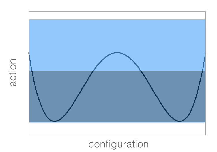
Our implementation of the energy restricted average assumes that the update algorithm is able to generate all configurations with energy in the relevant interval starting from configurations that have energy in the same interval. This assumption might be too strong when the update is local222This is for instance the case for the popular heath-bath and Metropolis update schemes. in the energy (i.e. each elementary update step changes the energy by a quantity of order one for a system with total energy of order ) and there are topological excitations that can create regions with the same energy that are separated by high energy barriers. In these cases, which are rather common in gauge theories and statistical mechanics333For instance, in a -dimensional Ising system of size , to go from one groundstate to the other one needs to create a kink, which has energy growing as ., generally in order to go from one acceptable region to the other one has to travel through a region of energies that is forbidden by an energy-restricted update method such as the LLR. Hence, by construction, in such a scenario our algorithm will get trapped in one of the allowed regions. Therefore, the update will not be ergodic.
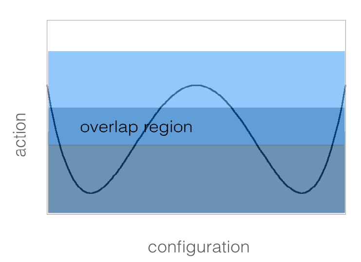
In order to solve this problem, one can use an adaptation of the replica exchange method Replica , as first proposed in Replicawl . The idea is that instead of dividing the whole energy interval in contiguous sub-intervals overlapping only in one point (in the following simply referred to as contiguous intervals), one can divide it in sub-intervals overlapping in a finite energy region (this case will be referred to as overlapping intervals). With the latter prescription, after a fixed number of iterations of the Robbins-Monro procedure, we can check whether in any pairs of overlapping intervals ) the energy of both the corresponding configurations is in the common region. For pairs fulfilling this condition, we can propose an exchange of the configurations with a Metropolis probability
| (49) |
where and are the values of the parameter at the current -th iterations of the Robbins-Monro procedure respectively in intervals and and () is the value of the energy of the current configuration () of the replica in the interval (). If the proposed exchange is accepted, and . With repeated exchanges of configurations from neighbour intervals, the system can now travel through all configuration space. A schematic illustration of how this mechanism works is provided in Fig. 1.
As already noticed in Replicawl , the replica exchange step is amenable to parallelisation and hence can be conveniently deployed in calculations on massively parallel computers. Note that the replica exchange step adds another tunable parameter to the algorithm, which is the number of configurations swaps during the Monte-Carlo simulation at a given Monte-Carlo step. A modification of the LLR algorithm that incorporates this step can be easily implemented.
2.6 Reweighting with the numerical density of states
In order to screen our approach outlined in subsections 2.2 and 2.3 for ergodicity violations and to propose an efficient procedure to calculate any observable once an estimate for the density of states has been obtained, as an alternative to the replica exchange method discussed in the previous section, we here introduce an importance sampling algorithm with reweighting with respect to the estimate . This algorithm features short correlation times even near critical points. Consider for instance a system described by the canonical ensemble. We define a modified Boltzmann weight as follows:
| (50) |
Here and are two values of the energy that are far from the typical energy of interest :
| (51) |
If conventional Monte-Carlo simulations can be used for numerical studies of the given system, we can chose and from the conditions
| (52) |
If importance sampling methods are inefficient or unreliable, and can be chosen to be the micro-canonical corresponding respectively to the density of states centred in and . These are outputs of our numerical determination . The two constants and are determined by requiring continuity of at and at :
| (53) |
Let be the correct density of state of the system. If , then for
| (54) |
and a Monte-Carlo update with weights drives the system in configuration space following a random walk in the energy. In practice, since is determined numerically, upon normalisation
| (55) |
and the random walk is only approximate. However, if is a good approximation of , possible free energy barriers and metastabilities of the canonical system can be successfully overcome with the weights (50). Values of observables for the canonical ensemble at temperature can be obtained using reweighting:
| (56) |
where denotes average over the canonical ensemble and average over the modified ensemble defined in (50). The weights guarantees ergodic sampling with small auto-correlation time for the configurations with energies such that , while suppressing to energy and . Hence, as long as for a given of the canonical system and the energy fluctuation are such that
| (57) |
the reweighting (56) does not present any overlap
problem. The role of and is to restrict the approximate
random walk only to energies that are physically interesting, in order
to save computer time. Hence, the choice of , and of the
corresponding , do not need to be fine-tuned, the
only requirement being that Eqs. (57) hold. These conditions
can be verified a posteriori. Obviously, choosing the smallest
interval where the conditions (57) hold
optimises the computational time required by the algorithm. The
weights (56) can be easily imposed using a metropolis or a
biased metropolis Bazavov:2005zy . Again, due to the absence of
free energy barriers, no ergodicity problems are expected to
arise. This can be checked by verifying that in the simulation there
are various tunnellings (i.e. round trips) between and
and that the frequency histogram of the energy is approximately
flat between and . Reasonable requirements are to have
tunnellings and an histogram that is flat within
15-20%. These criteria can be used to confirm that the numerically
determined is a good approximation of
. The flatness of the histogram is not influenced
by the of interest in the original multi-canonical
simulation. This is particularly important for first order phase
transitions, where traditional Monte-Carlo algorithms have a tunnelling
time that is exponentially suppressed with the volume of the
system. Since the modified ensemble relies on a random walk in energy,
the tunnelling time between two fixed energy densities is expected to
grow only as the square root of the volume.
This procedure of using a modified ensemble followed by
reweighting is inspired by the multi-canonical
method Berg:1992qua , the only substantial difference being the
recursion relation for determining the weights. Indeed for U(1)
lattice gauge theory a multi-canonical update for which the weights are
determined starting from a Wang-Landau recursion is discussed
in Berg:2006hh . We also note that the procedure used here
to restrict ergodically the energy interval between
and can be easily implemented also in the replica exchange
method analysed in the previous subsection.
3 Application to Compact U(1) Lattice Gauge Theory
3.1 The model
Compact U(1) Lattice Gauge Theory is the simplest gauge theory based on a Lie group. Its action is given by
| (58) |
where , with the gauge coupling, is a point of a d-dimensional lattice of size and and indicate two lattice directions, indicised from to (for simplicity, in this work we shall consider only the case ), plays the role of the electromagnetic field tensor: if we associate the compact angular variable with the link stemming from in direction ,
| (59) |
The path integral of the theory is given by
| (60) |
the latter identity defining the Haar measure of the U(1) group.
The connection with the framework of SU(N) lattice gauge theories is
better elucidated if we introduce the link variable
| (61) |
With this definition, can be rewritten as
| (62) |
with
the plaquette variable and is the complex conjugate of . Working with the variables allows us to show immediately that is invariant under U(1) gauge transformations, which act as
| (63) |
with a function defined on lattice points.
The connection with U(1) gauge theory in the continuum can be shown by introducing the lattice spacing and the non-compact gauge field , so that
| (64) |
Taking small and expanding the cosine leads us to
| (65) |
with the forward difference operator. In the limit , we finally find
| (66) |
with being the usual field strength tensor. This shows that in the classical limit becomes the Euclidean action of a free gas of photons, with interactions being related to the neglected lattice corrections. It is worth to remark that this classical continuum limit is not the continuum limit of the full theory. In fact, this classical continuum limit is spoiled by quantum fluctuations. These prevent the system from developing a second order transition point in the limit, which is a necessary condition to be able to remove the ultraviolet cutoff introduced with the lattice discretisation. The lack of a continuum limit is related to the fact that the theory is strongly coupled in the ultraviolet. Despite the non-existence of a continuum limit for Compact U(1) Lattice Gauge Theory, this lattice model is still interesting, since it provides a simple realisation of a weakly first order phase transition. This bulk phase transition separates a confining phase at low (whose existence was pointed out by Wilson Wilson:1974sk in his seminal work on Lattice Gauge Theory) from a deconfined phase at high , with the transition itself occurring at a critical value of the coupling . Rather unexpectedly at first side, importance-sampling Monte-Carlo studies of this phase transitions turned out to be demanding and not immediate to interpret, with the order of the transition having been debated for a long time (see e.g. Creutz:1979zg ; Lautrup:1980xr ; Bhanot:1981zg ; Jersak:1983yz ; Azcoiti:1991ng ; Bhanot:1992nf ; Lang:1994ri ; Kerler:1995va ; Jersak:1996mn ; Campos:1998jp ). The issue was cleared only relatively recently, with investigations that made a crucial use of supercomputers Arnold:2000hf ; Arnold:2002jk . What makes the transition difficult to observe numerically is the role played in the deconfinement phase transition by magnetic monopoles frolich:1987 , which condense in the confined phase frolich:1987 ; DiGiacomo:1997sm .
The existence of topological sectors and the presence of a transition with exponentially suppressed tunnelling times can provide robust tests for the efficiency and the ergodicity of our algorithm. This motivates our choice of Compact U(1) for the numerical investigation presented in this paper.
3.2 Simulation details
| (LLR) | (re-weighting) | |
|---|---|---|
| 1.006 | 0.60180(6) | 0.601714(8) |
| 1.008 | 0.60901(8) | 0.60906(1) |
| 1.010 | 0.6271(4) | 0.6274(1) |
| 1.01023 | 0.6349(5) | 0.6352(1) |
| 1.012 | 0.65685(5) | 0.65687(1) |
| 1.014 | 0.66018(4) | 0.660230(5) |
The study of the critical properties of U(1) lattice gauge theory is presented in this section. In order to test our algorithm, we investigated the behaviour of specific heath as function of the volume. This quantity has been carefully investigated in previous studies, and as such provides a stringent test of our procedure. In order to compare data across different sizes, our results will be often provided normalised to the number of plaquette .
We studied lattices sizes ranging from to and for each lattice size we computed the density of states in the entire interval (see Tab. 1). The rational behind the choice of the energy region is that it must be centred around the critical energy and it has to be large enough to study all the critical properties of the theory, i.e. every observable evaluated has to have support in this region and have virtually no correction coming from the choice of the energy boundaries.
| L | |||||
|---|---|---|---|---|---|
| 8 | 0.5722222 | 0.67 | 250 | 600 | 512 |
| 10,12,14,16,18,20 | 0.59 | 0.687777 | 200 | 400 | 512 |
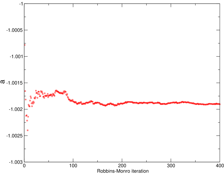
We divided the energy interval in steps of and for each of the sub-interval we have repeated the entire generation of the log-linear density of states function and evaluation of the observables times to create the bootstrap samples for the estimate of the errors. The values of the other tunable parameters of the algorithm used in our study are reported in Tab. 1. An example determination of one of the is reported in Fig. 3. The plot shows the rapid convergence to the asymptotic value and the negligible amplitude of residual fluctuations. Concerning the cost of the simulations, we found that accurate determinations of observables can be obtained with modest computational resources compared to those needed in investigations of the system with importance sampling methods. For instance, the most costly simulation presented here, the investigation of the lattice, was performed on 512 cores of Intel Westmere processors in about five days. This needs to be contrasted with the fact that in the early 2000’s only lattices up to could be reliably investigated with importance sampling methods, with the largest sizes requiring supercomputers Arnold:2000hf ; Arnold:2002jk .
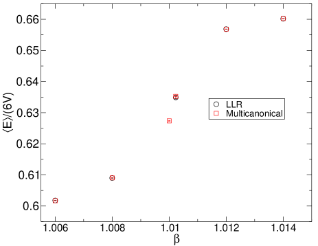
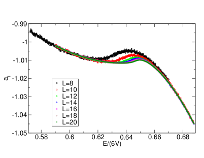
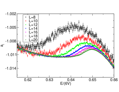
One of our first analyses was a screening for potential ergodicity violations with the LLR approach. As detailed in subsection 2.5, these can emerge for LLR simulations using contiguous intervals as it is the case for the U(1) study reported in this paper. To this aim, we calculated the action expectation value for a lattice for several values using the LLR method and using the re-weighting with respect to the estimate . Since the latter approach is conceptually free of ergodicity issues, any violations by the LLR method would be flagged by discrepancy. Our findings are summarised in Fig. 2 and the corresponding table. We find good agreement for the results from both methods. This suggests that topological objects do not generate energy barriers that trap our algorithm in a restricted section of configuration space. Said in other words, for this system the LLR method using contiguous interval seems to be ergodic.
3.3 Volume dependence of and computational cost of the algorithm
As first investigation we have performed a study of the scaling properties of the as function of the volume. In Fig. 4 we show the behaviour of the with the lattice volume. The estimates are done for a fixed , where the chosen value for the ratio fulfils the request that within the errors all our observables are not varying for (we report on the study of in section 3.5). As it is clearly visible from the plot the data are scaling toward a infinite volume estimate of the for fixed energy density.
As mentioned before, the issue facing importance sampling studies at first order phase transitions are connected with tunnelling times that grow exponentially with the volume. With the LLR method, the algorithmic cost is expected to grow with the size of the system as , where one factor of comes from the increase of the size and the other factor of comes from the fact that one needs to keep the energy interval per unit of volume fixed, as in the large-volume limit only intensive quantities are expected to determine the physics. One might wonder whether this apparently simplistic argument fails at the first order phase transition point. This might happen if the dynamics is such that a slowing down takes place at criticality. In the case of Compact U(1), for the range of lattice sizes studied here, we have found that the computational cost of the algorithm is compatible with a quadratic increase with the volume.
3.4 Numerical investigation of the phase transition
Using the density of states it is straightforward to evaluate, by direct integration (see subsection 2.3), the expectation values of any power of the energy and evaluate thermodynamical quantities like the specific heat
| (67) |
As usual we define the pseudo-critical coupling such as the coupling at which the peak of the specific heat occurs for a fixed volume. The peak of the specific heat has been located using our numerical procedure and the error bars are computed using the bootstrap method. Our results are summarised in Tab. 2 with a comparison with the values in Arnold:2000hf . Once again, the agreement testify the good ergodic properties of the algorithm.
| L | present method | reference values |
|---|---|---|
| 8 | 1.00744(2) | 1.00741(1) |
| 10 | 1.00939(2) | 1.00938(2) |
| 12 | 1.010245(1) | 1.01023(1) |
| 14 | 1.010635(5) | 1.01063(1) |
| 16 | 1.010833(4) | 1.01084(1) |
| 18 | 1.010948(2) | 1.010943(8) |
| 20 | 1.011006(2) |
Using our data it is possible to make a precise estimate of the infinite volume critical beta by means of a finite size scaling analysis. The finite size scaling of the pseudo-critical coupling is given by
| (68) |
where is the critical coupling. We fit our data with the function in Eq. (68), the results are reported in Tab. 3.
| 14 | 1 | 1.011125(3) | 0.91 |
|---|---|---|---|
| 12 | 1 | 1.011121(3) | 2.42 |
| 12 | 2 | 1.011129(4) | 0.67 |
| 10 | 1 | 1.011116(5) | 7.44 |
| 10 | 2 | 1.011127(3) | 0.60 |
| 8 | 1 | 1.011093(5) | 90.26 |
| 8 | 2 | 1.011126(2) | 0.62 |
Another quantity easily accessible is the latent heat, this quantity can be related to the height of the peak of the specific heat at the critical temperature through:
| (69) |
where is the latent heat. The results for this observable are reported in Tab. 4. We fit the result with Eq. (69), see Tab. 5.
| L | peak present work | peak from Arnold:2000hf |
|---|---|---|
| 8 | 0.000551(2) | 0.000554(1) |
| 10 | 0.000384(2) | 0.000385(1) |
| 12 | 0.0002971(11) | 0.000298(1) |
| 14 | 0.0002537(8) | 0.000254(1) |
| 16 | 0.0002272(7) | 0.000226(2) |
| 18 | 0.0002097(5) | 0.000211(2) |
| 20 | 0.0002007(4) |
| 14 | 1 | 0.02712(9) | 4.6 |
| 12 | 1 | 0.0273(2) | 31 |
| 12 | 2 | 0.02688(7) | 1.4 |
| 10 | 1 | 0.0276(2) | 74 |
| 10 | 2 | 0.02710(12) | 9.7 |
| 10 | 3 | 0.02681(9) | 1.4 |
| 8 | 1 | 0.0281(4) | 335 |
| 8 | 2 | 0.02731(15) | 26 |
| 8 | 3 | 0.02703(11) | 6.7 |
The latent heat can be obtained also from the knowledge of the location of the peaks of the probability density at (of infinite volume), indeed in this case the latent heat is equal to energy gap between the peaks. This direct measure can be used as crosscheck of the previous analysis. In the language of the density of states the probability density is simply given by
| (70) |
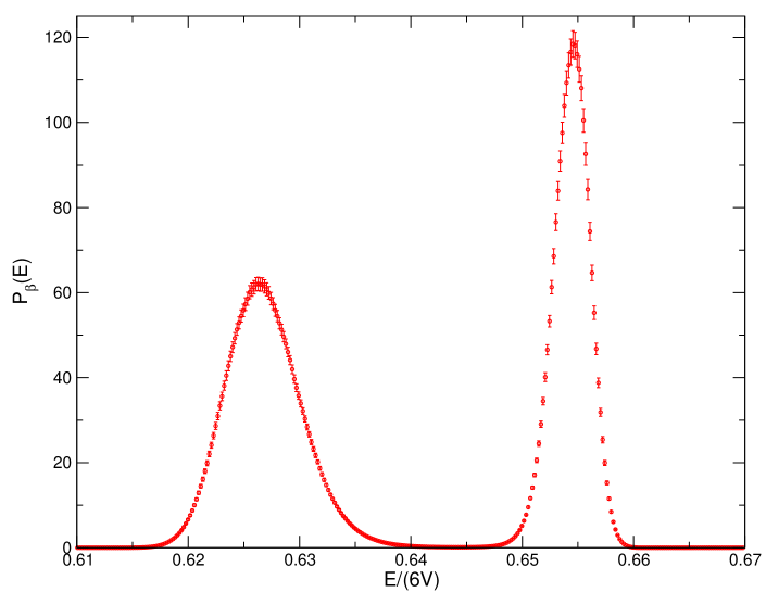
We have performed the study of the location in energy of the two peaks of and we have reported them in Tab. 6. Also in this case we have performed a finite size scaling analysis to extract the infinite volume behaviour:
| (71) |
A fit of the values in Tab. 6 yields and . The latent heat can be evaluated as which is in perfect agreement with the estimates obtained by studying the scaling of the specific heath.
| 12 | 0.6263(5) | 0.65580(14) |
|---|---|---|
| 14 | 0.6264(2) | 0.65532(5) |
| 16 | 0.6272(2) | 0.65512(4) |
| 18 | 0.6274(4) | 0.65495(6) |
| 20 | 0.6275(2) | 0.65491(7) |
3.5 Discretisation effects
In this section we want to address the dependence of our observables from the size of energy interval . In order to quantify this quantity we studies the dependence of the peak of the specific heat with for various lattice sizes, namely . In table 7 we report the lattice sizes and the corresponding used to perform such investigation. For each pair of and volume reported we have repeated all our simulations and analysis with the same simulation parameters reported in Tab. 1.
| L | |
|---|---|
| 10 | 8, 16, 32, 64, 128, 512 |
| 12 | 8, 16, 20, 32, 64, 128, 512 |
| 14 | 16, 32, 64, 512 |
| 16 | 16, 32, 64, 128, 512 |
The choice of the specific heat as an observable for such investigation can be easily justified: we found that specific heath is much more sensible to the discretisation effects with respect to other simpler observables such as the plaquette expectation value. In Fig. 6 we report an example of such study relative to .
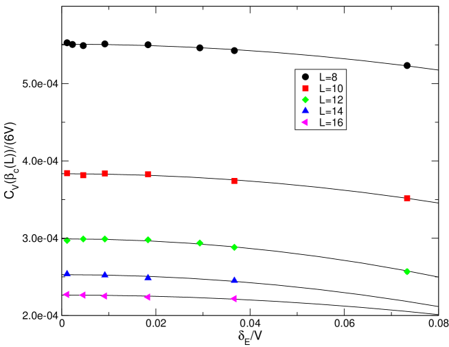
We can confirm that all our data are scaling with quadratic law in consistent with our findings in subsection 2.3. Indeed by fitting our data with a form
| (72) |
we found for all lattice sizes we investigated. We report in in Tab.(8) the values of . Note that the numerical values used in our finite size scaling analysis of the peak of presented in the previous section are compatible with the results extrapolated to obtained here.
| 8 | -3.1(2) |
|---|---|
| 10 | -5.9(4) |
| 12 | -1.8(1) |
| 14 | -4(1) |
| 16 | -9(3) |
4 Discussion, conclusions and future plans
The density of states is a measure of the number of configurations on the hyper-surface of a given action . Knowing the density of states relays the calculation of the partition function to performing an ordinary integral. Wang-Landau type algorithms perform Markov chain Monte-Carlo updates with respect to while improving the estimate for during simulations. The LLR approach, firstly introduced in Langfeld:2012ah , uses a non-linear stochastic equation (see (17)) for this task and is particularly suited for systems with continuous degrees of freedom. To date, the LLR method has been applied to gauge theories in several publications, e.g. Langfeld:2014nta ; Langfeld:2013xbf ; Pellegrini:2014gha ; Gattringer:2015lra , and has turned out in practice to be a reliable and robust method. In the present paper, we have thoroughly investigated the foundations of the method and have presented high-precision results for the U(1) gauge theory to illustrate the excellent performance of the approach.
Two key features of the LLR approach are:
-
(i)
It solves an overlap problem in the sense that the method can specifically target the action range that is of particular importance for an observable. This range might easily be outside the regime for which standard MC methods would not be able to produce statistics.
-
(ii)
It features exponential error suppression: although the density of states spans many orders of magnitude, its linear approximation has a nearly-constant relative error (see subsection 2.2) and the numerical determination of preserves this level of accuracy.
We point out that feature (i) is not exclusive of the LLR method, but is quite generic for multi-canonical techniques Berg:1992qua , Wang-Landau type updates Wang:2001ab or hybrids thereof Berg:2006hh .
Key ingredient for the LLR approach is the double-bracket expectation value Langfeld:2012ah (see (13)). It appears as a standard Monte-Carlo expectation value over a finite action interval of size and with the density of states as a re-weighting factor. The derivative of the density of states emerges from an iteration involving these Monte-Carlo expectation values. This implies that their statistical error interferes with the convergence of the iteration. This might introduce a bias preventing the iteration to converge to the true derivative . We resolved this issue by using the Robbins-Monro formalism robbins1951 : we showed that a particular type of under-relaxation produces a normal distribution of potential values with the mean of this distribution coinciding with the correct answer (see subsection 2.2).
In this paper, we also addressed two concerns, which were raised in the wake of the publication Langfeld:2012ah :
-
(1)
The LLR simulations restrict the Monte-Carlo updates to a finite action interval and might therefore be prone to ergodicity violations.
-
(2)
The LLR approach seems to be limited to the calculation of action dependent observables only.
To address the first issue, we have proposed in subsections 2.5 and 2.6 two procedures that are conceptually free of ergodicity violations. The first method is based upon the replica exchange method Replica ; Replicawl : using overlapping action ranges during the calculation of the double-bracket expectation values offers the possibility to exchange the configurations of neighbouring action intervals with appropriate probability (see subsection 2.5 for details). The second method is a standard Monte-Carlo simulation but with the inverse of the estimated density of states, i.e., , as re-weighting factor. The latter approach falls into the class of ergodic Monte-Carlo update techniques and is not limited by a potential overlap problem: if the estimate is close to the true density , the Monte-Carlo simulation is essentially a random walk in configuration space sweeping the action range of interest.
To address issue (2), we firstly point out that the latter re-weighting approach produces a sequence of gauge field configurations that can be used to calculate any observable by averaging with the correct weight. Secondly, we have developed in subsection 2.2 the formalism to calculate any observable by a suitable sum over a combination of the density of states and double-bracket expectation values involving the observable of interest. We were able to show that the order of convergence (with the size of the action interval) for these observables is the same as for itself (i.e., ).
In view of the features of the density of states approach, our future plans naturally involve investigations that either are enhanced by the direct access to the partition function (such as the calculation of thermodynamical quantities) or that are otherwise hampered by the overlap problem. These, most notably, include complex action systems such as cold and dense quantum matter. The LLR method is very well equipped for this task since it is based upon Monte-Carlo updates with respect to the positive (and real) estimate of the density of states and features exponential error suppression which might beat the resulting overlap problem. Indeed, a strong sign problem was solved by LLR techniques using the original degrees of freedom of the spin model Langfeld:2014nta ; Gattringer:2015lra . We are currently extending these investigations to other finite density gauge theories. QCD at finite densities for heavy quarks (HDQCD) is work in progress. We have plans to extend the studies to finite density QCD with moderate quark masses.
Acknowledgements.
We thank Ph. de Forcrand for discussions on the algorithm that lead to the material reported in Subsect. 2.6. The numerical computations have been carried out using resources from HPC Wales (supported by the ERDF through the WEFO, which is part of the Welsh Government) and resources from the HPCC Plymouth. KL and AR are supported by the Leverhulme Trust (grant RPG-2014-118) and STFC (grant ST/L000350/1). BL is supported by STFC (grant ST/L000369/1). RP is supported by STFC (grant ST/L000458/1).Appendix A Reference scale and volume scaling
Here, we will present further details on the scaling of the density of states with the volume of our system. To this aim, we will work in the regime of a finite correlation length such that the volume . In the case of particle physics, is a multiple of the inverse mass of the lightest excitation of the theory. In this subsection, we do not address the case of a correlation length comparable or larger than the size of the system, as it might occur near a second order phase transition.
Under these assumptions, the total action appears as a sum over uncorrelated contributions:
| (73) |
where the dimensionless variable is the volume in units of the (physical) correlation length. To ease the notation, we will assume that the densities and are normalised to one. Taking advantage of the above observation, we can introduce the probability distribution for the uncorrelated domains:
| (74) |
Representing the -function as Fourier integral, we find
| (75) | |||||
The latter equation is the starting point for a study of moments and cumulants of the action expectation values and their scaling with the volume.
Cumulants of the action are defined by:
| (76) |
Inserting (75) into (76), performing the and the integration leaves us with
| (77) |
where the volume independent cumulants are defined by
| (78) |
We here make the important observation that all cumulants are proportional to the “volume” rather than powers of it. Re-summing (78), i.e. using the identity
we find for in (75)
| (79) |
We perform the -integral by using the expansion
| (80) | |||||
| (81) | |||||
In next-to-leading order, we obtain (up to an additive constant):
| (82) |
Hence, we find for the inverse temperature
| (83) |
We therefore confirm that is an intrinsic quantity, i.e., volume independent. The curvature of at is given by
| (84) |
We therefore confirm the key thermodynamic assumptions in (5) by explicit calculation:
| (85) |
References
- (1) D. Landau and K. Binder, A Guide to Monte Carlo Simulations in Statistical Physics. Cambridge University Press, 2014.
- (2) N. Metropolis, A. W. Rosenbluth, M. N. Rosenbluth, A. H. Teller, and E. Teller, Equation of State Calculations by Fast Computing Machines, Journal of Chemical Physics 21 (1953) 1087–1092.
- (3) G. Aarts, Recent developments at finite density on the lattice, PoS CPOD2014 (2014) 012, [arXiv:1502.0185].
- (4) F. Wang and D. P. Landau, Efficient, multiple-range random walk algorithm to calculate the den sity of states, Phys. Rev. Lett. 86 (Mar, 2001) 2050–2053.
- (5) J. Xu and H.-R. Ma, Density of states of a two-dimensional model from the wang-landau algorithm, Phys. Rev. E 75 (Apr, 2007) 041115.
- (6) S. Sinha and S. Kumar Roy, Performance of Wang–Landau algorithm in continuous spi n models and a case study: Modified XY-model, Phys.Lett. A373 (2009) 308–314.
- (7) K. Langfeld, B. Lucini, and A. Rago, The density of states in gauge theories, Phys.Rev.Lett. 109 (2012) 111601, [arXiv:1204.3243].
- (8) K. Langfeld and B. Lucini, Density of states approach to dense quantum systems, Phys.Rev. D90 (2014), no. 9 094502, [arXiv:1404.7187].
- (9) C. Gattringer and P. Törek, Density of states method for the Z(3) spin model, arXiv:1503.0494.
- (10) K. Langfeld and J. M. Pawlowski, Two-color QCD with heavy quarks at finite densities, Phys.Rev. D88 (2013), no. 7 071502, [arXiv:1307.0455].
- (11) M. Guagnelli, Sampling the density of states, arXiv:1209.4443.
- (12) R. Pellegrini, K. Langfeld, B. Lucini, and A. Rago, The density of states from first principles, PoS LATTICE2014 (2015) 229, [arXiv:1411.0655].
- (13) H. Robbins and S. Monro, A stochastic approximation method, Ann. Math. Statist. 22 (09, 1951) 400–407.
- (14) M. Luscher and P. Weisz, Locality and exponential error reduction in numerical lattice gauge theory, JHEP 09 (2001) 010, [hep-lat/0108014].
- (15) R. H. Swendsen and J.-S. Wang, Replica monte carlo simulation of spin-glasses, Phys. Rev. Lett. 57 (Nov, 1986) 2607–2609.
- (16) T. Vogel, Y. W. Li, T. Wüst, and D. P. Landau, Scalable replica-exchange framework for wang-landau sampling, Phys. Rev. E 90 (Aug, 2014) 023302.
- (17) A. Bazavov and B. A. Berg, Heat bath efficiency with metropolis-type updating, Phys.Rev. D71 (2005) 114506, [hep-lat/0503006].
- (18) B. Berg and T. Neuhaus, Multicanonical ensemble: A New approach to simulate first order phase transitions, Phys.Rev.Lett. 68 (1992) 9–12, [hep-lat/9202004].
- (19) B. A. Berg and A. Bazavov, Non-Perturbative U(1) Gauge Theory at Finite Temperature, Phys.Rev. D74 (2006) 094502, [hep-lat/0605019].
- (20) K. G. Wilson, Confinement of Quarks, Phys.Rev. D10 (1974) 2445–2459.
- (21) M. Creutz, L. Jacobs, and C. Rebbi, Monte Carlo Study of Abelian Lattice Gauge Theories, Phys.Rev. D20 (1979) 1915.
- (22) B. Lautrup and M. Nauenberg, Phase Transition in Four-Dimensional Compact QED, Phys.Lett. B95 (1980) 63–66.
- (23) G. Bhanot, The Nature of the Phase Transition in Compact QED, Phys.Rev. D24 (1981) 461.
- (24) J. Jersak, T. Neuhaus, and P. Zerwas, U(1) Lattice Gauge Theory Near the Phase Transition, Phys.Lett. B133 (1983) 103.
- (25) V. Azcoiti, G. Di Carlo, and A. Grillo, Approaching a first order phase transition in compact pure gauge QED, Phys.Lett. B268 (1991) 101–105.
- (26) G. Bhanot, T. Lippert, K. Schilling, and P. Uberholz, First order transitions and the multihistogram method, Nucl.Phys. B378 (1992) 633–651.
- (27) C. Lang and T. Neuhaus, Compact U(1) gauge theory on lattices with trivial homotopy group, Nucl.Phys. B431 (1994) 119–130, [hep-lat/9407005].
- (28) W. Kerler, C. Rebbi, and A. Weber, Monopole currents and Dirac sheets in U(1) lattice gauge theory, Phys.Lett. B348 (1995) 565–570, [hep-lat/9501023].
- (29) J. Jersak, C. Lang, and T. Neuhaus, NonGaussian fixed point in four-dimensional pure compact U(1) gauge theory on the lattice, Phys.Rev.Lett. 77 (1996) 1933–1936, [hep-lat/9606010].
- (30) I. Campos, A. Cruz, and A. Tarancon, A Study of the phase transition in 4-D pure compact U(1) LGT on toroidal and spherical lattices, Nucl.Phys. B528 (1998) 325–354, [hep-lat/9803007].
- (31) G. Arnold, T. Lippert, K. Schilling, and T. Neuhaus, Finite size scaling analysis of compact QED, Nucl.Phys.Proc.Suppl. 94 (2001) 651–656, [hep-lat/0011058].
- (32) G. Arnold, B. Bunk, T. Lippert, and K. Schilling, Compact QED under scrutiny: It’s first order, Nucl.Phys.Proc.Suppl. 119 (2003) 864–866, [hep-lat/0210010].
- (33) Fröhlich, J. and Marchetti, P.A., Soliton quantization in lattice field theories, Communications in Mathematical Physics 112 (1987), no. 2 343–383.
- (34) A. Di Giacomo and G. Paffuti, A Disorder parameter for dual superconductivity in gauge theories, Phys.Rev. D56 (1997) 6816–6823, [hep-lat/9707003].