Combining allele frequency uncertainty and population substructure corrections in forensic DNA calculations

Abstract

In forensic DNA calculations of relatedness of individuals and in DNA mixture analyses, two sources of uncertainty are present concerning the allele frequencies used for evaluating genotype probabilities when evaluating likelihoods. They are: (i) imprecision in the estimates of the allele frequencies in the population by using an inevitably finite database of DNA profiles to estimate them; and (ii) the existence of population substructure. Green and Mortera (2009) showed that these effects may be taken into account individually using a common Dirichlet model within a Bayesian network formulation, but that when taken in combination this is not the case; however they suggested an approximation that could be used. Here we develop a slightly different approximation that is shown to be exact in the case of a single individual. We demonstrate the closeness of the approximation numerically using a published database of allele counts, and illustrate the effect of incorporating the approximation into calculations of a recently published statistical model of DNA mixtures.

Keywords

Genotype probabilities; uncertain allele frequency; population substructure; DNA mixtures.

1 Introduction

In a recent publication, Cowell et al. (2015) presented a statistical model for the quantitative peak information obtained from an electropherogram of one or more forensic DNA samples. The model incorporates stutter and dropout artefacts, and allows for the presence of multiple unknown individuals contributing to the samples. Using likelihood maximization, the model can be used to compare hypothetical assumptions about the contributors to the DNA samples, and for deconvolution of the mixture samples to generate a set of joint genotypes of hypothesized untyped contributors that is ranked by likelihood.

The model of Cowell et al. (2015) assumes that the set of alleles in the population entering the likelihood calculations are in Hardy-Weinberg equilibrium, that is, there is no population substructure. It also assumes that the population allele frequencies are precisely known. Neither assumption is valid for real casework. In the discussion section to Cowell et al. (2015), several contributors pointed to the need to accommodate these issues. Of particular interest for this paper is the contribution from Green and Mortera, and the contribution from Tvedebrink, Eriksen and Morling.

The comments from the latter contributors are presented in more detail in (Tvedebrink et al., 2015), and deal with incorporating population substructure into the mixture calculations using the Balding-Nichols correction (Balding and Nichols, 1994). They show that a Dirichlet-multinomial distribution may be incorporated into an extension of the Markov model of allele probabilities of (Cowell et al., 2015) in order to take account of the Balding-Nichols $\theta$ correction. Green discussed ongoing work with Mortera, extending earlier work in (Green and Mortera, 2009), for modelling the uncertainty in allele frequencies arising from using observed frequency counts for alleles in a (finite) database. Curiously, this also leads to a Dirichlet-multinomial distribution with parameters depending on the total database size and a Dirichlet prior parameter for allele frequencies. In particular, the same extension of the Markov model presented by Tvedebrink et al. (2015) for population substructure may be used instead to model the uncertain allele frequency (UAF) by reinterpreting the Balding-Nichols $\theta$ parameter as a function of the database size. The common occurrence of the Dirichlet-multinomial distribution for separately modelling either population substructure or uncertainty in allele frequency was shown by Green and Mortera (2009) in terms of their Bayesian network model. They show that in combination they do not follow a Dirichlet-multinomial distribution when there are three or more founding alleles for a locus, but suggest a first order additive approximation that could be used for combining the two sources of uncertainty with the Dirichlet-multinomial framework.

This paper revisits the approximation suggested by Green and Mortera (2009) for combining corrections for population substructure and uncertain allele frequency. We develop a closed form formula slightly different to their additive approximation that is exact for a single person and which we propose may be used as an approximation for problems involving more than one person. We examine the numerical accuracy of the approximation using a published population database, and how it affects likelihoods in the mixture example examined in (Cowell et al., 2015). We begin by summarizing the Dirichlet models for each source of uncertainty taken separately, and then consider them in combination.

2 Dirichlet modelling of population substructure correction

A commonly applied probability model to take account of shared ancestry in a population is the $\theta$ correction of Balding and Nichols (1994). In this model, the distribution of alleles in the population is assumed to be known. To account for the co-ancestry of individuals, a small parameter $\theta$ is introduced which perturbs the genotype probabilities away from those obtained under Hardy-Weinberg equilibrium. For example, if an allele of type $a$ occurs in the population with probability $p_{a}$, then under Hardy-Weinberg equilibrium the probability for a randomly selected individual having the homozygotic genotype $(a,a)$ would be $p_{a}^{2}$, but with the $\theta$ adjustment it is instead $p_{a}(\theta+(1-\theta)p_{a}$. If $\theta=0$ we recover the Hardy-Weinberg values $p_{a}^{2}$. Values of $\theta$ used in forensic calculations are typically in the range 0.01-0.03.

More generally, for a given locus denote the allele frequencies in the population by the vector $\mathbf{p}=(p_{1},p_{2},\ldots,p_{K})$ for the $K$ alleles $(A_{1},A_{2},\ldots,A_{K})$. The probability of randomly selecting one allele of type $A_{k}$ is $p_{k}$. The probability of randomly selecting a second allele of the same type, given we have seen already selected it once, is

$$\frac{\theta+(1-\theta)p_{k}}{1}$$

The probability of randomly selecting a third allele of the same type, given we have selected two copies, is

$$\frac{2\theta+(1-\theta)p_{k}}{1+\theta}$$

In general the probability of seeing an $a_{k}$-th allele of this type given we have seen $a_{k}-1$ of that type previously, is

$$\frac{(a_{k}-1)\theta+(1-\theta)p_{k}}{(a_{k}-1)\theta+1-\theta}.$$

Hence the probability of seeing $a_{k}$ alleles of type $A_{k}$ will be

$$\prod_{j_{k}=1}^{a_{k}}\frac{(j_{k}-1)\theta+(1-\theta)p_{k}}{(j_{k}-1)\theta+1-\theta}$$

Taking through the factor of $\theta$ top and bottom (assuming that $\theta>0$), and writing $\phi=(1-\theta)/\theta$, this may be rewritten as

$$\prod_{j_{k}=1}^{a_{k}}\frac{j_{k}-1+\phi p_{k}}{j_{k}-1+\phi}$$

Finally, taken over the set of alleles in a set of $I$ genotypes denoted by $g$ which have a total of $a_{k}$ alleles of type $A_{k}$ on the locus, this result extends to

$$P(g|\mathbf{p})=2^{h}\frac{\prod_{k}\prod_{j_{k}=1}^{a_{k}}(j_{k}-1+\phi p_{k})}{\prod_{j=1}^{2I}(j-1+\phi)},$$ (1)

where $h$ the number of heterozygous genotypes amongst the $I$ genotypes $g$.

3 Dirichlet modelling of uncertain allele frequency

A Bayesian approach to dealing with uncertainty in the population allele frequencies $\pi(\textbf{p})$ is to treat them as random variables with a Dirichlet prior distribution:

p $$=(p_{1},p_{2},\ldots,p_{k})\sim\mbox{Dir}(\alpha_{1},\alpha_{2},\ldots,\alpha_{K}),$$

$$\pi(\textbf{p}) =\Gamma(\alpha)\prod_{i=1}^{K}\frac{p_{i}^{\alpha_{i}-1}}{\Gamma(\alpha_{i})},$$

where each $p_{i}\geq 0$, $\sum p_{i}=1$ and $\alpha=\sum\alpha_{i}$.

The $\alpha_{i}$ are commonly taken to be the observed allele counts in a database (so for a database of $M$ alleles this would give $\sum\alpha_{i}=M$). In this case $\widehat{p_{i}}=\alpha_{i}/M$ would be the proportion of alleles of types $A_{i}$ of the locus in the database, and

$$\mbox{Dir}(\alpha_{1},\alpha_{2},\ldots,\alpha_{K})\equiv\mbox{Dir}(M\widehat{p_{1}},M\widehat{p_{2}},\ldots,M\widehat{p_{K}}).$$

An alternative is to give the $\alpha_{i}$ values representing a prior belief about the occurrence of alleles in the population before the database is observed. Two common suggestions for the values of the prior parameters $\alpha_{i}$ are to set $\alpha_{i}=1/K$, or to set $\alpha_{i}=1$. Curran and Buckleton (2011) argue in favour of setting each $\alpha_{i}=1/K$. The observed allele counts $\textbf{m}=(m_{1},m_{2},\ldots,m_{K})$ of alleles in the database for the locus are used to update this prior, on the assumption that the alleles in the database are independent and multinomially distributed given p. This leads to a posterior density also of Dirichlet type:

$$\pi(\textbf{p} |\textbf{m})=\mbox{Dir}(\alpha_{1}+m_{1},\alpha_{2}+m_{2},\ldots,\alpha_{K}+m_{K})$$

$$\equiv\mbox{Dir}(M\widehat{p_{1}},M\widehat{p_{2}},\ldots,M\widehat{p_{K}})$$

where now $M=\sum_{i}{\alpha_{i}+m_{i}}$ and $\widehat{p_{i}}=E(p_{i}|\textbf{m})$.

Whichever approach is used, we have a distribution of alleles that takes into account the observed alleles in the database of the form:

$$\pi(\textbf{p}|\textbf{m})=\mbox{Dir}(M\widehat{p_{1}},M\widehat{p_{2}},\ldots,M\widehat{p_{K}}).$$

Genotype probabilities are then obtained by averaging over this distribution:

$$P(g) =\int P(g|\mathbf{p})d\pi(\mathbf{p}|m)$$

$$=2^{h}\int\prod_{k}p_{k}^{a_{k}}d\pi(\mathbf{p}|m)$$

$$=2^{h}\frac{\Gamma(M)}{\Gamma(M+2I)}\prod_{k}\frac{\Gamma(M\widehat{p_{k}}+a_{k})}{\Gamma(M\widehat{p_{k}})}$$

$$=2^{h}\frac{\prod_{k}\prod_{j_{k}=1}^{a_{k}}(M\widehat{p_{k}}+j_{k}-1)}{\prod_{j=1}^{2I}(M+j-1)}$$ (2)

Note that the right-hand-side of (2) is the same as on the right-hand-side of (1) if we identify $M\equiv\phi=(1-\theta)/\theta$, (so that $\theta\equiv 1/(M+1)$), as was pointed out by Green and Mortera (2009).

In other words, the use of Bayesian averaging with a Dirichlet prior to take account of uncertainty in allele frequencies in the population arising from using estimates from a finite database, is numerically equivalent to a Balding-Nichols $\theta$ correction for co-ancestry on setting $\theta=1/(M+1)$ and using the $\widehat{p_{i}}$ as if they are the true population allele frequencies. If in addition we take each of the $\alpha_{i}=0$ (for the Dirichlet prior before the database allele counts are incorporated), then $M$ is the size of the database and the $\widehat{p_{i}}$ are the observed proportions of the alleles in the database.

4 A notational aside

Before proceeding to the consideration of allele frequency uncertainty combined with substructure correction, we define the following function:

$$f(x;n)=\prod_{j=1}^{n}(j-1+x)$$ (3)

Expanding $f(x;n)$ as a power series in $x$, we denote the coefficients of the power of $x^{j}$ by $c(j,n)$ so that $f(x;n)=\sum_{j=0}^{n}c(j,n)x^{j}$. We define $c(0,0)=1$, and for every integer $j>0$ we have that $c(0,j)=0$. It is not hard to show the following low-order expansions of $f(x;n)$ for $n$ values up to $n=6$:

$$f(x;0) =1$$

$$f(x,1) =x$$

$$f(x;2) =x+x^{2}$$

$$f(x;3) =2x+3x^{2}+x^{3}$$

$$f(x;4) =6x+11x^{2}+6x^{3}+x^{4}$$

$$f(x;5) =24x+50x^{2}+35x^{3}+10x^{4}+x^{5}$$

$$f(x;6) =120x+274x^{2}+225x^{3}+85x^{4}+15x^{5}+x^{6}$$

5 Combining UAF and $\theta$ corrections

Our proposed method for combining UAF with $\theta$ correction for evaluating a joint genotypes probability is to calculate the joint genotype probability using the $\theta$ correction given allele frequencies $\mathbf{p}$, and then to integrate the result with respect to a Dirichlet for the population allele frequencies $\mathbf{p}$ in order to take account of uncertainty in their population values.

Now given the allele frequencies, the genotype probability for the (joint) genotype $g$ (of one or more individuals) taking into account co-ancestry is given by (1):

$$P(g|\mathbf{p})=2^{h}\frac{\prod_{k}\prod_{j_{k}=1}^{a_{k}}(j_{k}-1+\phi p_{k})}{\prod_{j=1}^{2I}(j-1+\phi)}.$$

$$P(g)=E[P(g|\mathbf{p})] =2^{h}\int\frac{\prod_{k}\prod_{j_{k}=1}^{a_{k}}(j_{k}-1+\phi p_{k})}{\prod_{j=1}^{2I}(j-1+\phi)}d\pi(\mathbf{p})$$ (4)

Thus we need to evaluate the multiple integral

$$E\left[\frac{\prod_{k}\prod_{j_{k}=1}^{a_{k}}(j_{k}-1+\phi p_{k})}{\prod_{j=1}^{2I}(j-1+\phi)}\right]=\frac{\Gamma(\phi)}{\Gamma(\phi+2I)}\int\prod_{k}\prod_{j_{k}=1}^{a_{k}}(j_{k}-1+\phi p_{k})d\pi(\mathbf{p}).$$

We may rewrite the above expectation in terms of the $f$ function introduced earlier:

$$E\left[\frac{\prod_{k}\prod_{j_{k}=1}^{a_{k}}(j_{k}-1+\phi p_{k})}{\prod_{j=1}^{2I}(j-1+\phi)}\right] =\frac{\Gamma(\phi)}{\Gamma(\phi+2I)}\int\prod_{k}f(\phi p_{k},a_{k})d\pi(\mathbf{p})$$

$$=\frac{\Gamma(\phi)}{\Gamma(\phi+2I)}\int\prod_{k}\left(\sum_{j_{k}=0}^{a_{k}}c(j_{k},a_{k})(\phi p_{k})^{j_{k}}\right)d\pi(\mathbf{p})$$

In the case where the set of genotypes $g$ is that of a single person, the product in the integral has just one term and is readily evaluated. We consider separately the two cases of a homozygous individual and a heterozygous individual.

Homozygous individual

If the individual is homozygous $(A_{k},A_{k})$, then the expectation involves the integral of $f(\phi p_{k},2)=\phi p_{k}+(\phi p_{k})^{2}$. If we denote the Dirichlet prior by $\mathbf{p}\sim\mbox{Dir}(s_{1},s_{2},\ldots,s_{K})$ where $s_{j}=M\widehat{p_{j}}$ and $s=\sum s_{j}=M$, then the expectation is given by:

$$\frac{\Gamma(\phi)}{\Gamma(\phi+2I)}\int\left(\phi p_{k}+(\phi p_{k})^{2}\right)d\pi(\mathbf{p}) =\frac{\Gamma(\phi)}{\Gamma(\phi+2I)}\left(\phi\frac{s_{k}}{s}+\phi^{2}\frac{s_{k}(s_{k}+1)}{s(s+1)}\right)$$

$$=\frac{1}{\phi(\phi+1)}\phi\frac{s_{k}}{s}\left(1+\phi\frac{s_{k}+1}{s+1}\right)$$

$$=\frac{s_{k}}{s(\phi+1)}\left(1+\phi\frac{s_{k}+1}{s+1}\right)$$

We now using $\phi=(1-\theta)/\theta$, so that $1+\phi=1/\theta$, we rewrite the last line as

$$\frac{s_{k}}{s(\phi+1)}\left(1+\phi\frac{s_{k}+1}{s+1}\right) =\frac{s_{k}}{s}\left(\theta+(1-\theta)\frac{s_{k}+1}{s+1}\right)$$

$$=\frac{s_{k}}{s}\left(\theta+(1-\theta)\frac{s_{k}}{s}\frac{s}{s+1}+(1-\theta)\frac{1}{s+1}\right)$$

Now define

$$\tilde{\theta}=\theta+\frac{1-\theta}{s+1}.$$

Then we have that

$$1-\tilde{\theta}=(1-\theta)\frac{s}{s+1}$$

from which we obtain

$$\frac{s_{k}}{s}\left(\theta+(1-\theta)\frac{s_{k}}{s}\frac{s}{s+1}+(1-\theta)\frac{1}{s+1}\right)=\frac{s_{k}}{s}\left(\tilde{\theta}+(1-\tilde{\theta})\frac{s_{k}}{s}\right)$$

That is, given a Dirichlet distribution for allele frequencies $\mathbf{p}\sim\mbox{Dir}(s_{1},s_{2},\ldots,s_{K})$ to represent UAF, and the Balding-Nichols correction parameter $\theta$ to represent population substructure, then for a homozygous individual the probability associated with the genotype is the same as if using point estimates $\widehat{p_{k}}=s_{k}/s$ for the probabilities and using a substructure correction with a modified correction parameter $\tilde{\theta}=\theta+(1-\theta)/(s+1)$.

We shall now show the same is true if the individual is heterozygous.

Heterozygous individual

In the case of a heterozygous individual, with genotype $(A_{j},A_{k})$ and $j\neq k$, the integral will involve the product $2f(\phi p_{j},1)f(\phi p_{k},1)=2\phi^{2}p_{j}p_{k}$, thus:

$$2\frac{\Gamma(\phi)}{\Gamma(\phi+2I)}\int\phi^{2}p_{j}p_{k}d\pi(\mathbf{p}) =\frac{2}{\phi(\phi+1)}\phi^{2}\frac{s_{j}}{s}\frac{s_{k}}{s}$$

$$=\frac{2}{\phi+1}\phi\frac{s_{j}}{s}\frac{s_{k}}{s+1}$$

$$=\frac{2}{\phi+1}\phi\frac{s_{j}}{s}\frac{s_{k}}{s}\frac{s}{s+1}$$

$$=2\frac{s_{j}}{s}\frac{s_{k}}{s}\frac{\phi}{\phi+1}\frac{s}{s+1}$$

Now again using $\phi/(1+\phi)=1-\theta$, the last line may be rewritten:

$$2\frac{s_{j}}{s}\frac{s_{k}}{s}\frac{\phi}{\phi+1}\frac{s}{s+1}=2\frac{s_{j}}{s}\frac{s_{k}}{s}(1-\theta)\frac{s}{s+1}$$

If we again define $\tilde{\theta}=\theta+(1-\theta)/(s+1)$, then $1-\tilde{\theta}=(1-\theta)s/(s+1)$, hence the genotype probability can be written as

$$2\frac{s_{j}}{s}\frac{s_{k}}{s}(1-\tilde{\theta})$$

This is the what we would obtain by taking the $\widehat{p_{j}}={s_{j}}/{s}$ as the population allele frequencies and applied a population substructure correction using the transformed parameter $\tilde{\theta}=\theta+(1-\theta)/(s+1)$:

$$\frac{s_{j}}{s}\frac{s_{k}}{s}(1-\tilde{\theta})=2\widehat{p_{j}}\widehat{p_{k}}(1-\tilde{\theta}).$$

Thus we have shown that for the case of a single person, the genotype probability may be found when combining both UAF and population substructure corrections, by modifying the $\theta$ parameter value to take account of the size of the database by the transformation

$$\tilde{\theta}=\theta+\frac{1-\theta}{s+1}$$ (5)

and using $\tilde{\theta}$ from (5) in the Balding-Nichols correction in which the mean of the population allele frequency Dirichlet posterior is treated as being the population allele frequencies.

If we set $\theta=0$ in (5), then we obtain $\tilde{\theta}=1/(s+1)$, thus recovering the equivalence in Section 3 found by Green and Mortera (2009).

The above result does not extend to the case for two or more persons, although (5) may be used as an approximation. Green and Mortera (2009) suggested an alternative approximation for large $s$ ($M$ in their notation) and small $\theta$ which is “additive on the scale $M^{-1}=\theta/(1-\theta)$”, that is,

$$1/\phi_{GM}=1/\phi+1/s.$$

This is equivalent to the transformation of $\theta$ given by

$$\theta_{GM}=\frac{1+\theta(s-1)}{s+1-\theta}=\theta+\frac{(1-\theta)^{2}}{s+1-\theta}$$ (6)

6 Numerical investigation of approximation

6.1 Single person

We now illustrate the accuracy of the transformation (5), using population data for Caucasians on the marker vWA taken from Butler et al. (2003) shown in Table 1. (Similar results to those obtained below may be obtained for other markers.)

Table 1: Allele counts for a sample of US Caucasians for the marker vWA. These counts have been obtained by rescaling the normalized frequencies given in Butler et al. (2003) by the database size of $s=604$, and rounding the results to the nearest integer.

Allele	13	14	15	16	17	18	19	20	21
Count	1	57	67	121	170	121	63	3	1

We begin by looking at the distribution of the genotypes for a single individual. We do this by comparing the distribution of genotype probabilities for a single person calculated under (a) Hardy-Weinberg equilibrium, (b) the correction for UAF only, (c) the $\theta$ substructure correction only, and (d) the Green-Mortera approximation (6). Each is compared against the exact correction for both UAF and substructure in (5) by calculating for each possible genotype the ratio of the probabilities under each of the approximations to the exact value. Ideally the ratio should be 1. With the nine alleles of the vWA marker data in Table 1 there are 45 possible genotypes. For the comparisons we take $\theta=0.02$ and $s=604$, the database size. In Figure 1 are shown the empirical cumulative distributions of the ratio of the approximate to exact probabilities; the more the ratios are clustered around 1 the better the fit, as indicated by the vertical red lines. Note the smaller ranges for the subplots (c) and (especially) (d) compared to the subplots (a) and (b). In more detail, the following ranges of ratios were found for the data of each plot: (a) $(0.0712,1.0221)$; (b) $(0.1422,1.0204)$; (c) $(0.9304,1.0017)$; (d) $(0.998611,1.000033)$.

The plots indicate that the Green-Mortera approximation is excellent. This is confirmed by looking at the KL divergence between the approximate and exact genotype distributions; the values for the four approximations are respectively (a) 0.001376; (b) 0.001127; (c) 6.411e-06; and (d) 2.537e-09.

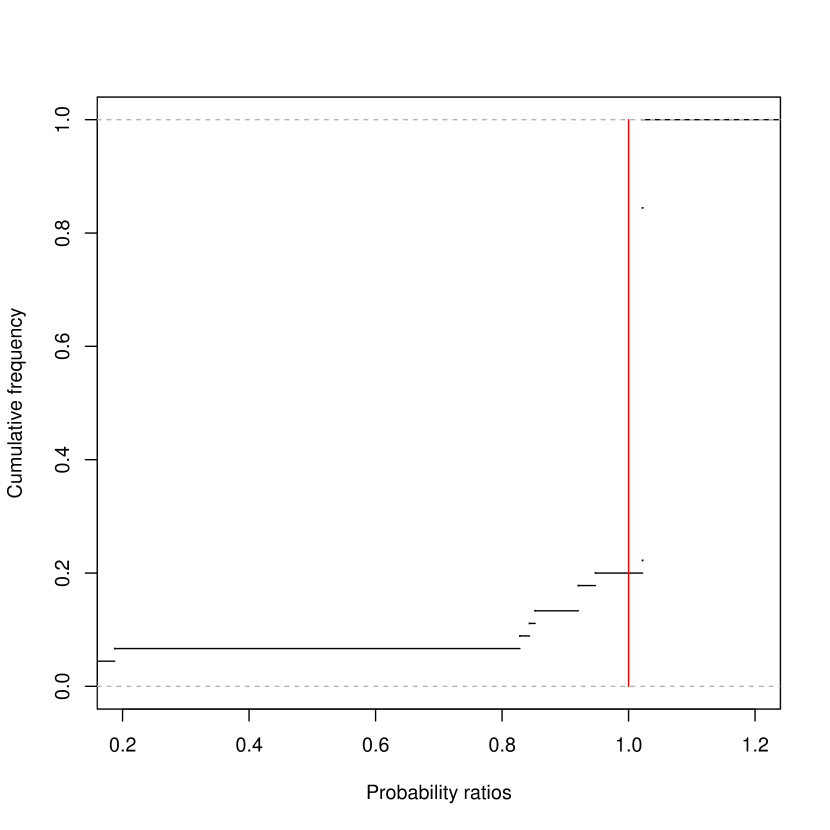
(a) Hardy-Weinberg

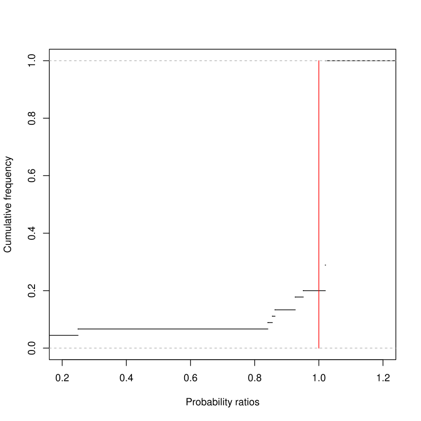
(b) UAF correction

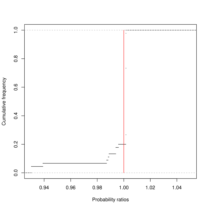
(c) Fst correction

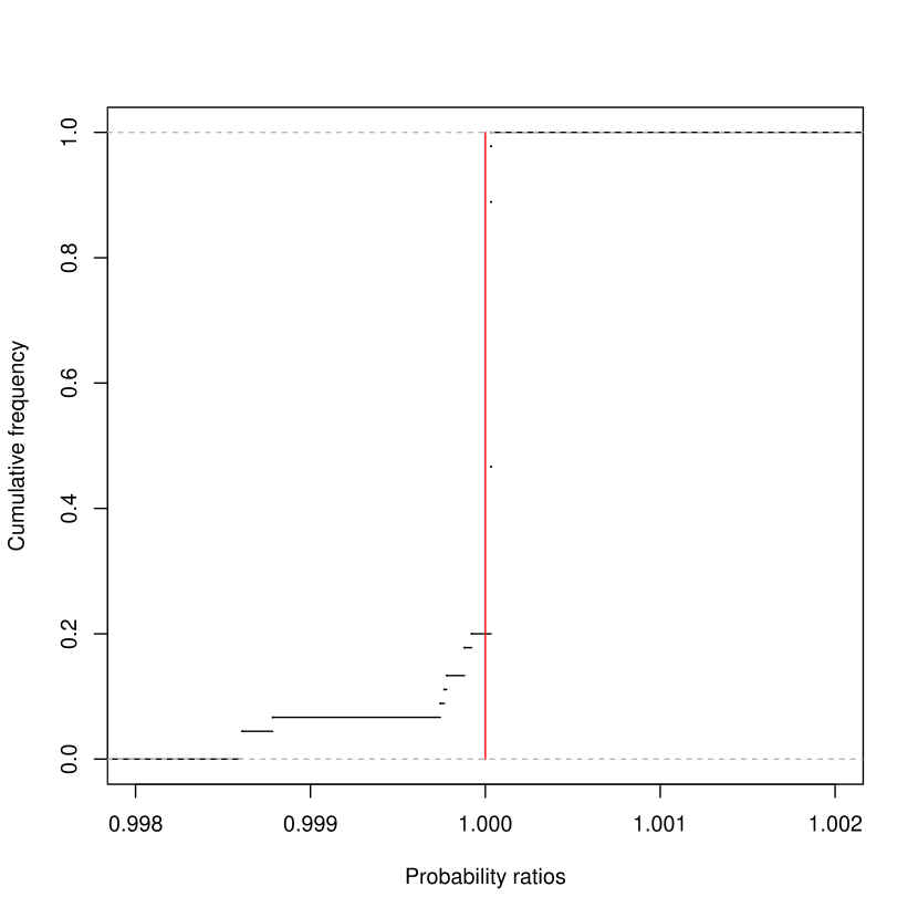
(d) Green-Mortera approximation

Figure 1: Empirical cumulative distribution functions of the ratios to exact single person genotype probabilities of corresponding genotype probabilities calculated under (a) Hardy-Weinberg equilibrium; (b) an uncertain allele frequency (finite database) correction without Fst correction; (c) Fst correction without finite database correction; (d) Green-Mortera approximation using finite database and Fst corrections. Note the much smaller range of ratios for plots (c) and (d). All plots are for the locus vWA. The database size is 604, and Fst correction where applied has $\theta=0.02$.

6.2 Two unrelated persons

In Figure 2 we compare the exact probabilities of the joint genotypes of two unrelated individuals (calculated with the aid of the $f(x;n)$ function in (3)) to various alternatives. Specifically, the exact genotype distribution is compared to genotype frequencies assuming (a) Hardy-Weinberg equilibrium, (b) a correction for uncertain allele frequency alone, (c) a correction for population substructure alone, and (d) the approximation using the exact single-person $\theta$ rescaling (5). (A plot using the correction (6) is very similar to (d) and is omitted.) As in Figure 1, the plots in Figure 2 show the empirical cumulative distributions of the ratio of the approximate to exact probabilities; the more the ratios are clustered around 1 the better the fit, as indicated by the vertical red lines. Again please note the smaller horizontal ranges for subplots (c) and (especially) (d) compared to plots (a) and (b). The following ranges of ratios of genotypes probabilities were found for the data of each plot: (a) $(0.0001,1.1383)$; (b) $(0.0018,1.1271)$; (c) $(0.8633,1.01)$; (d) $(0.995804,1.07377)$.

The plots indicate that the rescaled $\theta$ approximation (5) is excellent. This can be confirmed numerically by looking at the KL divergence between the approximate and exact solutions; the values for the four approximations are: (a) 0.008036; (b) 0.006552; (c) 3.6e-05; and (d) 4.9488e-08. (The KL divergence for the Green-Mortera approximation is 6.7575e-08, indicating the fit is not quite as good overall as that obtained using (5).) Similar results may be found for the joint genotypes of three unrelated individuals, details are omitted here.

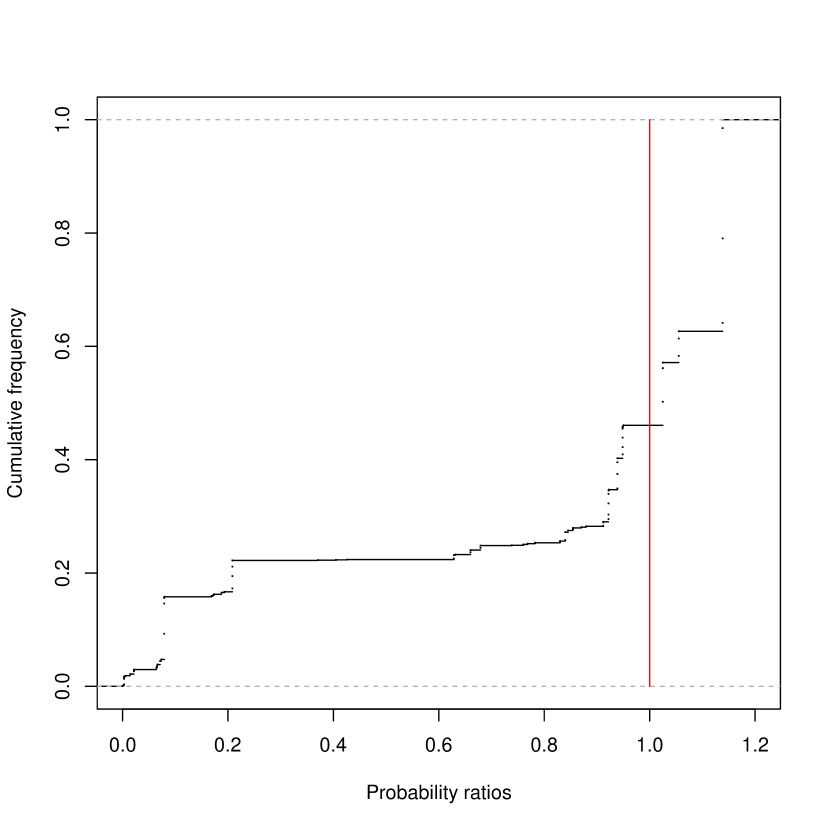
(a) Hardy-Weinberg

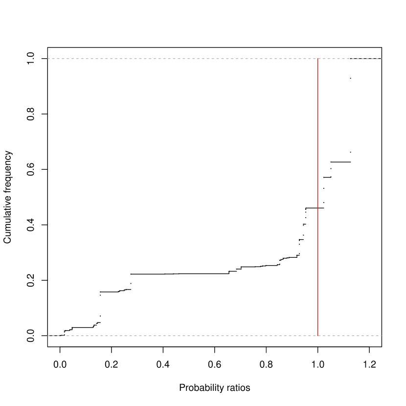
(b) UAF correction

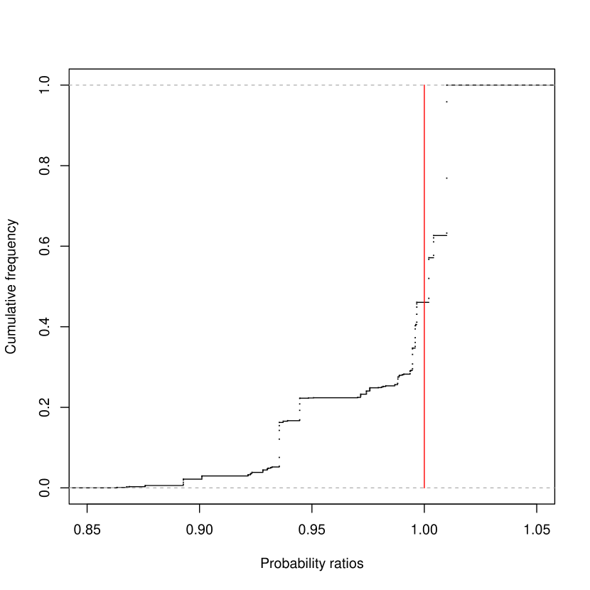
(c) Fst correction

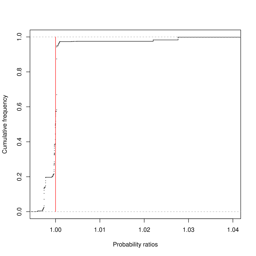
(d) Exact single-person approximation

Figure 2: Empirical cumulative distribution functions of the ratios to the exact joint genotype probabilities of two unrelated individuals of corresponding joint genotype probabilities calculated under (a) Hardy-Weinberg equilibrium; (b) an uncertain allele frequency (finite database) correction without Fst correction; (c) Fst correction without finite database correction; (d) approximation using exact adjusted theta value of single person. All plots are for the locus vWA. The database size is 604, and Fst correction where applied has $\theta=0.02$.

Figure 3 shows scatterplots of the genotypes ratio probabilities against the exact probabilities for the Hardy-Weinberg and adjusted $\theta$ approximations for the case of two unrelated individuals - (note the very different vertical scales). From this we see that the genotype probability ratios that are furthest away from unity tend to be associated with those genotype combinations having lower probabilities.

Figure 3: Probability ratios of each genotype possibility for two unrelated individuals calculated under HW equilibrium and adjusted $\theta$ correction, plotted against the true probability. Note the very different ranges of the vertical scales.

7 Application to mixtures

We now examine the effect of applying the correction (5) in the analyses of DNA mixtures, specifically for the example introduced by Gill et al. (2008) and also analysed in Cowell et al. (2015). The reader is referred to these papers for full details concerning the example. Briefly, the example arose from casework in a murder investigation, in which two recovered bloodstain samples, labelled MC15 and MC18 were of importance. Analysis suggested that these DNA samples were each mixtures of DNA from at least three individuals. Three profiled individuals were of interest, the victim identified as $K_{1}$, an acquaintance of the victim identified as $K_{2}$, and the defendant, identified as $K_{3}$. A large part of the analysis carried out in Cowell et al. (2015) assumed that the population allele frequencies were known, and that Hardy-Weinberg equilibrium was satisfied, although the latter assumption was relaxed for one specific scenario. Here we revisit the evaluation of likelihoods using the model of Cowell et al. (2015), looking at the impact of taking into account UAF and population substructure corrections. Our analyses are based on the same US Caucasian data of Butler et al. (2003) used in Section 6 and also used in Cowell et al. (2015). As highlighted in the introduction, Tvedebrink et al. (2015) showed that the Balding-Nichols $\theta$ substructure correction could be taken into account in the Markov network of (Cowell et al., 2015) used for computing likelihoods, and as we have seen, setting $\theta=1/(s+1)$ means that the same computational framework can accommodate finite databases used for estimating allele frequencies in the population. To cake care of both UAF and $\theta$ correction, we use the approximation of (5).

We thus consider evaluating maximized log-likelihoods for the four sets of parameter values:

• HW: $\theta=0$ and $s=\infty$, so that $\tilde{\theta}=0$.

• UAF: $\theta=0$ and $s=604$, so that $\tilde{\theta}=0.0017$.

• Fst: $\theta=0.02$ and $s=\infty$, so that $\tilde{\theta}=0.02$.

• UAF+Fst: $\theta=0.02$ and $s=604$, so that $\tilde{\theta}=0.0216$.

Table 2 shows the maximized log-likelihoods for various hypotheses regarding mixture contributors, obtained under the parameter settings above, for the peaks-height evidence given the hypotheses. Note that the four values are the same on the first line because we condition on the genotypes of the profiled hypothesized contributors and there are no unknown profiles. The possible prosecution hypotheses have the defendant $K_{3}$ present as a contributor to the mixtures, defence hypotheses do not. However the profile of $K_{3}$ is used in calculating the likelihoods of the defence scenarios, as it (together with the profiles of $K_{1}$ and $K_{2}$) will affect the genotype probabilities of the unknown contributors unless the alleles are in Hardy-Weinberg equilibrium and the population allele frequencies are assumed known. This is a subtle but crucial point that has implications for calculating likelihood ratios when comparing prosecution and defence hypotheses, and is discussed further in Section 8.

Table 2: Maximized log-likelihoods of three and four person scenarios obtained by analyzing the mixtures MC15 and MC18 both singly and together.

Trace	Hypothesis	HW	UAF	Fst	UAF+Fst
MC15	$K_{1}+K_{2}+K_{3}$	-118.087	-118.087	-118.087	-118.087
MC15	$K_{1}+K_{2}+U$	-130.201	-130.117	-129.492	-129.452
MC15	$K_{1}+K_{2}+K_{3}+U$	-118.043	-118.044	-118.051	-118.051
MC15	$K_{1}+K_{2}+U_{1}+U_{2}$	-129.326	-129.233	-128.530	-128.484
MC18	$K_{1}+K_{2}+K_{3}$	-130.148	-130.148	-130.148	-130.148
MC18	$K_{1}+K_{2}+U$	-143.451	-143.352	-142.604	-142.555
MC18	$K_{1}+K_{2}+K_{3}+U$	-130.091	-130.092	-130.100	-130.100
MC18	$K_{1}+K_{2}+U_{1}+U_{2}$	-143.361	-143.262	-142.521	-142.473
MC15 and MC18	$K_{1}+K_{2}+K_{3}$	-248.337	-248.337	-248.337	-248.337
MC15 and MC18	$K_{1}+K_{2}+U$	-262.442	-262.341	-261.579	-261.529
MC15 and MC18	$K_{1}+K_{2}+K_{3}+U$	-248.214	-248.215	-248.232	-248.233
MC15 and MC18	$K_{1}+K_{2}+U_{1}+U_{2}$	-262.296	-262.198	-261.457	-261.409

A prosecution and a defence hypothesis can be compared by taking differences of their log-likelihoods to give a log-likelihood ratio in favour of the prosecution: six such combinations are shown in Table 3. We see that in all six cases, in taking into account uncertainty in the allele frequencies and population substructure, the log-likelihood ratios in favour of the prosecution cases decrease as $\tilde{\theta}$ increases. However this is but one casework mixture example, and it should not be inferred that this behaviour will always hold for other casework examples, although a heuristic argument is given in Section 8 that suggests this behaviour will be typical.

Table 3: Log-likelihood ratios, in favour of the prosecution case of the presence of $K_{3}$ in the mixture(s), comparing several combinations of prosecution and defence hypotheses.

Trace	Hypotheses	HW	UAF	Fst	UAF+Fst
MC15	$K_{1}+K_{2}+K_{3}$ vs $K_{1}+K_{2}+U$	12.114	12.030	11.406	11.365
MC15	$K_{1}+K_{2}+K_{3}+U$ vs $K_{1}+K_{2}+U_{1}+U_{2}$	11.282	11.189	10.479	10.433
MC18	$K_{1}+K_{2}+K_{3}$ vs $K_{1}+K_{2}+U$	13.304	13.205	12.456	12.408
MC18	$K_{1}+K_{2}+K_{3}+U$ vs $K_{1}+K_{2}+U_{1}+U_{2}$	13.270	13.170	12.421	12.372
MC15 and MC18	$K_{1}+K_{2}+K_{3}$ vs $K_{1}+K_{2}+U$	14.104	14.004	13.241	13.192
MC15 and MC18	$K_{1}+K_{2}+K_{3}+U$ vs $K_{1}+K_{2}+U_{1}+U_{2}$	14.083	13.983	13.225	13.175

8 Evaluating defence hypothesis likelihoods for mixtures

It is important to note that for the previous mixture examples, if we did not include knowledge of the defendant’s profile when calculating likelihoods for the defence hypotheses, we would have found that the likelihood ratios in favour of the prosecution cases would increase as $\tilde{\theta}$ increases. This is a subtle and crucial issue which we expand upon here, using the two competing hypotheses of the first line of Table 3 for illustration.

If we denote the peak height evidence from the mixture by ${\cal E}$, then the prosecution likelihood may be written as

$$L({\cal E}|K_{1},K_{2},K_{3},H_{p})$$

where $H_{p}$ is the prosecution case that “the three profiled individuals, $K_{1},K_{2}$ and $K_{3}$ all contributed to the mixture, and nobody else did”.

The defence hypothesis amounts to replacing $K_{3}$ as a contributor to the mixture with a random unrelated unknown person, denoted by $U$. The defence likelihood may be written as

$$L({\cal E}|K_{1},K_{2},K_{3},H_{d})=\sum_{u}L({\cal E}|K_{1},K_{2},u,H_{d})P(u|K_{1},K_{2},K_{3},H_{d})$$

where the sum ranges over the possible genotypes of the unknown individual $U$, and the defence hypothesis could be framed as “$K_{1},K_{2}$ and an unrelated individual $U$ contributed to the mixture and my client $K_{3}$ did not”.

Now we have assumed all the individuals are unrelated under both hypotheses. Under Hardy-Weinberg equilibrium and assuming the allele frequencies are known, ($\theta=0$), we have that $P(u|K_{1},K_{2},K_{3},H_{d})=P(u)$. However this equality does not hold if either of these conditions is not valid, and one must retain all three profiled individuals in the conditioning. In particular, when evaluating the defence likelihood summation, it would be an error to set $P(u|K_{1},K_{2},K_{3},H_{d})=P(u|K_{1},K_{2},H_{d})$ for each genotype $u$, even though $K_{3}$ is not present in the mixture under the defence hypothesis. Although $K_{3}$ is assumed not to be in the mixture, $K_{3}$’s profile is still required to evaluate the genotype probability of the unknown individual for the likelihood evaluation. It would be easy to overlook this point when the defence hypothesis is stated solely in terms of assumed contributors to the mixture, for example in the form “$K_{1},K_{2}$ and an unrelated individual $U$ contributed to the mixture”. This error would lead to (incorrect) likelihood ratio values that could be detrimental to the defence hypothesis. For example, making this error we find that the four values in the first line of Table 3 increase with increasing $\tilde{\theta}$, taking the values $12.114,12.143,12.457$ and $12.484$ respectively. This is an overstatement, in the value of log-likelihood ratio in the final column, of $12.484-11.365=1.119$ in favour of the prosecution. (Similar results occur for the other scenarios.)

A heuristic argument to explain the decreases observed in Table 3 is as follows. The prosecution case is that $K_{3}$ contributed to the mixture, and the prosecution gives a large likelihood ratio in favour of their case. The defence case is that someone else other that $K_{3}$ contributed to the mixture. However to obtain the large likelihood ratio that the prosecution obtains, this other unknown person may be expected to have a similar genetic profile to the defendant $K_{3}$ in order to explain the features of the mixture that are not explained by $K_{1}$ and $K_{2}$, and thus will have many alleles in common with $K_{3}$. For such possible genotypes $u$ of the unknown that are similar to $K_{3}$, we would expect that $P(u|K_{1},K_{2},K_{3},H_{d})>P(u|K_{1},K_{2},H_{d})$, if either there is population substructure or the allele frequencies are not assumed known, since if an allele from $K_{3}$ is seen it increases the chance of seeing it again in another individual randomly selected from the population. Thus, in the weighted sum forming the defence hypothesis, greater weight tends to be given to the terms with genotypes similar to $K_{3}$’s profile. Hence we would expect the defence likelihood to increase over the $\tilde{\theta}=0$ value, and hence the likelihood ratio in favour of the prosecution to decrease.

On the other hand, suppose we used $P(u|K_{1},K_{2},H_{d})$ in evaluating the defence hypothesis. Then those genotypes similar to $K_{3}$’s profile will tend to have a lower probability as $\tilde{\theta}$ increases, because the frequencies of alleles in $K_{1}$ and $K_{2}$’s profiles that are not in $K_{3}$’s profile will tend to be greater, and because the sum of the allele probabilities is constrained to be 1, this implies a reduction associated with the probabilities of the other alleles, in particular those that $K_{3}$ has that are not shared with either $K_{1}$ or $K_{2}$. Hence the terms in the weighted sum for the defence hypothesis likelihood will tend to receive less weight for those genotypes $u$ similar to $K_{3}$’s profile, so that the overall defence likelihood sum will decrease, leading to an increase of the likelihood ratio in favour of the prosecution case.

9 Summary

We propose (5) as a simple way to combine uncertainties both in allele frequencies arising from their estimation using a finite database and the Balding-Nichols $\theta$ correction for population substructure. The resulting genotype probabilities appear to be very accurate, and are exact for the genotype of a single individual. The effect on modifying genotype probabilities in evaluating maximized likelihoods and likelihood ratios has been demonstrated for scenarios in a complex mixture example. For computer systems analyzing DNA mixtures that can currently take account of Balding-Nichols $\theta$ correction, the computational overhead of using the approximation to additionally include UAF is negligible. This is also true for computer systems that evaluate likelihoods for relationship problems, such as paternity testing, where such systems already are able to take account of population substructure. We have highlighted a subtle and important issue in evaluating defence hypothesis likelihoods for mixtures in the presence of allele uncertainty or population substructure that, if overlooked, could lead to errors detrimental to a defence case.

References

- Balding and Nichols (1994) David J. Balding and Richard A. Nichols. DNA profile match probability calculation: How to allow for population stratification, relatedness, database selection and single bands. Forensic Science International, 64:125–140, 1994.
- Butler et al. (2003) John M. Butler, Richard Schoske, Peter M. Vallone, Janette W. Redman, and Margaret C. Kline. Allele frequencies for 15 autosomal STR loci on U.S. Caucasian, African American and Hispanic populations. Journal of Forensic Sciences, 48(4), 2003. Available online at www.astm.org.
- Cowell et al. (2015) R. G. Cowell, T. Graversen, S. L. Lauritzen, and J. Mortera. Analysis of forensic DNA mixtures with artefacts (with discussion). Journal of the Royal Statistical Society: Series C (Applied Statistics), 64(1):1–48, 2015.
- Curran and Buckleton (2011) James M Curran and John S Buckleton. An investigation into the performance of methods for adjusting for sampling uncertainty in DNA likelihood ratio calculations. Forensic Science International: Genetics, 5(5):512–516, 2011.
- Gill et al. (2008) Peter Gill, James Curran, Cedric Neumann, Amanda Kirkham, Tim Clayton, Jonathan Whitaker, and Jim Lambert. Interpretation of complex DNA profiles using empirical models and a method to measure their robustness. Forensic Science International:Genetics, 2:91–103, 2008.
- Green and Mortera (2009) Peter J. Green and Julia Mortera. Sensitivity of inferences in forensic genetics to assumptions about founding genes. Annals of Applied Statistics, 3(2):731–763, 2009.
- Tvedebrink et al. (2015) Torben Tvedebrink, Poul Svante Eriksen, and Niels Morling. The multivariate Dirichlet-multinomial distribution and its application in forensic genetics to adjust for subpopulation effects using the -correction. Theoretical Population Biology, 2015.