Mixture Modeling based Probabilistic Situation Awareness

Abstract

The problem of situational awareness (SAW) is investigated from the probabilistic modeling point of view. Taking the situation as a hidden variable, we introduce a hidden Markov model (HMM) and an extended state space model (ESSM) to mathematically express the dynamic evolution law of the situation and the relationships between the situation and the observable quantities. We use the Gaussian mixture model (GMM) to formulate expert knowledge, which is needed in building the HMM and ESSM. We show that the ESSM model is preferable as compared with HMM, since using ESSM, we can also get a real time estimate of the pivot variable that connects the situation with the observable quantities. The effectiveness and efficiency of both models are tested through a simulated experiment about threat surveillance.

I Introduction

Situation awareness (SAW) is a field of study concerned with perception of the environment and is critical to decision-makers in complex, dynamic areas from air traffic control, military command and control, ship navigation and aviation to emergency services such as fire fighting and policing.

SAW is an important issue in various fields, while there has not yet been a commonly recognized definition for it. To highlight the common themes and illustrate the diversity in interpretations, we present some sample definitions here.

• SAW is “adaptive, externally-directed consciousness that has as its products knowledge about a dynamic task environment and directed action within that environment” [1].

• SAW is “principally (though not exclusively) cognitive, enriched by experience” [2].

• “In psychological terms, this means (that) SAW involves more than perception or pattern recognition: it doubtless requires use of all the higher cognitive functions a person can bring to a task” [3].

• “$\cdots$the perception of the elements in the environment within a volume of time and space, the comprehension of their meaning, and the projection of their status in the near future” [4].

The term SAW has also been recognized as a higher level data fusion mechanism, according to the definition of data fusion given by the Joint Directors of Laboratories (JDL) [5], now known as the Data Fusion Information Group (DFIG) [6].

An achieved consensus on SAW is that a SAW system must aggregate state estimates provided by lower level information fusion systems to help users understand key aspects of the aggregate situation and project its likely evolution.

Ontologies and Bayesian networks are the common tools to do SAW. Ontologies are used to provide common semantics for expressing information about entities and relationships in the SAW domain [7, 8]. Probabilistic ontologies are proposed to augment standard ontologies with support for uncertainty management [8]. Multi-Entity Bayesian Networks (MEBN), which combine first-order Logic with Bayesian networks, are the logical basis for the uncertainty representation in the Probabilistic ontologies of SAW [9, 10, 11, 12, 13, 14, 15]. In previous applications of MEBN for SAW, a MEBN Model was usually constructed manually by a domain expert [16]. Manual MEBN modeling is a labor-intensive and insufficiently agile process. Therefore a machine learning algorithm was proposed [10, 17] to learn the structure of the MEBN model. However, such learning based methods are limited to cases when training data are available, while, this requirement is seldom satisfied in practice. Further, the learning process is usually complex, not easy to implement, and time-consuming.

In this paper, we propose a novel SAW approach that can get rid of labor-intensive tuning or time-consuming learning. Taking the situation as a hidden variable, we introduce a hidden Markov model (HMM) and an extended state space model (ESSM) to mathematically express the dynamic evolution law of the situation and the relationships between the situation and the observable variables. We then use the Gaussian mixture model (GMM) to formulate the the expert knowledge that is necessarily needed in building the HMM and ESSM. The inference engine is built based on the stochastic simulation techniques.

It is not our purpose to suggest that the proposed method is superior to any existing method in any general sense. Typically it is possible to find problems which are most suitable to any given algorithm at hand (and vice versa). The goal of this research is to provide an alternative candidate solution to SAW, which is robust, easy to implement and does not require labor-intensive tuning or time-consuming model learning.

The rest of this paper is organized as follows. In Section II we describe the proposed models and the corresponding algorithms. In Section III we present the applications of the proposed approaches in a simulated experiment on threat surveillance. In Section IV we conclude the paper.

II Mixture Modeling based SAW

In this section, we introduce a hidden Markov model (HMM) and an extended state space model (ESSM) to represent the SAW process. In both models, the situation is treated as a hidden variable, and the relationship between the situation and the observable quantities is characterized by a likelihood function, which is determined by the model structure and expert knowledge. The Gaussian mixture model (GMM) is used to formulate the expert knowledge, which is required to define the likelihood function. We begin with an introduction of the HMM based formulation of the SAW process. Then we describe the proposed ESSM based approach in detail.

II-A Mixture based HMM for SAW

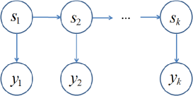
Here we use the HMM to represent the SA process. A graphical illustration of this model is shown in Fig.1, where $k$ denotes the discrete time step, $s$ and $y$ denote the hidden state variable, namely the situation, and the sensor measurement, respectively. In this model, $s$ is a discrete variable, whose value space is defined to be $\mathcal{S}\triangleq\{Situation~{}1,Situation~{}2,\dots,Situation~{}m\}$, where $m\in\mathbb{R}$ representing the total number of situation elements of our interest. Each arrow in Fig.1 indicates a dependence. Therefore, as for this model, the sensor measurement $y$ is straightforwardly dependent on the situation $s$ of current time step, and the situation $s_{k}$ is only dependent on $s_{k-1}$.

Figure 1: Hidden Markov model for SA

Given the HMM model structure as shown above, our task is to calculate the posterior probability density function (pdf) $p(s_{k}|y_{1:k})$, where $y_{1:k}=\{y_{1},y_{2},\dots,y_{k}\}$, $k=1,2,\ldots$. Assume that $p(s_{1}|y_{1})$ is known a priori, then what we are really concerned with is that, given $p(s_{k-1}|y_{1:k-1})$, how to calculate $p(s_{k}|y_{1:k})$, $k=2,3,\ldots.$. Based on Bayes theorem and basic probability calculus, we have

$$p(s_{k}|y_{1:k})=\frac{p(s_{k}|y_{1:k-1})p(y_{k}|s_{k})}{p(y_{k}|y_{1:k-1})},$$ (1)

where

$$p(y_{k}|y_{1:k-1})=\sum_{s_{k}\in\mathcal{S}}p(s_{k}|y_{1:k-1})p(y_{k}|s_{k}),$$ (2)

and

$$p(s_{k}|y_{1:k-1})=\sum_{s_{k-1}\in\mathcal{S}}p(s_{k-1}|y_{1:k-1})p(s_{k}|s_{k-1}).$$ (3)

It is shown that, in order to calculate the posterior $p(s_{k}|y_{1:k})$, it is required to be able to compute the state transition pdf $p(s_{k}|s_{k-1})$ and the likelihood function $p(y_{k}|s_{k})$. Assume that $p(s_{k}|s_{k-1})$ is known a priori, the focus is on the calculation of the likelihood, $p(y_{k}|s_{k})$. As the situation has a higher level semantic meaning, the sensor measurement may not be dependent on it directly. For example, if the sensor produces noisy bearing observations of moving targets monitored within a surveillance region, it would be difficult to build up the straightforward tie between these noisy measurements and the situation. In another word, in that case, there is no easy way to calculate the likelihood $p(y|s)$. We solve the above problem by introducing another hidden variable $x$, which denotes a time-changing state vector including the position and velocity elements of the targets under surveillance. Then we could connect the $y$ with $s$ through $x$, and calculate the likelihood as follows

$$p(y_{k}|s_{k})=\int_{\mathcal{X}}p(x_{k},y_{k}|s_{k})dx_{k}=\int p(y_{k}|x_{k})p(x_{k}|s_{k})dx_{k},$$ (4)

where $\mathcal{X}$ denotes the value space of $x_{k}$. It is shown that, the underlying assumption is that given $x_{k}$, $y_{k}$ is independent with $s_{k}$, which is intuitively reasonable. Under this assumption, to calculate the likelihood $p(y_{k}|s_{k})$, we need to compute $p(x_{k}|s_{k})$, which is determined by the relationship between $s_{k}$ and $x_{k}$. In practice, $p(x|s)$ is usually specified according to the available a priori knowledge coming from domain experts or a knowledge base.

We propose to adopt Gaussian mixture model (GMM) to formulate the a priori knowledge that is used to specify $p(x|s)$. We select the GMM, because it is proved that any continuous pdf can be approximated by a mixture model [18, 19].

For expository purposes, we present an example case of using GMM to model $p(x|s)$ in what follows. Suppose that we are concerned with a threat surveillance problem, and the situation space is $\mathcal{S}=\{\mbox{`danger'},\mbox{`potential danger'},\mbox{`safe'}\}$. The pdf $p(x|s)$ is modeled to be

$$p(x|s=\mbox{`danger'})=\sum_{i=1}^{M_{d}}\omega_{d,i}\mathcal{N}(x|X_{d,i},\Sigma_{d,i}),$$ (5)

$$p(x|s=\mbox{`potential danger'})=\sum_{i=1}^{M_{p}}\omega_{p,i}\mathcal{N}(x|X_{p,i},\Sigma_{p,i}),$$ (6)

$$p(x|s=\mbox{`safe'})=\sum_{i=1}^{M_{sa}}\omega_{sa,i}\mathcal{N}(x|X_{sa,i},\Sigma_{sa,i}),$$ (7)

where $\mathcal{N}(\cdot|X,\Sigma)$ denotes a Gaussian pdf with mean $X$ and covariance $\Sigma$, $M$ denotes the number of mixing components in a mixture pdf, $\omega$ denotes the proportional mass of the mixing components, and the subscripts $d$, $p$ and $sa$ in $\omega$ respectively indicate the situations ‘danger’, ‘potential danger’ and ‘safe’. Assume that some domain or expert knowledge is available. Given such knowledge, the mixture parameters are specified correspondingly. It is noted that rather than manually specifying the model, its parameters could be learnt from labelled historical data. Examples of learning a mixture model to represent the state of moving targets are given in [20, 21].

At this moment, all the details that is required to calculate the posterior, Equation (1), has been completely presented, while another nontrivial issue about computation has to be considered if no analytic close-form solution to $p(y_{k}|s_{k})$ as shown in Equation (4) is existent. We resort to the stochastic simulation techniques to approximate the integral in Equation (4). First we draw random samples, $\hat{x}_{1},\hat{x}_{2},\ldots,\hat{x}_{N}$, from $p(x|s_{k})$. Assume that the sample size $N$ is large enough, the likelihood $p(y_{k}|s_{k})$ can be approximated to be：

$$p(y_{k}|s_{k})\approx\frac{1}{N}\sum_{i=1}^{N}p(y_{k}|\hat{x}_{i}).$$ (8)

According to the large number theory, the accuracy of estimate improves as $N$ tends to infinity.

Note that the above inference process only produces an estimate of the posterior $p(s_{k}|y_{1:k})$, while provides no information about $x_{k}$, as $x$ is marginalized out in Equation (4). In the next subsection, we introduce a novel model, ESSM, based on which both the posterior of $x_{k}$ and that of $s_{k}$ can be estimated in a principled manner.

II-B Mixture based ESSM for SAW

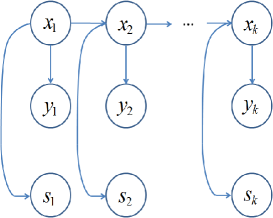
Here we propose a SAW model, ESSM, which is an extension of the state space model that finds applications in tracking problems [22, 23]. The ESSM model is graphically illustrated in Fig.2, where each arrow indicates a dependence and $k$ denotes the discrete time step, the same as for Fig.1. The physical meaning of the hidden variable $x$ could be, e.g., the position and velocity elements of the moving targets of our interest in a surveillance region. The evolution of $x$ is specified by a Markov model $p(x_{k+1}|x_{k})$. The situation $s$, is directly dependent on $x$ of the same time. The only observable variable $y$ denotes the sensor measurements. The same as $s$, $y$ is also dependent on $x$ of the same time. It is worthy to note that the dependence relationship between $s$ and $x$ and that between $y$ and $x$ is totally different. The former is problem specific and is determined by the expert or domain knowledge, while the latter is just determined by the sensor type. The same as in the Sec. II-A, we formulate the knowledge that is needed to model the dependence relationship between $s$ and $x$ based on the GMM.

Figure 2: Extended State Space Model (ESSM) for SA

Given the model structure of ESSM, the posterior $p(s_{k}|y_{1:k})$ can be calculated as follows

$$p(s_{k}|y_{1:k})=\int_{\mathcal{X}}p(x_{k},s_{k}|y_{1:k})dx_{k}=\int_{\mathcal{X}}p(s_{k}|x_{k})p(x_{k}|y_{1:k})dx_{k},$$ (9)

where

$$p(s_{k}|x_{k})=\frac{p(s_{k},x_{k})}{p(x_{k})}=\frac{p(x_{k}|s_{k})p(s_{k})}{\sum_{s\in\mathcal{S}}p(x_{k}|s)p(s)}.$$ (10)

In this model, we assume that $p(s)$ is a uniform distribution, so we have

$$p(s_{k}|x_{k})\varpropto p(x_{k}|s_{k}),$$ (11)

where $p(x|s)$ is modeled by a GMM, in the same way as presented in Sec. II-A.

The posterior pdf of $x$, namely $p(x_{k}|y_{1:k})$, is calculated in a sequential manner as follows. Given $p(x_{k-1}|y_{1:k-1})$, we have

$$p(x_{k}|y_{1:k})=\frac{p(y_{k}|x_{k})\int_{\mathcal{X}}p(x_{k-1}|y_{1:k-1})p(x_{k}|x_{k-1})dx_{k-1}}{p(y_{k}|y_{1:k-1})}.$$ (12)

Suppose that both the state transition prior $p(x_{k}|x_{k-1})$ and the likelihood function $p(y_{k}|x_{k})$ have been defined appropriately, then the state filtering algorithms, such as the Kalman filter and its variants or particle filtering (PF) methods can be used straightforwardly here to calculate Equation (12).

Here we present a PF solution, since the PF can deal with more complex nonlinear and/or non-Gaussian cases. To begin with, let $\{\hat{x}_{k}^{i},w_{k}^{i}\}_{i=1}^{N}$ denote a random measure that approximates $p(x_{k}|y_{1:k})$, which means

$$p(x_{k}|y_{1:k})\simeq\sum_{i=1}^{N}w_{k}^{i}\delta(x_{k}-\hat{x}_{k}^{i}),$$ (13)

where $\delta(\cdot)$ denotes the Dirac delta function.

Assume that at time step $k-1$, a discrete weighted sample set $\{\hat{x}_{k-1}^{i},w_{k-1}^{i}\}_{i=1}^{N}$, which approximates $p(x_{k-1}|y_{1:k-1})$, is available, the task is to get a particle approximation for $p(x_{k}|y_{1:k})$. Employing $p(x_{k}|x_{k-1})$ as the proposal distribution, the importance weights can be determined based on the principle of importance sampling [24]. Specifically, given $\hat{x}_{k-1}^{i}$, draw a random sample $\hat{x}_{k}^{i}$ from the state transition prior, and then calculate the importance weight as follows

$$w_{k}^{i}=\frac{p(y_{k}|\hat{x}_{k}^{i})}{\sum_{i=1}^{N}p(y_{k}|\hat{x}_{k}^{i})},i=1,2,\ldots,N.$$ (14)

Then a Monte Carlo estimate to $p(x_{k}|y_{1:k})$ is available, as shown in Equation (13). A resampling procedure is often used to avoid particle divergence, see details in [23]. Here we present a simple way to implement the PF idea. See alternatives of PF implementations in [23, 25, 26], for example. The convergence properties of the PF methods for nonlinear non-Gaussian state filtering problems have been proved [27, 23, 28].

Now we substitute $p(s_{k}|x_{k})$ and $p(x_{k}|y_{1:k})$ in Equation (9) with Equations (11) and (13), respectively, and then we obtain

$$p(s_{k}|y_{1:k})\varpropto\sum_{i=1}^{N}w_{k}^{i}p(\hat{x}_{k}^{i}|s_{k}).$$ (15)

Because $\sum_{s_{k}\in\mathcal{S}}p(s_{k}|y_{1:k})=1$, we could get a particle approximation of the posterior $p(s_{k}|y_{1:k})$ as follows

$$p(s_{k}|y_{1:k})=\frac{\sum_{i=1}^{N}w_{k}^{i}p(\hat{x}_{k}^{i}|s_{k})}{\sum_{s_{k}\in\mathcal{S}}\sum_{i=1}^{N}w_{k}^{i}p(\hat{x}_{k}^{i}|s_{k})}.$$ (16)

III Simulation results

For expository purposes, we introduce an application of the proposed methods in a toy example. We design a simulation experiment which is similar to the suspicious incoming smuggling vessel case presented in [14]. The objective here is to demonstrate that the proposed mixture idea works. A comparative study of our method with other related methods, for example, MEBN, is certainly interesting but has not yet been performed and is not the intention here.

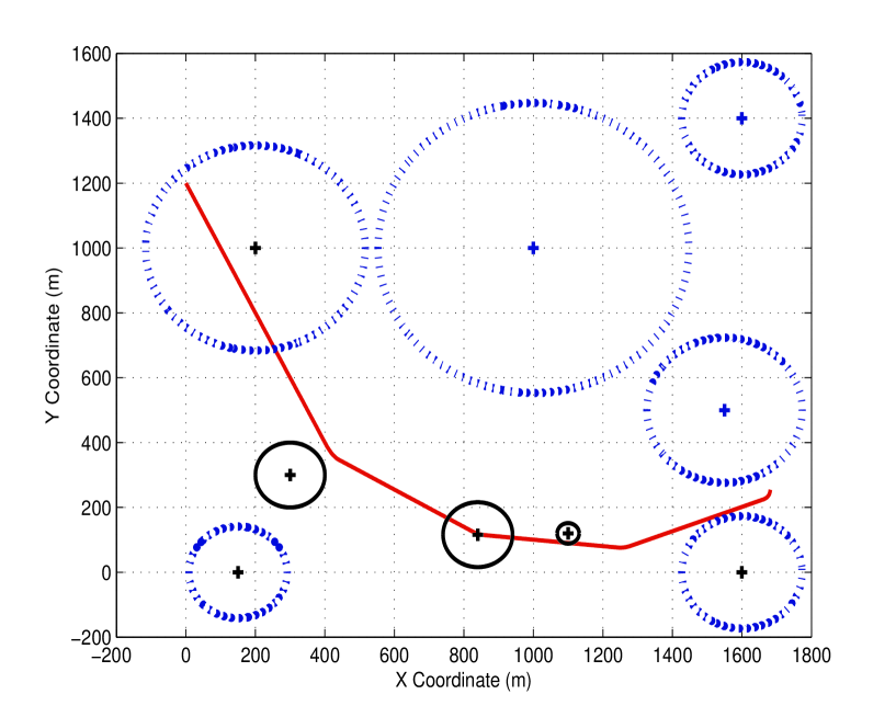
The experiment is about a simulated scenario of threat surveillance. In this scenario, a target moving within a two dimensional surveillance area is monitored by a sensor, which generates noisy bearing and radial distance observations all the time. Within this surveillance area, there are some sensitive regions. Once the target enters into such regions, it indicates that a danger will happen. The task it to design an algorithm that can replace the human operator by automatically percepting and predicting the appearance of the dangerous events in real time. Here the situation parameter space is $\mathcal{S}=\{\mbox{`danger'},\mbox{`potential danger'},\mbox{`safe'}\}$. See Fig.3 for a graphical illustration of the experimental setting, where the solid line denotes the target’s trajectory, and the circles denote the sensitive regions. The target begins moving from the upper left region of the surveillance area.

Figure 3: A graphical description of the simulation settings. The sensor is located at the origin. The target’s trajectory is denoted by the solid lines. The circles drawn with solid and dot lines denote the standard error ellipses associated with the covariance matrices of the mixture pdf conditional on the ‘danger’ situation and those on the ‘safe’ situation, respectively.

In this experimental case, the hidden variable $x$ represents a vector including the two dimensional position and velocity elements of the moving target, i.e.,

$$x_{k}=\left[\textbf{\mbox{x}}_{k}\quad\dot{\textbf{\mbox{x}}_{k}}\quad\textbf{\mbox{y}}_{k}\quad\dot{\textbf{\mbox{y}}_{k}}\right]^{T},$$ (17)

where $(\textbf{\mbox{x}},\textbf{\mbox{y}})$ and $(\dot{\textbf{\mbox{x}}},\dot{\textbf{\mbox{y}}})$ denote the two dimensional position and velocity respectively, and $A^{T}$ denotes the transposition of vector $A$. The target’s movement is characterized by a near constant velocity model as follows

$$\textbf{\mbox{x}}_{k+1}=\textbf{\mbox{f}}_{k}(\textbf{\mbox{x}}_{k},\textbf{\mbox{v}}_{k}),$$ (18)

where

$$\textbf{\mbox{f}}_{k}(\textbf{\mbox{x}}_{k},\textbf{\mbox{v}}_{k})=\textbf{\mbox{F}}\textbf{\mbox{x}}_{k-1}+\textbf{\mbox{v}}_{k},$$ (19)

$\textbf{\mbox{F}}=\left[\begin{array}[]{cc}\textbf{\mbox{F}}_{\textbf{\mbox{s}}}&0\\ 0&\textbf{\mbox{F}}_{\textbf{\mbox{s}}}\end{array}\right],$ $\textbf{\mbox{F}}_{\textbf{\mbox{s}}}=\left[\emph{}\begin{array}[]{cc}1&\mbox{T}\\ 0&1\end{array}\right]$, T denotes the sampling period of the measurements, and v is the process noise, which is zero-mean Gaussian distributed with covariance $\textbf{\mbox{Q}}=\textbf{\mbox{B}}\left[\begin{array}[]{cc}10&0\\ 0&10\end{array}\right]\textbf{\mbox{B}}^{T}$, where

$$\textbf{\mbox{B}}=\left[\begin{array}[]{cc}\mbox{T}&0\\ 0&\mbox{T}\\ \mbox{T}^{2}/2&0\\ 0&\mbox{T}^{2}/2\end{array}\right].$$ (20)

The distribution of the target state $x$ conditional on the situation parameter $s$, i.e., $p(x|s)$, is specified to be

$$p(x|s=\mbox{`danger'})=\sum_{i=1}^{M_{d}}\omega_{d,i}\mathcal{N}(x|X_{d,i},\Sigma_{d,i}),$$ (21)

$$p(x|s=\mbox{`potential danger'})=\sum_{i=1}^{M_{p}}\omega_{p,i}\mathcal{N}(x|X_{p,i},\Sigma_{p,i}),$$ (22)

$$p(x|s=\mbox{`safe'})=\sum_{i=1}^{M_{sa}}\omega_{sa,i}\mathcal{N}(x|X_{sa,i},\Sigma_{sa,i}).$$ (23)

The number of mixing components in $p(x|s=\mbox{`danger'})$ is 3, see Fig.3 for a graphical description of this mixture pdf. The weights of the mixing components in this mixture pdf is fixed to be $1/3$ and the covariance matrix $\Sigma_{d,i}$ is diagonal.

The mixture pdf $p(x|s=\mbox{`potential danger'})$ is set to be the same as $p(x|s=\mbox{`danger'})$, except that the diagonal elements of $\Sigma_{p,i}$ is 10 times bigger than those of $\Sigma_{d,i}$.

The mixing components in $p(x|s=\mbox{`safe'})$ are all dispersive distributions over the surveillance regions excluding the danger and potential danger regions, see Fig.3 for a graphical description of the mixture pdf conditional on the ‘safe’ situation.

In the simulation, the sensor generates noisy measurements including the relative bearing $\theta$ and radial distance $r$ of the target, with respect to the sensor. The sensor noise is Gaussian distributed. The standard errors of the bearing and the radial distance measurements’ distribution are set to be 0.1 degree and 50 meters, respectively.

First we apply the proposed HMM model to this scenario in order to test its effectiveness. The sample size $N$ in Equation (8) is set to be 10,000. The state transition process $p(s_{k+1}|s_{k})$ is determined by the transition table as below

$$\begin{array}[]{cccc}{}\hfil&\mbox{`safe'}&\mbox{`potential danger'}&\mbox{`danger'}\\ \mbox{`safe'}&0.9&0.1&0\\ \mbox{`potential danger'}&0.05&0.9&0.05\\ \mbox{`danger'}&0&0.1&0.9\end{array}.$$ (24)

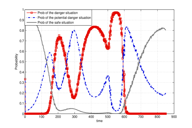
One example run of the HMM based SAW method gives the real time estimate of the posterior, $p(s_{k}|y_{1},\ldots,y_{k})$, as shown in Fig.4. We see that at the beginning, the posterior probabilities of the three situations is the same, then the posterior probability of $s=\mbox{'safe'}$ rises abruptly to be close to 1 and then falls off gradually. The above changes in the output of the approach reflects accurately the initial phase of the experiment when the target has just entered the surveillance region, moving closer to the first sensitive region. From Fig.4, we see that the event $s=\mbox{`potential danger'}$ is most probable after the 130th time step and then the event $s=\mbox{`danger'}$ becomes most probable after about the 180th time step. This is totally consistent with the fact that the target moves closer to the first sensitive region and then enters it during that period. The similar analysis can be performed for the remaining processes of the target’s movement, and it could be found that the output result of the SAW approach is consist with the truth.

It should be noted that, in Fig.3 the target moves through the centre of ‘danger’ region 2 and touches the edge of ‘danger’ region 3, while the maximum probability of ‘danger’ in Fig.4 occurs for region 3. This unexpected observation indicates that the result yielded by the HMM model is not optimal.

Figure 4: The real time situation awareness result by using the proposed HMM model.

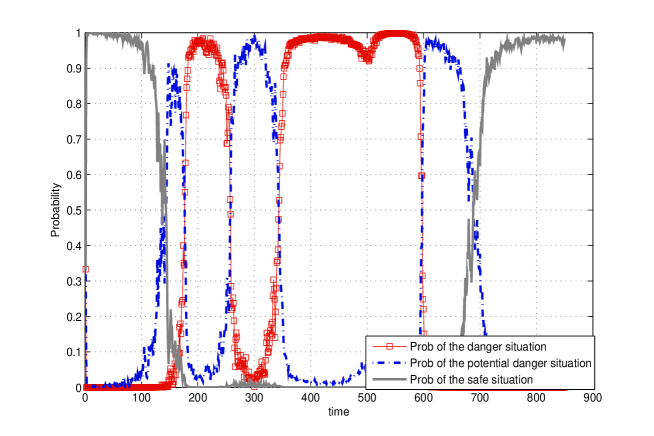
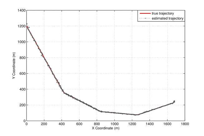
Next we run the ESSM model based SAW approach for this scenario to verify its effectiveness. The particle size used in PF is set to be 5000. The resulting SAW result is shown in Fig.5. Observe that, every time the target enters a sensitive region, the posterior probability of the ‘danger’ situation approaches 1. So, in comparison with the HMM model, the ESSM model is shown to have advantage in leading to more credible detections of the ‘danger’ situation. For other phases of the target’s movement process, the ESSM model always produce expected result that is consistent with the truth. Besides, the ESSM based approach can provide a byproduct, a real time estimate of the target state $x$. The real time estimate of $x_{k}$ outputted from an example run of the ESSM based approach is plotted in Fig.6. As is shown, the estimated target trajectory matches the truth very well.

Figure 5: The real time situation awareness result by using the proposed ESSM model.

Figure 6: The target tracking result given by the PF based on the ESSM model.

Note that the result shown before is not intentionally selected. For both models, we have run the inference algorithm for many times, and the results are very similar as those shown above.

IV Conclusions

In this paper, we studied a statistical modeling approach to do SAW and proposed the idea of using mixture models to formulate the expert/domain knowledge that is required for building the SAW model. We presented two instantiation models, HMM and ESSM, whose implementation is assisted by a GMM based representation of the expert/domain knowledge. The efficiency of the proposed approach is testified by a toy simulation experiment. It is shown that, in comparison with HMM, the ESSM model has advantages in producing more reliable estimation of the situations. Utilization of the ESSM based approach also provides a byproduct, a real time estimate of the target state $x$, which is modeled as a pivot variable that connects the sensor measurement and the situation.

A promising future work consists of a further investigation of the mixture based approach for formulating the expert/domain knowledge in the context of SAW and a theoretical as well as empirical comparison of the proposed approach with the MEBN based methods.

References

- [1] K. Smith and P. Hancock, “The risk space representation of commercial airspace,” in Proc. of the 8th International Symposium on Aviation Psychology, 1995.
- [2] B. Hartman and G. Secrist, “Situational awareness is more than exceptional vision.” Aviation, space, and environmental medicine, vol. 62, no. 11, pp. 1084–1089, 1991.
- [3] M. Vidulich, “Cognitive and performance components of situation awareness: Saint team task one report,” Situation awareness: Papers and annotated bibliography, pp. 17–28, 1994.
- [4] M. R. Endsley, “Measurement of situation awareness in dynamic systems,” Human Factors: The Journal of the Human Factors and Ergonomics Society, vol. 37, no. 1, pp. 65–84, 1995.
- [5] M. L. Hinman, “Some computational approaches for situation assessment and impact assessment,” in Proc. of the 5th International Conf. on Information Fusion, vol. 1. IEEE, 2002, pp. 687–693.
- [6] E. Blasch, “Level 5 (user refinement) issues supporting information fusion management,” in 9th International Conf. on Information Fusion (FUSION). IEEE, 2006, pp. 1–8.
- [7] M. M. Kokar, C. J. Matheus, and K. Baclawski, “Ontology-based situation awareness,” Information fusion, vol. 10, no. 1, pp. 83–98, 2009.
- [8] R. N. Carvalho, P. C. G. Costa, K. B. Laskey, and K.-C. Chang, “Prognos: predictive situational awareness with probabilistic ontologies,” in Proc. of the 13th International Conf. on Information Fusion. IEEE, 2010, pp. 1–8.
- [9] E. Wright, S. Mahoney, K. Laskey, M. Takikawa, and T. Levitt, “Multi-entity bayesian networks for situation assessment,” in Proc. of the 5th International Conf. on Information Fusion, vol. 2. IEEE, 2002, pp. 804–811.
- [10] C. Y. Park, K. B. Laskey, P. C. Costa, and S. Matsumoto, “Multi-entity bayesian networks learning for hybrid variables in situation awareness,” in Proc. of the 16th International Conf. on Information Fusion. IEEE, 2013, pp. 1894–1901.
- [11] S. Das, R. Grey, and P. Gonsalves, “Situation assessment via bayesian belief networks,” in Proc. of the 5th International Conf. on Information Fusion, vol. 1. IEEE, 2002, pp. 664–671.
- [12] Y. Fischer and J. Beyerer, “Modeling of expert knowledge for maritime situation assessment,” International Journal On Advances in Systems and Measurements, vol. 6, no. 3 and 4, pp. 245–259, 2013.
- [13] C. Y. Park, K. B. Laskey, P. C. Costa, and S. Matsumoto, “Predictive situation awareness reference model using multi-entity bayesian networks,” in 17th International Conf. on Information Fusion (FUSION). IEEE, 2014, pp. 1–8.
- [14] Y. Fischer, A. Reiswich, and J. Beyerer, “Modeling and recognizing situations of interest in surveillance applications,” in International Inter-Disciplinary Conf. on Cognitive Methods in Situation Awareness and Decision Support (CogSIMA). IEEE, 2014, pp. 209–215.
- [15] M. Naderpour, J. Lu, and G. Zhang, “An intelligent situation awareness support system for safety-critical environments,” Decision Support Systems, vol. 59, pp. 325–340, 2014.
- [16] R. N. Carvalho, “Probabilistic ontology: Representation and modeling methodology,” Ph.D. dissertation, George Mason University, 2011.
- [17] C. Y. Park, K. B. Laskey, P. C. Costa, and S. Matsumoto, “Multi-entity bayesian networks learning in predictive situation awareness,” DTIC Document, Tech. Rep., 2013.
- [18] A. J. Zeevi and R. Meir, “Density estimation through convex combinations of densities: approximation and estimation bounds,” Neural Networks, vol. 10, no. 1, pp. 99–109, 1997.
- [19] C. M. Bishop et al., Neural networks for pattern recognition. Clarendon press Oxford, 1995.
- [20] R. Laxhammar, “Anomaly detection for sea surveillance,” in 11th International Conf. on Information Fusion (FUSION). IEEE, 2008, pp. 1–8.
- [21] R. O. Lane and K. Copsey, “Track anomaly detection with rhythm of life and bulk activity modeling,” in 15th International Conf. on Information Fusion (FUSION). IEEE, 2012, pp. 24–31.
- [22] J. Durbin and S. J. Koopman, Time series analysis by state space methods. Oxford University Press, 2012, no. 38.
- [23] M. S. Arulampalam, S. Maskell, N. Gordon, and T. Clapp, “A tutorial on particle filters for online nonlinear/non-gaussian bayesian tracking,” IEEE Trans. on Signal Processing, vol. 50, no. 2, pp. 174–188, 2002.
- [24] A. Doucet, S. Godsill, and C. Andrieu, “On sequential monte carlo sampling methods for bayesian filtering,” Statistics and computing, vol. 10, no. 3, pp. 197–208, 2000.
- [25] A. Doucet and A. Johansen, “A tutorial on particle filtering and smoothing: Fifteen years later,” Handbook of Nonlinear Filtering, vol. 12, pp. 656–704, 2009.
- [26] R. Van Der Merwe, A. Doucet, N. De Freitas, and E. Wan, “The unscented particle filter,” in Proc. NIPS, 2000, pp. 584–590.
- [27] D. Crisan and A. Doucet, “A survey of convergence results on particle filtering methods for practitioners,” IEEE Trans. on signal processing, vol. 50, no. 3, pp. 736–746, 2002.
- [28] X.-L. Hu, T. B. Schon, and L. Ljung, “A basic convergence result for particle filtering,” IEEE Trans. on Signal Processing, vol. 56, no. 4, pp. 1337–1348, 2008.