A magnified glance into the Dark Sector: Probing cosmological models with strong lensing in A1689

Abstract

In this paper we constrain four alternative models to the late cosmic acceleration in the Universe: Chevallier-Polarski-Linder (CPL), interacting dark energy (IDE), Ricci holographic dark energy (HDE), and modified polytropic Cardassian (MPC). Strong lensing (SL) images of background galaxies produced by the galaxy cluster Abell $1689$ are used to test these models. To perform this analysis we modify the LENSTOOL lens modeling code. The value added by this probe is compared with other complementary probes: Type Ia supernovae (SNIa), baryon acoustic oscillations (BAO), and cosmic microwave background (CMB). We found that the CPL constraints obtained of the SL data are consistent with those estimated using the other probes. The IDE constraints are consistent with the complementary bounds only if large errors in the SL measurements are considered. The Ricci HDE and MPC constraints are weak but they are similar to the BAO, SNIa and CMB estimations. We also compute the figure-of-merit as a tool to quantify the goodness of fit of the data. Our results suggest that the SL method provides statistically significant constraints on the CPL parameters but weak for those of the other models. Finally, we show that the use of the SL measurements in galaxy clusters is a promising and powerful technique to constrain cosmological models. The advantage of this method is that cosmological parameters are estimated by modelling the SL features for each underlying cosmology. These estimations could be further improved by SL constraints coming from other galaxy clusters.

1. Introduction

The late cosmic acceleration, discovered by the Type IA supernovae (SNIa) observations (Perlmutter et al., 1999; Riess et al., 1998; Schmidt, 1998), is the most intriguing feature of the Universe. What gives origin this phenomenon is a big puzzle in modern cosmology. There are two approaches that could drive the Universe to an accelerated phase: an exotic component dubbed dark energy (DE, Copeland, Sami & Tsujikawa, 2006) and a modification of Einstein’s gravity theory (Tsujikawa, 2010). In the DE scenario, the natural and most simple model is the cosmological constant, $\Lambda$, associated to the vacuum energy, and whose equation of state (EoS) parameter $w$, is equal to $-1$. There are several cosmological observations beyond SNIa data, such as the baryon acoustic oscillations (BAO) and anisotropies of the cosmic microwave background (CMB) radiation, supporting the cosmological constant as the nature of dark energy (Weinberg et al., 2013). Nevertheless, there are theoretical problems associated to the cosmological constant: the fine-tuning problem, i.e., its value is $\sim$120 orders of magnitude below the quantum field theory prediction and the coincidence problem, that is, why the DE density is similar to that of dark matter (DM) today (Weinberg, 1989).

A straightforward way to solve these problems is by considering models where the EoS evolves with time. Among the most studied dynamical DE models are those involving scalar fields, for instance, quintessence (Wetterich, 1988; Peebles & Ratra, 1988; Caldwell, Dave & Steinhardt, 1998; Ratra & Peebles, 1988), phantom (Caldwell, 2002; Chiba, Okabe & Yamaguchi, 2000), quintom (Guo et al., 2005), and k-essence fields (Armendariz-Picon, Mukhanov & Steinhardt, 2000a, b). In addition, there are many models in which the DE EoS is parameterized in terms of the scale factor or redshift (Magaña, Cárdenas & Motta, 2014), for instance, the well-known Chevallier-Polarski-Linder ansatz (CPL, , 2001; Linder, 2003). The possibility of interactions between the DM and DE are also considered by several authors (Bolotin et al., 2015; Caldera-Cabral, Maartens & Urena-Lopez, 2009; Valiviita, 2010). These coupled models could alleviate both the coincidence problem and the tension among different cosmological data (Costa et al., 2014; He, Wang & Abdalla, 2011; Salvatelli et al., 2014; Valiviita & Palmgren, 2015). Other interesting scenarios that have gained interest are the holographic dark energy (HDE) models which are proposed in the context of a fundamental principle of quantum gravity, so called the holographic principle (Cárdenas & Perez, 2010; Cárdenas et al., 2013; ’t Hooft, 1993; Susskind, 1995). Although some HDE models could alleviate the coincidence problem and are in agreement with the cosmological data, they face many issues that must be solved (Cárdenas, Magaña & Villanueva, 2014; del Campo, Cárdenas, Magaña & Villanueva, 2014; Zhang, Li & Noh, 2010).

Thus, there are plenty of models with different theoretical motivations, which are in agreement with some set of observational data and explain the accelerated expansion in the Universe (Li, Li, Wang & Wang, 2013). To discriminate among all these scenarios it is common to put constraints on their parameters using the distance modulus from SNIa, the CMB anisotropies, and BAO (Nesseris & Perivolaropoulos, 2005, 2007; Shi, Huang & Lu, 2012). Many of the current data analysis are performed assuming a fiducial $\Lambda$ cold DM model. Therefore, to improve the cosmological parameter estimation and to avoid biased constraints due to the assumption of a model, it is necessary to acquire high-precision data and to develop new complementary cosmological techniques, such as cosmography, which studies a set of observables of the Universe’s kinematics (see Gruber & Luongo, 2014, and references therein).

Several authors have shown that the strong gravitational effect can be used as a powerful probe to test cosmological models (e.g., Cao, Pan, Biesiada, Godlowski, Zhu, 2012; Chen et al., 2013; Collett et al., 2012; Cárdenas et al., 2013; Jullo et al., 2010; Lubini et al., 2014). Strong lensing (SL) occurs whenever the light rays of a source are strongly deflected by the lens, producing multiples images of the background source. The position of these images depend on the properties of the lens mass distribution. As the Einstein radii also depends on the cosmological model, the SL observations have been used to derive constraints on the DM density parameter, $\Omega_{DM}$, and the EoS for alternative DE models (see for example Biesiada, 2006; Biesiada, Piórkowska & Malec, 2010; Biesiada, Malec, Piórkowska, 2011). In these previous works, the alternative cosmological models are tested by comparing (for the lens systems) the theoretical ratio of the angular diameter distances with an observable. This observable is typically estimated assuming a particular lens model along the standard cosmological paradigm. Nevertheless, the best way should be test the cosmological model by reconstructing the lens model with that underlying new cosmology. A pioneer work using a parametric reconstruction was performed by Jullo et al. (2010) to probe a flat constant $w$CDM model using the SL measurements in the Abell$1689$ (A$1689$) galaxy cluster. They found that the DE EoS estimated with this technique is in agreement with those obtained using CMB and BAO. Recently Lubini et al. (2014) investigated a novel non-parametric SL lens modelling to determine cosmological parameters. They applied this procedure using synthetic lenses and showed that it is possible to infer unbiased constraints from the assumed cosmological parameters. Therefore, SL modeling in galaxy clusters is a powerful and complementary method to put constraints on cosmological parameters (see also D’Aloisio & Natarajan, 2011, and references therein).

In this paper we extend the previous analysis of Jullo et al. (2010) to test four alternative models using the SL measurements of A$1689$ galaxy cluster. We investigate whether this technique is able to put narrow constraints on the dark parameters and the consistency of them with those provided by the SNIa, BAO and CMB data. The paper is organized as follows: in the next section §2 we briefly describe the data used to constrain the cosmological parameters. In section §3 we introduce the framework for a flat Universe and the cosmological models to be tested. In section §4 we define the method to obtain the constrains for each data set We present the results in section §5 and discuss them in section §6. Finally, we give our conclusions in section §7.

2. The data

The following four data sets are used to test the alternative cosmological models: SL measurements in A $1689$ galaxy cluster, SNIa, BAO, and CMB.

SL in A$1689$.- A$1689$ is among the richest clusters given the number density of galaxies in its core, one of the most luminous of galaxy clusters in X-ray wavelengths (Ebeling et al., 1996), it displays an incredible large number of arc systems (see Limousin et al., 2007), and it has been studied using gravitational lensing by several authors (e.g., Limousin et al., 2007, 2013; Diego et al., 2015; Umetsu et al., 2015, and references therein). A$\,1689$ was previously used by Jullo et al. (2010) to simultaneously constrain the cluster mass distribution and DE EoS employing a SL parametric model. We refer the interested reader to that paper, for a detailed description of the methodology to select the final catalog of multiple-image systems used to perform their analysis. In our present work, we are using the same catalog, which consist on 28 images derived from $12$ families with spectroscopic redshift range $1.15<z_{S}<4.86$.

SNIa.- We use the sample presented by Ganeshalingam, Li & Filippenko (2013) consisting on $586$ SNIa in the redshift range $0.01-1.4$ which considers $91$ points of the Lick Observatory Supernova Search (LOSS) sample (Ganeshalingam et al., 2010).

BAOs.- Baryon acoustic oscillation signature is a useful standard ruler to constrain the expansion of the Universe by the distance-redshift measurements from clustering of galaxies with large scale surveys (Blake & Glazebrook, 2003; Seo & Eisenstein, 2003). The BAO measurements considered in our analysis are obtained from the Six-degree-Field Galaxy Survey (6dFGS) BAO data (Beutler et al., 2011), the WiggleZ experiment (Blake et al., 2011), the Sloan Digital Sky Survey (SDSS) Data Release 7 (DR7) BAO distance measurements (Percival et al., 2010), the Baryon Oscillation Spectroscopic Survey (BOSS) SDSS Data Release 9 BAO distance measurements (SDSS DR9, Anderson et al., 2012), and the most recent BAO distance estimations from Data release $11$ (DR11) of the BOSS of SDSS (Delubac et al., 2015).

CMB.- The CMB power spectra is sensitive to the distance to the decoupling epoch, at redshift $z_{*}$, via the locations of peaks and the acoustic oscillations. The CMB measures two distance ratios related to the decoupling epoch: the acoustic scale $l_{A}(z_{*})$, and the shift parameter $R(z_{*})$. A quick way to confront a cosmological model with the CMB data without run a Bayesian global analysis of the power spectra is via the fitting of both distances (Wang & Mukherjee, 2006; Wright, 2007). The cosmological constraints estimated using this method are consistent with those obtained of the full analysis (Komatsu et al., 2009). Moreover, although these distance posterior are computed assuming an underlying cosmology, Li et al. (2008) has demonstrated that these quantities are almost independent on the input DE models. We include CMB information by using the $l_{A}$, $R$, and $z_{*}$ posteriors from the WMAP 9-yr measurements (Hinshaw et al., 2013).

3. Cosmological models

A flat Friedmann-Lemaître-Robertson-Walker (FLRW) Universe with scale factor $a$ and Hubble parameter $H(a)=\dot{a}/a$ is considered. For each cosmological model we use the following components: a source of cosmic acceleration, cold DM and a radiation fluid ($\gamma$, photons and relativistic neutrinos). For this universe, the comoving distance from the observer to redshift $z$ is given by

$$r(z)=\frac{c}{H_{0}}\int_{0}^{z}\frac{dz^{\prime}}{E(z^{\prime})}.$$ (1)

where $E(z)=H(z)/H_{0}$ and $H_{0}=H(0)$. The angular diameter distance for a source at redshift $z$ is

$$D_{A}(z)=\frac{r(z)}{1+z}.$$ (2)

Since we are interested in the ability of SL measurements to constraints the parameters related to the cosmic acceleration and DE, during our analysis we set the Hubble parameter $H_{0}=70\,\mathrm{km\,s^{-1}Mpc^{-1}}$ and $\Omega_{DM0}=0.27$. The current density parameter for radiation is $\Omega_{\gamma 0}=2.469\times 10^{-5}h^{-2}(1+0.2271N_{eff})$, where $h=H_{0}/100\,\mathrm{kms}^{-1}\mathrm{Mpc}^{-1}$ and the number of relativistic species is set to $N_{eff}=3.04$ (Komatsu et al., 2011). At low redshifts, $\Omega_{\gamma}\,(\sim 10^{-5})\ll\Omega_{DM},\Omega_{DE}\,(\sim 1)$, thus we neglect this term when we use the A$1689$ SL measurements, but it is taken into account on the other data sets. The assumption of these fiducial values allows direct model comparisons because each model only has two free parameters related to DE. Bayliss, Sharon & Johnson (2015) produced magnification maps for the Hubble Frontier Fields (HFF) galaxy clusters using priors in $\Omega_{DM0}$ and $H_{0}$. They obtain that varying the input cosmological parameters results in significant differences in the magnification maps. Nevertheless, the influence of the $H_{0}$ and its uncertainty in the lens reconstruction is subdominant because it cancels out when calculating the distance ratio (see Eqs. 1, 2 and 16). On the other hand, the parameter estimation in the SL modelling could be slightly biased due to different choices of $\Omega_{DM0}$. However, this bias is not statistically significative. Thus, for simplicity, we did not take into account the cosmological parameter ($\Omega_{DM0}$, $H_{0}$) uncertainties in the SL lens modelling.

We choose the following alternative cosmological models: Chevallier-Polarski-Linder, interacting dark energy (IDE), Ricci HDE, and modified polytropic Cardassian (MPC). In the following subsections we present the chosen models and the reasons for selecting them.

3.1. Chevallier-Polarski-Linder model

A natural extension to the $\Lambda$CDM scenario which could solve the coincidence problem is to allow the DE EoS to vary with time or redshift via some parametrization. One of the most popular function is the CPL parametrization (, 2001; Linder, 2003) given by

$$w(z)=w_{0}+w_{1}\frac{z}{1+z},$$ (3)

where $w_{0}=w(0)$, $w_{1}=w^{\prime}(0)$ are constants to be fitted by the data. The $E(z)$ function for a FLRW Universe where the DE EoS is parametrized and expressed as

$$E^{2}(z) = \Omega_{\gamma 0}(1+z)^{4}+\Omega_{DM0}(1+z)^{3}+$$ (4)

$$\left(1-\Omega_{DM0}-\Omega_{\gamma 0}\right)f(z),$$

where

$$f(z)=\mathrm{exp}\left(3\int^{z}_{0}\frac{1+w(z)}{1+z}\mathrm{dz}\right).$$ (5)

The substitution of the Eq. (3) in (5) results in:

$$f(z)=(1+z)^{3(1+w_{0}+w_{1})}\exp\left[-\frac{3w_{1}z}{1+z}\right].$$ (6)

Therefore, $E^{2}(z,\Theta)$ for the CPL parametrization reads as

$$E^{2}(z,\Theta)=\Omega_{\gamma 0}(1+z)^{4}+\Omega_{DM0}(1+z)^{3}+$$

$$\left(1-\Omega_{DM0}-\Omega_{\gamma 0}\right)(1+z)^{3(1+w_{0}+w_{1})}\exp\left[-\frac{3w_{1}z}{1+z}\right],\qquad$$ (7)

where $\Theta=(w_{0},w_{1})$ is the vector of the free parameters to be fitted by the data. The CPL parametrization is the fiducial model proposed by the Dark Energy Task Force (DETF) to study the cosmic acceleration (Albrecht et al., 2006). Therefore, the Eq. (7) has been widely used to put constraints on $w_{0}$ and $w{1}$ (see for example Su, Tuo & Cai, 2011; Shi, Huang & Lu, 2012).

3.2. Interacting Dark Energy model

In IDE models there is a relation between the DE energy density ($\rho_{DE}$), and the DM energy density ($\rho_{DM}$) that could alleviate the cosmic coincidence problem. The general approach introduce a $Q$ strength term in the right-side of the continuity equations for the dark components as follows (Amendola, 2000; Caldera-Cabral, Maartens & Urena-Lopez, 2009; , 2005; Dalal, Abazajian, Jenkins & Manohar, 2001; Guo, Ohta & Tsujikawa, 2007; Valiviita, 2010):

$$\dot{\rho_{DM}} + 3H\rho_{DM}=Q,$$

$$\dot{\rho_{DE}} + 3H\left(1+w_{x}\right)\rho_{DE}=-Q,$$ (8)

where $w_{x}$ is the EoS of IDE. There are many choices for the phenomenological energy exchange term $Q$. One of them is to assume $Q$ to be proportional to the Hubble rate, $H$, times either the energy densities or their sum or some other combination of the energy densities. We consider $Q=\delta H\rho_{DM}$, being $\delta$ a constant to be fitted by the data (it is equivalent to $Q=3\delta H\rho_{DM}$ studied by Cao & Liang, 2013; Costa et al., 2014; He, Wang & Abdalla, 2011). A positive $\delta$ describes an energy transfer or a decay of DM to DE and a negative $\delta$ corresponds to an energy transfer from DE to DM. The $E^{2}(z)$ function (see its calculation in Bolotin et al., 2015; Guo, Ohta & Tsujikawa, 2007) for this IDE reads as

$$E^{2}(z,\Theta)=\Omega_{\gamma 0}(1+z)^{4}+$$

$$(1-\Omega_{DM0}-\Omega_{\gamma 0})(1+z)^{3(1+w_{x})}+$$

$$\frac{\Omega_{DM0}}{\delta+3w_{x}}\left[\delta(1+z)^{3(1+w_{x})}+3w_{x}(1+z)^{3-\delta}\right],$$ (9)

where the free parameters to be constrained by the data are $\Theta=(w_{x},\delta)$. The Eq. (9) has been considered in flat (Cao & Liang, 2013; Costa et al., 2014; Guo, Ohta & Tsujikawa, 2007; He, Wang & Abdalla, 2011) and non-flat (Shi, Huang & Lu, 2012) models to put constraints on $w_{x}$ and $\delta$ using several cosmological data.

3.3. Holographic dark energy with Ricci scale and CPL parametrization

Many dark energy models invoke the holographic principle (HP) which states that the number of degrees of freedom of a physical system should be finite and it should scale with its bounding area rather than with its volume (’t Hooft, 1993; Fischler & Susskind, 1998; Susskind, 1995). In HDE it is required that the total energy in a region of size $L$ should not exceed the mass of a black hole of the same size, thus the HDE energy density satisfies $L^{3}\rho_{HDE}\leq M_{p}^{2}L$ (Cohen, Kaplan & Nelson, 1999). This expression imposes a relationship between the ultraviolet (UV, related to the vacuum energy) and infrared (IR, related to large-scale of the Universe) cutoffs. By saturating this inequality, we obtain the following DE energy density

$$\rho_{HDE}=\frac{3c_{H}^{2}M_{p}^{2}}{L^{2}},$$ (10)

where the numerical constant $c_{H}$ is related with the degree of saturation of the previous inequality. Therefore, the DE energy becomes dynamical and the fine-tunning and coincidence problems could be solved. There are several ways to choose the IR cut-off, for example, the Hubble horizon, or the event horizon (del Campo, Fabris, Herrera & Zimdahl, 2011). Here, we consider $L^{2}=6/\mathcal{R}$, where $\mathcal{R}$ is the Ricci scalar defined as $\mathcal{R}=6(2H^{2}+\dot{H})$ (Gao, Wu, Chen & Shen, 2009; del Campo, Fabris, Herrera & Zimdahl, 2011). We also consider that the DM and DE interact with each other obeying Eqs. (8). Following the work by del Campo, Fabris, Herrera & Zimdahl (2011), we parametrize the EoS with the CPL ansatz (3). The $E(z,\Theta)$ parameter (see Appendix A) for this model is the following

$$E^{2}(z,\Theta) = \frac{\left(1+z\right)^{4}}{1+x_{0}+y_{0}}\left(\frac{1+x_{0}}{f}\right)^{2\alpha}\times$$ (11)

$$\left[f+y_{0}\left(\frac{f}{1+x_{0}}\right)^{2\alpha}\right],$$

where $x_{0}=\nicefrac{{\Omega_{DM0}}}{{\Omega_{HDE0}}}$, $y_{0}=\nicefrac{{\Omega_{\gamma 0}}}{{\Omega_{HDE0}}}$, and $\Omega_{HDE0}=1-\Omega_{DM0}-\Omega_{\gamma 0}$. The function $f$ and the exponent $\alpha$ are:

$$f=1+x_{0}+z(1+3w_{1}+x_{0}),$$ (12)

$$\alpha=1-\frac{3(w_{0}+w_{1})}{2(1+3w_{1}+x_{0})}.$$ (13)

The free parameter vector to be fitted by the data is $\Theta=(w_{0},w_{1})$. A similar model without the radiation component was tested by Cárdenas et al. (2013). We present a new analytical solution for the Ricci HDE model with CPL parametrization which includes a relativistic fluid.

3.4. Modified Polytropic Cardassian model

The original Cardassian model was introduced by Freese & Lewis (2002) to explain the accelerated expansion of the universe without DE. Motivated by braneworld theory, this model modifies the Friedmann equation as $H^{2}=8\pi G\rho_{m}/3+B\rho_{m}^{n}$, where $\rho_{m}$ is the total matter density. The second term in the right hand side, known as the Cardassian term, drives the universe to an accelerated phase if the exponent $n$ satisfies $n<2/3$. Gondolo & Freese (2002) introduced a simple generalization of the Cardassian model, the modified polytropic Cardassian, by introducing an additional exponent $q$ (see also Wang, Freese, Gondolo & Lewis, 2003). The modified Friedmann equation with this generalization can be written as

$$H^{2}=\frac{8\pi G}{3}\rho_{m}\left[1+\left(\frac{\rho_{Card}}{\rho_{m}}\right)^{q(1-n)}\right]^{1/q},$$ (14)

where $\rho_{Card}$ is the characteristic energy density with $n<2/3$ and $q>0$. At early times, the universe is expanded according to the canonical Friedmann equation. However, at late times, the Cardassian term dominates driving the universe to an accelerated expansion phase. The equation (14) reduces to the $\Lambda$CDM model for $q=1$ and $n=0$. Introducing a radiation term, the dimensionless $E^{2}(z,\Theta)$ parameter reads as:

$$E^{2}(z,\Theta)=\Omega_{r}(1+z)^{4}+\Omega_{m}(1+z)^{3}\times$$

$$\left[1+\left(\left(\frac{1-\Omega_{r}}{\Omega_{m}}\right)^{q}-1\right)(1+z)^{3q(n-1)}\right]^{1/q},$$ (15)

where the free parameter vector to be fitted by the data is $\Theta=(q,n)$. The flat MPC model (Eq. 15) has been studied by several authors using different data without the radiation component (Feng & Li, 2010) and also with a curvature term (Shi, Huang & Lu, 2012).

4. The method

In this section we explain how the cosmological parameters are estimated for each different observational data set, and we also define the merit functions for each one of them.

4.1. Strong lensing

In the SL regime, the light beams are deflected so strongly that they can result in the observation of several distorted images of a background source. The positions of the multiple images depend significantly on the characteristics of the lens mass distribution. Since the image positions are also related to the angular diameter distance ratios between the lens, source and observer, they retain information about the underlying cosmology. In particular, this dependence of the lensing models on the geometry can be used to derive constraints on the DM density parameter and the DE EoS (see Jullo et al., 2010).

The cosmological models discussed in the section §3 were implemented in LENSTOOL ray-tracing code, which uses a Bayesian Markov chain Monte Carlo (MCMC) method (Jullo et al., 2007). The model fitting is carry out taking into account the cosmological sensitivity of the angular size-redshift relation, when sources are at distinct redshifts (Link & Pierce, 1998). Using this method, the angular diameter distance ratios for $2$ images from different sources defines the ’family ratio’ (see Jullo et al., 2010, for a detailed discussion), for which the constraints on cosmological parameters could be obtained:

$$\Xi(z_{1},z_{s1},z_{s2},\Theta)=\frac{D(z_{1},z_{s1})}{D(0,z_{s1})}\frac{D(0,z_{s2})}{D(z_{1},z_{s2})},$$ (16)

where $\Theta$ is the vector of cosmological parameters to be fitted, $z_{1}$ is the lens redshift, $z_{s1}$ and $z_{s2}$ are the two source redshifts, and $D(z_{1},z_{2})$ is the angular diameter distance, calculated through Eq. (1) and Eq. (2).

We computed the models performing the optimization in the source plane. We solved the lens equation in the source plane because it is computationally more efficient and we checked with some models that source and image plane results were similar. Note that differences can appear for complex clusters with irregular shape (e.g. MACSJ0717.5+3745, Limousin et al., 2012), but this is not the case with Abell 1689. Every lensing mass model (regardless of the DE model) has a total of $21$ free parameters, and consists of two large-scale potentials, a galaxy-scale potential for the central brightest cluster galaxy (BCG), and includes the modeling of $58$ of the brightest cluster galaxies.

For each of the image systems ($12$ families, see §2) with n images, we determine the goodness of fit for a particular set of model parameters defining a $\chi^{2}$:

$$\chi^{2}=\sum_{i=1}^{n}\frac{\left[M(\vec{\beta_{i}}-\langle\vec{\beta}\rangle)\right]^{2}}{\sigma_{i}^{2}},$$ (17)

where $\beta_{i}$ is te source plane position corresponding to image $i$, $\langle\vec{\beta}\rangle$ is the family barycenter, $M$ is the magnification tensor, and $\sigma_{i}$ is the total error (see Jullo et al., 2007). The total $\chi^{2}$ is computed summing over the whole set of families.

4.2. Type Ia Supernovae

The SNIa samples give the distance modulus as a function of redshift $\mu_{obs}(z)$ and its error $\sigma_{\mu}$. Theoretically, the distance modulus is computed as

$$\mu(z)=5\log_{10}[d_{L}(z)/\texttt{Mpc}]+\mu_{0},$$ (18)

where $\mu_{0}$ is a nuisance parameter which depends on the absolute magnitude of a fiducial SN Ia and the Hubble parameter. The $\mu(z)$ is a function of the cosmological model through the luminosity distance (measured in Mpc)

$$d_{L}(z)=(1+z)r(z),$$ (19)

where $r(z)$ is given by Eq. (1). By marginalizing over $\mu_{0}$, we obtain $\chi^{2}_{SNIa}=A-B^{2}/C$, where

$$A = \sum_{i=1}^{586}\frac{[\mu(z_{i})-\mu_{obs}(z_{i})]^{2}}{\sigma_{\mu_{i}}^{2}},$$

$$B = \sum_{i=1}^{586}\frac{\mu(z_{i})-\mu_{obs}(z_{i})}{\sigma_{\mu_{i}}^{2}},$$

$$C = \sum_{i=1}^{586}\frac{1}{\sigma_{\mu_{i}}^{2}}.$$ (20)

The SNIa constraints can be estimated by minimizing the $\chi^{2}_{SNIa}$.

4.3. BAOs measurements

The 6dFGS BAO estimated the distance ratio $d_{z}=0.336\pm 0.015$ at $z=0.106$ (Beutler et al., 2011), where

$$d_{z}=\frac{r_{s}(z_{d})}{D_{V}(z)}.$$ (21)

The comoving sound horizon, $r_{s}(z)$, is defined as

$$r_{s}(z)=c\int_{z}^{\infty}\frac{c_{s}(z^{\prime})}{H(z^{\prime})}dz^{\prime},$$ (22)

where the sound speed is $c_{s}(z)=1/\sqrt{3(1+\bar{R_{b}}/(1+z)}$, with $\bar{R_{b}}=31500\,\Omega_{b}h^{2}(T_{CMB}/2.7\,\mbox{K})^{-4}$, $\Omega_{b}$ is baryonic density parameter, and $T_{CMB}$ is the CMB temperature ($2.726$K for WMAP 9-yr, Hinshaw et al., 2013). The distance scale $D_{V}$ is defined as

$$D_{V}(z)=\frac{1}{H_{0}}\left[(1+z)^{2}D_{A}(z)^{2}\frac{cz}{E(z)}\right]^{1/3},$$ (23)

where $D_{A}(z)$ is the angular diameter distance given by Eq. (2).

The redshift $z_{d}$ at the baryon drag epoch is fitted with the formula proposed by Eisenstein & Hu (1998),

$$z_{d}=\frac{1291(\Omega_{m}h^{2})^{0.251}}{1+0.659\,(\Omega_{m}h^{2})^{0.828}}[1+b_{1}(\Omega_{b}h^{2})^{b_{2}}],$$ (24)

where

$$b_{1} = 0.313\left(\Omega_{m}\,h^{2}\right)^{-0.419}\left[1+0.607\left(\Omega_{m}\,h^{2}\right)^{0.674}\right],$$ (25)

$$b_{2} = 0.238\left(\Omega_{m}\,h^{2}\right)^{0.223}.$$ (26)

Therefore, the $\chi^{2}$ for the BAO data point from 6dFGS is

$$\chi^{2}_{\scriptscriptstyle 6dFGS}=\left(\frac{d_{z}-0.336}{0.015}\right)^{2}.$$ (27)

The WiggleZ BAO estimated three points for the acoustic parameter $A(z)$ (Eisenstein et al., 2005)

$$A(z)=\frac{D_{V}(z)\sqrt{\Omega_{m}H_{0}^{2}}}{cz}.$$ (28)

The observational data are $\bar{A}_{obs}=(0.474,0.442,0.424)$ for the effective redshifts $z=0.44,0.6$ and 0.73 respectively.

Thus, the $\chi^{2}$ for the WiggleZ BAO data is given by

$$\chi^{2}_{\scriptscriptstyle WiggleZ}=(\bar{A}_{obs}-\bar{A}_{th})C_{\scriptscriptstyle WiggleZ}^{-1}(\bar{A}_{obs}-\bar{A}_{th})^{T},$$ (29)

where $\bar{A}_{th}$ denotes the theoretical value for the acoustic parameter $A(z)$ and $\bar{A}_{obs}$ the observed one. The inverse covariance $C_{\scriptscriptstyle WiggleZ}^{-1}$ is given by

$$C_{\scriptscriptstyle WiggleZ}^{-1}=\left(\begin{array}[]{ccc}1040.3&-807.5&336.8\\ -807.5&3720.3&-1551.9\\ 336.8&-1551.9&2914.9\end{array}\right).$$ (30)

Similarly, for the SDSS DR7 BAO distance measurements, the $\chi^{2}$ can be expressed as

$$\chi^{2}_{\scriptscriptstyle DR7}=(\bar{d_{z}}_{obs}-\bar{d_{z}}_{th})C_{\scriptscriptstyle DR7}^{-1}(\bar{d_{z}}_{obs}-\bar{d_{z}}_{th})^{T},$$ (31)

where $\bar{d_{z}}_{obs}=(0.190195,0.1097)$ are the data at $z=0.2$, and $0.35$ respectively (Percival et al., 2010). Here $\bar{d_{z}}_{th}$ denotes the theoretical distance ratio given by Eq. (21). The inverse covariance matrix $C_{\scriptscriptstyle DR7}^{-1}$ reads as

$$C_{\scriptscriptstyle DR7}^{-1}=\left(\begin{array}[]{cc}30124&-17227\\ -17227&86977\end{array}\right).$$ (32)

The SDSS DR9 estimated the distance ratio $d_{z}=0.0732\pm 0.0012$ at $z=0.57$ (Anderson et al., 2012). For this BAO data point, the $\chi^{2}$ function is given by

$$\chi^{2}_{\scriptscriptstyle DR9}=\left(\frac{d_{z}-0.0732}{0.0012}\right)^{2}.$$ (33)

The most recent measured position of the BAO peak from SDSS DR11 determine $D_{H}/r_{d}=9.18\pm 0.28$ at $z=2.34$, where $D_{H}=c/H$ and $r_{d}=r_{s}(z_{d})$ (Delubac et al., 2015). We compute the $\chi^{2}$ for this point as

$$\chi^{2}_{\scriptscriptstyle DR11}=\left(\frac{D_{H}/r_{d}-9.18}{0.28}\right)^{2}.$$ (34)

Therefore, the total $\chi^{2}$ function for the BAO measurements is

$$\chi^{2}_{BAO}=\chi^{2}_{\scriptscriptstyle 6dFGS}+\chi^{2}_{\scriptscriptstyle WiggleZ}+\chi^{2}_{\scriptscriptstyle DR7}+\chi^{2}_{\scriptscriptstyle DR9}+\chi^{2}_{\scriptscriptstyle DR11}.$$ (35)

The BAO constraints can be estimated by minimizing the Eq. (35).

4.4. CMB

We use the following WMAP 9-yr distance posterior (Hinshaw et al., 2013) for a flat $\Lambda$CDM Universe: $l_{A^{obs}}=302.40$, $R^{obs}=1.7246$, $z_{*}^{obs}=1090.88$, and the inverse covariance matrix

$$C_{WMAP9}^{-1}=\left(\begin{array}[]{ccc}3.182&18.253&-1.429\\ 18.253&11887.879&-193.808\\ -1.429&-193.808&4.556\end{array}\right).$$ (36)

The acoustic scale is defined as

$$l_{A}=\frac{\pi r(z_{*})}{r_{s}(z_{*})},$$ (37)

and the redshift of decoupling $z_{*}$ is given by (Hu & Sugiyama, 1996),

$$z_{*}=1048[1+0.00124(\Omega_{b}h^{2})^{-0.738}][1+g_{1}(\Omega_{m}h^{2})^{g_{2}}],$$ (38)

$$g_{1}=\frac{0.0783(\Omega_{b}h^{2})^{-0.238}}{1+39.5(\Omega_{b}h^{2})^{0.763}},g_{2}=\frac{0.560}{1+21.1(\Omega_{b}h^{2})^{1.81}}.$$ (39)

The shift parameter is defined as (Bond, Efstathiou & Tegmark, 1997)

$$R=\frac{\sqrt{\Omega_{m}H_{0}^{2}}}{c}r(z_{*}).$$ (40)

Thus, the CMB constraints can be estimated by minimizing

$$\chi^{2}_{CMB}=X^{T}C_{CMB}^{-1}X,$$ (41)

where

$$X=\left(\begin{array}[]{c}l_{A}^{th}-l_{A}^{obs}\\ R^{th}-R^{obs}\\ z_{*}^{th}-z_{*}^{obs}\end{array}\right),$$ (42)

and the superscripts $th$ and $obs$ refer to the theoretical and observational values respectively.

5. Results

The parameters of the alternative models are determined by minimizing the $\chi^{2}$ function for each data set. For all models, first we calculate the minimum values using the SL data with the priors described by Jullo et al. (2010). Then, we estimate the constraints using the SNIa, BAO, and CMB, comparing the different data sets. Furthermore we could use a refined $\chi^{2}_{min}$ criteria, for instance, the Akaike information criterion (AIC), and the Bayesian information criterion (BIC), to discern which model is prefered by the data. However, since all the tested models have only two free parameters, the information provided by the $\chi^{2}_{min}$ values is sufficient and AIC and BIC criteria does not provide further information.

CPL .- The best fits on the EoS parameters $w_{0}$ and $w_{1}$ for the CPL model and the estimated $\chi^{2}$ using each data set are listed in Table 1. Note that the limits derived for the A$1689$ SL data are in tension with those obtained with the SNIa, BAO, and 9yr-WMAP data. Actually, the A$1689$ constraint on $w_{0}$ is positive implying no cosmic acceleration. The Fig. 1 shows the marginalized contours at $1\sigma$, $2\sigma$ and $3\sigma$ for the CPL parameters. The inset shows the region where the different contours overlap.

Table 1CPL model

Data set	$\chi^{2}_{min}$	FoM	$w_{0}$	$w_{1}$
A$1689$	$264.9$	$8.20$	$0.43\pm 0.48$	$-6.45^{+3.60}_{-0.36}$
SNIa	$574.13$	$24.41$	$-0.82\pm 0.14$	$-1.51\pm 0.91$
BAO	$3.77$	$7.89$	$-0.94\pm 0.26$	$-1.55\pm 1.72$
CMB	$0.363$	$21.54$	$-0.59\pm 0.58$	$-1.38\pm 2.36$

Note. — Best fits for the $w_{0}$ and $w_{1}$ CPL parameters estimated from the SL measurements in A$1689$, SNIa, BAO and CMB.

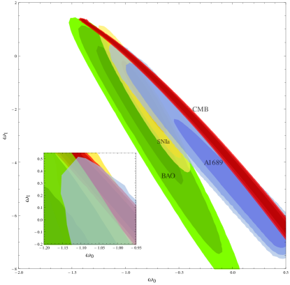
Figure 1.— The $1\sigma$, $2\sigma$ and $3\sigma$ contours of the CPL model parameters $w_{0}$ and $w_{1}$ obtained from different data sets: Abell 1689 (blue), SNIa (yellow), CMB (red) and BAO (green). The inset shows the region where the contours overlap

IDE .- We have carried out two different analysis using the SL data: the first one, A$1689$M1, with the (astrometric) errors in the image positions of the systems previously used by Jullo et al. (2010) (also used in the other three models of this paper) and the other, A$1689$M2, in which we have set the errors as five times the values of the fiducial model, i.e., five times the errors in model A$1689$M1, so that we obtain a reduced $\chi^{2}\simeq 1$. These large errors take into account other possible sources of uncertainties in the SL measurements such as systematic errors due to the complexities in the mass distribution and the line-of-sight structures (e.g. D’Aloisio & Natarajan, 2011; Jullo et al., 2010). In §6.2 we will resume the discussion again.

The best fits on the $w_{x}$ and $\delta$ parameters for both runs of the IDE model and the estimated $\chi^{2}$ using each data set are listed in Table 2. Note that A$1689$M1 constraints on $w_{x}$ and $\delta$ are in disagreement with the estimations of the other cosmological tests. In the second analysis, considering larger errors on the SL data, we obtain that the best fit on $w_{x}$ is in agreement at $1\sigma$ with the others data. The Fig. 2 shows the marginalized $1\sigma$, $2\sigma$ and $3\sigma$ confidence contours in the plane $w_{x}-\delta$ for each data set. The inset shows the region where the A$1689$M2 contours overlap with SNIa, BAO, and CMB contours.

Table 2IDE model

Data set	$\chi^{2}_{min}$	FoM	$w_{x}$	$\delta$
A$1689\mbox{M}1$	$256.7$	$127.063$	$-0.32\pm 0.07$	$-2.0^{+0.30}_{-0.0}$
A$1689\mbox{M}2$	$25.9$	$4.55$	$-1.53\pm 0.42$	$-0.21\pm 0.80$
SNIa	$574.95$	$38.76$	$-0.95\pm 0.08$	$0.77\pm 0.69$
BAO	$4.61$	$1060.52$	$-1.10\pm 0.13$	$-0.0093\pm 0.014$
CMB	$0.081$	$18488.1$	$-0.97\pm 0.02$	$-0.0017\pm 0.003$

Note. — Best fits for the $w_{x}$ and $\delta$ IDE parameters estimated from the SL measurements in A$1689$, SNIa, BAO and CMB.

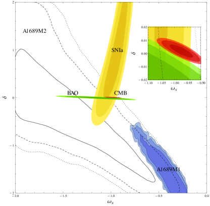
Figure 2.— The $1\sigma$, $2\sigma$ and $3\sigma$ contours of the IDE model parameters $\delta$ and $w_{x}$ obtained from different data sets: A$1689$M1 (blue), SNIa (yellow), CMB (red) and BAO (green). The contours for the run A$1689$M2 considering large errors are: $1\sigma$ in solid line, $2\sigma$, dashed line, and $3\sigma$ dotted line. The inset shows the region where the of SNIa, BAO and CMB contours overlap with those of the A$1689$M2 analysis.

Ricci HDE .- The The best fits on $w_{0}$ and $w_{1}$ parameters and the $\chi^{2}$ obtained using each data set are shown in Table 3. Note that A$1689$ best fits are consistent with those of the CMB data. Nevertheless, there is a tension between these values and the BAO and SNIa constraints. Figure 3 shows the marginalized confidence contours at $1\sigma$, $2\sigma$, and $3\sigma$ in the parameters space $w_{0}$-$w_{1}$. The inset shows the region where the contours overlap.

Table 3HDE model

Data set	$\chi^{2}_{min}$	FoM	$w_{0}$	$w_{1}$
A$1689$	$279.82$	$24.85$	$-1.60^{+0.13}_{-0.0}$	$1.97^{+0.01}_{-0.66}$
SNIa	$575.135$	$153.89$	$-0.96\pm 0.10$	$0.21\pm 0.22$
BAO	$5.79$	$241.52$	$-2.03\pm 0.21$	$2.10\pm 0.21$
CMB	$0.081$	$14725.7$	$-1.48\pm 0.01$	$1.51\pm 0.01$

Note. — Best fits for the $w_{0}$ and $w_{1}$ Ricci HDE parameters estimated from the SL measurements in A$1689$, SNIa, BAO and CMB.

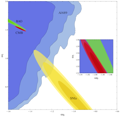
Figure 3.— The $1\sigma$, $2\sigma$ and $3\sigma$ contours of the Ricci HDE model parameters $w_{0}$ and $w_{1}$ obtained from different data sets: Abell1689 (blue), SNIa (yellow), CMB (red) and BAO (green). The inset shows the region where the contours overlap.

MPC .- The best fits on the $q$ and $n$ parameters and the estimated $\chi^{2}$ using each data set are listed in Table 4. Note that the A$1689$ constraints on $q$ and $n$ are consistent with the limits given by CMB data. Although, these SL and CMB best fits are in tension with the estimations obtained with SNIa and BAO observations, the errors for the $q$ parameter are statistically larger, thus the constraints for each data are consistent at $1\sigma$. Figure 4 shows the marginalized confidence contours at $1\sigma$, $2\sigma$, and $3\sigma$ in the parameters space $q$-$n$. An interesting aspect of the SL contours is that the A$1689$ data provided two $1\sigma$ regions. The inset shows a region where the different contours overlap.

Table 4MPC model

Data set	$\chi^{2}_{min}$	FoM	$q$	$n$
A$1689$	$266.7$	$2.54$	$5.2\pm 2.25$	$0.41\pm 0.25$
SNIa	$574.52$	$18.69$	$3.20\pm 2.19$	$0.32\pm 0.08$
BAO	$3.59$	$7.97$	$3.29\pm 3.30$	$0.26\pm 0.13$
CMB	$0.363$	$37.63$	$4.52\pm 3.27$	$0.49\pm 0.05$

Note. — Best fits for the $q$ and $n$ Cardassian parameters estimated from the SL measurements in A$1689$, SNIa, BAO and CMB.

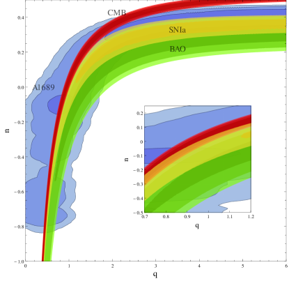
Figure 4.— The $1\sigma$, $2\sigma$ and $3\sigma$ contours of the MPC model parameters $q$ and $n$ obtained from different data sets: A$1689$ (blue), SNIa (yellow), CMB (red) and BAO (green). The inset shows the region where the contours overlap.

6. Discussion

6.1. CPL

By combining WMAP-9yr data, the measurements of CMB from Atacama Cosmology Telescope (ACT) and the South Pole Telescope (SPT), BAO points, and $H_{0}$ measurements, Hinshaw et al. (2013) estimated $w_{0}=-1.17^{+0.13}_{-0.12}$, $w_{1}=0.35^{+0.50}_{-0.49}$. These values are in concordance at $1\sigma$ within our limits although there is a significative tension in the constraints on $w_{1}$. Furthermore, the SL estimations are consistent with $w_{0}=-1.04^{+0.72}_{-0.69}$, $w_{1}<1.32$ and the approximated range $-1.2<w_{0}<-0.5$, $-1.8<w_{1}<0.2$ obtained by Planck collaboration (2013, 2015) respectively. Note that the SL contours (see Fig. 1) are analogous to those obtained with the other data. The overlapped region suggests the cutoffs $w_{0}\approx-1.05$ and $w_{1}\sim 0.2$, which is consistent with the cosmological constant. It is worthy to mention that the CPL contours, using the different data sets, are similar to those computed by Planck collaboration (2015).

6.2. IDE

For the SL, BAO, and CMB data the $\delta$ constraints are negative suggesting an energy transfer from DM to DE opposite to the SNIa constraint. Moreover, there is a tension with the contraints provided by the BAO and CMB data which favor no evidence of dark interactions. The Fig. 2 shows that the contours obtained from the run A$1689$M1 do not overlap with the plots computed using the other data. Nevertheless, the contours derived of the analysis A$1689$M2 are consistent and orthogonal with those of SNIa, BAO and CMB data. These contours, computed assuming the aforementioned large errors in the image position of the SL systems, indicates that it is necessary to take into account all the sources of errors (including systematic errors) in the SL models to avoid severe biases in the calculations of DE constraints (D’Aloisio & Natarajan, 2011). Furthermore, several authors have shown that the line-of-sight structure is a significant source of uncertainty in the SL mass modelling, and consequently, in the observed image positions (Bayliss et al., 2014; Host, 2012; Jaroszynski & Kostrzewa-Rutkowska, 2014; McCully et al., 2014; Zitrin et al., 2015). While our assumed errors could be slightly overestimated (see e.g. Zitrin et al., 2015), D’Aloisio & Natarajan (2011) showed that the observational errors (in the case of space-based imaging) are typically an order of magnitude lower than potential modelling errors. Thus, a realistic SL model should take these uncertainties into account by using large errors in the position of multiple images.

Although the data from A$1689$M2 give weak constraints on the IDE parameters, they provide significant evidence of interactions between the DM and DE. The overlapped region of the Fig. 2 suggests the cutoffs $w_{x}\approx-1$ and $-0.005<\delta<0.005$, which is consistent with the cosmological constant and no interactions in the dark sector. Similar constraints on $\delta$ was also obtained by He, Wang & Abdalla (2011) using the WMAP seven-year data and others cosmological observations (see also the consistency with the bounds estimated by Cao & Liang, 2013). In a recent paper by Costa et al. (2014), the authors put constraints on this IDE model using Planck data in combination with SNIa, BAO, and Hubble parameter measurements. They found $w_{x}\approx-1.65$ for CMB data alone and $w_{x}\approx-1.25$ from the joint analysis. In addition, they found slightly evidence of energy transfer from DE to DM ($\delta\sim 0.006$).

6.3. Ricci HDE

Recently, Cárdenas et al. (2013) tested this model without the radiation fluid performing a joint analysis of SL, BAO, SNIa, and $H(z)$ data (see also del Campo, Fabris, Herrera & Zimdahl, 2011). They found $w_{0}=-1.27^{+0.12}_{-0.13}$ and $w_{1}=0.99^{+0.30}_{-0.26}$. These values are consistent at $2\sigma$ with our constraints obtained of A$1689$ SL measurements. The Ricci HDE confidence contours (see Figure 3) show that SL data produce weaker constraints on $w_{0}$ and $w_{1}$. Moreover, the $1\sigma$ SL contour overlap with the CMB bounds and only at $2\sigma$, and $3\sigma$ for the BAO and SNIa data. It is worthy to note that the SNIa contours are only overlap with those derived of the SL probe. Several authors have pointed out that this tension between the SNIa constraints together with those of BAO and CMB tests could be due to the choice of priors on the DM density parameter, statistical and systematic errors in the data sets, the choice of different SNIa light-curve fitters, etc (see for example Escamilla-Rivera et al., 2011; Gong, Wang, & Cai, 2010; Lazkoz, Nesseris & Perivolaropoulos, 2008; Li, Wu & Yu, 2011; Magaña, Cárdenas & Motta, 2014; Nesseris & Perivolaropoulos, 2005; Perivolaropoulos & Shafieloo, 2009). The tension of the Ricci HDE constraints derived from several data sets will be further investigated in a forthcoming work.

6.4. MPC

Several authors have tested the MPC model using different data sets. For instance, the Cosmic All-Sky Survey (CLASS) lensing sample have been used by Alcaniz, Dev & Jain (2005) to obtain the constraints $q=0.05$ and $n=-2.32$ which are in tension with our SL fits. Wang & Wu (2009) estimated, using SNIa, BAO, CMB, Hubble parameter measurements and the gas mass fraction in galaxy clusters, $q=0.824^{+0.750}_{-0.622}$, and $n=-0.091^{+0.331}_{-1.908}$ which are in agreement with our confidence contours (see Figure 4). In addition, our limits are similar at $1\sigma$ to $q=0.480^{+2.020}_{-0.080}$, $n=-0.600^{+0.980}_{-0.450}$ computed by Feng & Li (2010) using the combination of SNIa (Constitution sample), BAO, and 5-yrs WMAP data. By combining SNIa, BAO, CMB and gamma-ray burst data, Liang, Wu & Zhu (2011) found $q=0.76^{+0.36}_{-0.58}$ and $n=-0.16^{+0.25}_{-3.26}$ in accordance with one of the $1\sigma$ SL contour as well as those of CMB, and SNIa. Recently, Li, Wu & Yu (2011) use different SNIa samples together with BAO and CMB data to put the constraints $q=1.098^{+1.015}_{-0.465}$ and $n=0.014^{+0.364}_{-0.964}$ which are consistent with our limits at $1\sigma$. Note that the SL contours are similar in shape and orientation to those obtained with the other data. In addition, our confidence contours are similar to those computed by Liang, Wu & Zhu (2011); Li, Wu & Yu (2011); Wang & Wu (2009) The overlapped region (see inset of Figure 4) suggests the cutoffs $0.45<q<1.05$ and $-0.8<n<0.05$. The weak constraints on the MPC parameters obtained with the different data sets do not provide strong evidence of modifications to the Friedmann equations, hence of cosmic acceleration without DE.

6.5. Merit of the SL method

As we showed and discussed above, the SL technique provides complementary constraints to the standard cosmological probes. It is important to stress that the determination of which cosmological model is favored by the data, mainly by the SL measurements, is far from the scope of the present work (the current data do not allow us to undertake such detailed analysis). Nevertheless, by considering standard errors in the SL data, the IDE model gives the lowest value of the SL $\chi^{2}_{min}$, therefore it is the favored by the A$1668$ SL measurements. However, as discussed in §6.2, the SL constraints for this IDE model are in disagreement with the those of SNIa, BAO, and CMB. The CPL model is the second one preferred by the SL data.

Another useful tool to quantify the ability of each observational data to constrain the cosmological parameters is considering the Figure-of-Merit (FoM, Albrecht et al., 2006; Su, Tuo & Cai, 2011; Wang, 2008). The DETF defined the FoM for the CPL model as the inverse of the area enclosed by the 95% confidence level contour of $(w0,wa)$ (Albrecht et al., 2006). Wang (2008) introduced a more general definition given by

$$\mbox{FoM}=\frac{1}{\sqrt{\det\mbox{Cov}(f1,f2,f3,...)}},$$ (43)

where $\mbox{Cov}(f1,f2,f3,...)$ is the covariance matrix of the cosmological parameters $f_{i}$. Larger FoM means stronger constraints on the parameters since it corresponds to a smaller error ellipse. We have computed the FoM of the cosmological models for each data set. The results are shown in the third column of the Tables 1-4. For a more intuitive comparision, we show in Figure 5 the values of the FoM for each model using each data set. Note that for the CPL model, the SL probe gives slightly more stringent constraints than the BAO test. In the case of A$1689$M1, although the SL FoM is $\sim 3.3$ times greater than that SNIa, the constraints obtained from this lens model are inconsistent with the others tests. For the A$1689$M2 analysis with large errors on the SL measurements, the SL FoM has the lowest value, indicating that this technique provides weak constraints on the IDE parameters. The FoMs for the HDE and MPC models from the A$1689$ data are also the lowest when compared with the other cosmological probes. Although it is very difficult to compare the SL FoM for different models, our computations suggest that the SL technique provides statistically significant constraints on the CPL parameters but a weak for the other models.

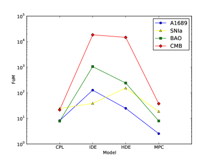
Figure 5.— FoM for each model using A$1689$, SNIa, BAO and CMB data.

In spite of the general low FoM for the SL probe compared with the other data sets, it is important to remark that we only use the measurements of one galaxy cluster, namely, A$1689$. To improve the SL constraints on the parameters of the alternative cosmological models we need to consider the SL measurements in other galaxy clusters. This work is a first test of the capability of this technique to constrain unusual cosmological models. D’Aloisio & Natarajan (2011) showed that using the data from 10 simulated galaxy clusters, each one with 20 multiply imaged families, the estimated constraints on the parameters of the $w$CDM and CPL models are improved. We plan to extend this analysis using the coming data from future surveys such as The Frontier Fields (FF) program of the Hubble space telescope. In addition, it is crucial that future efforts also take into account for additional uncertainties in the lens modelling due to line-of-sight structure and other systematic errors (Bayliss et al., 2014; Host, 2012; Jaroszynski & Kostrzewa-Rutkowska, 2014; McCully et al., 2014). Finally, it is important to point out that the cosmological constraints obtained in this work could be affected by other unknown systematics (Bayliss et al., 2014; Bayliss, Sharon & Johnson, 2015; Zitrin et al., 2015) such as the SL modelling technique.

7. Conclusions

One of the main goals of observational cosmology is to elucidate what gives origin to the late cosmic acceleration in the Universe. A wide set of theoretical models have been proposed to explain this cosmic feature (Li, Li, Wang & Wang, 2013) and need to be tested with observational data (Albrecht et al., 2006; Lazkoz, Nesseris & Perivolaropoulos, 2008; Nesseris & Perivolaropoulos, 2005, 2007). In this paper, we put constraints on four alternative cosmological models: Chevallier-Polarski-Linder parametrization, interacting dark energy, Ricci holographic dark energy and modified polytropic Cardassian. We mainly focus on a powerful and not fully exploited technique which uses the strong lensing measurements in A$\,1689$ galaxy cluster (Jullo et al., 2010). The advantage of the method presented here is that the cosmological parameters are estimated by modelling the SL features for each underlying cosmology. Additionally, we use the SNIa, BAO and CMB signal as complementary probes. We have shown that for the CPL model the SL method provide constraints in agreement with those estimated with the other probes. We performed two analysis for the IDE model, one with standard errors in the SL measurements and the other with larger errors to takes into account other sources of uncertainties (Bayliss et al., 2014; D’Aloisio & Natarajan, 2011; Host, 2012; Jaroszynski & Kostrzewa-Rutkowska, 2014; McCully et al., 2014; Zitrin et al., 2015). We found that the limits on the IDE parameters derived of the standad error analysis are in disagreement with the standard tests. Moreover, the confidence contours do not overlap with those of SNIa, BAO, and CMB. Nevertheless, if larger errors in the SL measurements are considered, the SL estimations are consistent with the constraints obtained from other probes. Therefore, underestimating the total error can lead to erroneous constraints on the parameters of the IDE model. For the Ricci HDE, the SL data give weak constraints on the DE EoS parameters. In addition, we also found a tension between the bounds obtained from SNIa, BAO and CMB data. Finally, the estimations for the MPC parameters using the SL test are similar to the SNIa, BAO, and CMB contraints. We calculate also the figure-of-merits to quantify the goodness of fitting using the different data. We found that in general the SL constraints are weak when compared with other tests. Also, contours not always overlap with each other, suggesting some systematic errors in the models of the observables that remain to be investigated. Nevertheless, it is worthy to note that we use only data from one galaxy cluster. The cosmological constraints could be improved if more SL data are used (D’Aloisio & Natarajan, 2011). Our results show that this is a powerful technique that will be used in the future, when more data are available, in particular those for the HFF clusters.

Appendix A The $E(z)$ analytical solution for the Ricci HDE model with a radiation component

In this paper we have revisited the HDE with Ricci scale model presented by del Campo, Fabris, Herrera & Zimdahl (2011) and Cárdenas et al. (2013) but we have taken into account the radiation component. We consider a flat FLRW universe with DM, HDE, and radiation. By assuming the possibility of interaction between the dark components, the dynamics of this universe is governed by the system

$$H^{2} =\frac{8\pi G}{3}\left(\rho_{DM}+\rho_{HDE}+\rho_{r}\right),$$ (A1a)

$$\dot{\rho_{DM}} +3H\rho_{DM}=Q,$$ (A1b)

$$\dot{\rho_{HDE}} +3H(1+\omega)\rho_{HDE}=-Q,$$ (A1c)

$$\dot{\rho_{\gamma}} +4H\rho_{\gamma}=0,$$ (A1d)

such that the total energy, $\rho=\rho_{DM}+\rho_{HDE}+\rho_{\gamma}$, is conserved. Here, $\omega\equiv p_{HDE}/\rho_{HDE}$ is the EoS parameter of the HDE and $p_{HDE}$ is the pressure associated with the holographic component. We may write the holographic energy density as

$$\rho_{HDE}=\frac{3c_{H}^{2}M_{p}^{2}}{L^{2}},$$ (A2)

where $L$ represents the IR cutoff scale and $M_{p}$ is the reduced Planck mass. In the HDE model it is assumed that the energy in a given box should not exceed the energy of a black hole of the same size. This means that $L^{3}\rho_{HDE}\leq M_{p}^{2}L$, in this context the numerical constant $c_{H}$ in Eq. (A2) is related with the degree of saturation of the previous expression. Here, we consider the Ricci scalar, $\mathcal{R}$, as the IR cutoff, i.e., $L^{2}=6/\mathcal{R}$, where $\mathcal{R}\equiv 6(2H^{2}+\dot{H})$ (Gao, Wu, Chen & Shen, 2009; del Campo, Fabris, Herrera & Zimdahl, 2011), then

$$\rho_{H}=3\,c_{H}^{2}\,M_{p}^{2}\,\frac{\mathcal{R}}{6}=\alpha\left(2H^{2}+\dot{H}\right),$$ (A3)

where $\alpha=3c_{H}^{2}/8\pi G$. By defining $x\equiv\nicefrac{{\rho_{DM}}}{{\rho_{HDE}}}$ and $y\equiv\nicefrac{{\rho_{\gamma}}}{{\rho_{HDE}}}$, the Friedmann and Raychauduri equations can be rewritten as

$$H^{2}=\frac{c_{H}^{2}}{\alpha}\rho_{HDE}(1+x+y),$$ (A4)

$$\dot{H}=-\frac{3}{2}H^{2}\left(1+\frac{y}{3(1+x+y)}+\frac{\omega}{1+x+y}\right),$$ (A5)

The substitution of Eqs. (A4) and (A5) in (A3) leads to the condition

$$\frac{2}{c_{H}^{2}}=1+x-3\omega.$$ (A6)

This expression can be evaluated at $a=1$ to obtain $C_{1}=1+x_{0}-3\omega_{0}$, where $x_{0}=\nicefrac{{\Omega_{DM0}}}{{\Omega_{HDE0}}}$, $\Omega_{HDE0}=1-\Omega_{DM0}-\Omega_{\gamma 0}$, $\Omega_{DM0}$ and $\Omega_{HDE0}$ are the current dark matter and HDE density parameters respectively. Thus, $x=x_{0}+3(\omega-\omega_{0})$.

On the other hand, the differentiation of $y$ with respect to the cosmological time $t$ yields

$$\dot{y}=\left(\frac{\dot{\rho_{\gamma}}}{\rho_{\gamma}}-\frac{\dot{\rho_{HDE}}}{\rho_{HDE}}\right).$$ (A7)

We take the time derivative of the Eq. (A3) to obtain

$$\dot{\rho_{HDE}}=\alpha\left(4H\dot{H}+\ddot{H}\right).$$ (A8)

Similarly, the differentiation of the Eq. (A5) results in:

$$\frac{\ddot{H}}{\dot{H}}=-3H\frac{C_{1}+4\omega+\nicefrac{{4}}{{3}}\,y}{C_{1}+3\omega+y}+\frac{4\dot{\omega}+\nicefrac{{4}}{{3}}\,\dot{y}}{C_{1}+4\omega+\nicefrac{{4}}{{3}}\,y}-\frac{3\dot{\omega}+\dot{y}}{C_{1}+3\omega+y}.$$ (A9)

By combining the Eqs. (A1d), (A7), (A8), and (A9), we obtain the following differential equation for $y$

$$y^{\prime}=y\frac{3\omega^{\prime}-C_{1}}{3\omega+C_{1}},$$ (A10)

where ^′ stands the derivative with respect to e-foldings $N=\ln a$, i.e., ${}^{\prime}=\nicefrac{{d}}{{dN}}$. In the $N$-space, the Eq. (A5) reads as

$$H^{\prime}=-\frac{3}{2}H\left(\frac{C_{1}+4\omega+\nicefrac{{4}}{{3}}\,y}{C_{1}+3\omega+y}\right).$$ (A11)

For the EoS CPL parametrization (Eq. 3), the system of equations A10-A11, has the following analytical solution

$$E(z)=\frac{1}{\sqrt{1+x_{0}+y_{0}}}\left(1+z\right)^{2}\left(\frac{1+x_{0}}{f}\right)^{\alpha}\sqrt{f+y_{0}\left(\frac{f}{1+x_{0}}\right)^{2\alpha}},$$ (A12)

where $y_{0}=\nicefrac{{\Omega_{DM0}}}{{\Omega_{H}DE0}}$, $f=1+x_{0}+z(1+3w_{1}+x_{0})$, and the exponent $\alpha$ is given by

$$\alpha=1-\frac{3(w_{0}+w_{1})}{2(1+3w_{1}+x_{0})}.$$ (A13)

Thus, we present a new analytical solution of $E(z)$ for the Ricci HDE model with CPL parametrization including the radiation fluid.

References

- Albrecht et al. (2006) Albrecht et al., 2006, Report of the Dark Energy Task Force, arXiv:astro-ph/0609591
- Alcaniz, Dev & Jain (2005) Alcaniz, J. S., Dev, A., Jain, D., 2005, ApJ, 627, 26
- Amendola (2000) Amendola, L., 2000, PRD, 62, 043511
- Anderson et al. (2012) Anderson L., Aubourg E., Bailey S., et al., 2012, MNRAS, 427, 3435
- Armendariz-Picon, Mukhanov & Steinhardt (2000a) Armendariz-Picon C., Mukhanov V., Steinhardt P. J., 2000, PRL, 85, 4438
- Armendariz-Picon, Mukhanov & Steinhardt (2000b) Armendariz-Picon C., Mukhanov V., Steinhardt P. J., 2000, PRD, 63, 103510
- Bayliss et al. (2014) Bayliss, M., Johnson, T., Gladders, M. D., Sharon., K., Oguri, M., 2014, ApJ, 783, 41
- Bayliss, Sharon & Johnson (2015) Bayliss, M., Sharon., K., Johnson, T., 2015, ApJL, 802, L9
- Beutler et al. (2011) Beutler F., Blake C., Colless M., et al., 2011, MNRAS, 416, 3017
- Biesiada (2006) M. Biesiada, 2006, PRD 73, 023006
- Biesiada, Piórkowska & Malec (2010) Biesiada M., Piórkowska A., Malec B., 2010, MNRAS, 406, 1055
- Biesiada, Malec, Piórkowska (2011) Biesiada M., Malec B. and Piórkowska A., 2011, Res. Astron. Astrophys. 11, 641
- Blake & Glazebrook (2003) Blake, C., Glazebrook, K., 2003, ApJ, 594, 665
- Blake et al. (2011) Blake C., Kazin E. A., Beutler F., et al., 2011, MNRAS, 418, 1707
- Bolotin et al. (2015) Bolotin, Y. L., Kostenko, A., Lemets, O. A., Yerokhin, D. A., 2015, IJMPD, 24, 1530007
- Bond, Efstathiou & Tegmark (1997) Bond J. R., Efstathiou G., Tegmark M., 1997, MNRAS, 291, L33
- (17) Cai, R. G., and Wang, A., 2005, JCAP, 0503, 002
- Caldera-Cabral, Maartens & Urena-Lopez (2009) Caldera-Cabral G., Maartens R., & Ureña-López L. A., 2009, PRD, 79, 063518
- Caldwell, Dave & Steinhardt (1998) Caldwell R. R., Dave R., Steinhardt P. J., 1998, PRL, 80, 1582
- Caldwell (2002) Caldwell R. R, 2002, PLB, 545, 23
- Cao, Pan, Biesiada, Godlowski, Zhu (2012) Cao S., Pan Y., Biesiada M., Godlowski W., Zhu Z.-H., 2012, JCAP, 03, 016
- Cao & Liang (2013) Cao, S. & Liang, N., 2013, IJMPD, 22, 1350082
- Cárdenas & Perez (2010) Cárdenas V. H. & Perez R. G., 2010, CQGr, 27, 235003.
- Cárdenas et al. (2013) Cárdenas V. H., Bonilla A., Motta V. & del Campo S., 2013, JCAP, 1311, 053.
- Cárdenas, Magaña & Villanueva (2014) Cárdenas V. H., Magaña J. & Villanueva J. R., 2014, MNRAS, 438, 3603.
- Chen et al. (2013) Chen Y., Geng C.-Q., Cao S., H. Y.-M., Zhu Z.-H., 2013, arXiv:1312.1443
- (27) Chevallier M., Polarski D., 2001, IJMPD, 10, 213.
- Chiba, Okabe & Yamaguchi (2000) Chiba T., Okabe T., Yamaguchi M., 2000, PRD, 62, 023511.
- Collett et al. (2012) Collett T. E., Auger M. W., Belokurov V., Marshall P. J., Hall A. C., 2012, MNRAS, 424, 2864.
- Cohen, Kaplan & Nelson (1999) Cohen, A.G.; Kaplan, D.B.; Nelson, A.E., 1999, PRL, 82, 4971.
- Copeland, Sami & Tsujikawa (2006) Copeland E. J., Sami M., Tsujikawa S., 2006, IJMPD, 15, 1753,
- Costa et al. (2014) Costa A. A. et al. PRD 89, 103531.
- D’Aloisio & Natarajan (2011) D’Aloisio, A., Natarajan, P., 2011, MNRAS, 411, 1628.
- Dalal, Abazajian, Jenkins & Manohar (2001) Dalal, N., Abazajian, K., Jenkins, E. E., and Manohar, A. V., 2001, PRL, 87, 141302
- del Campo, Fabris, Herrera & Zimdahl (2011) del Campo, S.; Fabris, J. C.; Herrera, R.; Zimdahl, W., 2011, PRD, 83, 123006.
- del Campo, Fabris, Herrera & Zimdahl (2011) del Campo, S.; Fabris, J. C.; Herrera, R.; Zimdahl, W., 2013, PRD, 87, 123002
- del Campo, Cárdenas, Magaña & Villanueva (2014) del Campo S., Cárdenas V. H., Magaña J., & Villanueva J. R., 2014, arXiv:1408.1101
- Diego et al. (2015) Diego, J. M., Broadhurst, T., Benitez, N., et al. 2015, MNRAS, 446, 683
- Delubac et al. (2015) Delubac T., Bautista J. E., Busca N. G., et al., 2015, A&A 574, A59.
- Ebeling et al. (1996) Ebeling, H., Voges, W., Bohringer, H., et al. 1996, MNRAS, 281, 799
- Eisenstein & Hu (1998) Eisenstein D. J. and Hu W., 1998, ApJ, 496, 605.
- Eisenstein et al. (2005) Eisenstein D. J. et al., 2005, ApJ, 633, 560.
- Escamilla-Rivera et al. (2011) Escamilla-Rivera, C., Lazkoz, R., Salzano, V., Sendra, I., 2012, JCAP, 09, 003.
- Feng & Li (2010) Feng, C.-J. & Li, X.-Z, 2010, PLB, 692, 152.
- Fischler & Susskind (1998) Fischler, W. & Susskind, L.; 1998, arXiv:hep-th/9806039.
- Freese & Lewis (2002) Freese K., Lewis M., 2002, PLB 540, 1.
- Ganeshalingam et al. (2010) Ganeshalingam M. et al., 2010, ApJS, 190, 418.
- Ganeshalingam, Li & Filippenko (2013) Ganeshalingam M., Li W. and Filippenko A. V., 2013, MNRAS 433, 2240.
- Gao, Wu, Chen & Shen (2009) Gao, C.; Wu, F.; Chen, X.; Shen Y.-G.; PRD, 79, 043511.
- Gondolo & Freese (2002) Gondolo P., Freese K., 2002, arXiv:hep-ph/0211397.
- Gong, Wang, & Cai (2010) Gong, Y., Wang, B., Cai, R.-G., 2010, JCAP, 04, 019.
- Gruber & Luongo (2014) Gruber, C. and Luongo, O., 2014, PRD, 89, 103506
- Guo et al. (2005) Guo Z. K., Piao Y. S., Zhang X. M., Zhang Y. Z., 2005, PLB, 608, 177.
- Guo, Ohta & Tsujikawa (2007) Guo, Z. K., Ohta, N., and Tsujikawa, S., 2007, PRD, 76, 023508.
- He, Wang & Abdalla (2011) He, J.-H., Wang, B., Abdalla, E., 2011, PRD 83, 063515.
- Hinshaw et al. (2013) Hinshaw G., et al., 2013, ApJS, 208, 19
- Host (2012) Host, O., 2012, MNRAS, 420, L18
- Hu & Sugiyama (1996) Hu W. and Sugiyama N., 1996, ApJ, 471, 542
- Komatsu et al. (2009) Komatsu, E., et al., 2009, ApJS, 180, 330
- Komatsu et al. (2011) Komatsu, E., et al., 2011, ApJS, 192, 18
- Jaroszynski & Kostrzewa-Rutkowska (2014) Jaroszynski, M., Kostrzewa-Rutkowska, Z., 2014, MNRAS, 439, 2432
- Jullo et al. (2010) Jullo, E.; Natarajan, P.; Kneib, J.-P.; D’Aloisio, A.; Limousin, M.; Richard, J.; Schimd, C., 2010, Science, 329, 924
- Jullo et al. (2007) Jullo, E., Kneib, J.-P., Limousin, M., et al. 2007, New Journal of Physics, 9, 447
- Lazkoz, Nesseris & Perivolaropoulos (2008) Lazkoz, R., Nesseris, S., Perivolaropoulos, L., 2008, JCAP, 07, 012
- Li et al. (2008) Li, H., Xia, J.-Q., Zhao, G.-B., Fan, Z., and Zhang, X., 2008, ApJ, 683, L1
- Li, Wu & Yu (2011) Li Z., Wu P.-X., Yu H., 2011, PLB, 695, 1
- Li, Wu & Yu (2011) Li Z., Wu P.-X., Yu H., 2012, ApJ, 744, 176
- Li, Li, Wang & Wang (2013) Li, M., Li, X.-D., Wang, S., Wang, Y., 2013, Frontiers of Physics, 8, 828
- Liang, Wu & Zhu (2011) Liang, N., Wu, P.-X., Zhu, Z.-H., 2011, RAA, 11, 1019
- Limousin et al. (2007) Limousin, M., Richard, J., Jullo, E., et al., 2007, ApJ, 668, 643
- Limousin et al. (2012) Limousin, M., et al., 2012, A&A, 544, A71
- Limousin et al. (2013) Limousin, M., Morandi, A., Sereno, M., et al. 2013, ssr, 177, 155
- Linder (2003) Linder E. V., 2003, PRL, 90, 091301
- Link & Pierce (1998) Link, R., and Pierce, M. J., 1998, ApJ, 502, 63
- Lubini et al. (2014) Lubini, M., Sereno, M., Coles, J., Jetzer, Ph., Saha, P., 2014, MNRAS, 437, 2461
- Magaña, Cárdenas & Motta (2014) Magaña J., Cárdenas V. H., Motta V., 2014, JCAP, 10, 017
- McCully et al. (2014) McCully, C., Keeton, C. R., Wong, K. C., Zabludoff, A. I., 2014, MNRAS, 443, 3631
- Nesseris & Perivolaropoulos (2007) Nesseris S. and Perivolaropoulos L., 2007, JCAP 01, 018
- Nesseris & Perivolaropoulos (2005) Nesseris S. and Perivolaropoulos L., 2005, PRD, 72, 123519
- Peebles & Ratra (1988) Peebles P. J. E., & Ratra B., 1988, ApJL, 325, L17
- Percival et al. (2010) Percival W. J., et al., 2010, MNRAS, 401, 2148
- Perivolaropoulos & Shafieloo (2009) Perivolaropoulos L., Shafieloo, A., 2009, PRD, 79, 123502.
- Perlmutter et al. (1999) Perlmutter, S.; et al., 1999, ApJ, 517, 565
- Planck collaboration (2013) Planck collaboration: Ade P. A. R., et al., 2013, A&A, 571, A16
- Planck collaboration (2015) Planck collaboration: Ade P. A. R., et al., 2015, arXiv:1502.01590
- Ratra & Peebles (1988) Ratra B. and Peebles P.J.E., 1988, Phys. Rev. D 37, 3406
- Riess et al. (1998) Riess, A.G.; et al., AJ, 116, 1009
- Salvatelli et al. (2014) Salvatelli V., Said N., Bruni M., Melchiorri A. & Wands D., PRL 113, 181301
- Schmidt (1998) Schmidt, B.P.; et al., ApJ, 507, 46
- Seo & Eisenstein (2003) Seo, H.-J., Eisenstein, D. J., 2003, ApJ, 598, 720
- Shi, Huang & Lu (2012) Shi, K.; Huang, Y. F.; Lu, T.; 2012, MNRAS, 426, 2452
- Su, Tuo & Cai (2011) Su, Q., Tuo, Z.-L., Cai, R.-G., 2011, PRD, 84, 103519
- Susskind (1995) Susskind, L.; 1995, JMPh 36, 6377
- ’t Hooft (1993) ’t Hooft G., 1993, preprint arXiv:gr-qc/9310026
- Tsujikawa (2010) Tsujikawa, S., 2010, Lect. Notes Phys. 800, 99
- Umetsu et al. (2015) Umetsu, K., Sereno, M., Medezinski, E., et al. 2015, arXiv:1503.01482
- Valiviita (2010) Valiviita J., Maartens R. and Majerotto E., 2010, MNRAS, 402, 2355
- Valiviita & Palmgren (2015) Valiviita J. and Palmgren E., 2015, arXiv:1504.02464
- Wang, Freese, Gondolo & Lewis (2003) Wang Y., Freese K., Gondolo P., Lewis M., 2003, ApJ, 594, 25
- Wang & Wu (2009) Wang, T.-S., Wu, P., 2009, PLB, 678, 32.
- Wang & Mukherjee (2006) Wang Y., Mukherjee P., 2006, ApJ, 650, 1
- Wang (2008) Wang Y., 2008, PRD, 77, 123525
- Weinberg (1989) Weinberg S., 1989, RMP, 61, 1
- Weinberg et al. (2013) Weinberg D. H.; Mortonson, M. J.; Eisenstein, D. J.; et al., 2013, PhR, 530, 87
- Wetterich (1988) Wetterich C., 1988, Nucl. Phys. B, 302, 668
- Wright (2007) Wright, E. L., 2007, ApJ, 664, 633
- Zitrin et al. (2015) Zitrin, A., et al., 2015, ApJ, 801, 44
- Zhang, Li & Noh (2010) Zhang H., Li X. Z., Noh H., 2010, PLB, 694, 177