Handicap principle implies emergence of dimorphic ornaments

Abstract

Species spanning the animal kingdom have evolved extravagant and costly ornaments to attract mating partners. Zahavi’s handicap principle offers an elegant explanation for this: ornaments signal individual quality, and must be costly to ensure honest signaling, making mate selection more efficient. Here we incorporate the assumptions of the handicap principle into a mathematical model and show that they are sufficient to explain the heretofore puzzling observation of bimodally distributed ornament sizes in a variety of species.

I Background

Darwin was the first to suggest that both natural and sexual selection play a role in the evolution of mating displays Darwin:1871 . Natural selection is the shift in population traits based on an individual’s ability to survive and gather resources, while sexual selection is the shift in population traits based on an individual’s ability to mate with more or better partners. Natural selection alone cannot explain ornaments because they hinder survival and provide little to no benefit to the individualAndersson:2006jd ; CluttonBrock:2007jka ; Jones:2009vo . Darwin hypothesized that female preference for exaggerated mating displays drives the evolution of male ornamentation, but he was unable to explain why females prefer features which clearly handicap the males.

Zahavi’s handicap principle attempts to resolve the paradox proposed by Darwin Zahavi:1975uaa . It argues that, because costly ornaments hinder survival, only the highest quality individuals can afford significant investment in them. Thus the cost (often correlated with size) of an ornament truthfully advertises the quality of an individual, which makes mate selection easier. There is a large body of evidence that ornaments are indeed costly to the bearer (e.g. ALLEN:2007it ; evans1992aerodynamic ; Goyens:2015cm ), that ornaments are honest signals of quality (e.g., Johnstone:1995wt ; blount2003carotenoid ), and that females prefer mates with larger ornaments (e.g. West:2002cp ; Petrie:1994wp ; Andersson:1982tr ).

A variety of theoretical approaches have been used to model the handicap principle Jones:2009vo ; kuijper2012guide ; collins1993there ; kokko2006unifying ; hill2014evolution . Broad categories include game theoretical approaches (e.g., gintis2001costly ; grafen1990biological ), quantitative genetics (e.g., iwasa1991evolution ; Lande:1981th ), and phenotypic dynamics (e.g., nowak2006 ; dieckmann1996dynamical ). Borrowing and expanding upon ideas from all three methods, we propose a new dynamical systems approach to understanding the evolution of ornaments within a population. Our model differs from some that search for a single evolutionarily stable strategy (ESS) (e.g., grafen1990biological ) in that we do not require a unique phenotype for a particular male quality; our method allows for the possibility that an optimal distribution of strategies may emerge for a population—even a population of equal quality males.

Curiously, it has been observed that ornament sizes frequently have bimodal distributions, resulting in distinct small- and large- “morphs” in many ornamented species (e.g., Emlen:1999vj ; Aisenberg:2008ir ; Tomkins:2005jf ). Figure 1 illustrates a classic example of ornament dimorphism, the horned dung beetle Emlen:1999vj . While in some cases researchers have identified genetic and environmental factors associated with ornament size variation (e.g., Glover:2003vl ; Glover:2006da ), the splitting into two distinct large- and small-ornamented subpopulations (morphs) remains a contentious area of study.

Some evolutionary theories suggest that variety within the sexes may be due to varied mating strategies such as mimicry, sneaking, or fighting west1991sexual ; gross1996alternative . However, our model suggests that the handicap principle alone may be sufficient to explain the origin of the observed ornament bimodality.

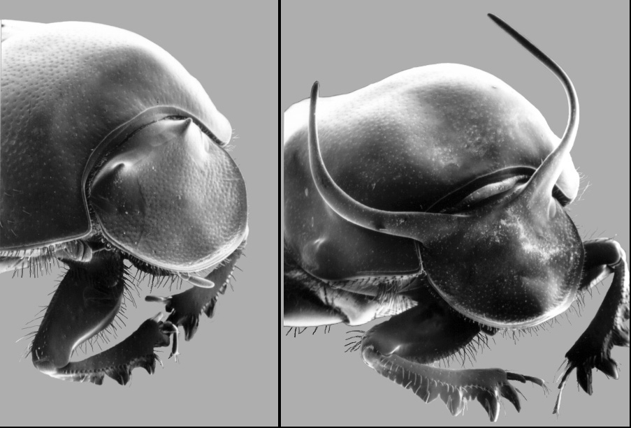
Figure 1: Example of a dimorphic ornament: dung beetles with differing horn lengths (Onthophagus taurus, Coleoptera: Scarabaeidae), reprinted from Emlen:1999vj with permission.

II Model

With the goal of examining the quantitative implications of the handicap principle, we construct a minimal dynamical systems model for the evolution of extravagant and costly ornaments on animals. This proposed model incorporates two components of ornament evolution: an intrinsic cost of ornamentation to an individual (natural selection), and a social benefit of relatively large ornaments within a population (sexual selection). We show that on an evolutionary time scale, identically healthy animals can be forced to split into two morphs, one with large ornaments and one with small.

To express our model, we introduce the idea of a “reproductive potential” $\varphi$. This can be though of as similar to fitness, though our definition differs from the fitness function commonly used in the replicator equation nowak2006 ; karev2010mathematical (we make the relationship between the two explicit in the supplementary information). Over long time scales the effect of evolution is to select for individuals with higher reproductive potential.

Consider an individual reproductive potential $\varphi^{\textrm{(ind)}}$ of a solitary male with ornament size $a$ (e.g., a deer with ornamental antlers). Some ornaments have practical as well as ornamental value (e.g., anti-predation Galeotti:2007fo ; vandenBrink:2012do ), but have a deleterious effect beyond a certain size. We therefore expect that there exists an optimal ornament size (possibly zero), for which individual potential is maximum, and thus take this to be a singly-peaked function of ornament size. For simplicity we assume the quadratic form

$$\varphi^{\textrm{(ind)}}=a(2a_{\textrm{opt}}-a).$$ (1)

Following the handicap principle, we expect the optimal ornament size $a_{\textrm{opt}}=a_{\textrm{opt}}(h)$ to be an increasing function of “intrinsic health” $h$—i.e., healthier individuals can afford larger ornaments. See figure 2 (a) for the general shape of the individual reproductive potential function.

Next, we consider a social reproductive potential $\varphi^{\textrm{(soc)}}$ that captures the effects of competition for partners (i.e., sexual selection). We assume social potential is an increasing function of ornament size because sexual selection often favors larger or more elaborate ornaments Petrie:1994wp . For simplicity, and motivated by the ubiquity of power laws in nature Newman:2005vk ; Reed:2002ua , we choose social potential to be a power of the difference between a male’s ornament size and the average herd ornament size. To ensure monotonicity, we force the social reproductive potential to be antisymmetric about the average ornament size. The social potential is then

$$\varphi^{\textrm{(soc)}}=\operatorname{sgn}{(a-\bar{a})}|a-\bar{a}|^{\gamma},$$ (2)

where the positive parameter $\gamma$ quantifies the rate at which deviations from the mean influence reproductive potential, $\operatorname{sgn}$ is the sign function, and $\bar{a}$ represents the average ornament size in the population. Loosely speaking, the parameter $\gamma$ tunes female choice; we take this “female choice” parameter to be effectively constant because female choice may evolve on a slower time scale than male ornamentation Lande:1981th . Refer to figure 2 (b) for an example of the social reproductive potential function.

Because both natural and sexual selection play a role in the evolution of ornaments Lande:1981th , we take total reproductive potential to be the weighted average

$$\varphi=s\varphi^{\textrm{(soc)}}+(1-s)\varphi^{\textrm{(ind)}},$$ (3)

where $s$ tunes the relative importance of competitive social effects (sexual selection) versus individual effects (natural selection). See figure 2 (c),(d) for examples of total potential functions.

Assuming that evolutionary forces optimize overall reproductive potential at a rate proportional to the marginal benefit of ornamentation, ornament sizes will follow the dynamics

$$\frac{\mathrm{d}a}{\mathrm{d}t}=c\frac{\partial\varphi}{\partial a}$$ (4)

with time-scaling parameter $c>0$. Note that this model does not presume that individual ornaments explicitly change size: the “phenotype flux” $\mathrm{d}a/\mathrm{d}t$ is simply a way of describing how the distribution of ornament sizes in a large animal population changes over long time scales as a result of selection processes.

This results in a piecewise-smooth ordinary differential equation for the ornament size flux,

$$\frac{\mathrm{d}a}{\mathrm{d}t}=c\left[s\gamma\left(1-\frac{1}{N}\right)\left|a-\bar{a}\right|^{\gamma-1}+2(1-s)(a_{\textrm{opt}}-a)\right].$$ (5)

where $N$ is the population size. Plugging (5) into the continuity equation yields a replicator equation for the evolution of the ornament size distribution (see supplementary information).

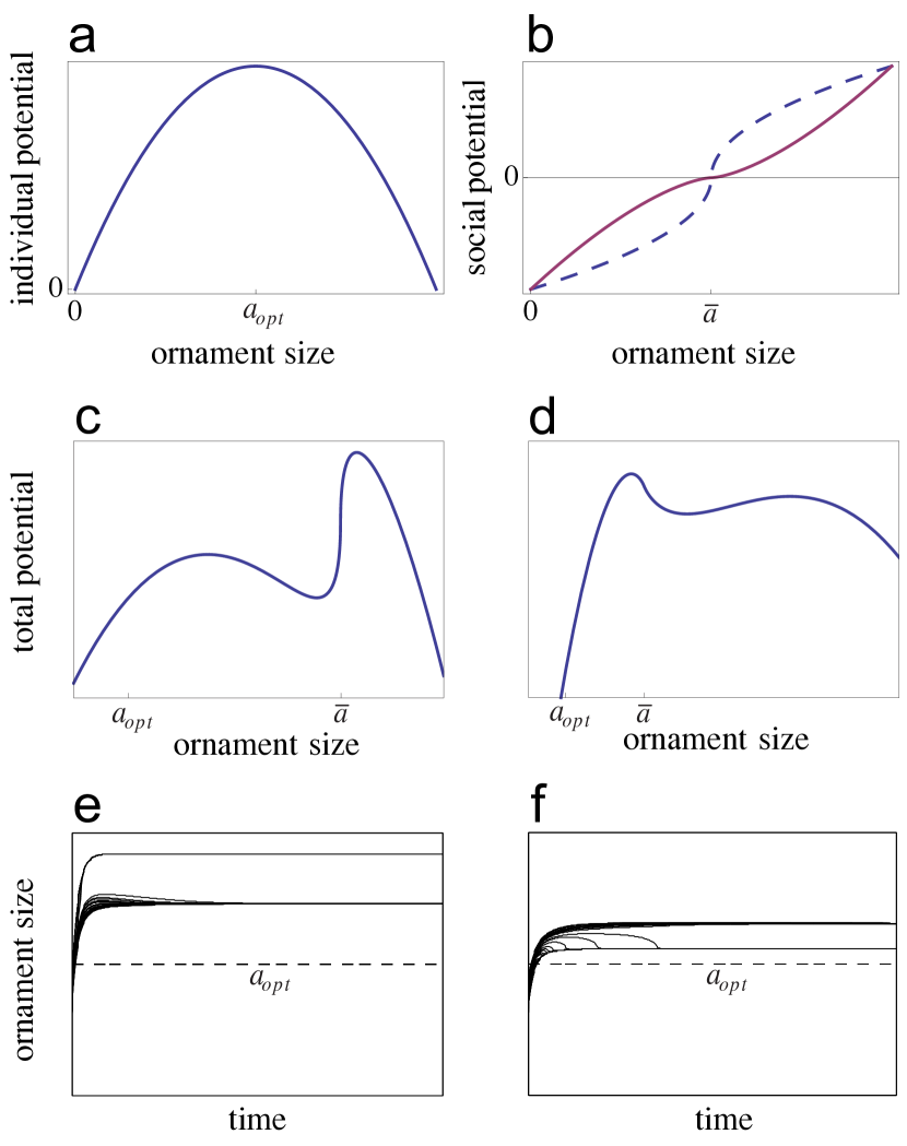
Figure 2: (Color online) Model derivation and behavior. (a) Example individual potential function, singly peaked at $a_{\textrm{opt}}$. We use a quadratic function. (b) Example social potential function, antisymmetric about the population mean $\bar{a}$. We use an anti-symmetrized power law such that the shape depends on the social sensitivity $\gamma$ (blue dashed is $\gamma=0.5$; maroon solid is $\gamma=1.5$). (c) Example total reproductive potential function at equilibrium for $\gamma<1$. There are two local maxima corresponding to two distinct morphs, with the larger ornament morph having the highest potential (here $\gamma=0.5$). (d) Example total potential function at equilibrium for $1<\gamma<2$. There are two local maxima corresponding to two distinct morphs, with the smaller ornament morph having the highest potential (here $\gamma=1.5$). Note that the fitness landscape is distinct for each population representative, and representatives are not assumed to be identical. (e) Evolution of $N=100$ population representatives over time for $\gamma=0.5$ and (f) $\gamma=1.5$. The initial conditions were sampled randomly from a normal distribution with mean 0.75 and standard deviation 0.25. The optimal ornament size $a_{\textrm{opt}}=1.0$, maximum simulation time $t_{max}=50$, time scaling constant $c=1.0$, and $s=1/2$.

III Results

III.1 Numerical exploration

For biologically relevant values of the social sensitivity parameter $\gamma$, our model predicts stratification into distinct phenotypes for a population of identically healthy individuals (i.e., individuals of identical quality). See figure 2 (e),(f) for the time evolution of ornament size for two representative values of $\gamma$.

For $0<\gamma<1$, the ornament sizes stratify into large-ornament and small-ornament groups, with the majority possessing a large-ornament “morph.” For $1<\gamma<2$, the population stratifies into large- and small-ornament morphs, but the majority have small ornaments. The case $\gamma\geq 2$ is not a reasonable option because we have selected a quadratic form for the local approximation of the individual potential function; any power $\gamma$ exceeding 2 implies sexual selection is the dominant evolutionary force even for extremely large ornaments, an unreasonable assumption.

These qualitative results are consistent for all $a_{\textrm{opt}}$ and $0\leq s<1$. While for clarity we have presented predictions of a specific minimal model, the qualitative results hold for a wide range of models. See the Discussion section for the generality of model predictions.

III.2 Analytical results

As numerical integration shows that the uniform and two-morph steady states are of interest, we concentrate our analysis on these equilibria. However, it can also be shown graphically that uniform and two-morph steady states are the only possible solutions for a wide range of potential functions (see supplementary information).

Uniform steady state.

To investigate the uniform equilibrium with an identically healthy population, we set $a=\bar{a}$ producing the single ordinary differential equation,

$$\frac{\mathrm{d}a}{\mathrm{d}t}=2c\,(1-s)(a_{\textrm{opt}}-a).$$ (6)

The steady state (i.e., $\mathrm{d}a/\mathrm{d}t=0$) is clearly $\displaystyle a=a_{\textrm{opt}}$. Linear stability analysis within this identical ornament manifold shows the fixed point $\displaystyle a=a_{\textrm{opt}}$ is stable for all $\gamma$, but numerical simulation suggests that the uniform fixed point is only stable for $\gamma\geq 2$. To resolve this apparent discrepancy, we investigate the uniform fixed point of (5) in the continuum limit, and evaluate stability without restriction to the uniform manifold. We are then able to find $\gamma$-dependence that agrees with simulations (details in supplementary information).

Two-morph steady state.

To investigate the two-morph equilibrium, we assume all males have one of two ornament sizes $a_{1}$ and $a_{2}$. Taking $x$ to be the fraction of males with ornament size $a_{1}$, and $N\to\infty$, the dynamical system becomes

$$\frac{\mathrm{d}a_{1}}{\mathrm{d}t} =\scriptstyle c\Big{[}s\,\gamma\Big{(}(1-x)|a_{1}-a_{2}|\Big{)}^{\gamma-1}+2\,(1-s)(a_{\textrm{opt}}-a_{1})\,\Big{]}$$ (7)

$$\frac{\mathrm{d}a_{2}}{\mathrm{d}t} =\scriptstyle c\Big{[}s\,\gamma\Big{(}x|a_{1}-a_{2}|\Big{)}^{\gamma-1}+2\,(1-s)(a_{\textrm{opt}}-a_{2})\,\Big{]}~{}.$$

There exists one two-morph steady state (i.e., solution to $\mathrm{d}a_{1}/\mathrm{d}t=\mathrm{d}a_{2}/\mathrm{d}t=0$):

$$\scriptstyle a_{1}= \scriptstyle\,a_{\textrm{opt}}+\left(\frac{s\gamma}{2(1-s)}\right)^{\frac{1}{2-\gamma}}\left((1-x)\,\Big{|}\frac{(1-x)^{\gamma}x-x^{\gamma}+x^{1-\gamma}}{(1-x)x}\Big{|}^{\frac{1}{2-\gamma}}\right)^{\gamma-1}$$ (8)

$$\scriptstyle a_{2}= \scriptstyle\,a_{\textrm{opt}}+\left(\frac{s\gamma}{2(1-s)}\right)^{\frac{1}{2-\gamma}}\left(x\,\Big{|}\frac{(1-x)^{\gamma}x-x^{\gamma}+x^{1-\gamma}}{(1-x)x}\Big{|}^{\frac{1}{2-\gamma}}\right)^{\gamma-1}.$$

Figure 3 (a),(b) shows how two-morph equilibria vary with the morph fractionation $x$. Within the shaded region, the fixed point is stable. To be clear, the model predicts that a bimodal population will emerge, with the fraction $x$ of the individuals within the population possessing ornaments of size $a_{1}$. We are not claiming that a proportion $x$ of populations will evolve to ornament size $a_{1}$.

The eigenvalues for the linearized system constrained to this two-morph manifold are $\lambda_{1}=-2(1-s)/s$ and $\lambda_{2}=2(\gamma-2)(1-s)/s$. Clearly, the two-morph equilibrium is stable (within the two-morph manifold) for $0<\gamma<2$ and unstable for $\gamma>2$, when $\lambda_{2}>0$. Curiously, the stability of the two-morph equilibrium does not depend on $x$, the morph fractionation. This presents an apparent problem because numerical simulation suggests that only certain ranges of $x$ are stable: see figure 3 (c). Similarly to the uniform fixed point analysis, we investigate the fixed points of the model in the continuum limit, and evaluate stability without restriction to any manifold. We are then able to find $x$-dependence that agrees well with simulations: see figure 3 (d) (details in supplementary information).

Figure 3: Stability regions for two-morph steady states ($N=100$, $s=1/2$). The ornament size for morph 1 is blue (dashed line), and the ornament size for morph 2 is maroon (solid line). The shaded regions are stable. (a) Two morph steady state for various morph fractionation $x$ and $\gamma=0.5$ (b) Two morph steady state for various morph fractionation $x$ and $\gamma=1.5$. (c) Analytical stability region (grey shading) for finite $N$ model within two-morph manifold with numerical stability region (dots) superimposed. (d) Analytical stability region (grey shading) from continuum model with numerical stability region (dots) superimposed.

IV Model Validation

We now revisit our simplifying assumption that all males are equally healthy. More realistically, we allow the intrinsic health $h$ to be taken from some distribution (perhaps set by genetic, developmental, or environmental factors). Suppose this distribution is such that the individual optimal ornament size $a_{\textrm{opt}}(h)$ is normally distributed. Then the stable two-morph steady state changes from a weighted sum of perfectly narrow Dirac delta functions to a distribution roughly resembling the sum of two Gaussians—usually a bimodal distribution. Marginal histograms in figure 4 (a),(b) show examples of steady states with varied intrinsic health.

These examples resemble data from many species that grow ornaments. Figure 4 (c),(d) show two examples of real-world ornament distributions that exhibit bimodality. Note that we do not expect the exact shape of the real-world distributions to match our simulations because the measured quantities will not necessarily be linear in cost. However, bimodality will be preserved regardless of the measured quantity.

In a literature search Searcy:1990ta ; Norris:1990uy ; Bortolotti:2006co ; BADYAEV:2000jy ; Niecke:2003gi ; Andersson:2002gn ; Petrie:1994wp ; Loyau:2005dc ; MaysJr:2004vg ; Pelabon:1998vo ; West:2002cp ; Moczek:2002vm ; Barber:2001vm ; Hyatt:1978tw ; Tomkins:2005jf ; Skarstein:1996uc , we found a number of published data sets showing size distributions of suspected ornaments; 23 were of sufficient quality for testing agreement with this model. In 13 of those data sets we found some evidence for rejecting the hypothesis of unimodality: the data were more consistent with a mixture of two or more Gaussian distributions than with a single Gaussian. In seven data sets, we found stronger evidence: non-parametric tests rejected the hypothesis of unimodality. Note that other data sets were not inconsistent with bimodality, but small sample sizes often limited the power of statistical testing. See supplementary information for histograms and statistical tests of additional data sets.

V Discussion

V.1 Implications for honest signaling

Assuming this model adequately represents the handicap principle, we may ask if ornament size really does honestly advertise quality. In other words, if a female can choose among all the males, is she able to detect the healthiest (or weakest) males simply by looking at ornament size? Again taking the optimal ornament size $a_{\textrm{opt}}$ to be normally distributed, we examine the Kendall rank correlation between intrinsic health (as indicated by our proxy $a_{\textrm{opt}}$) and equilibrium ornament size.

We find that the advertising is mostly honest, at least for large enough variance in health. Both observational and experimental work supports this finding Johnstone:1995wt . Figure 4 (a),(b) show examples of ornament size versus intrinsic health based on our model.

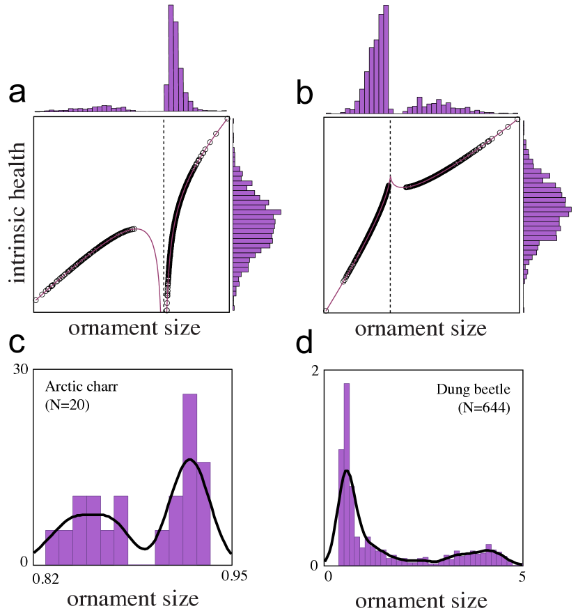
Figure 4: Ornament size distributions in model and real-world data. Due to smaller sample sizes in real-world data, we superimpose a kernel density estimate (KDE) over the histograms as a visual aid (solid black line). (a) Simulation of model with $N=1000$ individuals, $\gamma=0.5$, $s=1/2$ (Kendall’s rank correlation $\tau=0.9149$). (b) Simulation of model with $N=1000$ individuals, $\gamma=1.5$, $s=1/2$ (Kendall’s rank correlation $\tau=0.9998$). In both (a) and (b), black dashed line ($a=\bar{a}$) shows division between morphs, solid maroon curve shows analytical solution. Marginal histograms illustrate that normal distribution of $a_{\textrm{opt}}$ (proxy for intrinsic health) leads to bimodal distribution of $a$. (c) Normalized histogram for arctic charr brightness Skarstein:1996uc ($N$=20, KDE bandwidth=0.01). (d) Normalized histogram for dung beetle horn length Moczek:2002vm ($N$=644, KDE bandwidth=0.2).

V.2 Generality

It is natural to wonder about the generality of the results we have presented here. For a reasonable set of potential functions (described below), the only possible stable equilibria are multimodal distributions of ornament size. The following are the requirements for our reasonable potential functions:

1. Individual effects dominate potential for large ornament sizes. Specifically,

   $$(1-s)\left|\frac{\partial}{\partial a}\varphi^{\textrm{(ind)}}\right|>s\left|\frac{\partial}{\partial a}\varphi^{\textrm{(soc)}}\right|\text{ as }a\to\infty.$$

   This prevents ornament size from growing without bound, as can occur in model (5) for $\gamma\geq 2$ (see figure 2 (e)).

2. Social effects dominate potential for at least some range of ornament sizes greater than the population mean. In other words,

   $$(1-s)\left|\frac{\partial}{\partial a}\varphi^{\textrm{(ind)}}\right|<s\left|\frac{\partial}{\partial a}\varphi^{\textrm{(soc)}}\right|$$

   for at least some range of $a>\bar{a}$. Failure to meet this criterion could be considered “false” ornamentation, as in model (5) for $\gamma=1$.

Assuming the potential functions are continuous, these criteria guarantee that two or more morphs will emerge (see supplementary information for details).

VI Conclusions

The independent evolution of costly ornamentation across species has puzzled scientists for over a century. Several general evolutionary principles have been proposed to explain this phenomenon. Among the prominent hypotheses is the handicap principle, which posits that only the healthiest individuals can afford to grow and carry large ornaments, thereby serving as honest advertising to potential mates. We base a minimal model on this idea and find that, surprisingly, it predicts two-morph stratification of ornament size, which appears to be common in nature.

Importantly, the two morphs both have ornament sizes larger than the optimum for lone individuals. This means that the population survival potential, as indicated by the population average of individual potential $\displaystyle\overline{\varphi}^{(ind)}$, is reduced. Due to the presence of ornaments, we conclude that the evolutionary benefits of honest advertising must outweigh the net costs of ornamentation when the displays exist in nature.

VII Author Contributions

S.M.C. and D.M.A. developed and analyzed the model, S.M.C. implemented the numerical simulations and created the database, R.I.B. and S.M.C. performed statistical tests on data.

VIII Data Accessibility

Data and code available from the Dryad Digital Repository dryadDataSoftware : http://dx.doi.org/10.5061/dryad.vb1pp.

IX Competing Interests

The authors have no competing interests.

X Acknowledgments

We thank Daniel Thomas, Trevor Price and Stephen Pruett-Jones for valuable discussions and Doug Emlen, Craig Packer, Markus Eichhorn, and Armin Moczek for sharing biological data.

XI Funding

This research was supported in part by James S. McDonnell Foundation Grant No. 220020230 and National Science Foundation Graduate Research Fellowship No. DGE-1324585.

in 1,…,14 See pages \x, of SCRBDA-ornament-preprint-arxiv-SI-final.pdf

References

- (1) C. Darwin, The descent of man and selection in relation to sex. John Murray, 1871.
- (2) M. Andersson and L. W. Simmons, “Sexual selection and mate choice,” Trends in Ecology & Evolution, vol. 21, no. 6, pp. 296–302, 2006.
- (3) T. Clutton-Brock, “Sexual Selection in Males and Females,” Science, vol. 318, no. 5858, pp. 1882–1885, 2007.
- (4) A. G. Jones and N. L. Ratterman, “Mate choice and sexual selection: what have we learned since Darwin?,” Proceedings of the National Academy of Sciences, vol. 106, no. Supplement 1, pp. 10001–10008, 2009.
- (5) A. Zahavi, “Mate selection—a selection for a handicap,” Journal of Theoretical Biology, vol. 53, no. 1, pp. 205–214, 1975.
- (6) B. J. Allen and J. S. Levinton, “Costs of bearing a sexually selected ornamental weapon in a fiddler crab,” Functional Ecology, vol. 21, no. 1, 2007.
- (7) M. R. Evans and A. L. Thomas, “The aerodynamic and mechanical effects of elongated tails in the scarlet-tufted malachite sunbird: measuring the cost of a handicap,” Animal Behaviour, vol. 43, no. 2, pp. 337–347, 1992.
- (8) J. Goyens, S. Van Wassenbergh, J. Dirckx, and P. Aerts, “Cost of flight and the evolution of stag beetle weaponry,” Journal of The Royal Society Interface, vol. 12, no. 106, pp. 20150222–20150222, 2015.
- (9) R. A. Johnstone, “Sexual selection, honest advertisement and the handicap principle: reviewing the evidence,” Biological Reviews, vol. 70, no. 1, pp. 1–65, 1995.
- (10) J. D. Blount, N. B. Metcalfe, T. R. Birkhead, and P. F. Surai, “Carotenoid modulation of immune function and sexual attractiveness in zebra finches,” Science, vol. 300, no. 5616, pp. 125–127, 2003.
- (11) P. M. West, “Sexual Selection, Temperature, and the Lion’s Mane,” Science, vol. 297, no. 5585, pp. 1339–1343, 2002.
- (12) M. Petrie and T. Halliday, “Experimental and natural changes in the peacock’s (Pavo cristatus) train can affect mating success,” Behavioral Ecology and Sociobiology, vol. 35, no. 3, pp. 213–217, 1994.
- (13) M. Andersson, “Female choice selects for extreme tail length in a widowbird,” Nature, vol. 299, no. 5886, pp. 818–820, 1982.
- (14) B. Kuijper, I. Pen, and F. J. Weissing, “A guide to sexual selection theory,” Annual Review of Ecology, Evolution, and Systematics, vol. 43, pp. 287–311, 2012.
- (15) S. Collins, “Is there only one type of male handicap?,” Proceedings of the Royal Society of London B: Biological Sciences, vol. 252, no. 1335, pp. 193–197, 1993.
- (16) H. Kokko, M. D. Jennions, and R. Brooks, “Unifying and testing models of sexual selection,” Annual Review of Ecology, Evolution, and Systematics, pp. 43–66, 2006.
- (17) G. E. Hill and K. Yasukawa, “The evolution of ornaments and armaments,” Animal Behavior: How and Why Animals Do the Things They Do, vol. 2, pp. 145–172, 2014.
- (18) H. Gintis, E. A. Smith, and S. Bowles, “Costly signaling and cooperation,” Journal of theoretical biology, vol. 213, no. 1, pp. 103–119, 2001.
- (19) A. Grafen, “Biological signals as handicaps,” Journal of theoretical biology, vol. 144, no. 4, pp. 517–546, 1990.
- (20) Y. Iwasa, A. Pomiankowski, and S. Nee, “The evolution of costly mate preferences ii. the’handicap’principle,” Evolution, pp. 1431–1442, 1991.
- (21) R. Lande, “Models of speciation by sexual selection on polygenic traits,” Proceedings of the National Academy of Sciences, vol. 78, no. 6, part 2, pp. 3721–3725, 1981.
- (22) M. A. Nowak, Evolutionary Dynamics. Harvard University Press, 2006.
- (23) U. Dieckmann and R. Law, “The dynamical theory of coevolution: a derivation from stochastic ecological processes,” Journal of mathematical biology, vol. 34, no. 5-6, pp. 579–612, 1996.
- (24) D. J. Emlen and H. F. Nijhout, “Hormonal control of male horn length dimorphism in the dung beetle Onthophagus taurus(Coleoptera: Scarabaeidae),” Journal of Insect Physiology, vol. 45, no. 1, pp. 45–53, 1999.
- (25) A. Aisenberg and F. G. Costa, “Reproductive isolation and sex-role reversal in two sympatric sand-dwelling wolf spiders of the genus Allocosa,” Canadian Journal of Zoology, vol. 86, no. 7, pp. 648–658, 2008.
- (26) J. L. Tomkins, J. S. Kotiaho, and N. R. LeBas, “Matters of Scale: Positive Allometry and the Evolution of Male Dimorphisms,” The American Naturalist, vol. 165, no. 3, pp. 389–402, 2005.
- (27) K. A. Glover, O. T. Skilbrei, and Ø. Skaala, “Stock-specific growth and length frequency bimodality in brown trout,” Transactions of the American Fisheries Society, vol. 132, no. 2, pp. 307–315, 2003.
- (28) K. A. Glover, C. Skår, K. E. Christie, J. Glette, H. Rudra, and Ø. Skaala, “Size-dependent susceptibility to infectious salmon anemia virus (ISAV) in Atlantic salmon (Salmo salar L.) of farm, hybrid and wild parentage,” Aquaculture, vol. 254, no. 1-4, pp. 82–91, 2006.
- (29) M. J. West-Eberhard, “Sexual selection and social behavior,” Man and Beast Revisited, pp. 159–172, 1991.
- (30) M. R. Gross, “Alternative reproductive strategies and tactics: diversity within sexes,” Trends in Ecology & Evolution, vol. 11, no. 2, pp. 92–98, 1996.
- (31) G. P. Karev, “On mathematical theory of selection: continuous time population dynamics,” Journal of mathematical biology, vol. 60, no. 1, pp. 107–129, 2010.
- (32) P. Galeotti and D. Rubolini, “Head ornaments in owls: what are their functions?,” Journal of Avian Biology, vol. 38, no. 6, pp. 731–736, 2007.
- (33) V. van den Brink, V. Dolivo, X. Falourd, A. N. Dreiss, and A. Roulin, “Melanic color-dependent antipredator behavior strategies in barn owl nestlings,” Behavioral Ecology, vol. 23, no. 3, pp. 473–480, 2012.
- (34) M. E. Newman, “Power laws, pareto distributions and zipf’s law,” Contemporary Physics, vol. 46, no. 5, pp. 323–351, 2005.
- (35) W. J. Reed and B. D. Hughes, “From gene families and genera to incomes and internet file sizes: Why power laws are so common in nature,” Physical Review E, vol. 66, no. 6, p. 067103, 2002.
- (36) T. Getty, “Sexually selected signals are not similar to sports handicaps,” Trends in Ecology & Evolution, vol. 21, no. 2, pp. 83–88, 2006.
- (37) W. A. Searcy, “Species recognition of song by female red-winged blackbirds,” Animal Behaviour, vol. 40, no. 6, pp. 1119–1127, 1990.
- (38) K. J. Norris, “Female choice and the quality of parental care in the great tit Parus major,” Behavioral Ecology and Sociobiology, vol. 27, no. 4, pp. 275–281, 1990.
- (39) G. R. Bortolotti, J. Blas, J. J. Negro, and J. L. Tella, “A complex plumage pattern as an honest social signal,” Animal Behaviour, vol. 72, no. 2, pp. 423–430, 2006.
- (40) A. Badyaev, “Evolution of sexual dichromatism: contribution of carotenoid- versus melanin-based coloration,” Biological journal of the Linnean Society, vol. 69, no. 2, pp. 153–172, 2000.
- (41) M. Niecke, S. Rothlaender, and A. Roulin, “Why do melanin ornaments signal individual quality? Insights from metal element analysis of barn owl feathers,” Oecologia, vol. 137, no. 1, pp. 153–158, 2003.
- (42) S. Andersson, S. R. Pryke, J. Örnborg, M. J. Lawes, and M. Andersson, “Multiple Receivers, Multiple Ornaments, and a Trade-off between Agonistic and Epigamic Signaling in a Widowbird,” The American Naturalist, vol. 160, no. 5, pp. 683–691, 2002.
- (43) A. Loyau, M. Saint Jalme, C. Cagniant, and G. Sorci, “Multiple sexual advertisements honestly reflect health status in peacocks (Pavo cristatus),” Behavioral Ecology and Sociobiology, vol. 58, no. 6, pp. 552–557, 2005.
- (44) H. L. Mays, Jr, K. J. McGraw, G. Ritchison, S. Cooper, V. Rush, and R. S. Parker, “Sexual dichromatism in the yellow-breasted chat Icteria virens: spectrophotometric analysis and biochemical basis,” Journal of Avian Biology, vol. 35, no. 2, pp. 125–134, 2004.
- (45) C. Pélabon and L. van Breukelen, “Asymmetry in antler size in roe deer (Capreolus capreolus): an index of individual and population conditions,” Oecologia, vol. 116, no. 1-2, pp. 1–8, 1998.
- (46) A. P. Moczek and H. F. Nijhout, “Developmental mechanisms of threshold evolution in a polyphenic beetle,” Evolution & Development, vol. 4, no. 4, pp. 252–264, 2002.
- (47) I. Barber, D. Nairn, and F. A. Huntingford, “Nests as ornaments: revealing construction by male sticklebacks,” Behavioral Ecology, vol. 12, no. 4, pp. 390–396, 2001.
- (48) G. W. Hyatt and M. Salmon, “Combat in the fiddler crabs Uca pugilator and U. pugnax: a quantitative analysis,” Behaviour, vol. 65, no. 1, pp. 182–211, 1978.
- (49) F. Skarstein and I. Folstad, “Sexual dichromatism and the immunocompetence handicap: an observational approach using arctic charr,” Oikos, vol. 76, pp. 359–367, 1996.
- (50) S. M. Clifton, R. I. Braun, and D. M. Abrams, “Data from: Handicap principle implies emergence of dimorphic ornaments.”