Linear Arrangement of Halin Graphs

Abstract

We study the Optimal Linear Arrangement (OLA) problem of Halin graphs, one of the simplest classes of non-outerplanar graphs. We present several properties of OLA of general Halin graphs. We prove a lower bound on the cost of OLA of any Halin graph, and define classes of Halin graphs for which the cost of OLA matches this lower bound. We show for these classes of Halin graphs, OLA can be computed in $O(n\log{n})$, where $n$ is the number of vertices.

1 Introduction

Given graph $G=(V,E)$, a linear arrangement or simply a layout of vertices is defined as a bijective function $\varphi:V\rightarrow\{1,\dots,|V|\}$. In the Optimal Linear Arrangement (OLA) problem, a special case of more general vertex layout problems, the goal is to find the layout $\varphi$ minimizing $\sum_{\{v,u\}\in E}|\varphi(v)-\varphi(u)|$. The OLA problem is known to be NP-hard for general graphs [5], for bipartite graphs [4], and for more specific classes of graphs such as interval graphs and permutation graphs [2].

Defining interesting classes of graphs for which the OLA problem is polynomially solvable has been a notoriously hard task. The results have been few and spread over several decades [5, 4, 2, 1, 10]. Three decades ago, it was suggested that a good candidate for polynomial-solvable OLA are interval graphs, a class of graph for which no NP-hardness results were known at that time (page 13 of [8]). Efforts in that direction were in vain, as some two decades later, the OLA problem of interval graphs was shown to be NP-hard [2]. Another candidate for polynomial-solvable OLA are the so-called recursively constructed graphs [7], given that most NP-hard problems on general graphs are easily solvable for this class.

Halin graphs are planar graphs which the degree of every vertex is at least 3 and can be constructed using an underlying tree $T$ and a cycle $C$ which connects leaf nodes of the tree $T$. Figure 1 presents a Halin graph. Throughout this report, the edges of cycle $C$ are presented in bold and the edges of the tree $T$ are depicted in dashed lines. Halin graphs can be considered as one of the simplest class of graphs that are not outerplanar .

To the best of our knowledge, the OLA problem of Halin graphs is only studied for the simple case where the underlying tree is a caterpillar  [3]. After introducing our notations and preliminary definitions in Section 2, we present several properties of OLA of Halin graphs in Section 3, including a lower bound on the cost of OLA for Halin graphs. In Section 4, we define and study a class of Halin graphs for which the cost of their OLA meets this lower bound. We also present an algorithm which, given a Halin graph in this class, returns an OLA in $O(n\log{n})$ where $n$ is the number of vertices.

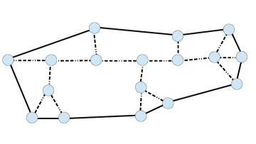
Figure 1: $H_{1}$, an example of a Halin graph. The cycle which connect the leaf nodes is shown in bold and the underlying tree is presented in dashed lines.

2 Preliminaries

We only consider simple, undirected graphs. For a finite graph $G=(V,E)$ where $V$ and $E$ are respectively the sets of vertices and edges, we show $|V|$ by $n$ and $|E|$ as $m$. For a given vertex $v\in V$, $d_{G}(v)$ presents the degree of $v$ in $G$. For a subgraph $G^{\prime}\subseteq G$, $V(G^{\prime})$ and $E(G^{\prime})$ respectively present the set of vertices and edges of $G^{\prime}$.

We denote by $\Phi(G)$ the set of all possible layouts for the graph $G$. A layout $\varphi$ can be considered as an ordering $(w_{1},w_{2},\ldots,w_{n})$ of vertices of $V$. Accordingly for $v=w_{i}\in V$, $\varphi(v)=i$. Without loss of generality we assume the left most and right most vertices are recursively labeled as $1$ and $n$ and we call them the extreme vertices based on $\varphi$.

Notation 2.1.

Let $V_{1},\ldots,V_{k}$ be a partitioning of $V$. We say a layout $\varphi$ is of type $(V_{1},V_{2},\ldots,V_{k})$ if:

$$\forall 1\leq i<j\leq k,\forall v\in V_{i},\forall u\in V_{j}\Rightarrow\varphi(v)<\varphi(u)$$

Notation 2.2.

Given layout $\varphi$ for $G=(V,E)$ and an edge $e=\{u,v\}\in E$ we define the expand of $e$ as:

$$\lambda(e,\varphi)=|\varphi(u)-\varphi(v)|$$

Several cost functions have been defined on a given graph $G$ and layout $\varphi$. For a comprehensive list refer to [9]. In this report we focus on $OptimalLinearArrangement$ problem (OLA) defined as follows.

Definition 2.3 (Optimal Linear Arrangement).

Given an undirected graph $G=(V,E)$ and a layout $\varphi$ the linear arrangement cost (LA) of $\varphi$ is:

$$LA(\varphi,G)=\sum_{\{v,u\}\in E(G)}\lambda(\{u,v\},\varphi)$$

A layout $\varphi^{*}$ is optimal if:

$$LA(\varphi^{*},G)=\min_{\varphi\in\Phi(G)}{LA(\varphi,G)}$$

$\square$

Lemma 2.4 present a lower bound on the cost of optimal linear arrangement which will be useful in presenting some properties and proofs in the rest of the paper.

Lemma 2.4.

Given graph $G=(V,E)$ and two induced subgraph $G_{1}=(V,E_{1})$ and $G_{2}=(V,E_{2})$ s.t. $E_{1}\cap E_{2}=\emptyset$ and $E_{1}\uplus E_{2}=E$, assume $\varphi^{*}$, $\varphi^{*}_{1}$ and $\varphi^{*}_{2}$ are respectively the optimal linear arrangement for $G$, $G_{1}$ and $G_{2}$.Then $LA(\varphi,G)\geq LA(\varphi^{*}_{1},G_{1})+LA(\varphi^{*}_{2},G_{2})$.

A Halin graph $H=(V,E)$ is constructed based on an underlying tree $T=(V,E^{\prime})$ embedded in plane in a planar manner where all the leaf nodes are connected using a cycle $C=(V^{\prime},E^{\prime\prime})$. A Halin graph $H$ is shown as $H=T\uplus C$. As depicted in Figure 2 it’s easy to see that for a given tree $T$, there may exist finitely many non-isomorphic Halin graphs.

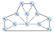
(a) Halin graph $H_{2}$

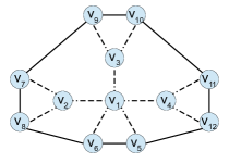
(b) Halin graph $H_{3}$

Figure 2: Two non-isomorphic Halin graphs constructed from the same tree using different embedding.

Based on the structure of Halin graphs, one may suspect that they inherit many of properties of their underlying tree. Accordingly in the following subsection we present some properties and well-known facts regarding the OLA of trees.

2.1 Linear Arrangement of Trees

As one of non-trivial results, the OLA of trees was first shown to be polynomially solvable in [6] and more efficient algorithms were later presented in [11, 1]. In this section we present some well-known properties of OLA of trees which simplify the understanding of linear arrangement of Halin graphs in the rest of the report. For more details, one can refer to  [1].

Property 2.5.

Given an OLA $\varphi^{*}$ for tree $T=(V,E)$, vertices that are assigned label $1$ and $n$ are leaf nodes (the two extreme vertices are leafs in $T$). $\square$

Definition 2.6 (Spinal path).

Given layout $\varphi$ for a tree $T=(V,E)$, and vertices $v,u\in V$ where $\varphi(v)=1$ and $\varphi(u)=n$, we define the path $P=(w_{1}=v,w_{2},\dots,w_{l}=u)$ connecting $v$ and $u$, the spine of tree $T$ corresponding to $\varphi$. $\square$

Property 2.7.

Having OLA $\varphi^{*}$ for tree $T=(V,E)$ and spinal path $P=(w_{1}=v,w_{2},\dots,w_{l}=u)$, it is the case that $\forall 1\leq i<l:\varphi^{*}(w_{i})<\varphi^{*}(w_{i+1})$. In other word, the function $\varphi^{*}$ is monotonic along the path $P$. $\square$

Definition 2.8 (Spinal rooted subtree and anchored branches).

Given layout $\varphi$ for a tree $T=(V,E)$ and spinal path $P=(w_{1}=v,w_{2},\dots,w_{l}=u)$, Removing all edges of $P$, leaves us with a set of subtrees $T_{1},T_{2},\ldots,T_{l}$ respectively rooted at $w_{1},w_{2},\dots,w_{l}$. Removing spinal vertex $w_{i}$ from $T_{i}$ where $d_{T}(w_{i})=k>2$, results in a set of branches $B_{i,1},B_{i,2},\ldots,B_{i,k-2}$. Each branch $B_{i,j}$ is anchored at a vertex $v_{j}$ which is connected to $w_{i}$. $\square$

Property 2.9.

Consider a tree $T=(V,E)$ and its OLA $\varphi^{*}$ and the corresponding spinal path $P=(w_{1}=v,w_{2},\dots,w_{l}=u)$. Removing all the edges of $P$ results in a set of $l$ subtrees $T_{1},\ldots,T_{l}$, respectively rooted at $w_{1},\ldots,w_{l}$. Then based on $\varphi^{*}$, for a fixed $i$, the vertices of of $T_{i}$ are labeled by contentious integers. Formally speaking:

$$\forall 1<i<l,\forall u\in T_{i-1},v\in T_{i},w\in T_{i+1}\Rightarrow\varphi^{*}(u)<\varphi^{*}(u)<\varphi^{*}(w)$$

Moreover $\varphi^{*}$ restricted to $V(T_{i})$ (denoted by $\varphi^{*}_{i}$) is optimal for $T_{i}$. $\square$

3 Some Properties of OLA of Halin Graphs

Halin graphs are the example of edge-minimal 3-connected graphs.Hence, in a Halin graph $H=T\uplus C$, for any two vertices $v$ and $u$, there are exactly three edge-disjoint paths connecting $v$ and $u$ where one comprises only edges of $E(T)$.

Definition 3.1 (Spinal path in Halin graphs).

Given layout the $\varphi$ for a Halin graph $H$ and two vertices $v,u\in E(H)$ where $\varphi(v)=1$ and $\varphi(u)=n$, the spinal path based on $\varphi$, is defined as the path $P=(w_{1}=v,w_{2},\dots,w_{l}=u)$ where for every $1\leq i<l$, $\{w_{i},w_{i+1}\}$ is an edge in $T$. $\square$

Definition 3.2 (Spinal rooted subtree and anchored branches in Halin graphs).

Given layout $\varphi$ for a a Halin graph $H=T\uplus C$ and spinal path $P=(w_{1}=v,w_{2},\dots,w_{l}=u)$, removing all edges of $P$ and $E(C)$ results in a set of subtrees $T_{1},T_{2},\ldots,T_{l}$, respectively rooted at $w_{1},w_{2},\dots,w_{l}$. Removing spinal vertex $w_{i}$ from $T_{i}$ where $d_{T}(w_{i})=k>2$, give us a set of branches $B_{i,1},B_{i,2},\ldots,B_{i,k-2}$. Also each branch $B_{i,j}$ is anchored at a vertex $v_{j}$, connected to $w_{i}$. $\square$

Lemma 3.3.

Consider the Halin graph $H=T\uplus C$ and the spinal path $P=(w_{1},w_{2},\dots,w_{l})$ based on a given OLA $\varphi^{*}$. Removing all the edges of $P$ and $C$ results in a set of $l$ subtrees $T_{1},\ldots,T_{l}$ respectively rooted at $w_{1},\ldots,w_{l}$. For a fixed $i$, the vertices of of $T_{i}$ are labeled by contentious integers by OLA $\varphi^{*}$. Formally speaking:

$$\forall 1<i<l,\forall u\in T_{i-1},v\in T_{i},w\in T_{i+1}\Rightarrow\varphi^{*}(u)<\varphi^{*}(u)<\varphi^{*}(w)$$

See proof A.6 in Appendix A.

Corollary 3.4.

Having OLA $\varphi^{*}$ for Halin graph $H$ and spinal path $P=(w_{1},w_{2},\dots,w_{l})$, it is the case that $\forall 1\leq i<l:\varphi^{*}(w_{i})<\varphi^{*}(w_{i+1})$. In other word, the function $\varphi^{*}$ is monotonic along the path $P$.

Lemma 3.5.

Consider an OLA $\varphi^{*}$ for a Halin graph $H=T\uplus C$ and the set of subtrees $T_{1},\ldots,T_{l}$ resulted after removing the edges of $C$ and the spinal path $P=(w_{1},w_{2},\dots,w_{l})$. Let $\{B_{i,1},\dots,B_{i,k-2}\}$ be the set of branches of $T_{i}$ connected to a spinal vertex $w_{i}$ with degree $k>2$. For two branches $B_{i,j}$ and $B_{i,j^{\prime}}$:

• If $\varphi^{*}$ is of type $(\ldots,w_{i},\ldots,V(B_{i,j})\cup V(B_{i,j^{\prime}}),\ldots)$ then it is of type $(\ldots,w_{i},\ldots,V(B_{i,j}),V(B_{i,j^{\prime}}),\ldots)$ or $(\ldots,w_{i},\ldots,V(B_{i,j^{\prime}}),V(B_{i,j}),\ldots)$

• If $\varphi^{*}$ is of type $(\ldots,V(B_{i,j})\cup V(B_{i,j^{\prime}}),\ldots,w_{i},\ldots)$ then it is of type $(\ldots,V(B_{i,j}),V(B_{i,j^{\prime}}),\ldots,w_{i},\ldots)$ or $(\ldots,V(B_{i,j^{\prime}}),V(B_{i,j}),\ldots,w_{i},\ldots)$

In other word the two branches $B_{i,j}$ and $B_{i,j^{\prime}}$ which are on the same side of $w_{i}$ (either their vertices are all labeled after $w_{i}$ or all before it), do not overlap.

For proof refer to Appendix A, proof A.11.

Theorem 3.6.

Given an OLA $\varphi^{*}$ for a Halin graph $H=T\uplus C$ and the vertices $v$ and $u$ where $\varphi^{*}(v)=1$ and $\varphi^{*}(u)=n$, it is always the case that:

• $v$ and $u$ are both leaves in $T$ or

• if $v$ (or $u$) is not a leaf vertex in $T$, then degree of $v$ is three and it is connected to exactly two leaves in $T$. Accordingly replacing the label of $v$ (or $u$) with one of it’s leaf nodes, we get another OLA $\varphi^{\circledast}$ where the extreme nodes are leaves in $T$.

This lemma is proven in proof A.15 in Appendix A.

Corollary 3.7.

Consider an OLA $\varphi^{*}$ for a Halin graph $H=(V,E)$ constructed from tree $T=(V,E^{\prime})$ and cycle $C$, then:

$$LA(\varphi^{*},H)\geq 2\times(n-1)+LA(\varphi_{T}^{*},T)$$

where $\varphi_{T}^{*}$ is the OLA for $T$.

4 Halin Graphs With Polynomially Solvable LA Algorithm

As mentioned before, the OLA problem is polynomially solvable for trees. The OLA of a Halin graph $H=T\uplus C$, depends both on the underlying tree and the planar embedding of $T$. Motivated by the work in [11], in this section we study some classes of Halin graphs where OLA problem can be solved in polynomial time. More specifically we show that for these classes of Halin graphs, the equality in corollary 3.7 holds.

Definition 4.1 (Recursively Balanced Trees).

Consider the tree $T$ and the vertex $v_{r}$, designated as the root of the tree, and the set of vertices $v_{r,0},\ldots,v_{r,k}$ connected to the $v_{r}$ as it’s direct children. Removing the set of edges $\{v_{r},v_{r,0}\},\ldots,\{v_{r},v_{r,k}\}$ results in the set of subtrees $T_{r,0},\ldots,T_{r,k}$, respectively rooted at $v_{r,0},\ldots,v_{r,k}$. $T$ is recursively balanced if:

• $\mathcal{T}_{r,0}=\mathcal{T}_{r,1}=\ldots=\mathcal{T}_{r,k}$ and

• $T_{r,i}$, rooted at $v_{r,i}$, is recursively balanced for $i=0,1,\ldots,k$

$\square$

The root vertex $v_{r}$ of a Recursively Balanced Tree (RBT), is the only vertex satisfying the properties of the central vertex in the following theorem.

Theorem 4.2.

Given a tree $T=(V,E)$, there exists a vertex $v_{r}$ where the set of subtrees $T_{0},\ldots,T_{k}$ resulted by removing $v_{r}$ from $T$, satisfies:

$$\mathcal{T}_{i}\leq\lfloor\dfrac{n}{2}\rfloor \quad\text{for}\quad i=0,\ldots,k$$

For proof see [11].

Considered a tree $T$ rooted at $v_{r}$ and the corresponding subtrees $T_{0},\ldots,T_{k}$ after removing $v_{r}$, where $\mathcal{T}_{0}\geq\mathcal{T}_{2}\geq\ldots\geq\mathcal{T}_{k}$. Assume that an OLA $\varphi^{*}$ for $T$ is of type $(\ldots,T_{i},\ldots,v_{r},\ldots)$ or $(\ldots,v_{r},\ldots,T_{i},\ldots)$ for some subtree $T_{i}$. $T_{i}$ is called (respectively right or left) anchored subtree, rooted at $v_{i}$ connecting $T_{i}$ to $v_{r}$. A tree $T$ which is not anchored is called a free tree. In theorem 4.3, which is the motivating theorem and the heart of the OLA algorithm for trees in [11], we show the root of a tree by $v_{r}$. Vertex $v_{r}$ is the central vertex in the case of free trees, or the anchor vertex if the tree is an anchored subtree. Also the parameter $\alpha$ is $0$ for free trees and $1$ otherwise.

Theorem 4.3.

Given a free or (right) anchored tree $T=(V,E)$ , let $\rho$ be the largest integer that satisfies the following:

$$\mathcal{T}_{i}>\lfloor\dfrac{\mathcal{T}_{1}+2}{2}\rfloor+\lfloor\dfrac{\mathcal{T}_{*}+2}{2}\rfloor\quad\text{for}\quad i=1,\ldots,2\rho-\alpha$$

where:

$$\mathcal{T}_{*}=n-\sum\limits_{0}^{2\rho-\alpha}\mathcal{T}_{i}$$

• If $\rho=0$, the OLA of $T$ is of type $(T_{0},v_{r},\ldots)$

• If $\rho>0$, then $T$ has an OLA of type either $(T_{0},v_{r},\ldots)$ or $(T_{1},T_{3},\ldots,T_{2\rho-1},\ldots,v_{r},\ldots,T_{2\rho-2\alpha},\ldots,T_{4},T_{2})$

Notation 4.4.

Consider the layout $\varphi$ of type $(T_{1},\ldots,T_{i},\ldots,T_{j},\ldots,T_{k})$ for the tree $T$ rooted at the central vertex $v_{r}$. Swapping the arrangement of vertices of two subtrees $T_{i}$ and $T_{j}$, while keeping the relative order of the vertices of each subtree unchanged (or reversed), is presented using operator $\sigma(\varphi,T_{i},T_{j})$ which is of type $(T_{1},\ldots,T_{j},\ldots,T_{i},\ldots,T_{k})$.

Lemma 4.5.

Given a recursively balanced tree $T$ rooted at the central vertex $v_{r}$, and the corresponding subtrees $T_{r,1},\ldots,T_{r,k}$, there exists an OLA $\varphi^{*}$ of type $(T_{r,1},\ldots,T_{r,\overline{k}},v_{r},T_{r,\overline{k}+1},\ldots,T_{k})$, where $\overline{k}=\lceil\dfrac{k+1}{2}\rceil$.

Proof.

We know that the subtrees $T_{r,1},\ldots,T_{r,k}$ have the same size and $v_{r}$ satisfy the central vertex theorem 4.2, Accordingly, considering the theorem 4.3, it’s easy to see that there exists an OLA $\varphi_{0}$ where half of subtrees are labeled before $v_{r}$ and the other half are labeled after $v_{r}$ while the vertices of no two subtrees overlap.

Based on the structure of $\varphi_{0}$, there exists a sequence of layouts $(\varphi_{0},\varphi_{1},\ldots,\varphi_{l}=\varphi^{*})$ where for $k=1,\ldots,l$, $\varphi_{k}=\sigma(\varphi_{k-1},T_{r,i},T_{r,j})$ for some subtrees $T_{r,i}$, $T_{r,j}$. Since all the subtrees have the same size, then $LA(\varphi_{0},T)=LA(\varphi_{1},T)=\ldots=LA(\varphi^{*},T)$.

Generally, given an OLA $\varphi^{*}$ of type $(T_{r,1},\ldots,T_{r,\overline{k}},v_{r},T_{r,\overline{k}+1},\ldots,T_{k})$ for the RBT $T$ and two subtrees $T_{r,i}$ and $T_{r,j}$, $\sigma(\varphi^{*},T_{r,i},T_{r,j})$ is also an OLA for $T$. ∎

Lemma 4.6.

Let $T_{r,1},\ldots,T_{r,k}$ be the set of subtrees of the RBT $T$ resulted by removing the root vertex $v_{r}$. Given two leaf vertices $v\in V(T_{r,i}),u\in V(T_{r,j})$ for $i\neq j$, the simple path $P=(v,\ldots,v_{r},\ldots,u)$ connecting $v$ and $u$ (via $v_{r}$) is the spinal path for some OLA $\varphi^{*}$. In other word there is an OLA $\varphi^{*}$, where $\varphi^{*}(v)=1$ and $\varphi^{*}(u)=n$.

Proof.

An immediate result of lemma 4.5 is that there exists an OLA of type $(T_{r,i},\ldots,v_{r},\ldots,T_{j})$ for tree $T$. Also note that the two subtrees $T_{r,i}$ and $T_{r,j}$ are recursively balanced trees. Applying the same approach recursively and excluding all the the details, one can deduce that there exists an OLA for $T$ which is of type $(v,\ldots,v_{r},\ldots,u)$. ∎

Example 4.7.

Figure 3 depicts an example of a recursively balance tree (in 3(a)) and it’s corresponding OLA $\varphi^{*}$(in 3(b)). As you see the operation $\sigma(\varphi^{*},T_{1},T_{2})$ will result in another layout with the same value. Generally, given an OLA $\varphi^{*}$ for a recursively balanced tree $T=(V,E)$ and $v\in V$ and any two rooted subtrees $T_{i,j}$ and $T_{i,j^{\prime}}$ connected to $v$, it is the case that $\sigma(\varphi^{*},T_{i,j},T_{i,j^{\prime}})$ is also an OLA.

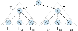
(a) An example of a recursively balance tree $T$ rooted at $v_{1}$. The two subtrees $T_{1}$ and $T_{2}$ of $v_{1}$ are highlighted by larger enclosing triangles.

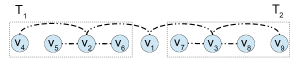
(b) An OLA $\varphi^{*}$ for tree $T$.

Figure 3: An example of a recursively balance tree and it’s corresponding OLA.

Following the results of lemmas 4.5 and 4.6, In following we present an approach to find an OLA for recursively balanced tree in linear time.

Theorem 4.8.

Having a recursively balanced tree $T=(V,E)$ rooted at $v_{r}$, an OLA $\varphi^{*}$ for $T$ can be found in linear time.

Proof.

Assume $T_{r,1},\ldots,T_{r,k}$ are the subtrees connected to $v_{r}$ respectively via $v_{r,1},v_{r,2},\ldots,v_{r,k}\in V$. From lemma 4.5 an OLA $\varphi^{*}$ of type $(T_{r,1},\ldots,T_{r,\overline{k}},v_{r},T_{r,\overline{k}+1},\ldots,T_{k})$ exists for $T$. Each subtree has exactly $\frac{|V|-1}{k}$ vertices, hence $\varphi^{*}(v_{r})=\overline{k}\times\frac{|V|-1}{k}+1$, where $\overline{k}=\lceil\frac{k+1}{2}\rceil$.

Also based on the definition 4.1 every subtree $T_{r,i}$, for $1\leq i\leq k$, is recursively balance with the central vertex $v_{r,i}$. Therefore, using the same approach one can go on with constructing OLA $\varphi^{*}$ by finding the label of $v_{r,i}$, for $1\leq i\leq k$. Applying this method recursively OLA $\varphi^{*}$ can be found while every vertex of the tree is visited $O(1)$ times. ∎

The following two theorems conclude this section by presenting some classes of Halin graphs which there exists a polynomial OLA algorithm for them. More specifically, given a Halin graph $H=T\uplus C$ from these classes, an OLA for $H$ can be derived given any optimal layout for the underlying tree $T$ .

Theorem 4.9.

Consider a Halin graph $H=T\uplus C$, where the underlying tree $T$ is recursively balanced, rooted at $v_{r}$. Let $\varphi^{\circledast}$ be an OLA for $T$. There exist a linear arrangement $\varphi^{*}$ s.t.

• $LA(\varphi^{*},H)=LA(\varphi^{\circledast},T)+2\times(|V|-1)$. Hence, based on corollary 3.7, $\varphi^{*}$ is an OLA for $H$

• $\varphi^{*}$ can be constructed from $\varphi^{\circledast}$ in $O(|V|\log{|V|})$

Proof.

We know that for every layout $\varphi$, it is the case that $LA(\varphi,C)\geq 2\times(n-1)$, where $n=|V|$. Hence, given the OLA $\varphi^{\circledast}$ for $T$, if $LA(\varphi^{\circledast},H)=LA(\varphi^{\circledast},T)+2\times(n-1)$, then $\varphi^{\circledast}$ is also an OLA for $H$ as well. Otherwise, starting from $\varphi^{\circledast}$, we present an iterative approach where using a sequence of swapping operations, an OLA is found for $H$. In this sequence of swapping, after each swap operation the value of arrangement stays unchanged for $T$, and decreases for $H$.

This procedure is presented in algorithm 1. Assume the underlying tree $T$, rooted at central vertex $v_{r}$, has height $\hbar$

Algorithm 1 Finding OLA $\varphi^{*}$ for Halin graph $H=(T,C)$ given OLA $\varphi^{\circledast}$ for RBT $T$

1:$\varphi^{*}\leftarrow\varphi^{\circledast}$

2:let $\{T_{1},\ldots,T_{k}\}$ be subtree of height $\hbar-1$ as $\varphi^{*}$ is of type $(T_{1},\ldots,v_{r},\ldots,T_{k})$

3:let $T_{L}$ be $T_{1}$

4:let $T_{R}$ be one of the two subtrees connected to $T_{L}$ via $E(C)$

5:$\sigma(\varphi^{*},T_{R},T_{k})$

6:for $i=1$ to $k-2$

7: Let $T_{i,R}\in\{T_{i+1},\ldots,T_{k-1}\}$ be the subtree connected to $T_{i}$ via and edge in $E(C)$

8: $\sigma(\varphi^{*},T_{i+1},T_{i,R})$

9:

10:for $h=\hbar$ to $2$:

11: for every subtree $T$ of height $h$ rooted at $v_{r}$:

12:  Let $(T_{r,1},\ldots,v_{r},\ldots,T_{r,k})$ be $\varphi^{*}$ restricted to $T$

13:  if $\varphi^{*}$ is of type $(T,\ldots)$:

14:   ReArrLeftSubTree($(T_{r,1},\ldots,T_{r,k})$, $\varphi^{*}$)

15:  else if $\varphi^{*}$ is of type $(\ldots,T)$:

16:   ReArrRightSubTree($(T_{r,1},\ldots,T_{r,k})$, $\varphi^{*}$)

17:  else:

18:   ReArrMidSubTree($(T_{r,1},\ldots,T_{r,k})$, $\varphi^{*}$)

19:

20:ReArrMidSubTree($(T_{r,1},\ldots,T_{r,k})$, $\varphi^{*}$):

21: Let $T_{r,L}$ be the subtree connected to some vertex $v_{L}$, where based on $\varphi^{*}$, $v_{L}$ is labeled before $T_{r,1}$ Hence, $v_{L}\notin\{V(T_{r,1})\uplus\ldots,\uplus T_{r,k}\}$ and $\forall vin\{V(T_{r,1})\uplus\ldots,\uplus T_{r,k}\},\varphi^{*}(v_{L})<\varphi^{*}(v)$

22: Let $T_{r,R}$ be the subtree connected to some vertex $v_{R}$, where based on $\varphi^{*}$, $v_{R}$ is labeled after $T_{r,k}$ Hence, $v_{R}\notin\{V(T_{r,1})\uplus\ldots,\uplus T_{r,k}\}$ and $\forall vin\{V(T_{r,1})\uplus\ldots,\uplus T_{r,k}\},\varphi^{*}(v)<\varphi^{*}(v_{R})$

23: $\sigma(\varphi^{*},T_{r,1},T_{r,L})$

24: $\sigma(\varphi^{*},T_{r,k},T_{r,R})$

25: if $k>3$:

26:  ReArrMidSubTree($(T_{r,2},\ldots,T_{r,k-1})$, $\varphi^{*}$)

27:

28:ReArrLeftSubTree($(T_{r,1},\ldots,T_{r,k})$, $\varphi^{*}$):

29: Let $T_{r,L}$ be the subtree connected to $T_{R}$ via $E(C)$

30: $\sigma(\varphi^{*},T_{r,1},T_{r,L})$

31: for $i=1$ to $k-2$

32:  Let $T_{i,R}\in\{T_{i+1},\ldots,T_{k}\}$ be the subtree connected to $T_{i}$

33:  $\sigma(\varphi^{*},T_{i+1},T_{i,R})$

34:

35:ReArrRightSubTree($(T_{r,1},\ldots,T_{r,k})$, $\varphi^{*}$):

36: Let $T_{r,R}$ be the subtree connected to $T_{L}$ via $E(C)$

37: $\sigma(\varphi^{*},T_{r,k},T_{r,R})$

38: for $i=k$ to $2$

39:  Let $T_{i,R}\in\{T_{1},\ldots,T_{i-1}\}$ be the subtree connected to $T_{i}$

40:  $\sigma(\varphi^{*},T_{i-1},T_{i,R})$

Correctness of the algorithm.

Starting with $\varphi^{*}=\varphi^{\circledast}$, after execution of line 8, we will end up with a potentially modified layout $\varphi^{*}$ of type $(T_{1},\ldots,v_{r},\ldots,T_{k})$ where $T_{1}$ is directly connected to $T_{k}$ via an edge from $E(C)$ and for $1\leq i<k$, $T_{i}$ is directly connected to $T_{i+1}$ through $E(C)$. So if we collapse every subtree $T_{i}$ for $1\leq i<k$ into one vertex, the resulted $\varphi^{*}$ is an OLA for the corresponding Halin graph.

So far, Based on the resulted layout $\varphi^{*}$, $T_{L}=T_{1}$ and $T_{R}=T_{k}$, respectively defined in lines 3 and 4, are the two left and right boundary subtrees and all other subtrees are middle subtrees.

Lines 10 to 18 of algorithm, guarantee that in a recursive approach, for every subtree $T$ of height $1\leq h<\hbar$, based on the final $\varphi^{*}$ :

• If $T$ is a left side subtree (i.e. if $\varphi^{*}$ is of type $(T,\ldots)$), consider $v\in V(T)$, where $\varphi^{*}(v)=1$. $v$ is connected to $T_{R}$ via $e\in E(C)$

• If $T$ is a right side subtree (i.e. if $\varphi^{*}$ is of type $(\ldots,T)$), consider $v\in V(T)$, where $\varphi^{*}(v)=|V|$. $v$ is connected to $T_{L}$ via $e\in E(C)$

• Otherwise $\varphi^{*}$ is of type $(\ldots,T_{1},T,T_{2},\ldots)$. Let $v_{L}\in V(T)$ be the vertex of $V$ s.t. $\forall v\in V(T),\varphi^{*}(v_{L})\leq\varphi^{*}(v)$. Similarly let $v_{R}\in V(T)$ be the vertex s.t. $\forall v\in V(T),\varphi^{*}(v)\leq\varphi^{*}(v_{R})$. Then $v_{L}$ and $v_{R}$ are respectively directly connected to $T_{1}$ and $T_{2}$ through $E(C)$

Therefore it can be inferred that based on the final layout $\varphi^{*}$, $LA(\varphi^{*},H)=LA(\varphi^{*},T)+LA(\varphi^{*},C)=LA(\varphi^{*},T)+2\times(n-1)$. But we know that the swap operation $\sigma$ does not change the value of linear arrangement for the underlying tree $T$. Hence $LA(\varphi^{*},H)=LA(\varphi^{\circledast},T)+2\times(n-1)$ which induces the optimality of $\varphi^{*}$.

Time complexity analysis.

The time complexity of the algorithm depends on the two major For loops in lines 6 and 10.

• Analysis of the first loop in line 6. Assuming every basic swap operation is an atomic operation with cost $O(1)$, then the cost of every $\sigma(\varphi^{*},T_{1},T_{2})$ is $O(|V(T_{1})|)=O(|V(T_{2})|)$. Hence, the cost of the loop at line 6 is $O(k\times\dfrac{n-1}{k})=O(n)$ .

• Analysis of the second loop in line 10. At every iteration, if there are $k$ subtrees $\{T_{r,1},\ldots,T_{r,k}\}$, In worst-case scenario at most $O(k)$ swap operations $\sigma$ are carried out. For $1\leq i\leq k$, $|V(T_{r,i})|=\dfrac{n}{k}$ .Therefore the cost of each iteration is $O(k\times\dfrac{n}{k})=O(n)$.

  Having the fact that $\hbar=O(\log{n})$, we conclude the time complexity of the loop in line 10 as $O(n\log{n})$, which dominates the time complexity of the whole algorithm.

∎

Example 4.10.

In figure 3, two layouts are presented for the Halin graph $H_{2}=T\uplus C$ (Figure 2(a) in section 2). Layout $\varphi_{1}$ in Figure 4(a), is an OLA for the underlying tree of graph $H_{2}$ while it is not an optimal layout for $H_{2}$ itself (the OLA for $H_{2}$ is shown in Figure 4(b)). Enumerating all the OLAs for the underlying tree of $H_{2}$, it can be verified that non is an OLA for $H_{2}$.

$P=(v_{7},v_{2},v_{2},v_{4},v_{12})$ is the spinal path corresponding to the layout $\varphi_{1}$. After removing the edges of the spinal path $P$ and cycle $C$, each vertex $v_{i}$ of the path $P$ corresponds to a subtree $T_{i}$. Notice that subtree $T_{1}$, rooted at $v_{1}$, is not an RBT. Hence based on the order of arrangement of the three branches connected to $v_{1}$, we may get different values for the linear arrangement, and an ordering of the branches with the optimal arrangement values for $T$, is not necessary optimal after adding the edge of cycle $C$ and path $P$ back.

As opposed to the OLA of the underlying tree of $H_{2}$, given an OLA $\varphi$ for an arbitrary RBT $T^{\prime}$, and an arbitrary subtree $T_{i}$ rooted at some spinal vertex $v_{i}$, all the branches of $T_{i}$ connected to $v_{i}$ have the same number of vertices and are also recursively balanced. Hence for every Halin graph $H^{\prime}=T^{\prime}\uplus C^{\prime}$ based on $T^{\prime}$, the layout $\varphi$ can be modified by changing the order of the branches of the subtrees where the value of linear arrangement for $T^{\prime}$ stays unchanged (Let’s call the modified layout $\varphi^{\prime}$), while the value of linear arrangement for the edges of cycle $C^{\prime}$ (i.e. $\sum_{\{v,u\}\in E(C^{\prime})}\lambda(\{v,u\},\varphi^{\prime})$) is equal to $2\times(n-1)$ . Consequently the value of OLA for $H^{\prime}$ is equal to $LA(\varphi,T)+2\times(n-1)$. $\square$

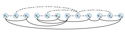
(a) Layout $\varphi_{1}$ is an OLA for underlying tree of Halin graph $H_{2}$.

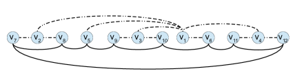
(b) Layout $\varphi_{2}$ is an OLA for Halin graph $H_{2}$.

Figure 4: Two layout $\varphi_{1}$ and $\varphi_{2}$ for Halin graph $H_{2}=T\uplus C$ (Figure 2(a) in section 2), where $LA(\varphi_{1},H_{2})>LA(\varphi_{2},H_{2})$ while $LA(\varphi_{1},T)<LA(\varphi_{2},T)$. More specifically $\varphi_{1}$ is an OLA for $T$ and $\varphi_{2}$ is the OLA for $H_{2}$.

Corollary 4.11.

Let $T$ be the underlying tree for some Halin graph $H=T\uplus C$ and let $\varphi^{\circledast}$ be an OLA for $T$ where $P=(w_{1},\ldots,w_{l})$ is respectively the spinal path and based on $\varphi^{\circledast}$, and $\{T_{1},\ldots,T_{l}\}$ is the set of subtrees remaining after removing all edges of $C$ and $P$.

If for some OLA $\varphi^{\circledast}$ of $T$, $T_{i}$ rooted at $w_{i}$ is a recursively balance tree for $i=1,\ldots,l$, then there exists an OLA $\varphi^{*}$ for $H$ where $LA(\varphi^{*},H)=LA(\varphi^{\circledast},T)+2\times(n-1)$.

Another class of Halin graphs which their underlying trees satisfy the sufficient property of corollary 4.11, are the Halin graphs based on caterpillar trees. This class of Halin graphs is studied in [3] and presented result on value of their OLA, testifies the corollary 4.11.

5 Conclusion and Future Work

As one of the simplest classes of non-outerplanar graphs, in this work we studied some properties of OLA of Halin graphs and we presented a lower bound for the value of OLA for Halin graphs. We also introduced some classes of Halin graphs which the OLA can be found in $O(n\log{n})$. The problem of OLA of general Halin graphs is still open and we believe a solution for the OLA of general Halin graphs gives good insights into the properties of OLA of the more general class of k-outerplanar graphs.

Appendix A Appendix: Proofs of Supporting Lemmas for Section 3

Notation A.1.

Consider the layout $\varphi$ for a Halin graph $H=T\uplus C$ and it’s corresponding spinal path $P=(w_{1},w_{2},\dots,w_{l})$. $\mathcal{T}_{i}=|\{u\text{ s.t. }u\in V(T_{i})\}|$ presents the number of vertices of an spinal subtree $T_{i}$. Similarly for branch $B_{i,j}$, $\beta_{i,j}=|\{u\text{ s.t. }u\in V(B_{i,j})\}|$ stands for the number of vertices of branch $B_{i,j}$.

Notation A.2.

Given vertex $v\in V$, subset $\mathcal{V}\subseteq V$ and a layout $\varphi$, we define:

$$\delta_{\varphi}(\underline{v},\overline{v},\mathcal{V})= |\{u\text{ s.t. }u\in\mathcal{V}\text{ and }\varphi(\underline{v})<\varphi(u)<\varphi(\overline{u})\}|$$

In other word, $\delta_{\varphi}(\underline{v},\overline{v},\mathcal{V})$ is the number of vertices in $\mathcal{V}$, which based on $\varphi$ are labeled with integers greater than the label of $\underline{v}$ and smaller than the label of $\overline{v}$. Respectively $\delta_{\varphi}(-,\overline{v},\mathcal{V})$ and $\delta_{\varphi}(\underline{v},-,\mathcal{V})$ can be interpreted as the number of vertices of $\mathcal{V}$ labeled before $\overline{v}$ and after $\underline{v}$.

In what follows we present an auxiliary lemma and its proof that will be helpful in simplifying and understanding of the proof of lemma 3.3.

Lemma A.3.

Consider the OLA $\varphi^{*}$ for the Halin graph $H=T\uplus C$ and the corresponding spinal path $P=(w_{1},w_{2},\dots,w_{l})$. Removing all the edges of $P$ and $C$ results in a set of $l$ subtrees $T_{1},\ldots,T_{l}$ respectively rooted at $w_{1},\ldots,w_{l}$. In the layout $\varphi^{*}$, the vertices of $T_{1}$ are labeled by contentious integers and before all the vertices of $H-T_{1}$. Formally speaking:

$$\forall v\in T_{1},u\notin T_{1}\Rightarrow\varphi^{*}(v)<\varphi^{*}(u)$$

Proof.

We prove this lemma by showing that the opposing assumption contradicts the optimality of $\varphi^{*}$. In other other word, if $\exists v\in V(T_{1}),u\notin V(T_{1}),\varphi^{*}(u)<\varphi^{*}(v)$, we suggest an alternative layout $\varphi^{\diamond}$ where $LA(\varphi^{*},H)>LA(\varphi^{\diamond},H)$. Two layouts $\varphi^{*}$ and $\varphi^{\diamond}$ are respectively shown in Figure 5(a) and 5(b).

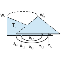
(a) OLA layout $\varphi^{*}$ which labels some vertex $u\in V(T_{1})$ with integers larger than the label of some vertex $v\in V(H)-V(T_{1})$. In other word the arrangement of $T_{1}$ has overlapping area with arrangement of $H-T_{1}$.

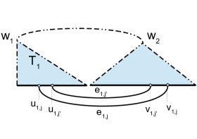
(b) In the layout $\varphi^{\diamond}$ all the vertices of $T_{1}$ are labeled before the vertices of $H-T_{1}$.

Figure 5: The OLA $\varphi^{*}$ and the alternative layout $\varphi^{\diamond}$.

In layout $\varphi^{\diamond}$, defined as it follows, all the vertices of $T_{1}$ are labeled with integers smaller than all the labels of vertices in $V(H)-V(T_{1})$ by shifting them to the left while keeping their relative orders unchanged.

$$\forall v\in V,\varphi^{\diamond}=\begin{cases}\varphi^{*}(v)-\delta_{\varphi^{*}}(-,v,V(H)-V(T_{1}))&\quad\text{if }v\in V(T_{1})\\ \varphi^{*}(v)+\delta_{\varphi^{*}}(v,-,V(T_{1}))&\quad\text{if }v\notin V(T_{1})\end{cases}$$

Going from layout $\varphi^{*}$ to $\varphi^{\diamond}$, the equation 1 can be inferred.

(1) $$LA(\varphi^{*},H)-LA(\varphi^{\diamond},H)=$$

$$\Delta+$$

$$\lambda(\{w_{1},w_{2}\},\varphi^{*})-\lambda(\{w_{1},w_{2}\},\varphi^{\diamond})+$$

$$\lambda(e_{1,j},\varphi^{*})-\lambda(e_{1,j},\varphi^{\diamond})+$$

$$\lambda(e_{1,j^{\prime}},\varphi^{*})-\lambda(e_{1,j^{\prime}},\varphi^{\diamond})+$$

Where $\Delta$ is the increase in the value of linear arrangement due to overlapping vertices.

Value of $\Delta$:

We define $\Delta_{1}$ and $\Delta_{2}$ respectively as the number of vertices of $V(T_{1})$ and $V(H)-V(T_{1})$ in the overlapping area. More specifically:

$$\Delta_{1}=|\{v\in V(T_{1})\text{ s.t. }\exists u,u^{\prime}\in V(H)-V(T_{1}),\varphi^{*}(u)<\varphi^{*}(v)<\varphi^{*}(u^{\prime})\}|$$

$$\Delta_{2}=|\{v\in V(H)-V(T_{1})\text{ s.t. }\exists u,u^{\prime}\in V(T_{1}),\varphi^{*}(u)<\varphi^{*}(v)<\varphi^{*}(u^{\prime})\}|$$

Fact A.4.

As presented in Figure 5, the set of vertices $V(T_{1})$ and $V(H)-V(T_{1})$ are connected via exactly three outgoing edges $\{w_{1},w_{2}\}$, $e_{1,j}$ and $e_{1,j^{\prime}}$. Based on the three-connectivity of Halin graphs, any subset $\mathcal{V}\subset V(T_{1})$ not incident to the outgoing edges, is connected to the rest of $V(T_{1})$ by at least three edge disjoint paths. Also Any subset $\mathcal{V}\subset V(T_{1})$ incident to some of outgoing edges $\{w_{1},w_{2}\}$, $e_{1,j}$ and $e_{1,j^{\prime}}$, is connected to $V(T_{1})-\mathcal{V}$ via at least two edge-disjoint paths. the same property hold for any $\mathcal{V}\subset V(H)-V(T_{1})$.

According to fact A.4, any vertex $v\in V(T_{1})$ in the overlapping area participates one unit in increasing the expand of at least two edges of $E(H/T_{1})$. Similarly any vertex $v\in V(H)-V(T_{1})$ in overlapping area, increases the expand of at least two edges from $E(T_{1})$. Hence:

(2) $$\Delta\geq 2\times(\Delta_{1}+\Delta_{2})$$

Change in the expands of $\{w_{1},w_{2}\}$, $e_{1,j}$ and $e_{2,j^{\prime}}$:

Based on the procedure that $\varphi^{\diamond}$ is constructed from $\varphi^{*}$ it’s easy to validate the following equations.

(3) $$(\lambda(\{w_{1},w_{2}\},\varphi^{*})-\lambda(\{w_{1},w_{2}\},\varphi^{\diamond}))=-\delta(w_{2},-,V(T_{1}))\geq-\Delta_{1}$$

(4) $$(\lambda(e_{1,j},\varphi^{*})-\lambda(e_{1,j},\varphi^{\diamond}))=-(\delta(-,u_{1,j},V(H)-V(T_{1}))+\delta(v_{1,j},-,V(T_{1})))>-(\Delta_{2}+\Delta_{1})$$

(5) $$(\lambda(e_{1,j^{\prime}},\varphi^{*})-\lambda(e_{1,j^{\prime}},\varphi^{\diamond}))=-(\delta(-,u_{1,j^{\prime}},V(H)-V(T_{1}))+\delta(v_{1,j^{\prime}},-,V(T_{1})))>-(\Delta_{2}+\Delta_{1})$$

Remark A.5.

Let $v\in\{w_{2},v_{1,j},v_{1,j^{\prime}}\}$ be the vertex with largest label among the three. The rearrangement of $v$ increases the expand of the corresponding edges by $\delta(v,-,V(T_{1})))$. But notice that based on fact A.4 the set of vertices of $V(H)-V(T_{1})$ labeled after $v$ are connected to rest of vertices (vertices on left side according to $\varphi^{*}$) using at least three vertices. Hence each vertex of $V(T_{1})$ after $v$ (labeled with integers larger than label of $v$) add one unit to the expands of at least three edges of $H/T_{1}$, while only the expands of two edges where considered in equation 2. Therefore the value $\delta(v,-,V(T_{1}))$ in the increase of the expand of the edge incident to $v$ must be ignored in the calculation of $LA(\varphi^{*},H)-LA(\varphi^{\diamond},H)$.

Considering the remark  A.8, we finalize the proof by the following contradictory result.

(6) $$LA(\varphi^{*},H)-LA(\varphi^{\diamond},H)>$$

(7) $$2\times(\Delta_{1}+\Delta_{2})-\Delta_{1}-(\Delta_{2}+\Delta_{1})-\Delta_{2}$$

(8) $$>0$$

∎

Proof A.6.

(Proof of lemma 3.3) In lemma A.3, it is shown that, given an OLA $\varphi^{*}$ for the Halin graph $H$, all the vertices of $T_{1}$ are labeled with continuous integers and hence are arranged before all other vertices in the graph. Using a similar approach as in lemma A.3, we show that in an OLA $\varphi^{*}$ all the vertices in $V(T_{2})$ are labeled before all the vertices of $V(T_{3})\cup\ldots\cup V(T_{l})$. Proof is complete as the same approach can be carried out to show that $\forall 2<i<l$ all the vertices of $V(T_{i})$ are labeled with integers smaller than the labels of vertices of $V(T_{i+1})\cup\ldots\cup V(T_{l})$.

In the rest of this proof we present $T_{3}\uplus\ldots\uplus T_{l}$ by $\overline{T}_{1,2}$. We show that a layout $\varphi^{*}$, where the arrangement of vertices of $T_{2}$ overlap with the arrangement of vertices in $V(\overline{T}_{1,2})$ (as shown in Figure 6(a)) cannot be optimal. In order to do so, based on this allegedly optimal layout $\varphi^{*}$, we define the modified layout $\varphi^{\diamond}$ (presented by Figure 6(b)) and we show that $LA(\varphi^{*})>LA(\varphi^{\diamond})$.

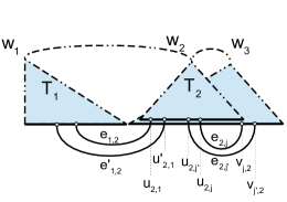
(a) OLA layout $\varphi^{*}$ which labels some vertex $u\in V(T_{2})$ with integers larger than the label of some vertex $v\in V(\overline{T}_{1,2})$. In other word the arrangement of $T_{2}$ has overlapping area with arrangement of $T_{3}\uplus\ldots\uplus T_{l}$.

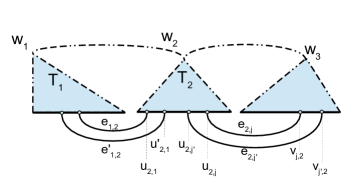
(b) In the layout $\varphi^{\diamond}$ all the vertices of $T_{2}$ are labeled after the vertices of $T_{1}$ and before all the vertices of $V(\overline{T}_{1,2})$.

Figure 6: The OLA $\varphi^{*}$ and the alternative layout $\varphi^{\diamond}$. Subtree $T_{2}$ is connected to $T_{1}$ via at most two edges $e_{1,2},e^{\prime}_{1,2}\in E(C)$, (respectively incident to $u_{1,2},u^{\prime}_{1,2}\in V(T_{2})$) and exactly one edge $\{w_{1},w_{2}\}\in E(T)$. $T_{2}$ is also connected to the rest of graph by the same number of edges0 $e_{2,j},e_{2,j^{\prime}}\in E(C)$ and $\{w_{2},w_{3}\}$. End points of edge $e_{2,j}$ are $u_{2,j}\in V(T_{2})$ and $v_{2,j}\in V(\overline{T}_{1,2})$ while $u_{2,j^{\prime}}\in V(T_{2})$ and $v_{2,j^{\prime}}\in V(\overline{T}_{1,2})$ are the two end points of $e_{2,j^{\prime}}$.

The subtree $T_{2}$ is connected to $T_{1}$ through one edge $e_{1,2}\in E(T)$ and one or two edges from $E(C)$. $T_{2}$ is also connected to the rest of graph by exactly the same number of edges. As presented in Figure 6, we only consider the case where $T_{2}$ is connected to each of subgraphs $T_{2}$ and $T_{3}\uplus\ldots\uplus T_{l}$ by one edge of $E(T)$ and two edges of $E(C)$. The other case can be analyze in the same way and is omitted.

Layout $\varphi^{\diamond}$ is formally defined as it follows.

$$\forall v\in V,\varphi^{\diamond}=\begin{cases}\varphi^{*}(v)-\delta_{\varphi^{*}}(-,v,V(\overline{T}_{1,2}))&\quad\text{if }v\in V(T_{2})\\ \varphi^{*}(v)+\delta_{\varphi^{*}}(v,-,V(T_{2}))&\quad\text{if }v\in V(\overline{T}_{1,2})\end{cases}$$

Based on this definition it’s easy to see that:

(9) $$LA(\varphi^{*},H)-LA(\varphi^{\diamond},H)=$$

$$\Delta+$$

$$(\lambda(\{w_{1},w_{2}\},\varphi^{*})-\lambda(\{w_{1},w_{2}\},\varphi^{\diamond}))+$$

$$(\lambda(\{w_{2},w_{3}\},\varphi^{*})-\lambda(\{w_{2},w_{3}\},\varphi^{\diamond}))+$$

$$(\lambda(e_{1,2},\varphi^{*})-\lambda(e_{1,2},\varphi^{\diamond}))+$$

$$(\lambda(e^{\prime}_{1,2},\varphi^{*})-\lambda(e^{\prime}_{1,2},\varphi^{\diamond}))+$$

$$(\lambda(e_{2,j},\varphi^{*})-\lambda(e_{2,j},\varphi^{\diamond}))+$$

$$(\lambda(e_{2,j^{\prime}},\varphi^{*})-\lambda(e_{2,j^{\prime}},\varphi^{\diamond}))+$$

As in lemma A.3 the increase in the value of linear arrangement due to overlap is presented by $\Delta$ and we define $\Delta_{2}$ and $\Delta_{3}$ as:

$$\Delta_{2}=|\{v\in V(T_{2})\text{ s.t. }\exists u,u^{\prime}\in V(\overline{T}_{1,2}),\varphi^{*}(u)<\varphi^{*}(v)<\varphi^{*}(u^{\prime})\}|$$

$$\Delta_{3}=|\{v\in V(\overline{T}_{1,2})\text{ s.t. }\exists u,u^{\prime}\in V(T_{2}),\varphi^{*}(u)<\varphi^{*}(v)<\varphi^{*}(u^{\prime})\}|$$

Hence $\Delta_{2}$ and $\Delta_{3}$ respectively correspond to the number of vertices of $T_{2}$ and $T_{3}\uplus\ldots\uplus T_{l}$ which are in the overlapping area based on $\varphi^{*}$.

Fact A.7.

Similar to the fact A.4 and according to the three-connectivity of Halin graphs, any subset $\mathcal{V}\subset V(\overline{T}_{1,2})$ not incident to the outgoing edges $\{w_{2},w_{3}\}$, $e_{2,j}$ and $e_{2,j^{\prime}}$, is connected to the rest of $V(\overline{T}_{1,2})$ through at least three edge disjoint paths. Also Any subset $\mathcal{V}\subset V(\overline{T}_{1,2})$ incident to some of the outgoing edges, is connected to $V(\overline{T}_{1,2})-\mathcal{V}$ via at least two edge-disjoint paths. The same property hold for any $\mathcal{V}\subset V(T_{1})\cup V(T_{2})$.

Value of $\Delta$:

Using the fact A.7 one can see that each vertex in the overlapping area, increases the expand of at least two edges by one unit. Hence the following equation can be deduced.

(10) $$\Delta\geq 2\times(\Delta_{2}+\Delta_{3})$$

Change in the expands of outgoing edges:

As in lemma A.3, the change in the expand of edges linking $T_{2}$ to the rest of graph can be derived as:

(11) $$(\lambda(\{w_{1},w_{2}\},\varphi^{*})-\lambda(\{w_{1},w_{2}\},\varphi^{\diamond}))=\delta(-,w_{2},V(\overline{T}_{1,2}))$$

(12) $$(\lambda(\{w_{2},w_{3}\},\varphi^{*})-\lambda(\{w_{2},w_{3}\},\varphi^{\diamond}))=-(\delta(-,w_{2},V(\overline{T}_{1,2}))+\delta(w_{3},-,V(T_{2})))$$

(13) $$(\lambda(e_{1,2},\varphi^{*})-\lambda(e_{1,2},\varphi^{\diamond}))=\delta(-,u_{1,2},V(\overline{T}_{1,2}))$$

(14) $$(\lambda(e^{\prime}_{1,2},\varphi^{*})-\lambda(e^{\prime}_{1,2},\varphi^{\diamond}))=\delta(-,u^{\prime}_{1,2},V(\overline{T}_{1,2}))$$

(15) $$(\lambda(e_{2,j},\varphi^{*})-\lambda(e_{2,j},\varphi^{\diamond}))\geq-(\delta(-,u_{2,j},V(\overline{T}_{1,2}))+\delta(v_{j,2},-,V(T_{2})))$$

(16) $$(\lambda(e_{2,j^{\prime}},\varphi^{*})-\lambda(e_{2,j^{\prime}},\varphi^{\diamond}))\geq-(\delta(-,u_{2,j^{\prime}},V(\overline{T}_{1,2}))+\delta(v_{j^{\prime},2},-,V(T_{2})))$$

Remark A.8.

Let $v\in\{w_{3},v_{j,2},v_{j^{\prime},2}\}$ be the vertex with largest label among the three. According to the fact A.7 and using the same reasoning as in remark A.8, each vertex in $V(T_{2})$ labeled after $v$ takes part in the increase of expand of at least three edges of $V(\overline{T}_{1,2})$, while only two where considered in the calculation of $\Delta$ in equation 10. Hence the value $\delta(v,-,V(T_{2}))$, considered for the change in expand of the edge incident to $v$, should be added back to the calculation of $LA(\varphi^{*},H)-LA(\varphi^{\diamond},H)$. Without loss of generality in the rest of the proof we assume $v=v_{j^{\prime},2}$.

Accordingly equation 9 can be simplified as it follows.

(17) $$LA(\varphi^{*},H)-LA(\varphi^{\diamond},H)\geq$$

$$2\times(\Delta_{2}+\Delta_{3})$$

$$-\delta(w_{3},-,V(T_{2}))$$

$$-\delta(u_{1,2},u_{2,j},V(\overline{T}_{1,2}))$$

$$-\delta(u^{\prime}_{1,2},u_{2,j^{\prime}},V(\overline{T}_{1,2}))$$

(18) $$-\delta(v_{j,2},-,V(T_{1,2}))$$

Remark A.9.

Depending on the order of labels of $u_{1,2}$ and $u_{2,j}$, $\delta(-,u_{1,2},V(\overline{T}_{1,2}))-\delta(-,u_{2,j},V(\overline{T}_{1,2}))$ is either equal to $\delta(u_{2,j},u_{1,2},V(\overline{T}_{1,2}))$ or $-\delta(u_{1,2},u_{2,j},V(\overline{T}_{1,2}))$. The same way we can reason about $\delta(-,u^{\prime}_{1,2},V(\overline{T}_{1,2}))-\delta(-,u_{2,j^{\prime}},V(\overline{T}_{1,2}))$ as following:

(19) $$\delta(-,u_{1,2},V(\overline{T}_{1,2}))-\delta(-,u_{2,j},V(\overline{T}_{1,2}))\geq -\delta(u_{1,2},u_{2,j},V(\overline{T}_{1,2}))\geq-\Delta_{3}$$

(20) $$\delta(-,u^{\prime}_{1,2},V(\overline{T}_{1,2}))-\delta(-,u_{2,j^{\prime}},V(\overline{T}_{1,2}))\geq -\delta(u^{\prime}_{1,2},u_{2,j^{\prime}},V(\overline{T}_{1,2}))\geq-\Delta_{3}$$

Also it is easy to see that:

(21) $$-\delta(w_{3},-,V(T_{2}))\geq\Delta_{2}$$

(22) $$-\delta(v_{2,j},-,V(T_{1,2}))\geq\Delta_{2}$$

Remark A.10.

The equality in equation 15 holds only if $u_{2,j}$ is labeled before $v_{j,2}$ (namely $\varphi^{*}(u_{2,j})<\varphi^{*}(v_{2,j})$) . But the equalities in equations 19 and 22 can hold simultaneously only if $v_{2,j}$ is labeled before all the vertices $V(T_{2})$ in the overlapping area and $u_{2,j}$ is labeled after all the vertices of $\overline{T}_{1,2}$ which are in the overlapping area. In other word, both the equalities in equations19 and 22 hold only if $\varphi^{*}(u_{2,j})>\varphi^{*}(v_{2,j})$. Accordingly the equalities in equations 15, 19 and 22 never simultaneously hold.

Consequently the equation 17 can be simplified as following with the contradictory result that completes the proof.

(23) $$LA(\varphi^{*},H)-LA(\varphi^{\diamond},H)>$$

$$2\times(\Delta_{2}+\Delta_{3})$$

$$-\Delta_{2}$$

$$-\Delta_{3}$$

$$-\Delta_{3}$$

(24) $$-\Delta_{2}=0$$

Proof A.11.

(Proof of lemma 3.5) Each spinal branch $B_{i,j}$ is connected to the rest of the graph using three edges. $e_{j,w}=\{v_{j},w_{i}\}\in E(T)$ connecting it to the spinal vertex $w_{i}$ and two edge $e_{j,j^{\prime}}\in E(C)$ and $e_{j,j^{\prime\prime}}\in E(C)$ connecting $B_{i,j}$ to two other branches $B_{i^{\prime},j^{\prime}}$ and $B_{i^{\prime\prime},j^{\prime\prime}}$ .

Without loss of generality we assume $j=1$ and $j^{\prime}=2$ and we consider two branches $B_{i,1}$ and $B_{i,2}$ are anchored at $v_{1}$ and $v_{2}$, and we only show the following for the case where $\varphi^{*}$ is of type $(\ldots,w_{i},\ldots,V(B_{i,1})\cup V(B_{i,2}),\ldots)$.

$$\forall v\in V(B_{i,1})\cup V(B_{i,2});\varphi^{*}(w_{i})<\varphi^{*}(v)\Rightarrow$$

$$(\forall v\in V(B_{i,1}),u\in V(B_{i,2}):\varphi^{*}(v)<\varphi^{*}(u))\vee$$

$$(\forall v\in V(B_{i,1}),u\in V(B_{i,2}):\varphi^{*}(v)>\varphi^{*}(u))$$

Assume two vertices $\underline{v},\overline{v}\in V(B_{i,1})\cup V(B_{i,2})$ such that $\forall u\in V(B_{i,1})\cup V(B_{i,2}),\varphi^{*}(\underline{v})\leq u\leq\varphi^{*}(\overline{v})$.

Case 1: $\underline{v}\in B_{i,1}$ and $\overline{v}\in B_{i,2}$.

There are two possible sub-cases: 1.1) there is no edge connecting $B_{i,1}$ and $B_{i,2}$. 1.2) $B_{i,1}$ is connected to $B_{i,2}$ using exactly one edge $e_{1,2}\in E(C)$ (Figure 7). We present the proof for the later case. The analysis of proof of former case is similar and omitted. We show that the assumption of lemma being false, in other word if two branches of $B_{i,1}$ and $B_{i,1}$ overlap, contradicts the optimality assumption of $\varphi^{*}$. Accordingly for an overlapping OLA $\varphi^{*}$, we present an alternative layout $\varphi^{\diamond}_{L}$ and finish the proof by showing the contradictory result $LA(\varphi^{*})>LA(\varphi^{\diamond}_{L})$.

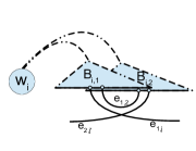
Figure 7: An branch overlapping layout where the two branches $B_{i,1}$ and $B_{i,2}$ are connected.

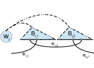
(a) The alternative non-overlapping layout $\varphi^{\diamond}_{L}$.

(b) The alternative non-overlapping layout $\varphi^{\diamond}_{R}$.

Figure 8: In the layout $\varphi^{\diamond}_{L}$ all the vertices of $B_{i,1}$ are labeled on the left side of vertices of $B_{i,2}$ and on the right side in the layout $\varphi^{\diamond}_{R}$.

In the alternative layout $\varphi^{\diamond}_{L}$ all the vertices of $B_{i,1}$ are labeled before all the vertices of $B_{i,2}$ while the relative order of labels of other vertices are preserved the same. Formally $\varphi^{\diamond}_{L}$ is defined as follows.

$$\forall v\in V,\varphi^{\diamond}_{L}=\begin{cases}\varphi^{*}(v)&\quad\text{if }v\notin V(B_{i,1})\cup V(B_{i,1})\\ \varphi^{*}(v)-\delta_{\varphi^{*}}(-,v,V(B_{i,2}))&\quad\text{if }v\in V(B_{i,1})\\ \varphi^{*}(v)+\delta_{\varphi^{*}}(v,-,V(B_{i,1}))&\quad\text{if }v\in V(B_{i,2})\end{cases}$$

Based on the definition of $\varphi^{\diamond}_{L}$ and from Figure 8(a) the following holds:

(25) $$LA(\varphi^{*})-LA(\varphi^{\diamond}_{L})=$$

$$\Delta+$$

$$(\lambda(e_{1,2},\varphi^{*})-\lambda(e_{1,2},\varphi^{\diamond}_{L}))+$$

$$(\lambda(e_{1,j^{\prime}},\varphi^{*})-\lambda(e_{1,j^{\prime}},\varphi^{\diamond}_{L}))+$$

$$(\lambda(e_{2,j},\varphi^{*})-\lambda(e_{2,j},\varphi^{\diamond}_{L}))+$$

$$(\lambda(e_{1,w},\varphi^{*})-\lambda(e_{1,w},\varphi^{\diamond}_{L}))+$$

$$(\lambda(e_{2,w},\varphi^{*})-\lambda(e_{1,w},\varphi^{\diamond}_{L}))$$

As before, $\Delta$ represents the increase in the value of linear arrangement due to overlap.

Let $\Delta_{1}$ and $\Delta_{2}$ respectively be the number of vertices of $B_{i,1}$ and $B_{i,2}$ in the overlapping area. Formally speaking:

$$\Delta_{1}=|\{v\in B_{i,1}|\exists u,u^{\prime}\in B_{i,2},\varphi^{*}(u)<\varphi^{*}(v)<\varphi^{*}(u^{\prime})\}|$$

$$\Delta_{2}=|\{v\in B_{i,2}|\exists u,u^{\prime}\in B_{i,1},\varphi^{*}(u)<\varphi^{*}(v)<\varphi^{*}(u^{\prime})\}|$$

Fact A.12.

Every spinal branch $B_{i,j}$ of a Halin graph $H=T\uplus C$, anchored at $v_{i,j}$, is connected to the rest of $H$ via three outgoing edges, $\{w_{i},v_{i,j}\}\in E(T)$, $e_{j,j^{\prime}}\in E(C)$ and $e_{j,j^{\prime\prime}}\in E(C)$. The two edges $e_{j,j^{\prime}}$ and $e_{j,j^{\prime\prime}}$, respectively incident to $v_{R}$ and $v_{L}$, connect $B_{i,j}$ to two other spinal branches $B_{i^{\prime},j^{\prime}}$ and $B_{i^{\prime\prime},j^{\prime\prime}}$ . Every vertex of a non-empty sub-branch $\mathcal{B}\subset B_{i,j}-\{v_{i,j},v_{j,R},v_{j,L}\}$ is connected to $B_{i,j}/\mathcal{B}$ via at least three edge disjoint paths. Consequently $\mathcal{B}$ is connected to $B_{i,j}/\mathcal{B}$ by at least three edges.

In general every vertex of a non-empty set $\mathcal{B}\subset B_{i,j}$ (which may contains some of the vertices of $\{v_{i,j},v_{j,R},v_{j,L}\}$) is connected to $B_{i,j}/\mathcal{B}$ by at least two edges-disjoint paths.

Value of $\Delta$:

As a consequence of fact A.12, each vertex of a branch in the overlapping area contribute one unit to the increase in the expand of at least two edges from the other branch. Hence it is the case that:

(26) $$\Delta\geq 2\times(\Delta_{1}+\Delta_{2})$$

Change in the expands of $e_{1,2}$, $e_{1,j^{\prime}}$, $e_{2,j^{\prime\prime}}$ and $e_{2,w}$:

The increase in the expand of each of these edges is equivalent to how much the two end points drift apart in construction of $\varphi^{\diamond}_{L}$. Accordingly the following equations are easy to verify:

(27) $$(\lambda(e_{1,2},\varphi^{*})-\lambda(e_{1,2},\varphi^{\diamond}_{L}))\geq-(\Delta_{1}+\Delta_{2})$$

(28) $$(\lambda(e_{1,j^{\prime}},\varphi^{*})-\lambda(e_{1,j^{\prime}},\varphi^{\diamond}_{L}))\geq-\Delta_{2}$$

(29) $$(\lambda(e_{2,j^{\prime\prime}},\varphi^{*})-\lambda(e_{2,j^{\prime\prime}},\varphi^{\diamond}_{L}))\geq-\Delta_{1}$$

(30) $$(\lambda(e_{2,w},\varphi^{*})-\lambda(e_{2,w},\varphi^{\diamond}_{L}))\geq-\Delta_{1}$$

Remark A.13.

Let $u\in V(B_{i,2})$ be the vertex incident to one of the edges $e_{1,2}$, $e_{2,j^{\prime\prime}}$ and $e_{2,w}$ with the largest label based on $\varphi^{*}$. Using fact A.12, the set of vertices of $\overrightarrow{\mathcal{V}}_{u}\subset V(B_{i,2})$ labeled after $u$ is three-connected to set of vertices labeled before $u$. Accordingly each vertex of $B_{i,1}$ labeled with an integer larger that $\varphi^{*}(u)$ contributes one unit to the increase in expand of at least three edges of $B_{i,2}$. Therefore this value cancels out the expand of the edge incident to $u$.

Remark A.14.

It’s easy to see that at most only one of the equalities 27 to 30 can hold.

The following contradictory result, from putting the equations 26 to 29 and remarks A.13 and A.14 together, concludes our proof in this case.

$$LA(\varphi^{*})-LA(\varphi^{\diamond}_{L})>2\times(\Delta_{1}+\Delta_{2})+-(\Delta_{1}+\Delta_{2})-\Delta_{1}-\Delta_{2}=0$$

Case 2: $\underline{v}\in B_{i,2}$ and $\overline{v}\in B_{i,1}$.

This case is symmetric to the previous case and in the alternative layout $\varphi^{\diamond}_{L}$ all the vertices of $B_{i,1}$ are labeled after those of $B_{i,2}$. Hence the proof is similar and is omitted.

Case 3: $\underline{v},\overline{v}\in B_{i,1}$.

Layout $\varphi^{*}$ for this case is presented in Figure 9 where all the vertices of $B_{i,2}$ are enclosed by $B_{i,1}$. In contrast to layout $\varphi^{*}$, we present layout $\varphi^{\diamond}_{R}$ where all vertices of $B_{i,1}$ are labeled on the right side of those of $B_{i,2}$ as formally defined in following.

$$\forall v\in V,\varphi^{\diamond}_{R}=\begin{cases}\varphi^{*}(v)&\quad\text{if }v\notin V(B_{i,1})\cup V(B_{i,1})\\ \varphi^{*}(v)+\delta_{\varphi^{*}}(v,\overline{v},V(B_{i,2}))&\quad\text{if }v\in V(B_{i,1})\\ \varphi^{*}(v)-\delta_{\varphi^{*}}(w_{i},v,V(B_{i,1}))&\quad\text{if }v\in V(B_{i,2})\end{cases}$$

We finish the proof by showing that either $LA(\varphi^{*})>\varphi^{\diamond}_{R}$ or $LA(\varphi^{*})>\varphi^{\diamond}_{L}$.

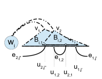
Figure 9: General presentation of an OLA $\varphi^{*}$ where $\underline{v},\overline{v}\in B_{i,1}$. $u_{1,2}\in V(B_{i,1})$ and $u_{2,1}\in V(B_{i,2})$ are the two end points of edge $e_{1,2}$ while $u_{1,j^{\prime}}\in V(B_{i,1})$ and $u_{2,j^{\prime\prime}}\in V(B_{i,2})$ are respectively one of the end points of two edge $e_{1,j^{\prime}}$ and $e_{2,j^{\prime\prime}}$.

According to the definitions of $\varphi^{\diamond}_{R}$ and $\varphi^{\diamond}_{L}$ one can inferred the equation 31.

(31) $$LA(\varphi^{*})-LA(\varphi^{\diamond}_{-})=$$

$$\Delta+$$

$$(\lambda(e_{1,2},\varphi^{*})-\lambda(e_{1,2},\varphi^{\diamond}_{-}))+$$

$$(\lambda(e_{1,j^{\prime}},\varphi^{*})-\lambda(e_{1,j^{\prime}},\varphi^{\diamond}_{-}))+$$

$$(\lambda(e_{2,j},\varphi^{*})-\lambda(e_{2,j},\varphi^{\diamond}_{-}))+$$

$$(\lambda(e_{1,w},\varphi^{*})-\lambda(e_{1,w},\varphi^{\diamond}_{-}))+$$

$$(\lambda(e_{2,w},\varphi^{*})-\lambda(e_{1,w},\varphi^{\diamond}_{-}))$$

Where the wildcard ”-” can be replaced by $L$ or $R$, and as before $\Delta$ represents the increase in the value of linear arrangement due to overlap.

Value of $\Delta$:

Considering the same definition for $\Delta_{1}$ and $\Delta_{2}$, then $\Delta\geq 2\times(\Delta_{1}+\Delta_{2})$. Since $\Delta_{2}=\beta_{i,2}$ then:

(32) $$\Delta\geq 2\times(\Delta_{1}+\beta_{i,2})$$

Change in the expands of $e_{1,2}$, $e_{1,j^{\prime}}$, $e_{2,j^{\prime\prime}}$, $e_{1,w}$ and $e_{2,w}$:

In the calculation of the change in expand an edge, in should be considered if the two end points are drifting apart or getting closer. Hence, noting the opposing definitions of $\varphi^{\diamond}_{L}$ and $\varphi^{\diamond}_{R}$, following equations hold.

(33) $$(\lambda(e_{1,2},\varphi^{*})-\lambda(e_{1,2},\varphi^{\diamond}_{L}))\geq-(\beta_{2}+\delta_{\varphi^{*}}(u_{2,1},-,V(B_{i,1})))$$

(34) $$(\lambda(e_{1,j^{\prime}},\varphi^{*})-\lambda(e_{1,j^{\prime}},\varphi^{\diamond}_{L}))=-\alpha(e_{1,j^{\prime}})\times\delta_{\varphi^{*}}(-,u_{1,j^{\prime}},V(B_{i,2}))$$

(35) $$(\lambda(e_{2,j^{\prime\prime}},\varphi^{*})-\lambda(e_{2,j^{\prime\prime}},\varphi^{\diamond}_{L}))=-\alpha(e_{2,j^{\prime\prime}})\times\delta_{\varphi^{*}}(u_{2,j^{\prime\prime}},-,V(B_{i,1}))$$

(36) $$(\lambda(e_{1,w},\varphi^{*})-\lambda(e_{1,w},\varphi^{\diamond}_{L}))=\delta_{\varphi^{*}}(-,v_{1},V(B_{i,2}))$$

(37) $$(\lambda(e_{2,w},\varphi^{*})-\lambda(e_{2,w},\varphi^{\diamond}_{L}))=-\delta_{\varphi^{*}}(v_{2},-,V(B_{i,1}))$$

(38) $$(\lambda(e_{1,2},\varphi^{*})-\lambda(e_{1,2},\varphi^{\diamond}_{R}))\geq-(\beta_{2}+\delta_{\varphi^{*}}(-,u_{2,1},V(B_{i,1})))$$

(39) $$(\lambda(e_{1,j^{\prime}},\varphi^{*})-\lambda(e_{1,j^{\prime}},\varphi^{\diamond}_{R}))=\alpha(e_{1,j^{\prime}})\times\delta_{\varphi^{*}}(u_{1,j^{\prime}},-,V(B_{i,2}))$$

(40) $$(\lambda(e_{2,j^{\prime\prime}},\varphi^{*})-\lambda(e_{2,j^{\prime\prime}},\varphi^{\diamond}_{R}))=\alpha(e_{2,j^{\prime\prime}})\times\delta_{\varphi^{*}}(-,u_{2,j^{\prime\prime}},V(B_{i,1}))$$

(41) $$(\lambda(e_{1,w},\varphi^{*})-\lambda(e_{1,w},\varphi^{\diamond}_{R}))=-\delta_{\varphi^{*}}(v_{1},-,V(B_{i,2}))\geq-\beta_{i,2}$$

(42) $$(\lambda(e_{2,w},\varphi^{*})-\lambda(e_{2,w},\varphi^{\diamond}_{R}))=\delta_{\varphi^{*}}(-,v_{2},V(B_{i,1}))$$

The coefficient $\alpha(e)$ is $1$ if the edge $e$ is stretching, $-1$ if it’s expand is decreasing and $0$ otherwise. For instance if the expand of edge $e_{1,j^{\prime}}$ increases based on $\varphi^{\diamond}_{L}$, it obviously will decrease based on $\varphi^{\diamond}_{R}$. We break the rest of the proof to different sub-cases according to the signs of $\alpha(e_{1,j^{\prime}})$ and $\alpha(e_{2,j^{\prime\prime}})$.

Case 3.1: $\alpha(e_{1,j^{\prime}})=1$ and $\alpha(e_{2,j^{\prime\prime}})=1$.

Therefore both edges $e_{1,j^{\prime}}$ and $e_{2,j^{\prime\prime}}$ shrink based on $\varphi^{\diamond}_{R}$. Putting equations 32, 38, 40 and 41 together, we conclude:

$$LA(\varphi^{*})-LA(\varphi^{\diamond}_{R})\geq$$

$$2\times(\Delta_{1}+\beta_{i,2})$$

$$-\beta_{2}-\delta_{\varphi^{*}}(-,u_{2,1},V(B_{i,1}))$$

$$+\delta_{\varphi^{*}}(-,u_{2,j^{\prime\prime}},V(B_{i,1}))$$

$$-\beta_{i,2}\geq 2\times\Delta_{1}+(\delta_{\varphi^{*}}(-,u_{2,j^{\prime\prime}},V(B_{i,1}))-\delta_{\varphi^{*}}(-,u_{2,1},V(B_{i,1})))\geq\Delta_{1}$$

Notice that $(\delta_{\varphi^{*}}(-,u_{2,j^{\prime\prime}},V(B_{i,1}))-\delta_{\varphi^{*}}(-,u_{2,1},V(B_{i,1})))=\delta_{\varphi^{*}}(u_{2,1},u_{2,1},V(B_{i,1}))\geq-\Delta_{1}$. Also if $\Delta_{1}=0$ , then the equality 38 cannot hold . Accordingly it is always the case that $LA(\varphi^{*})-LA(\varphi^{\diamond}_{R})>0$.

Case 3.2: $\alpha(e_{1,j^{\prime}})=-1$ and $\alpha(e_{2,j^{\prime\prime}})=-1$.

Thus the expands of both edges $e_{1,j^{\prime}}$ and $e_{2,j^{\prime\prime}}$ decrease going from $\varphi^{*}$ to $\varphi^{\diamond}_{L}$. Substituting the results of equations 32 to 37 in 31 gives us:

$$LA(\varphi^{*})-LA(\varphi^{\diamond}_{L})\geq$$

$$2\times(\Delta_{1}+\beta_{i,2})$$

$$-\beta_{2}-\delta_{\varphi^{*}}(u_{2,1},-,V(B_{i,1}))$$

$$+\delta_{\varphi^{*}}(u_{1,j^{\prime}},-,V(B_{i,2}))$$

$$+\delta_{\varphi^{*}}(u_{2,j^{\prime\prime}},-,V(B_{i,1}))$$

$$+\delta_{\varphi^{*}}(-,v_{1},V(B_{i,2}))$$

$$-\delta_{\varphi^{*}}(v_{2},-,V(B_{i,1}))$$

Considering the worst case scenario when $\Delta_{1}=0$, $\delta_{\varphi^{*}}(-,v_{1},V(B_{i,2}))=0$ and $\delta_{\varphi^{*}}(u_{1,j^{\prime}},-,V(B_{i,2}))=0$ , results in:

$$LA(\varphi^{*})-LA(\varphi^{\diamond}_{L})\geq$$

$$-(\delta_{\varphi^{*}}(u_{1,2},-,V(B_{i,1}))+\delta_{\varphi^{*}}(-,u_{2,1},V(B_{i,2})))+2\times\beta_{i,2}\geq$$

$$-\delta_{\varphi^{*}}(u_{1,2},-,V(B_{i,1}))+\beta_{i,2}$$

Therefore $LA(\varphi^{*})\leq LA(\varphi^{\diamond}_{L})$ only if $\delta_{\varphi^{*}}(u_{2,1},-,V(B_{i,1}))\leq\beta_{i,2}$. In this case, since $u_{1,2}$ has degree three with two outgoing edges from $E(C)$, and based on $\varphi^{\diamond}_{L}$, there is a path via edges of $E(C)$ going to the right most vertex and coming back. Due to this redundancy we can rearrange the vertices of $B_{i,1}$ in $\varphi^{\diamond}_{L}$, without increasing the value of linear arrangement, so that $u_{1,2}$ has the largest label among vertices $B_{i,1}$ (is the right most vertex of $B_{i,1}$). In this new layout $\varphi^{\diamond}_{L2}$ the length of edge $e_{1,2}$ will degrease by $\delta_{\varphi^{*}}(u_{1,2},-,V(B_{i,1}))$.

Finally we have $LA(\varphi^{*})-LA(\varphi^{\diamond}_{L2})\geq\beta_{i,2}$, which contradicts the optimality of layout $\varphi^{*}$.

Case 3.3: $\alpha(e_{1,j^{\prime}})=-1$ and $\alpha(e_{2,j^{\prime\prime}})=1$.

In this case we suggest $LA(\varphi^{\diamond}_{R})$ as an alternative for $LA(\varphi^{*})$. Using the same approach and having the arithmetic details omitted, it can be verified that the following holds.

$$LA(\varphi^{*})-LA(\varphi^{\diamond}_{R})\geq$$

$$-(\delta_{\varphi^{*}}(-,u_{1,2},V(B_{i,1}))+\delta_{\varphi^{*}}(u_{2,1},-,V(B_{i,2})))+2\times\beta_{i,2}\geq$$

$$-\delta_{\varphi^{*}}(-,u_{1,2},V(B_{i,1}))+\beta_{i,2}$$

Using the same reasoning, $LA(\varphi^{\diamond}_{R})$ can be partially modified to have $u_{1,2}$ as the left most vertex of $B_{i,1}$ and reduce the length $e_{1,2}$ by $\delta_{\varphi^{*}}(-,u_{1,2},V(B_{i,1}))$ and accordingly to have:

$$LA(\varphi^{*})-LA(\varphi^{\diamond}_{R})\geq\beta_{i,2}>0$$

Case 3.4: $\alpha(e_{1,j^{\prime}})=-1$ and $\alpha(e_{2,j^{\prime\prime}})=1$.

This case is symmetric to the case 3.3 and similarly it can be shown that $LA(\varphi^{*})-LA(\varphi^{\diamond}_{L})\geq\beta_{i,2}>0$.

Proof A.15.

(Proof of theorem 3.6) Consider the case where for a given OLA $\varphi^{*}$ and extreme vertices $v$ and $u$, $d_{T}(v)\neq 1\vee d_{T}(u)\neq 1$ or $d_{T}(v)\neq 1\wedge d_{T}(u)\neq 1$.

With no loss of generality we only present the case where $d_{T}(v)=k\geq 3$ and symmetrically it can be shown for $d_{T}(u)\geq 3$ as well. Hence there are $k-1$ spinal branches $B_{1,1},\ldots,B_{1,k-1}$ connected to $v$. Based on lemma  3.3 and 3.5, $B_{1,1},\ldots,B_{1,k-1}$ are separately labeled on the right side of $v$. Each branch $B_{1,i}$ is anchored at vertex $v_{i}$ (is connected to $v$ via edge $\{v_{i},v\}$). The set $\{B_{1,1},\ldots,B_{1,k-1}\}$ is connected to the rest of the graph by exactly to edges $e_{1,j}\in E(C)$ and $e_{1,j^{\prime}}\in E(C)$. Figure 10 generally presents layout $\varphi^{*}$. Note that the two edges $e_{1,j}$ and $e_{1,j^{\prime}}$ can not be initiated from the same branch. Assume $e_{1,j}$ and $e_{1,j^{\prime}}$ are respectively connected to $B_{1,j}$ and $B_{1,j^{\prime}}$ and vertices of $B_{1,j}$ are labeled with integers smaller than the labels of vertices of $B_{1,j}$. Also notice that every two branches $B_{1,i}$ and $B_{1,i^{\prime}}$ are connected by at most one edge.

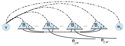
Figure 10: General presentation of an OLA $\varphi^{*}$ for $H=T\uplus C$, where $\varphi^{*}(v)$ while $v$ is not a leaf in tree $T$.

As apposed to layout $\varphi^{*}$ we present the following layout $\varphi^{\diamond}$.

$$\forall u\in V,\varphi^{\diamond}=\begin{cases}\varphi^{*}(u)+\sum_{j<i<k}\beta_{1,i}&\quad\text{if }u\in V(B_{1,j})\\ \mathcal{T}_{1}-\varphi^{*}(u)+1&\quad\text{if }u\in V(B_{1,j+1})\cup\dots\cup V(B_{1,k-1})\\ \mathcal{T}_{1}-\varphi^{*}(u)-\beta_{1,j}+1&\quad\text{if }u\in V(B_{1,1})\cup\dots\cup V(B_{1,j-1})\cup\{v\}\\ \varphi^{*}(u)&\quad\text{otherwise}\end{cases}$$

Where $\beta_{i,j}$ and $\mathcal{T}_{i}$ are respectively the number of vertices of branch $B_{i,j}$ and subtree $T_{i}$.

Informally speaking, layout $\varphi^{\diamond}$ is constructed by mirroring the labels of vertices of all the branches about $v$, except for the vertices of branch $B_{1,j}$. Figure 11 depicts the layout $\varphi^{\diamond}$.

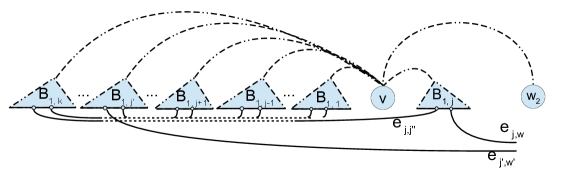
Figure 11: General presentation of an OLA $\varphi^{\diamond}$ based on $\varphi^{*}$, where the label of the vertices of branches are mirrored about vertex $v$ except those of branch $B_{1,j}$.

According to the construction of $\varphi^{\diamond}$ equation 43 holds. Note that the relative inter-orders of vertices of $B_{1,i}$ for $1\leq i<k$ (accordingly the size of expands of internal edges) stay unchanged in $\varphi^{\diamond}$.

(43) $$LA(\varphi^{*})-LA(\varphi^{\diamond})\geq$$

$$(\lambda(e_{j,w},\varphi^{*})-\lambda(e_{j,w},\varphi^{\diamond}))\ +$$

$$(\lambda(e_{j^{\prime},w^{\prime}},\varphi^{*})-\lambda(e_{j^{\prime},w^{\prime}},\varphi^{\diamond}))\ +$$

$$(\lambda(e_{j,j^{\prime\prime}},\varphi^{*})-\lambda(e_{j,j^{\prime\prime}},\varphi^{\diamond}))\ +$$

$$(\lambda(\{v,w_{2}\},\varphi^{*})-\lambda(\{v,w_{2}\},\varphi^{\diamond}))\ +$$

$$(\lambda(\{v,v_{j}\},\varphi^{*})-\lambda(\{v,v_{j}\},\varphi^{\diamond}))\ +$$

$$\sum_{j<i<k}(\lambda(\{v,v_{i}\},\varphi^{*})-\lambda(\{v,v_{i}\},\varphi^{\diamond}))$$

Each term of equation 43 refers to the change in the expands of those edges that their expand may change in the process of constructing $\varphi^{\diamond}$ from $\varphi^{*}$.

It’s not hard to verify that the following equations hold.

(44) $$(\lambda(e_{j,w},\varphi^{*})-\lambda(e_{j,w},\varphi^{\diamond}))=\sum_{j<i<k}\beta_{1,i}$$

(45) $$(\lambda(e_{j^{\prime},w^{\prime}},\varphi^{*})-\lambda(e_{j^{\prime},w^{\prime}},\varphi^{\diamond}))\geq-\sum_{1\leq i<k}\beta_{1,i}$$

(46) $$(\lambda(e_{j,j^{\prime\prime}},\varphi^{*})-\lambda(e_{j,j^{\prime\prime}},\varphi^{\diamond}))\geq-\sum_{1\leq i\leq j}\beta_{1,i}$$

(47) $$(\lambda(\{v,w_{2}\},\varphi^{*})-\lambda(\{v,w_{2}\},\varphi^{\diamond}))=\sum_{1\leq i<k,\ i\neq j}\beta_{1,i}$$

(48) $$(\lambda(\{v,v_{j}\},\varphi^{*})-\lambda(\{v,v_{j}\},\varphi^{\diamond}))=\sum_{1\leq i<j}\beta_{1,i}$$

(49) $$\sum_{j<i<k}(\lambda(\{v,v_{i}\},\varphi^{*})-\lambda(\{v,v_{i}\},\varphi^{\diamond}))=(k-j-1)\times\beta_{1,j}$$

Consequently equation 43 can be simplified as $LA(\varphi^{*})-LA(\varphi^{\diamond})\geq(k-j-3)\times\beta_{1,j}+\sum_{j<i<k}\beta_{1,i}$. The quantity $k-j-1$ is the number of branches labeled after $B_{1,j}$ and obviously $(k-j-1)\geq 1$. Hence for $(k-j-1)>1$ or $(k-j-1)=1\wedge\beta_{j+1}>\beta_{j}$, we have $LA(\varphi^{*})-LA(\varphi^{\diamond})>0$, which contradicts the optimality of $\varphi^{*}$. Now we analyze the case where $(k-j-1)=1\wedge\beta_{j+1}\leq\beta_{j}$.

Case 1: $B_{1,j}$ and $B_{1,j+1}$ are not connected.

Referring to the structure of Halin graphs, this case holds only if $j>1$. Informally speaking, there are some branches $B_{1,1},\ldots,B_{1,j-1}$ which based on $\varphi^{*}$ their vertices are labeled after $v$ and before $B_{1,j}$. With respect to this case we construct a new layout $\varphi^{\circledast}$ where the labels of vertices of $B_{1,1},\ldots,B_{1,j-1}$ are mirrored about $v$. Formally $\varphi^{\circledast}$ is constructed as:

$$\forall u\in V,\varphi^{\circledast}(u)=\begin{cases}\mathcal{B}+2-\varphi^{*}(u)&\quad\text{if }u\in V(B_{1,1})\cup\ldots\cup V(B_{1,j-1})\cup\{v\}\\ \varphi^{*}(u)&\quad\text{otherwise}\end{cases}$$

Where $\mathcal{B}=\sum_{1\leq i<j}\beta_{1,i}$ is the number of vertices in set $\{V(B_{1,1})\cup\ldots\cup V(B_{1,j-1})\}$.

Following the same approach as before we can show that $LA(\varphi^{*})-LA(\varphi^{\circledast})\geq\sum_{1\leq i<j}\beta_{1,i}>0$ . The details of arithmetic calculations are left to the reader.

Case 2: $B_{1,j}$ and $B_{1,j+1}$ are connected.

Hence $B_{1,j}$ and $B_{1,j+1}$ are the only branches connected to $v$. Figure 12(a) shows the layout $\varphi^{*}$ corresponding to this case. As schematically shown in figure 12(b), we present the the alternative layout $\varphi^{\circledast}$, formally defined as it follows.

$$\forall u\in V,\varphi^{\circledast}(u)=\begin{cases}\beta_{1,1}+2-\varphi^{*}(u)&\quad\text{if }u\in V(B_{1,1})\cup\{v\}\\ \varphi^{*}(u)&\quad\text{otherwise}\end{cases}$$

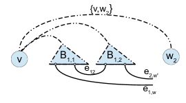
(a) OLA $\varphi^{*}$ where $\varphi^{*}(v)=1$ and $v$ is connected to exactly two branches $B_{1,1}$ and $B_{1,2}$.

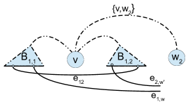
(b) The alternative non-overlapping layout $\varphi^{\circledast}$ based on $\varphi^{*}$, where the labels of vertices in $B_{1,1}$ are mirrored about $v$.

Figure 12: OLA $\varphi^{*}$ and the corresponding alternative layout $\varphi^{\circledast}$.

Equation 50 compares the value of linear arrangements $\varphi^{*}$ and $\varphi^{\circledast}$.

(50) $$LA(\varphi^{*})-LA(\varphi^{\circledast})=$$

$$(\lambda(\{v,w_{2}\},\varphi^{*})-\lambda(\{v,w_{2}\},\varphi^{\circledast}))\ +$$

$$(\lambda(\{v,v_{2}\},\varphi^{*})-\lambda(\{v,v_{2}\},\varphi^{\circledast}))\ +$$

$$(\lambda(e_{1,2},\varphi^{*})-\lambda(e_{1,2},\varphi^{\circledast}))\ +$$

$$(\lambda(e_{1,w},\varphi^{*})-\lambda(e_{1,w},\varphi^{\circledast}))$$

Remember that $v_{1}$ and $v_{2}$ are the two vertices where $B_{1,1}$ and $B_{1,2}$ are anchored at.

Based on the construction of $\varphi^{\circledast}$ from $\varphi^{*}$ we have:

(51) $$\lambda(\{v,w_{2}\},\varphi^{*})-\lambda(\{v,w_{2}\},\varphi^{\circledast})=\beta_{1,1}$$

(52) $$\lambda(\{v,v_{2}\},\varphi^{*})-\lambda(\{v,v_{2}\},\varphi^{\circledast})=\beta_{1,1}$$

(53) $$\lambda(e_{1,2},\varphi^{*})-\lambda(e_{1,2},\varphi^{\circledast})\geq-\beta_{1,1}$$

(54) $$\lambda(e_{1,w},\varphi^{*})-\lambda(e_{1,w},\varphi^{\circledast})\geq-\beta_{1,1}$$

Finally putting equations 50 to 54 together we conclude that $LA(\varphi^{*})-LA(\varphi^{\circledast})\geq 0$. But the equalities in equations 53 and 54 hold at the same time (and consequently $LA(\varphi^{*})-LA(\varphi^{\circledast})=0$), only if the two edges $e_{1,2}$ and $e_{1,w}$ coincide at the left most vertex of $B_{1,1}$. This situation in a Halin graph can only happen when branch $B_{1,1}$ has exactly one vertex. For that reason we conclude that in an OLA for a Halin graph $H=T\uplus C$, a non-leaf vertex $v$ can be a extreme vertex, only if $v$ has exactly two leaves of $T$ as it’s children.

References

- [1] FRK Chung. On optimal linear arrangements of trees. Computers & mathematics with applications, 10(1):43–60, 1984.
- [2] Johanne Cohen, Fedor Fomin, Pinar Heggernes, Dieter Kratsch, and Gregory Kucherov. Optimal linear arrangement of interval graphs. In Mathematical Foundations of Computer Science 2006, pages 267–279. Springer, 2006.
- [3] T Easton, S Horton, and RG Parker. A solvable case of the optimal linear arrangement problem on halin graphs. Congressus Numerantium, pages 3–18, 1996.
- [4] Shimon Even and Yossi Shiloach. Np-completeness of several arrangement problems. Dept. Computer Science, Technion, Haifa, Israel, Tech. Rep, 43, 1975.
- [5] M. R. Garey, David S. Johnson, and Larry J. Stockmeyer. Some simplified np-complete graph problems. Theor. Comput. Sci., 1(3):237–267, 1976.
- [6] MK Goldberg and IA Klipker. An algorithm for minimal numeration of tree vertices. Sakharth. SSR Mecn. Akad. Moambe, 81(3):553–556, 1976.
- [7] Steven B Horton, T Easton, and R Gary Parker. The linear arrangement problem on recursively constructed graphs. Networks, 42(3):165–168, 2003.
- [8] David S Johnson. The np-completeness column: an ongoing guide. Journal of Algorithms, 6(3):434–451, 1985.
- [9] Jordi Petit. Addenda to the survey of layout problems. Bulletin of EATCS, 3(105), 2013.
- [10] Habib Rostami and Jafar Habibi. Minimum linear arrangement of chord graphs. Applied Mathematics and Computation, 203(1):358–367, 2008.
- [11] Yossi Shiloach. A minimum linear arrangement algorithm for undirected trees. SIAM Journal on Computing, 8(1):15–32, 1979.