Monte Carlo Simulations of the site-diluted 3$d$ XY model with superexchange interaction: application to Fe[Se₂CN(C₂H₅)₂]₂Cl – Zn[S₂CN(C₂H₅)₂]₂ diluted magnets

Abstract

A simple site-diluted classical XY model is proposed to study the magnetic properties of the ferromagnetic polycrystalline Fe[Se₂CN(C₂H₅)₂]₂Cl diluted with diamagnetic Zn[S₂CN(C₂H₅)₂]₂. An extra superexchange interaction is assumed between next-nearest-neighbors on a simple cubic lattice, which are induced by a diluted ion. The critical properties are obtained by Monte Carlo simulations using a hybrid algorithm, single histograms procedures and finite-size scaling techniques. Quite good fits to the experimental results of the ordering temperature are obtained, namely its much less rapidly decreasing with dilution than predicted by the standard diluted 3$d$ XY model, and the change in curvature around $86\%$ of the magnetic Fe[Se₂CN(C₂H₅)₂]₂Cl compound.

The critical behavior of disordered magnetic systems has been the subject of a great amount of investigations during the last few decades both theoretically and experimentally(see, for instance, stinch ; liu and references therein). On the theoretical point of view, one of the extensively studied models is the site diluted XY model. The XY model was originally introduced by Matsubara and Matsuda Matsubara to describe the behavior of liquid helium santosfilho2 , but has also been quite suitable to describe the critical behavior of some anisotropic insulating antiferromagnets Betts ; Betts2 . The three-dimensional (3$d$) version of the classical XY model with site dilution also showed a good agreement with some experimental results of some physical realizations, such as the antiferromagnets Co_1-xZn_x(C₅H₅NO)₆(ClO₄)₂ Algra and [Co_pZn$1_{p}$(C₅H₅NO)](NO₃)₂ Burriel . Recently, however, DeFotis et al. DeFotis presented the phase diagram for the pentacoordinate iron(III) molecular ferromagnet, in which the simple site diluted XY model predictions are in complete disagreement with the experimental data.

The pentacoordinate iron(III) molecular ferromagnet Fe[Se₂CN(C₂H₅)₂]₂Cl is, to date, the only known material to exhibit three-dimensional XY ferromagnetic behavior DeFotis2 . Exchange interactions occur via intermolecular Se$-$Se contacts, the selenium atoms being covalently bonded to the iron, leading to a ferromagnetic ordering near $3.4$ K . The magnetic lattice is a simple cubic one and this random compound, when diluted with non-magnetic Zn[S₂CN(C₂H₅)₂]₂, presents an initial critical temperature slope $s=\left[(dTc/dp)/Tc\right]_{p=1}=0.24(2)$ DeFotis , where $p$ is the concentration of the magnetic material Fe[Se₂CN(C₂H₅)₂]₂Cl (the concentration of the non-magnetic material Zn[S₂CN(C₂H₅)₂]₂ is $q=1-p$). This slope is well below the theoretical predictions for the $3d$ simple cubic XY model with site dilution, whose value is $s=1.0965(39)$ santosfilho , and even below the slope for the Ising and Heisenberg models. In addition, there is also an inflection point in the critical temperature as a function of the concentration $p$, which can not be accounted for by these simple diluted models either. So, these striking behavior seem not to be a model question, but some other microscopic feature instead.

In ref. DeFotis the authors have indeed commented on a possible superexchange pathway (although they claimed it seems not be so effective) between Fe atoms which might be responsible for the weak decline in the critical temperature with dilution. We will here pursue exactly in this direction and show that a superexchange interaction can in fact account for this small decline of the transition temperature with magnetic site concentration, and even for the inflection point, with a good agreement with the experimental data.

So, in this work, without taking into account the complex lattice structure of the pentacoordinate iron(III) molecular ferromagnet, we propose an extended version of the simple site-diluted XY model, defined on a simple cubic lattice, in the same lines as the works on Fe-Al pla1 ; pla2 as well as on Fe-Al-Mn systems Alcazar . In order to study the phase diagram of this disordered system, we further assume herein that the dopant, or the non-magnetic ion, can induce a superexchange like ferromagnetic interaction between its nearest-neighbor spins.

Thus, the system under investigation is given by a quenched site-diluted XY model Hamiltonian that can be written as

$$\begin{split}\mathcal{H}=&-J_{1}\sum_{\langle i,j\rangle}\epsilon_{i}\epsilon_{j}[S_{i}^{x}S_{j}^{x}+S_{i}^{y}S_{j}^{y}]\\ &-J_{2}\sum_{\langle\langle i,j\rangle\rangle}\epsilon_{i}\epsilon_{j}[S_{i}^{x}S_{j}^{x}+S_{i}^{y}S_{j}^{y}]\leavevmode\nobreak\ ,\end{split}$$ (1)

where the first sum is over nearest-neighbors (NN) $\langle i,j\rangle$ spins, the second sum over next-nearest-neighbors (NNN) $\langle\langle i,j\rangle\rangle$ spins, $\vec{S_{i}}$ represents a three-dimensional classical spin $\vec{S_{i}}=(S^{x}_{i},S^{y}_{i},S^{z}_{i})$, where $S_{i}^{\alpha}$ are the $\alpha=x,\leavevmode\nobreak\ y,$ and $z$ cartesian components of $\vec{S_{i}}$ with $S_{i}^{2}=(S^{x}_{i})^{2}+(S^{y}_{i})^{2}+(S^{z}_{i})^{2}=1$. $J_{1}>0$ is the NN and $J_{2}>0$ is the NNN ferromagnetic interactions, respectively. While the first sum in Eq. (1) runs over all nearest-neighbor pairs, the second sum runs only over the next-nearest-neighbor pairs having a dopant as a common nearest-neighbor, i.e., for situations in the lattice where a non-magnetic site $k$ has the corresponding sites $i$ and $j$ as NN. In this sense, in a simple cubic lattice, which is the case for the pentacoordinate iron(III) molecular ferromagnet, depending on its concentration, a non-magnetic molecule can break up to six interactions $J_{1}$ and, on the other hand, can generate up to twelve interactions $J_{2}$.

In Eq.(1), $\epsilon_{i}$ are quenched, uncorrelated random variables, representing the existence of two kinds of particles in the system, namely the magnetic ones with $\epsilon_{i}=1$, and non-magnetic ones with $\epsilon_{i}=0$. The variable $\epsilon_{i}$ is chosen according to the probability distribution

$$P(\epsilon_{i})=p\delta(\epsilon_{i}-1)+(1-p)\delta(\epsilon_{i}),$$ (2)

where $p$ is the concentration of magnetic sites, such that $p=1$ corresponds to the pure case.

The above Hamiltonian has been studied through Monte Carlo simulations. First, we prepare a diluted lattice where a given configuration of diluted sites $\{\epsilon\}$ refers to a single sample. For every thermodynamic observable $Q$, we first calculate the thermal average $\langle Q_{\{\epsilon\}}\rangle$ for a given sample $\{\epsilon\}$ and the results for different samples are later averaged as $\left[{\left\langle{Q_{\left\{\epsilon\right\}}}\right\rangle}\right]_{{\text{av}}}$. In order to get the critical properties of the present model, for each sample of a given site-disorder configuration $p$, we used a hybrid Monte Carlo algorithm consisting of one single spin Metropolis algorithm, and one overrelaxation updates of the spins at constant configurational energy creutz ; pawig . This hybrid Monte Carlo method prb60 has been implemented, and has been shown to reduce correlations between successive configurations in the simulation (santosfilho, ). Close to the transition temperature we have also resorted to single histogram techniques to get the corresponding thermodynamic quantities. We have first computed the in-plane-magnetization, magnetic susceptibility, and the Binder cumulant given, respectively, by

$$m_{xy}=\frac{1}{L^{2}}\sum_{i=1}^{L^{3}}[(S_{i}^{x})^{2} + (S_{i}^{y})^{2}],$$ (3)

$$\chi=L^{2}\frac{\langle m_{xy}^{2}\rangle-\langle m_{xy}\rangle^{2}}{T} \leavevmode\nobreak\ \leavevmode\nobreak\ u_{4}=1-\frac{\langle m_{x}^{4}\rangle}{3\langle m_{x}^{2}\rangle^{2}},$$ , (4)

where $L$ is the linear size of the cubic lattice studied, $T$ is the temperature given in units of $J/k_{B}$, $k_{B}$ being the Boltzmann constant, and for the cumulant we have $m_{\alpha}^{m}=\left({\frac{1}{L^{3}}}\sum_{i=1}^{L^{3}}{S_{i}^{\alpha}}\right)^{m}$, with $\alpha=x,y,$ or $z$. We have also considered $J_{1}=1$, in such a way that $J_{2}$ is measured in units of $J_{1}$. Although the natural, or standard, choice of the Binder cumulant in the context of an XY type transition would include both the $x$- and $y$-components of the magnetization massimo , it has been previously shown the $x$ component to be the most suitable one for computing $u_{4}$ and getting the criticality of the model prb60 .

In addition, to reach the final results, for each dilution, temperature, and lattice size, the MC estimates $\langle Q_{\{\epsilon\}}\rangle$ of thermodynamic quantities, for a given random distribution $\{\epsilon\}$ of diluted sites were averaged over different disorder realizations as

$$\left[{\left\langle{Q_{\left\{\epsilon\right\}}}\right\rangle}\right]_{{\text{av}}}=\frac{1}{{\#\left\{\epsilon\right\}}}\sum\limits_{\left\{\epsilon\right\}}{\left\langle{Q_{\left\{\epsilon\right\}}}\right\rangle},$$ (5)

with $\#\{\epsilon\}$ the number of total realizations considered.

Now, regarding the simulational numbers, for every sample the runs comprised $10^{3}$ MCS per spin for equilibration and the measurements were made over $5\times 10^{4}$ MCS. The lattice sizes raged from $L=10$, $20$, $30$, $40$, the values being chosen so that $p\times L^{3}$ gives an integer number. We have used in the present paper $100$ samples for all settings. As discussed in ref. santosfilho , such simulations could give a good account of the model with only NN interactions, even concerning the critical exponents. We believe the same happens for this more general model, mainly for the critical temperature, which is our main purpose for the experimental data we are comparing to.

The critical temperature $T_{c}$ was obtained from the peak of susceptibility and cumulant crossing for different values of $L$. We have used the correlation length critical exponents of the XY universality class since it is independent of the value of the dilution santosfilho . The quality of the results are the same as those obtained for the pure model and extensively discussed in ref. santosfilho . For this reason, we will only present herein the corresponding results for the critical temperature.

Fig. 1 exhibits, for several values of the NNN interaction $J_{2}$, the reduced transition temperature $T_{c}(p)/T_{c}(1)$ as a function of $p$, where $T_{c}(p)$ is the critical temperature for the concentration $p$ and $T_{c}(1)$ is the transition temperature of the pure system. In this case, as just a matter of comparison, we have considered ordinary next-nearest-neighbor interactions $J_{2}$, in the sense that no superexchange character has been implemented. It means that second-neighbors interact, independently of their neighborhood. One can clearly see that, as the next-nearest-neighbor interactions increase, the slope close to $p=1$ decreases. Nevertheless, no value of $J_{2}$ can give a satisfactory behavior of the transition temperature in the wider range of concentrations analysed experimentally. This means that the dilution alone is not responsible for the experimental phase diagram.

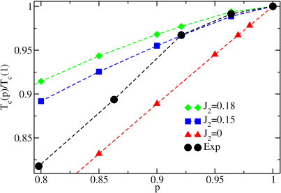
Figure 1: (Color online) Reduced critical temperature $T_{c}(p)/T_{c}(1)$ as a function of the mangnetic sites concentration $p$, for several values of the next-nearest-neighbor interaction $J_{2}$ ($J_{1}=1$). The experimental results, represented by the circles, were taken from Ref.DeFotis . The other symbols are simulation results. The dasheds lines are just guide to the eyes. The simulational errors are smaller than the symbol sizes.

The situation is indeed completely different when we further assume that the NNN interaction $J_{2}$ is induced by a diluted site, or a dopant, in a kind of superexchange interaction. Recall that, in this case, only impurities whose nearest neighbors are magnetic sites enable the arising of a superexchange interaction between NNN magnetic sites. In addition, another effect should be included in the simulations. In Fig. 2(a) one has a square lattice view of a non-magnetic dopant where four NNN interactions are induced. However, when one has a cluster of two dopants, as in Fig. 2(b), they tend to get closer, since the unit cell of the selenium material is 11.3% larger due to the greater size of Se versus S DeFotis . So, the distance from the dopant tends to increase in this case, and one expects a smaller superexchange interaction $J_{2}^{\prime}$. The same will happen for a $J_{2}^{\prime\prime}$ when three dopants are closer, and so on. When we consider $J_{2}=J_{2}^{\prime}=J_{2}^{\prime\prime}=...$, we recover the ordinary NNN interaction model results shown in Fig. 1. Nevertheless, by assuming that only $J_{2}$ is sufficiently high (i.e. $J_{2}^{\prime}=J_{2}^{\prime\prime}=...=0$) we arrive at a global phase diagram depicted in Fig. 3. In this figure we have the results for $J_{2}=0.18$ and $J_{2}=0$ as well. One can notice now a good agreement with the experimental results. The theoretical critical line of the $J_{2}=0$ model goes to the limit of the percolation threshold of the simple cubic lattice (we have not done simulations for $p<0.4$, because in this case the transition temperature is very small). Moreover, for larger non-magnetic concentrations, the results from the model considering next-nearest-neighbor interactions approach those of the pure model. This is understandable, since the higher the dilution, the more difficult it becomes to create new superexchange interactions, and the system ends up with only NN interactions (a fact that does not happen in the model with ordinary NNN couplings).

(a)

(b)

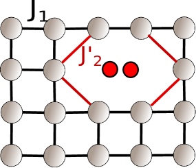
Figure 2: (Color online) A square lattice sketch of the induced superexchange interaction $J_{2}$ by the dopant (isolated circles). In (a), one dopant generates the NNN interaction $J_{2}$. In (b), a cluster of two dopants (on an exaggerated scale). They are now farther from the magnetic ions and one has a NNN $J_{2}^{\prime}<J_{2}$.

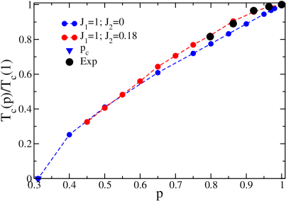
Figure 3: (Color online) The same as Fig. 1, for $J_{2}=0$ and $J_{2}=0.18$, assuming that the superexchange interaction $J_{2}$ is induced by the presence of a diluted site. $p_{c}$ is the percolation threshold for the simple cubic lattice.

It is also interesting to look at the phase diagram closer to the pure model, as is shown in Fig. 4, where the discrepancy from the simple site diluted model and the one considering superexchange next-nearest-neighbor interactions is clearer still. In addition to the quite good fits to the experimental data, one can also note, from the inset in Fig. 4, that the present model also exhibits an inflection point around $p=0.80(5)$, close to $p=0.86$ that is experimentally observed.

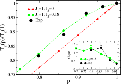
Figure 4: (Color online) A closer view of the phase diagram from Fig. 3 in the region near the pure system for $J_{2}=0$ and $J_{2}=0.18$. The inset shows the estimate of the corresponding slopes as a function of $p$. The arrows indicate the inflection point. Regarding the simulations, the errors are smaller than the symbols sizes.

In summary, we have proposed a simple diluted XY model on a simple cubic lattice where superexchange interactions are induced between NNN via dilution sites. Not only the slow slope of the critical temperature as a function of the concentration agrees well with the experimental data, but also an inflection point of the critical curve is present, and quite close to the corresponding experimental concentration. Of course, this is only a theoretical assumption still needing a more experimental evidence.

A little more words are, however, worthwhile in commenting the present simulations. First, it is well known that MC simulations are not suitable in adjusting theoretical parameters to experimental data, mainly due to computational costs. In the present case things are better in the sense that we have just one parameter. As one knows the critical temperature for the pure XY three-dimensional model with reasonable accuracy, this serves to estimate $J_{1}$. But, renormalizating the critical temperature data by its value for the pure model, we can get rid of $J_{1}$ and just fit in fact the ratio $J_{2}/J_{1}$. So, as we can further consider $J_{1}=1$ in our equations, all the simulations have to be done for different values of the next-nearest-neighbor coupling ratio. This makes the fitting problem an easier one.

As a second remark, we recall that we have used FSS to get $T_{c}(p)$, so the corresponding values of the critical temperature are indeed very accurate. This means that any problems with the comparison to the experimental data, if any, would be related to the quantum nature of the spin state, since we have considered a classical spin model. However, as Fe ion can have a spin-$3/2$, the use of a classical model can, in some sense, be suitable for the present case.

As a final comment, from the critical temperature of the pure model $k_{B}T_{c}/J_{1}=1.5518$ santosfilho one can estimate the nearest-neighbor interaction $J_{1}=0.189$ meV, which should be compared to $12.8$ meV obtained for the Fe-Mn-Al alloys pla1 ; pla2 ; Alcazar (or to $10-50$ meV as is usual for ferromagnetic systems). These two orders of magnitude smaller can be understood since for the present system the ordering temperature is very low, near $3.4$ K, instead of about $1000$ K, as is the case of the Fe based alloys. On the other hand, the ratio $J_{2}/J_{1}=0.18$ is within of what is expected for a second-neighbor interaction. Of course, more theoretical and experimental studies on these systems would be very welcome.

- (1) R. Stinchcombe, Phase Transitions and Critical Phenomena, edited by C. Domb and J. L. Lebowitz (Academic, London, 1983), Vol. 7.
- (2) Y. Liu, D. Shindō, and D. J. Sellmyer, Handbook of advanced magnetic materials, edited by Yi Liu , D. J. Sellmyer and D. Shindo, (Springer, New York, 2005), Vol. 3.
- (3) T Matsubara and H Matsuda, Progress of Theoretical Physics,16 569-582 (1956)
- (4) J. B. Santos-Filho, J. A. Plascak, and D. P. Landau. Physica A: Statistical Mechanics and its Applications 389(15) 2934-2938(2010)
- (5) D. D. Betts and M. H. Lee, Phys. Rev. Lett. 2026, 1507 (1968)
- (6) D. D. Betts, Physica B+ C 86 556 (1977)
- (7) H. A. Algra,L. J. De Jongh, W. J. Huiskamp, and J. Reedijk. Physica B+ C,86, 737-739. (1977)
- (8) R. Burriel, A. Lambrecht, R. L. Carlin and L. J. de Jongh. Phys. Rev. B, 36(16), 8461.(1987)
- (9) G. C. DeFotis, R. A. Huddleston, B. R. Rothermel, J. H. Boyle, E. S. Vos, Y. Matsuyama, A. T. Hopkinson, T. M. Owens, and W. M. May, J. Phys.: Cond. Matt. 20, 135222 (2008).
- (10) G. C. DeFotis,B. K. Failon, F. V. Wells,H. H. Wickman,Physical Review B 29(7), 3795-3809 (1984).
- (11) J. B. Santos-Filho, and J. A. Plascak. Computer Physics Communications, 182(5), 1130-1133 (2011).
- (12) J. A. Plascak, L. E. Zamora, and G. A. Pérez Alcázar, Phys. Rev. B 61, 3188 (2000).
- (13) D. A. Dias, J. Ricardo de Sousa, and J. A. Plascak, Phys. Lett. A 373, 3513 (2009).
- (14) G.A. Perez Alcazar, J.A. Plascak, and E. Galvão Silva, Phys. Rev. B 38, 2816 (1988).
- (15) A. B. Harris, J. Phys. C 7, 1671 (1974); A. B. Harris and T. C. Lubensky, Phys. Rev. Lett. 33, 1540 (1974).
- (16) M. Creutz, Phys. Rev. D 36, 515 (1987).
- (17) S. G. Pawig and K. Pinn, Int. J. Mod. Phys. C 9, 727 (1998).
- (18) M. Campostrini, M. Hasenbusch, A. Pelissetto, and E. Vicari, Phys. Rev. B 74, 144506 (2006).
- (19) M. Krech and D. P. Landau, Phys. Rev. B 60, 3375 (1999).