Discriminative Prototype Set Learning for Nearest Neighbor Classification

Abstract

The nearest neighbor rule is a classic yet essential classification model, particularly in problems where the supervising information is given by pairwise dissimilarities and the embedding function are not easily obtained. Prototype selection provides means of generalization and improving efficiency of the nearest neighbor model, but many existing methods assume and rely on the analyses of the input vector space. In this paper, we explore a dissimilarity-based, parametrized model of the nearest neighbor rule. In the proposed model, the selection of the nearest prototypes is influenced by the parameters of the respective prototypes. It provides a formulation for minimizing the violation of the extended nearest neighbor rule over the training set in a tractable form to exploit numerical techniques. We show that the minimization problem reduces to a large-margin principle learning and demonstrate its advantage by empirical comparisons with other prototype selection methods.

keywords: Nearest neighbor rule, Prototype selection, Soft maximum, Large-margin principle

1 Introduction

The nearest neighbor rule is one of the most widely used models for classification [22, 29] and essential in domains where the objects are characterized by pairwise dissimilarities, e.g, protein structures and genome sequences in biochemistry and population or groups of people in economics and psychology. The supervising information for such objects is often provided as a matrix of mutual dissimilarities, which the nearest neighbor rule can directly exploit.

Many classification models require training samples characterized by a set of features and represented as vectors. It is thus necessary to find an embedding of objects onto a Euclidean space in order to exploit such models for dissimilarity data. Such techniques have been studied in the context of multi-dimensional scaling [26] and have been incorporated with discriminative learning principles such as structural risk minimization [16]. Another example of this approach is the approximate nearest neighbor search (ANNS) [2, 23], which employs locality sensitive hashing (LSH) for a probabilistic embedding of objects onto a low-dimensional space. These techniques, however, are respectively subject to some assumptions regarding, e.g., the properties of the embedded space or the functions used to compute dissimilarities.

The nearest neighbor classification model, on the other hand, is quite unconstrained, but the issues of memory and computational efficiency for finding nearest neighbors are critical in practice [7]. Prototype selection methods provide the means to reduce the time and space complexity for nearest neighbor computation and to generalize the nearest neighbor rule, by selecting a set of prototypes from the full training data for the prediction on the test data. Although there has been a substantial amount of literature on prototype selection published in the topic of data mining, many such techniques exploit the analysis of the feature space, e.g., removing prototypes far from the decision boundary of two classes to reduce redundancy or conversely, removing those near the boundary for generalization [27]. In addition, these models require the wrapper technique and cross validation to empirically tune parameters [22] which are computationally expensive, due to their intractable formulations.

In this paper, we revisit the prototype selection problem to explore a parametric approach based on a discriminative learning principle. The key intuition of the proposed approach is two-fold. First, we define a parametric extension of the nearest neighbor rule, in which the choice of the nearest neighbor is adjusted by a numerical parameter assigned to each prototype. The parameter values are also used to infer whether the instances are relevant for prediction. Secondly, we introduce a differentiable approximation of the condition that the nearest neighbor rule predicts the class of a training instance correctly, and subsequently derive a constrained optimization problem for minimizing the violation of the condition with regards to the numerical parameters of the prototypes. We further show that this problem reduces to a large-margin principle learning using a sparse representation of the relations between the neighboring instances.

In summary, the contribution of this work is a prototype selection method, which (a) can exploit complex distance or dissimilarity functions and do not rely on the presence and the analysis of the vector space and (b) enables an optimization algorithm for learning the parameters to extend the nearest neighbor rule. The rest of this paper is organized as follows. Section 2 discusses the related work. Section 3 describes the proposed method Section 5 shows the results of our empirical study. Section 6 presents our conclusion.

2 Related Work

The weaknesses of the nearest neighbor classifier in terms of large time and memory requirements respectively for computing and storing the similarities is well-known. One way to address this issue is to reduce the number of prototypes at the pre-processing phase. This problem has been referred to as prototype selection [13], data reduction [28], instance selection [14, 15, 19], and template reduction [12, 24]. The goal of the problem is to find a compact subset of the prototypes which maintains or possibly improve the generalization error of the nearest neighbor classification while decreasing the computational burden.

The above methods typically employ operations such as editing, which eliminates or relocates noisy prototypes that cause misclassifications near the borders of different classes [7, 28] for the effects of smoothing and generalizing the decision boundaries. Condensation is another common operation, which discards prototypes far from the class borders in order to reduce the redundancy of the prototype set without affecting the decision boundary [3].

The above methods are generally implemented with the wrapper or the filtering techniques [22]. The wrapper technique evaluates and selects different sets of prototypes based on the performance of the nearest neighbor classifier. The filtering technique selects prototypes based on their individual scores, which are less expensive to compute than the performance measure.

3 Proposed Method

3.1 Preliminaries

Let $\mathcal{X}=\{{x}_{i}\}_{i=1}^{n}$ denote the set of labeled instances and $\mathcal{Y}=\{y_{i}\}_{i=1}^{n}$ their class values. Instances are not necessarily represented as vectors, as the nearest neighbor prediction requires only similarities/dissimilarities from the prototypes to a new instance. The nearest neighbor classifier, $h$, returns the class prediction on a test sample ${t}$ as follows.

(3.1) $$\small h({t})=y_{i}:\mathop{\arg\min}\limits_{i\in\{1,\ldots,n\}}{d}({t},{x}_{i})$$

where ${d}(\cdot,\cdot)$ denotes the dissimilarity function. A prototype selection algorithm selects a subset $\mathcal{Z}\subseteq\mathcal{X}$ with which the nearest neighbor classifier yields smaller generalization error and run-time.

In order to evaluate a candidate prototype set in the training phase, one must avoid trivial cases where the target instance being classified is also one of the prototypes set, as the prototypes and the training instances originally come from the same set of instances, $\mathcal{X}$. In the following sections, we employ a setup similar to the leave-one-out cross validation, such that the target instance is always removed from the prototype set. That is, the prototypes for predicting the class of $x_{i}$ will be a subset of the remainder of the labeled instances, denote by $\mathcal{Z}_{i}=\mathcal{X}\setminus\{x_{i}\}$. For distinction, we refer to an instance as a prototype only when it is used as one of the reference objects for the nearest neighbor rule, in this paper. In turn, we refer to an instance as a training instance only when it is the subject of prediction.

3.2 Soft-Maximum Function

The soft maximum [6] is an approximation of the function $\max(\cdot,\cdot)$ as $\log\left(\exp(\cdot)+\exp(\cdot)\right)$. The approximation is convex and differentiable, which are desirable for numerical optimization.

A natural extension of the soft maximum for $m$ variables $x_{1},\ldots,x_{m}$ is given by

(3.2) $$\small\mathcal{M}(x_{1},\ldots,x_{m})=\log\sum_{i=1}^{m}\exp({x_{i}})$$

The base of the exponential, $\beta$, is larger than 1 and adjusted for the scale of the input values.

3.3 Adjusted Nearest Neighbor Rule

This section introduces an extension of the nearest neighbor rule to parametrize the model and the prototype selection problem.

Let $x$ denote a target instance and $\mathcal{Z}$ denote the set of prototypes. We denote by $R(x,x_{j};\mathcal{Z})$ the rank of $d(x,x_{j})$ in the set $\left\{d(x,x_{j})\right\}_{x_{j}\in\mathcal{Z}}$. The rank takes an integer value from $\{1,\ldots,\#\mathcal{Z}\}$ and a smaller integer is a higher rank. The nearest neighbor rule for a target instance $x$ is given as follows.

• Compute distances $\{d(x,x_{j})\}_{x_{j}\in\mathcal{Z}}$

• Assign rank $R(x,x_{j};\mathcal{Z})$ to all $x_{j}\in\mathcal{Z}$ based on their distances to $x$

• Return the class of the highest-ranked $x_{j}$

We introduce a non-negative parameter $\alpha(x_{j})$ for each prototype to compute the adjusted rank $R^{\prime}$.

(3.3) $$\small R^{\prime}(x,x_{j};\mathcal{Z})=R(x,x_{j};\mathcal{Z})+\alpha(x_{j})$$

The adjusted nearest neighbor rule generalizes the nearest neighbor rule and produces identical predictions when $\alpha(x_{1})=\ldots=\alpha(x_{n})$.

Based on the adjusted ranks, the nearest prototype can be passed over for another prototype. We thus refer to $\alpha(x_{j})$ as the degradation parameter of the prototype $x_{j}$. For brevity, we will use $\alpha_{j}$ as $\alpha(x_{j})$ when it is clear from context. One may correct individual misclassifications by assigning larger degradations to the related prototypes. That is, if $x_{j}$ and $x_{k}$ are respectively the highest and the second highest-ranked prototypes for a training case $(x,y)$ where $y_{j}\neq{y}$ and $y_{k}={y}$, the misclassification may be avoided by assigning a relatively larger degradation to $\alpha_{j}$ than $\alpha_{k}$.

The aim of this extension is to enable the training of the degradation parameters to improve the classification performance over all hold-out cases. Based on their values, we can identify which prototypes are more relevant for prediction and reduce the prototype set accordingly. The motivation for focusing on ranks rather than distances is to avoid the issue of scaling. The latter may vary substantially in scale depending on the function, thus may require ad-hoc adjustments.

3.4 Approximate Nearest Neighbor Rule

Let $(x_{i},y_{i})$ denote a pair of a hold-out instance and its class label. We denote by $\mathcal{P}$ the subset of prototypes $\mathcal{Z}_{i}$ with the same label as $y_{i}$ and $\mathcal{Q}$ that of labels other than $y_{i}$. The condition that the nearest neighbor rule correctly predicts $y_{i}$ is that its nearest neighbor is an element of $\mathcal{P}$. That is,

(3.4) $$\small\max\left(\left\{-{d}(x_{i},p)\right\}_{p\in\mathcal{P}}\right)>\max\left(\left\{-{d}(x_{i},q)\right\}_{q\in\mathcal{Q}}\right)$$

Note that the trivial prediction does not occur because $x_{i}$ is not an element of $\mathcal{P}$.

In an ideal prototype set, the condition (3.4) is satisfied over all training cases for all ${x_{i}}\in\mathcal{X}$. There may not exist such an ideal set in general, and thus a practical goal for selecting the prototypes is to reduce the cases where the conditions are violated, as much as possible.

The formulation of such a principal is non-trivial due to the $\max$ function in (3.4). Alternatively, we rewrite (3.4) substituting the soft maximum $\mathcal{M}$ and the ranks of $d(x_{i},q)$ and $d(x_{i},p)$ for $\max$ and the distance values, respectively.

(3.5) $$\mathcal{M}\left(\{-R(x_{i},p;\mathcal{Z}_{i})\}_{p\in\mathcal{P}}\right)\geq$$

$$\mathcal{M}\left(\{-R(x_{i},q;\mathcal{Z}_{i})\}_{q\in\mathcal{Q}}\right)+1,\forall{x_{i}}\in\mathcal{X}$$

In essence, (3.5) describes the same condition as (3.4) with regards to the ranks of the prototypes of the same and different classes in the hold-out case. The constant 1 is added to the RHS given that $R$ is the rank taking an integer value.

Substituting (3.2) to (3.5), we have

$$\log\left(\sum_{p\in\mathcal{P}}\exp\left({-R\left(x_{i},p;\mathcal{Z}_{i}\right)}\right)\right)$$

$$\geq \log\left(\sum_{q\in\mathcal{Q}}\exp\left(-R\left(x_{i},q;\mathcal{Z}_{i}\right)\right)\right)+1$$

Taking the exponential on both sides, we obtain

(3.7) $$\sum_{p\in\mathcal{P}}\exp\left(-R(x_{i},p;\mathcal{Z}_{i})\right)$$

$$-\sum_{q\in\mathcal{Q}}\exp\left({-R\left(x_{i},q;\mathcal{Z}_{i}\right)}\right)\geq\rho(x_{i})$$

where $\rho(x_{i})$ is

(3.8) $$\small\rho(x_{i})=(\beta-1)\sum_{q\in\mathcal{Q}}\exp\left({-R\left(x_{i},q;\mathcal{Z}_{i}\right)}\right)$$

Rewriting the LHS of (3.4) given $\mathcal{P}\cup\mathcal{Q}=\mathcal{Z}_{i}$,

(3.9) $$\small\sum_{x_{j}\in\mathcal{Z}_{i}}\delta(y_{i},y_{j})\exp\left({-R\left(x_{i},x_{j};\mathcal{Z}_{i}\right)}\right)\geq\rho(x_{i})$$

where $\displaystyle\delta(y_{i},y_{j})=\left\{\begin{matrix}1&\text{if\,}y_{i}=y_{j}\\ -1&\text{otherwise}\end{matrix}\right.$

Considering (3.9) a constraint of nearest neighbor rule for each $x_{i}$, we introduce a slack variable $\xi_{i}$ to represent the violation.

(3.10) $$\sum_{x_{j}\in\mathcal{Z}_{i}}\delta(y_{i},y_{j})\exp\left({-R\left(x_{i},x_{j};\mathcal{Z}_{i}\right)}\right)$$

$$\phantom{===}\geq\rho(x_{i})-\xi_{i}$$

Each $\xi_{i}$ takes a non-negative value, and the violation of the nearest neighbor rule over the training set is given as $\sum_{x_{i}\in\mathcal{X}}\xi_{i}$.

3.5 Problem Formulation

Combining the rank degradation parameter and the soft-max approximation, we formulate a constrained optimization problem for the parametrized nearest neighbor classification model.

Rewriting (3.10) with the adjusted rank,

(3.11) $$\sum_{x_{j}\in\mathcal{Z}_{i}}\delta(y_{i},y_{j})\exp\left({-R\left(x_{i},x_{j};\mathcal{Z}_{i}\right)}-\alpha(x_{j})\right)$$

$$\geq\rho^{\prime}(x_{i})-\xi_{i}$$

where $\rho^{\prime}(x_{i})$ is the residual term that corresponds to $\rho(x_{i})$ in (3.10), i.e.,

$$\rho^{\prime}(x_{i}) = (\beta-1)\sum_{q\in\mathcal{Q}}\exp\left({-R^{\prime}\left(x_{i},q;\mathcal{Z}_{i}\right)}\right)$$

$$= (\beta-1)\sum_{q\in\mathcal{Q}}\exp\left(-R\left(x_{i},q;\mathcal{Z}_{i}\right)-\alpha(q)\right)$$

(3.11) is not a desirable form for a constrained optimization problem because the parameter being trained appears on both sides. That is, $\alpha(x_{j})$ on the LHS and $\alpha(q)$ in $\rho^{\prime}(x_{i})$. Alternatively, we replace $\rho^{\prime}(x_{i})$ with $\rho(x_{i})$, which is constant for each $x_{i}$, and the solution that satisfies (3.10) will also satisfy (3.11) since $\rho^{\prime}(x_{i})\leq{\rho(x_{i})}$. For brevity, we denote $\rho(x_{i})$ as $\rho_{i}$ when it is clear in the context.

Secondly, we consider the regularization for the degradation parameters. By definition, the nearest neighbor rule with adjusted ranks behaves the same when all parameters are increased or decreased by the same amount, which is problematic for convergence. The issue can be addressed by the regularization on $\{\alpha(x_{j})\}$, to promote less adjustments of ranks given the same amount of violations.

Let $\lambda$ denote the regularization function on $\{\alpha(x_{j})\}$ and $C$ the trade-off coefficient. The constrained optimization problem is written as

(3.12) $$\small\mathop{\arg\min}_{\alpha_{j}\geq 0,\xi_{i}\geq 0}\lambda(\alpha_{1},\ldots,\alpha_{n})+C\sum_{i=1}^{n}\xi_{i}$$

subject to

(3.13) $$\sum_{x_{j}\in\mathcal{Z}_{i}}\delta(y_{i},y_{j})\exp\left({-R\left(x_{i},x_{j};\mathcal{Z}_{i}\right)}-\alpha_{j}\right)$$

$$\geq\rho_{i}-\xi_{i},\,\forall{x_{i}}\in\mathcal{X}$$

To gain further insight on the above problem, we rewrite the LHS of the constraints as a linear combination of $\mathbf{w}=(w_{1},\ldots,w_{n})$ and $\mathbf{r}_{i}=(r_{i1},\ldots{r}_{in})$, where $w_{j}=\exp(\alpha_{j})$ and $r_{ij}=\delta(y_{i},y_{j})\exp(-R(x_{i},x_{j};\mathcal{Z}_{i}))$. Using the $\ell$-2 norm of $\mathbf{w}$, whose elements monotonically increase with $\{\alpha_{j}\}$, as the regularizer, we obtain

(3.14) $$\small\mathop{\arg\min}\limits_{{w}_{i}\geq 0,\xi_{i}\geq 0}\|\mathbf{w}\|^{2}+C\sum_{i}{\xi_{i}}\\$$

subject to

(3.15) $$\mathbf{w}^{\top}\mathbf{r}_{i}\geq{\rho}_{i}-\xi_{i}, \forall{x_{i}}\in\mathcal{X}$$

In (3.14), the problem has reduced to a quadratic programming for learning the vector $\mathbf{w}$ of a max-margin linear classifier. In turn, $\mathbf{r}_{i}$ is interpreted as a mapping of the hold-out case to a feature vector space. Each feature in $\mathbf{r}_{i}$ corresponds to a prototype, and characterizes the training instance $x_{i}$. The use of exponential with of $\mathbf{r}_{i}$ and the regularization on $\mathbf{w}$ induces a sparse representation to highlight the relevant prototypes.

Given the form of (3.15), the problem is solved by a constrained gradient descent [18]. The relevance of each prototype is scored by the learned degradation value, i.e., the highest adjusted rank for predicting the hold-out cases,

(3.16) $$\small s(x_{j})=\alpha_{j}+\min\left(\{R(x_{i},x_{j};\mathcal{Z}_{i})\}_{x_{i}\in\mathcal{Z}_{j}}\right)$$

The prototypes with low scores are removed from the prototype set as they have less effect on the predictions. If the size of the prototype set is fixed, the prototypes are selected by their scores from the highest to the lowest. When the size of the prototypes is not given, one can choose the size of the set by cross validation. In the rest of the paper, we refer to the proposed method as Prototype Selection based on Rank-Exponential (REPS) and $\mathbf{r}_{i}$ as the Exponential Rank representation of $x_{i}$.

4 Algorithm

The procedure of REPS is briefly summarized as follows.

• Compute the rank matrix from the input distance matrix

• Compute the parameter values in the constraints

• Solve the quadratic programming problem regarding the degradation parameters

• Eliminate candidates with high degradation parameters

The description of the algorithm with more detail is shown in Algorithm 1.

With regards to the computational requirements, the space complexity is dominated by that of storing the mutual distance matrix among labeled instances, which is $O(n^{2})$. The time complexity is dominated by the computation of ranks, which is $O(n\log n)$ for each instance.

Algorithm 1 REPS algorithm

  INPUT: Training set $\mathcal{X}=\{x_{i}\}_{i=1}^{n}$, regularization parameter $C$, selection size $k$

  OUTPUT: Prototype set $\mathcal{Z}\subset\mathcal{X}$

  METHOD:

  Compute the distance matrix $\left[d(x_{i},x_{j})\right]_{n\times{n}}$ and the ranks $\{R(x_{i},x;\mathcal{Z}_{i})\}_{x\in\mathcal{Z}_{i}}$

  Compute $r_{ij}=\delta(y_{i},y_{j})\exp\left(-R(x_{i},x_{j};\mathcal{Z}_{i})\right)$ and $\rho(x_{i})$ (3.8)

  Solve (3.14) for $\mathbf{w}$

  for $j=1$ to $n$ do

     Compute $\alpha_{j}=\log w_{j}$ and $s(x_{j})$ from (3.16)

  end for

  return  $\mathop{\arg\max}\limits_{\mathcal{Z}\subset\mathcal{X}:\#\mathcal{Z}=k}\min(\{s(x_{j})\}_{x_{j}\in\mathcal{Z}})$

5 Empirical Results

This section presents an empirical study to evaluate REPS using public benchmark datasets.

5.1 Datasets

For the first part of the experiment, we employed a collection of 34 datasets with vector features from the UCI Machine Learning Repository [4] and the KEEL datasets [1]. The summary of the datasets is shown in Table 1.

Table 1: Dataset Properties

$\#$Ex. $\#$Atts. $\#$Cl. appendicitis 106 7 2 australian 690 14 2 balance 625 4 3 bands 539 19 2 breast 286 9 2 bupa 345 6 2 cleveland 297 13 5 contraceptive 1473 9 3 crx 690 15 2 dermatology 366 33 6 ecoli 336 7 8 german 1000 20 2 glass 214 9 7 haberman 306 3 2 hayes-roth 160 4 3 heart 270 13 2 housevotes 435 16 2 ionosphere 351 33 2 iris 150 4 3 lymphography 148 18 4 mammographic 961 5 2 monk-2 432 6 2 movement$\_$libras 360 90 15 newthyroid 215 5 3 pima 768 8 2 saheart 462 9 2 sonar 208 60 2 spectfheart 267 44 2 tae 151 5 3 vehicle 846 18 4 wdbc 569 30 2 wine 178 13 3 wisconsin 699 9 2 yeast 1484 8 10

Although some of the benchmarks are not large datasets, a substantial reduction of the prototype set is not irrelevant in a practical aspect, as the execution time for the nearest neighbor prediction is a considerable obstacle for its applications.

5.2 Baseline Methods

We selected five recent prototype selection methods, which ranked highly among the 42 algorithm reported in a recent survey [13], as baselines for comparative analysis. Class conditional instance selection (CCIS) [19], Fast condensed nearest neighbor (FCNN) [3]. Decremental Reduction Optimization (DROP3) [28], Random Mutation Hill Climbing (RMHC) [25]. All baseline algorithms were executed in the KEEL software [1]. We also report the performance of the nearest neighbor classifier using the full training set as prototypes (NoPS). Each method is evaluated using values in the second column and the best result is reported. With regards to the parameters of REPS, the regularization coefficient $C$ was set to $0.001$. Its results were robust with regards to $C$.

5.3 Evaluation

The prototype selection methods are evaluated in two aspects: the accuracy of the nearest neighbor classifier and the compactness of the prototype set, and we use the error rate (ERR) and the selection rate (SLR) for respective measurements. ERR is the ratio of misclassifications with respect to the total number of predictions. SLR is defined as the ratio of the prototype set size with respect to the training set.

Due to the trade-off between the two measures, however, it does not suffice to compare algorithms by single-objectives. Here, we employed two approaches to compare the performance measures with the baselines in multi-objective manners: Pareto-rank and fixed selection rate error.

For all measures, a smaller value indicates a better performance. The performances are averaged over 5-fold cross validation. The default training/test split is used for the time series datasets. Following the evaluations, we used the Wilcoxon’s signed rank test to verify whether the difference between the proposed algorithm and each baseline algorithm is significant.

Table 2: Summary of Error and Selection Rates (Vector Data)

ID Data Name NoPS CCIS FCNN SSMA DROP3 RMHC REPS ERR ERR SLR ERR SLR ERR SLR ERR SLR ERR SLR ERR SLR 1 appendicitis 0.81 0.18 0.031 0.24 0.32 0.15 0.038 0.26 0.13 0.13 0.094 0.20 0.050 2 australian 0.69 0.44 0.030 0.41 0.32 0.41 0.014 0.39 0.11 0.42 0.10 0.36 0.013 3 balance 0.78 0.22 0.053 0.30 0.33 0.12 0.030 0.17 0.12 0.12 0.10 0.28 0.020 4 bands 0.71 0.41 0.054 0.42 0.48 0.42 0.056 0.39 0.32 0.42 0.099 0.37 0.017 5 breast 0.63 0.38 0.052 0.37 0.49 0.35 0.024 0.33 0.20 0.37 0.099 0.34 0.022 6 bupa 0.61 0.34 0.098 0.41 0.56 0.33 0.057 0.35 0.30 0.33 0.098 0.45 0.017 7 cleveland 0.53 0.74 0.31 0.68 0.61 0.55 0.019 0.61 0.17 0.60 0.098 0.48 0.045 8 contraceptive 0.43 0.53 0.23 0.53 0.71 0.50 0.027 0.52 0.27 0.50 0.099 0.61 0.0064 9 crx 0.78 0.47 0.031 0.44 0.31 0.40 0.016 0.44 0.12 0.42 0.10 0.27 0.016 10 dermatology 0.95 0.61 0.047 0.53 0.12 0.80 0.036 0.80 0.085 0.75 0.098 0.073 0.048 11 ecoli 0.79 0.32 0.14 0.24 0.37 0.20 0.059 0.26 0.16 0.19 0.097 0.31 0.045 12 german 0.67 0.49 0.040 0.42 0.50 0.42 0.026 0.41 0.22 0.39 0.10 0.36 0.0092 13 glass 0.72 0.55 0.14 0.30 0.48 0.36 0.077 0.40 0.25 0.36 0.099 0.50 0.053 14 haberman 0.65 0.36 0.034 0.34 0.51 0.28 0.020 0.35 0.20 0.31 0.098 0.33 0.027 15 hayes-roth 0.69 0.43 0.14 0.36 0.49 0.41 0.066 0.56 0.24 0.47 0.094 0.46 0.052 16 heart 0.79 0.40 0.043 0.41 0.37 0.42 0.026 0.44 0.17 0.37 0.097 0.26 0.023 17 housevotes 0.87 0.35 0.018 0.11 0.15 0.079 0.026 0.17 0.061 0.084 0.097 0.11 0.019 18 ionosphere 0.91 0.36 0.017 0.19 0.20 0.10 0.033 0.25 0.088 0.11 0.10 0.24 0.048 19 iris 0.85 0.31 0.032 0.41 0.13 0.040 0.047 0.087 0.073 0.033 0.10 0.053 0.15 20 lymphography 0.64 0.28 0.066 0.25 0.42 0.24 0.057 0.34 0.18 0.24 0.093 0.25 0.081 21 mammographic 0.80 0.44 0.017 0.29 0.39 0.34 0.011 0.38 0.14 0.27 0.099 0.28 0.014 22 monk-2 0.75 0.17 0.049 0.088 0.077 0.037 0.031 0.17 0.20 0.11 0.098 0.24 0.19 23 movement$\_$libras 0.76 0.39 0.31 0.25 0.40 0.36 0.15 0.29 0.33 0.40 0.097 0.58 0.055 24 newthyroid 0.85 0.33 0.026 0.14 0.12 0.19 0.030 0.15 0.12 0.12 0.099 0.11 0.031 25 pima 0.97 0.38 0.041 0.35 0.46 0.28 0.026 0.36 0.18 0.29 0.099 0.32 0.010 26 saheart 0.65 0.39 0.044 0.41 0.51 0.40 0.030 0.42 0.22 0.36 0.099 0.31 0.017 27 sonar 0.82 0.46 0.046 0.35 0.30 0.32 0.074 0.29 0.26 0.28 0.096 0.28 0.11 28 spectfheart 0.72 1.0 1.0 0.31 0.43 0.21 0.024 0.30 0.17 0.25 0.098 0.20 0.024 29 tae 0.58 0.59 0.16 0.58 0.60 0.64 0.083 0.54 0.20 0.57 0.099 0.55 0.060 30 vehicle 0.71 0.49 0.17 0.38 0.49 0.45 0.065 0.43 0.24 0.45 0.099 0.63 0.0092 31 wdbc 0.94 0.21 0.0075 0.077 0.12 0.10 0.015 0.11 0.044 0.077 0.099 0.049 0.082 32 wine 0.95 0.29 0.025 0.34 0.13 0.29 0.034 0.33 0.098 0.34 0.098 0.073 0.12 33 wisconsin 0.96 1.0 1.0 0.037 0.090 0.031 0.0073 0.062 0.025 0.029 0.099 0.045 0.012 34 yeast 0.53 0.55 0.22 0.48 0.66 0.42 0.038 0.48 0.23 0.42 0.099 0.53 0.020

5.4 Results

5.4.1 Vector Data

Fig.1 in illustrates the error and the selection rates of the evaluated algorithms. The $x$- and $y$-axes indicate the values of respective measures. Each marker represents the performances of one algorithm on one dataset. Each algorithm is distinguished by a unique color and shape of the marker. The numbers inside the markers identifies the dataset, which are same as the numbers shown in the first column of Table 2. Within the same problem (marker number), the markers generally lie from top-left to bottom right, due to the trade-off between the two measures. The shift toward the $x$-axis indicate the advantage in terms of compactness and the shift towards the $y$-axis indicate the advantage in accuracy. Note that there is no intrinsic trade-off between the error and selection rates within the same method (marker shape), as the evaluation measures depend on the difficulty of the problems. The balance of the two measures vary depending on the method, e.g., those of REPS and CCIS tend to lean toward higher selection rates.

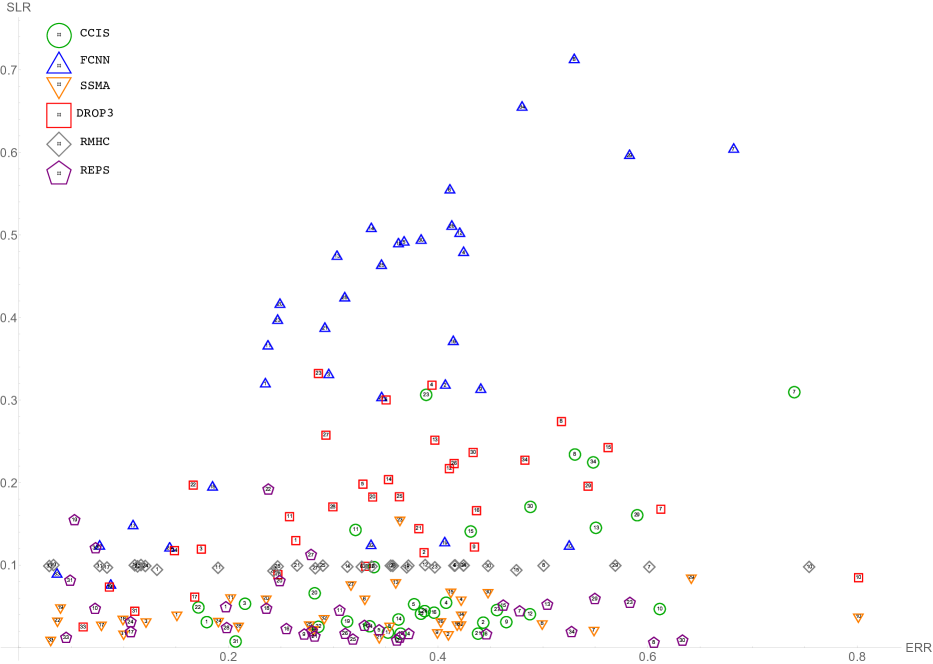
Figure 1: Error and Selection Rates (Vector Data)

The summary of the performances is presented in Table 2. Each row shows ERR and SLR of each method on one dataset. The selection rate for NoPS, which is always 1, is omitted. The values of algorithms whose Pareto-rank is 1 are indicated in bold. Overall, REPS and SSMA are Pareto-rank 1 in the largest numbers of datasets.

The FSR errors of the proposed algorithm and the error rates of the baselines are presented in Table 3 The even number columns show the FSR errors of REPS using the same selection rate as the baseline in the next column. The odd numbered columns shows the ERR of the baselines. The selection rates of the baseline algorithms are the same as those shown in through 5${}^{\text{th}}$-13${}^{\text{th}}$ columns of Table 2.

Table 3: Summary of FSR Error Rates

REPS CCIS REPS FCNN REPS SSMA REPS DROP3 REPS RMHC appendicitis $\mathbf{0.17}$ 0.18 $\mathbf{0.17}$ 0.24 0.22 $\mathbf{0.15}$ $\mathbf{0.19}$ 0.26 0.19 $\mathbf{0.13}$ australian $\mathbf{0.28}$ 0.44 $\mathbf{0.28}$ 0.41 $\mathbf{0.34}$ 0.41 $\mathbf{0.27}$ 0.39 $\mathbf{0.27}$ 0.42 balance $\mathbf{0.12}$ 0.22 $\mathbf{0.15}$ 0.30 0.21 $\mathbf{0.12}$ $\mathbf{0.14}$ 0.17 0.15 $\mathbf{0.12}$ bands $\mathbf{0.32}$ 0.41 $\mathbf{0.32}$ 0.42 $\mathbf{0.38}$ 0.42 $\mathbf{0.30}$ 0.39 $\mathbf{0.36}$ 0.42 breast $\mathbf{0.33}$ 0.38 $\mathbf{0.32}$ 0.37 0.43 $\mathbf{0.35}$ $\mathbf{0.32}$ 0.33 $\mathbf{0.36}$ 0.37 bupa 0.39 $\mathbf{0.34}$ $\mathbf{0.39}$ 0.41 0.40 $\mathbf{0.33}$ 0.41 $\mathbf{0.35}$ 0.40 $\mathbf{0.33}$ cleveland $\mathbf{0.48}$ 0.74 $\mathbf{0.47}$ 0.68 $\mathbf{0.49}$ 0.55 $\mathbf{0.47}$ 0.61 $\mathbf{0.46}$ 0.60 contraceptive 0.54 $\mathbf{0.53}$ 0.55 $\mathbf{0.53}$ 0.55 $\mathbf{0.50}$ $\mathbf{0.51}$ 0.52 0.52 $\mathbf{0.50}$ crx $\mathbf{0.23}$ 0.47 $\mathbf{0.23}$ 0.44 $\mathbf{0.27}$ 0.40 $\mathbf{0.26}$ 0.44 $\mathbf{0.26}$ 0.42 dermatology $\mathbf{0.076}$ 0.61 $\mathbf{0.070}$ 0.53 $\mathbf{0.076}$ 0.80 $\mathbf{0.076}$ 0.80 $\mathbf{0.076}$ 0.75 ecoli $\mathbf{0.26}$ 0.32 0.27 $\mathbf{0.24}$ 0.27 $\mathbf{0.20}$ 0.26 $\mathbf{0.26}$ 0.27 $\mathbf{0.19}$ german $\mathbf{0.32}$ 0.49 $\mathbf{0.32}$ 0.42 $\mathbf{0.34}$ 0.42 $\mathbf{0.31}$ 0.41 $\mathbf{0.30}$ 0.39 glass $\mathbf{0.36}$ 0.55 0.34 $\mathbf{0.30}$ 0.48 $\mathbf{0.36}$ 0.42 $\mathbf{0.40}$ 0.48 $\mathbf{0.36}$ haberman 0.36 $\mathbf{0.36}$ 0.35 $\mathbf{0.34}$ 0.34 $\mathbf{0.28}$ $\mathbf{0.32}$ 0.35 0.32 $\mathbf{0.31}$ hayes-roth $\mathbf{0.39}$ 0.43 0.39 $\mathbf{0.36}$ 0.44 $\mathbf{0.41}$ $\mathbf{0.38}$ 0.56 $\mathbf{0.45}$ 0.47 heart $\mathbf{0.20}$ 0.40 $\mathbf{0.19}$ 0.41 $\mathbf{0.21}$ 0.42 $\mathbf{0.20}$ 0.44 $\mathbf{0.21}$ 0.37 housevotes $\mathbf{0.083}$ 0.35 $\mathbf{0.086}$ 0.11 0.11 $\mathbf{0.079}$ $\mathbf{0.094}$ 0.17 0.087 $\mathbf{0.084}$ ionosphere $\mathbf{0.12}$ 0.36 $\mathbf{0.13}$ 0.19 0.26 $\mathbf{0.10}$ $\mathbf{0.21}$ 0.25 0.20 $\mathbf{0.11}$ iris $\mathbf{0.073}$ 0.31 $\mathbf{0.1}$ 0.41 0.13 $\mathbf{0.040}$ 0.1 $\mathbf{0.087}$ 0.087 $\mathbf{0.033}$ lymphography $\mathbf{0.21}$ 0.28 $\mathbf{0.22}$ 0.25 0.24 $\mathbf{0.24}$ $\mathbf{0.23}$ 0.34 0.26 $\mathbf{0.24}$ mammographic $\mathbf{0.21}$ 0.44 $\mathbf{0.21}$ 0.29 $\mathbf{0.30}$ 0.34 $\mathbf{0.21}$ 0.38 $\mathbf{0.23}$ 0.27 monk-2 0.18 $\mathbf{0.17}$ 0.16 $\mathbf{0.088}$ 0.25 $\mathbf{0.037}$ 0.17 $\mathbf{0.17}$ 0.19 $\mathbf{0.11}$ movement$\_$libras $\mathbf{0.32}$ 0.39 0.32 $\mathbf{0.25}$ $\mathbf{0.35}$ 0.36 0.34 $\mathbf{0.29}$ $\mathbf{0.39}$ 0.40 newthyroid $\mathbf{0.079}$ 0.33 $\mathbf{0.12}$ 0.14 $\mathbf{0.11}$ 0.19 $\mathbf{0.084}$ 0.15 $\mathbf{0.098}$ 0.12 pima $\mathbf{0.29}$ 0.38 $\mathbf{0.29}$ 0.35 $\mathbf{0.27}$ 0.28 $\mathbf{0.26}$ 0.36 $\mathbf{0.27}$ 0.29 saheart $\mathbf{0.37}$ 0.39 $\mathbf{0.38}$ 0.41 $\mathbf{0.29}$ 0.40 $\mathbf{0.31}$ 0.42 $\mathbf{0.29}$ 0.36 sonar $\mathbf{0.20}$ 0.46 $\mathbf{0.20}$ 0.35 0.33 $\mathbf{0.32}$ $\mathbf{0.21}$ 0.29 0.33 $\mathbf{0.28}$ spectfheart $\mathbf{0.23}$ 1.0 $\mathbf{0.23}$ 0.31 $\mathbf{0.20}$ 0.21 $\mathbf{0.21}$ 0.30 $\mathbf{0.20}$ 0.25 tae $\mathbf{0.50}$ 0.59 $\mathbf{0.49}$ 0.58 $\mathbf{0.51}$ 0.64 $\mathbf{0.53}$ 0.54 $\mathbf{0.54}$ 0.57 vehicle $\mathbf{0.30}$ 0.49 $\mathbf{0.34}$ 0.38 $\mathbf{0.38}$ 0.45 $\mathbf{0.36}$ 0.43 $\mathbf{0.38}$ 0.45 wdbc $\mathbf{0.044}$ 0.21 $\mathbf{0.060}$ 0.077 0.11 $\mathbf{0.10}$ $\mathbf{0.072}$ 0.11 $\mathbf{0.049}$ 0.077 wine $\mathbf{0.056}$ 0.29 $\mathbf{0.051}$ 0.34 $\mathbf{0.062}$ 0.29 $\mathbf{0.062}$ 0.33 $\mathbf{0.062}$ 0.34 wisconsin $\mathbf{0.032}$ 1.0 $\mathbf{0.031}$ 0.037 0.044 $\mathbf{0.031}$ $\mathbf{0.048}$ 0.062 $\mathbf{0.029}$ 0.029 yeast $\mathbf{0.48}$ 0.55 0.48 $\mathbf{0.48}$ 0.46 $\mathbf{0.42}$ $\mathbf{0.45}$ 0.48 0.46 $\mathbf{0.42}$

We tested the significance of the differences in the two experimental results, using Wilcoxon’s signed rank tests. The Pareto-ranks of respective algorithms based the error and selection rates from Table 2 were compared with that of REPS with the alternative hypothesis that the average for REPS is smaller. For comparing the FSR errors, the values from the adjacent, corresponding columns in Table 3 were taken and tested, respectively.

The summary of the tests are shown in Table 4. The first and the second rows show the $p$-values from the comparisons of the Pareto-ranks and the FSR errors, respectively. In the Pareto-ranks comparison test, the null hypotheses for all baselines but SSMA can be rejected with a high confidence. For the comparison of FSR errors, the null hypotheses for baselines other than SSMA and RMHC can be rejected with a high confidence. SSMA and RMHC were two best algorithms in [13], which indicates that REPS has a significant advantage against many prototype selection algorithms and is competitive with the state-of-the-art.

Table 4: Summary of the Signed Rank Tests

CCIS FCNN SSMA DROP3 RMHC PARETO 0.00019 4.6 $\times 10^{-6}$ 0.36 1.1$\times 10^{-6}$ 0.00043 FSR ERR 7.1$\times 10^{-7}$ 0.00011 0.39 9.6$\times 10^{-6}$ 0.11

6 Conclusion

This paper presented an extension of the nearest neighbor rule based on the adjustment of ranks to parametrize the prototype selection problem and also to approximate the violation of the rule over the training set. As a result, the problem is defined as discriminative learning in a sparse feature space. Our empirical results showed that it is competitive with the state-of-the-art prototype selection algorithm has the advantage over many other existing algorithms in multiple-measure comparisons.

References

- [1] J. Alcalà-Fdez, L. Sánchez, S. García, M. del Jesus, S. Ventura, J. Garrell, J. Otero, C. Romero, J. Bacardit, V. Rivas, J. Fernández, and F. Herrera, Keel: a software tool to assess evolutionary algorithms for data mining problems, Soft Computing, 13 (2009), pp. 307–318https://doi.org/10.1007/s00500-008-0323-yhttp://dx.doi.org/10.1007/s00500-008-0323-y.
- [2] A. Andoni and P. Indyk, Near-optimal hashing algorithms for approximate nearest neighbor in high dimensions, Commun. ACM, 51 (2008), pp. 117–122https://doi.org/10.1145/1327452.1327494http://doi.acm.org/10.1145/1327452.1327494.
- [3] F. Angiulli, Fast nearest neighbor condensation for large data sets classification, IEEE Trans. on Knowl. and Data Eng., 19 (2007), pp. 1450–1464https://doi.org/10.1109/TKDE.2007.190645http://dx.doi.org/10.1109/TKDE.2007.190645.
- [4] K. Bache and M. Lichman, UCI Machine Learning Repository. archive.ics.uci.edu/ml, 2013.
- [5] D. J. Berndt and J. Clifford, Using Dynamic Time Warping to Find Patterns in Time Series, in Proceedings of KDD-94: AAAI Workshop on Knowledge Discovery in Databases, Seattle, Washington, July 1994, pp. 359–370.
- [6] S. Boyd and L. Vandenberghe, Convex Optimization, Cambridge University Press, New York, NY, USA, 2004.
- [7] H. Brighton and C. Mellish, Advances in instance selection for instance-based learning algorithms, Data Min. Knowl. Discov., 6 (2002), pp. 153–172https://doi.org/10.1023/A:1014043630878http://dx.doi.org/10.1023/A:1014043630878.
- [8] Y. Chen, E. Keogh, B. Hu, N. Begum, A. Bagnall, A. Mueen, and G. Batista, UCR time series classification archive, 2015www.cs.ucr.edu/~eamonn/time_series_data/.
- [9] K. Deb, A. Pratap, S. Agarwal, and T. Meyarivan, A fast and elitist multiobjective genetic algorithm: NSGA-II, IEEE Trans. on Evolut. Comput., 6 (2002), pp. 182–197.
- [10] J. Demšar, Statistical comparisons of classifiers over multiple data sets, J. Mach. Learn. Res., 7 (2006), pp. 1–30http://dl.acm.org/citation.cfm?id=1248547.1248548.
- [11] H. Ding, G. Trajcevski, P. Scheuermann, X. Wang, and E. Keogh, Querying and mining of time series data: Experimental comparison of representations and distance measures, Proc. VLDB Endow., 1 (2008), pp. 1542–1552https://doi.org/10.14778/1454159.1454226http://dx.doi.org/10.14778/1454159.1454226.
- [12] H. A. Fayed and A. F. Atiya, A novel template reduction approach for the k-nearest neighbor method, Trans. Neur. Netw., 20 (2009), pp. 890–896https://doi.org/10.1109/TNN.2009.2018547http://dx.doi.org/10.1109/TNN.2009.2018547.
- [13] S. Garcia, J. Derrac, J. Cano, and F. Herrera, Prototype selection for nearest neighbor classification: Taxonomy and empirical study, IEEE Trans. Pattern Anal. Mach. Intell., 34 (2012), pp. 417–435https://doi.org/10.1109/TPAMI.2011.142http://dx.doi.org/10.1109/TPAMI.2011.142.
- [14] N. García-Pedrajas, Constructing ensembles of classifiers by means of weighted instance selection, Trans. Neur. Netw., 20 (2009), pp. 258–277https://doi.org/10.1109/TNN.2008.2005496http://dx.doi.org/10.1109/TNN.2008.2005496.
- [15] N. García-Pedrajas and A. De Haro-García, Boosting instance selection algorithms, Know.-Based Syst., 67 (2014), pp. 342–360https://doi.org/10.1016/j.knosys.2014.04.021http://dx.doi.org/10.1016/j.knosys.2014.04.021.
- [16] T. Graepel, R. Herbrich, P. Bollmann-Sdorra, and K. Obermayer, Classification on pairwise proximity data, in Proceedings of the 11th International Conference on Neural Information Processing Systems, NIPS’98, 1998, pp. 438–444http://dl.acm.org/citation.cfm?id=3009055.3009117.
- [17] T. Joachims, T. Finley, and C.-N. J. Yu, Cutting-plane Training of Structural SVMs, Mach. Learn., 77 (2009), pp. 27–59https://doi.org/10.1007/s10994-009-5108-8http://dl.acm.org/citation.cfm?id=1612990.1613006.
- [18] C. Kelley, Iterative Methods for Optimization, Frontiers in Applied Mathematics, Society for Industrial and Applied Mathematics, 1999https://books.google.co.jp/books?id=Bq6VcmzOe1IC.
- [19] E. Marchiori, Class conditional nearest neighbor for large margin instance selection, IEEE Trans. Pattern Anal. Mach. Intell., 32 (2010), pp. 364–370https://doi.org/10.1109/TPAMI.2009.164http://dx.doi.org/10.1109/TPAMI.2009.164.
- [20] P. Nemenyi, Distribution-free multiple comparisons, PhD thesis, Princeton University, 1963.
- [21] R. T. Olszewski, Generalized Feature Extraction for Structural Pattern Recognition in Time-series Data, PhD thesis, Carnegie Mellon University, Pittsburgh, PA, USA, 2001. AAI3040489.
- [22] J. A. Olvera-López, J. A. Carrasco-Ochoa, J. F. Martínez-Trinidad, and J. Kittler, A review of instance selection methods, Artif. Intell. Rev., 34 (2010), pp. 133–143https://doi.org/10.1007/s10462-010-9165-yhttp://dx.doi.org/10.1007/s10462-010-9165-y.
- [23] L. Paulevé, H. Jégou, and L. Amsaleg, Locality sensitive hashing: A comparison of hash function types and querying mechanisms, Pattern Recogn. Lett., 31 (2010), pp. 1348–1358https://doi.org/10.1016/j.patrec.2010.04.004http://dx.doi.org/10.1016/j.patrec.2010.04.004.
- [24] E. Pkalska, R. P. W. Duin, and P. Paclík, Prototype selection for dissimilarity-based classifiers, Pattern Recogn., 39 (2006), pp. 189–208.
- [25] D. B. Skalak, Prototype and feature selection by sampling and random mutation hill climbing algorithms, in Proceedings of the Eleventh International Conference on Machine Learning, 1994, pp. 293–301.
- [26] W. S. Torgerson, Multidimensional scaling of similarity, Psychometrika, 30 (1965), pp. 379–393.
- [27] I. Triguero, J. Derrac, S. Garcia, and F. Herrera, A taxonomy and experimental study on prototype generation for nearest neighbor classification, Trans. Sys. Man Cyber Part C, 42 (2012), pp. 86–100https://doi.org/10.1109/TSMCC.2010.2103939http://dx.doi.org/10.1109/TSMCC.2010.2103939.
- [28] D. R. Wilson and T. R. Martinez, Reduction techniques for instance-basedlearning algorithms, Mach. Learn., 38 (2000), pp. 257–286https://doi.org/10.1023/A:1007626913721http://dx.doi.org/10.1023/A:1007626913721.
- [29] X. Wu and V. Kumar, The Top Ten Algorithms in Data Mining, Chapman & Hall/CRC, 1st ed., 2009.