Moss: A Scalable Tool for Efficiently Sampling and Counting 4- and 5-Node Graphlets

Pinghui Wang    Jing Tao    Junzhou Zhao    and Xiaohong Guan

{phwang, jtao, jzzhao, xhguan}@sei.xjtu.edu.cn
MOE Key Laboratory for Intelligent Networks and Network Security, Xi’an Jiaotong University, China
Abstract

Counting the frequencies of 3-, 4-, and 5-node undirected motifs (also know as graphlets) is widely used for understanding complex networks such as social and biology networks. However, it is a great challenge to compute these metrics for a large graph due to the intensive computation. Despite recent efforts to count triangles (i.e., 3-node undirected motif counting), little attention has been given to developing scalable tools that can be used to characterize 4- and 5-node motifs. In this paper, we develop computational efficient methods to sample and count 4- and 5- node undirected motifs. Our methods provide unbiased estimators of motif frequencies, and we derive simple and exact formulas for the variances of the estimators. Moreover, our methods are designed to fit vertex centric programming models, so they can be easily applied to current graph computing systems such as Pregel and GraphLab. We conduct experiments on a variety of real-word datasets, and experimental results show that our methods are several orders of magnitude faster than the state-of-the-art methods under the same estimation errors.

1 Introduction

Refer to caption
(a) 4-node undirected motifs Mi(4),1i6superscriptsubscript𝑀𝑖41𝑖6M_{i}^{(4)},1\leq i\leq 6.
Refer to caption
(b) 5-node undirected motifs Mi(5),1i21superscriptsubscript𝑀𝑖51𝑖21M_{i}^{(5)},1\leq i\leq 21.
Figure 1: The 4- and 5-node motifs studied in this paper.

Design tools for counting the frequencies of the appearance of 3-, 4-, and 5-node connected subgraph patterns (i.e., motifs, also known as graphlets) in a graph is important for understanding and exploring networks such as online social networks and computer networks. For example, a variety of motif-based network analysis techniques have been widely used to characterize communication and evolution patterns in OSNs [6, 15, 33, 28], Internet traffic classification and anomaly detection [13, 8], pattern recognition in gene expression profiling [26], protein-protein interaction predication [2], and coarse-grained topology generation [9].

Due to combinatorial explosion, it is computational intensive to enumerate and count motif frequencies even for a moderately sized graph. For example, medium-size networks Slashdot [18] and Epinions [24] have 105superscript10510^{5} nodes and 106superscript10610^{6} edges but have more than 1010superscript101010^{10} 4-node connected and induced subgraphs (CISes) [29]. To address this problem, cheaper methods such as sampling can be used rather than the brute-force enumeration method. Unfortunately, existing methods of estimating motif concentrations [14, 31, 4, 29, 30] cannot be used to estimate motif frequencies, which are more fundamental than motif concentrations.

Despite recent efforts to count triangles [27, 22, 10, 1], little attention has been given to developing scalable tools that can be used to characterize 4- and 5-node motifs. Jha et al. [11] develop sampling methods to estimate 4-node undirected motifs’ frequencies. In our experiment we observe that their methods do not bound the estimation error tightly, so they significantly over-estimate the sampling budget required to achieve a certain accuracy. Meanwhile, their methods cannot be easily extended to characterize 5-node undirected motifs. Moreover, their methods use an edge-centric program model, so it is difficult to implement them on current graph computing systems such as Pregel [20], GraphLab [19] and GraphChi [16]. In this paper, we propose new methods to estimate the frequencies of 4- and 5-node motifs. Our contributions are summarized as: 1) Our methods of sampling 4- and 5-node motifs are computational efficient and scalable. Meanwile, they can be easily implemented via vertex centric programming models, which are required by most current graph computing systems. 2) To validate our methods, we perform an in-depth analysis. We find that our methods provide unbiased estimators of motif frequencies. To the best of our knowledge, we are the first to derive simple and exact formulas for the variances of the estimators, which is critical for determining a proper sampling budget in practice. Moreover, we conduct experiments on a variety of publicly available datasets, and experimental results show that our methods significantly outperform the state-of-the-art methods.

The rest of this paper is organized as follows. The problem formulation is presented in Section 2. Section 3 introduces preliminaries used in this paper. Section 4 presents our 4- and 5-node motif sampling methods. The performance evaluation and testing results are presented in Section 6. Section 7 summarizes related work. Concluding remarks then follow.

2 Problem Formulation

Let G=(V,E)𝐺𝑉𝐸G=(V,E) be the undirected graph of interest, where V𝑉V and E𝐸E are the sets of nodes and edges respectively. To formally define 4- and 5-node motif frequencies of G𝐺G, we first introduce some notations. An induced subgraph of G𝐺G, G=(V,E)superscript𝐺superscript𝑉superscript𝐸G^{\prime}=(V^{\prime},E^{\prime}), is a subgraph whose edges are all in G𝐺G, i.e. VVsuperscript𝑉𝑉V^{\prime}\subset V, E={(u,v):u,vV,(u,v)E}superscript𝐸conditional-set𝑢𝑣formulae-sequence𝑢𝑣superscript𝑉𝑢𝑣𝐸E^{\prime}=\{(u,v):u,v\in V^{\prime},(u,v)\in E\}. We would like to point out that if we do not say “induced" in this paper, we mean that a subgraph is not necessarily induced. Fig. 1(a) shows all 4-node motifs M1(4),,M6(4)superscriptsubscript𝑀14superscriptsubscript𝑀64M_{1}^{(4)},\ldots,M_{6}^{(4)} of any undirected network. Denote Ci(4)superscriptsubscript𝐶𝑖4C_{i}^{(4)} as the set of 4-node CISes in G𝐺G isomorphic to motif Mi(4)superscriptsubscript𝑀𝑖4M_{i}^{(4)}, and then the motif frequency of Mi(4)superscriptsubscript𝑀𝑖4M_{i}^{(4)} is defined as ni=|Ci(4)|subscript𝑛𝑖superscriptsubscript𝐶𝑖4n_{i}=|C_{i}^{(4)}|, 1i61𝑖61\leq i\leq 6. Fig. 1(b) shows all 5-node motifs M1(5),,M21(5)superscriptsubscript𝑀15superscriptsubscript𝑀215M_{1}^{(5)},\ldots,M_{21}^{(5)} of any undirected network. Denote Ci(5)superscriptsubscript𝐶𝑖5C_{i}^{(5)} as the set of 5-node CISes in G𝐺G isomorphic to motif Mi(5)superscriptsubscript𝑀𝑖5M_{i}^{(5)}, and then the motif frequency of Mi(5)superscriptsubscript𝑀𝑖5M_{i}^{(5)} is defined as ηi=|Ci(5)|subscript𝜂𝑖superscriptsubscript𝐶𝑖5\eta_{i}=|C_{i}^{(5)}|, 1i211𝑖211\leq i\leq 21. In this paper, we aim to develop computational methods to estimate n1,,n6subscript𝑛1subscript𝑛6n_{1},\ldots,n_{6} and η1,,η21subscript𝜂1subscript𝜂21\eta_{1},\ldots,\eta_{21}. For ease of reading, we list notations used throughout the paper in Table 1 and we present the proofs of all theorems in this paper in Appendix.

Table 1: Table of notations.
G=(V,E)𝐺𝑉𝐸G=(V,E) G𝐺G is the undirected graph of interest.
Nvsubscript𝑁𝑣N_{v} the set of neighbors of a node v𝑣v in G𝐺G
dvsubscript𝑑𝑣d_{v} dv=|Nv|subscript𝑑𝑣subscript𝑁𝑣d_{v}=|N_{v}|
M1(4),,M6(4)superscriptsubscript𝑀14superscriptsubscript𝑀64M_{1}^{(4)},\ldots,M_{6}^{(4)} 4-node undirected motifs
M(4)(s)superscript𝑀4𝑠M^{(4)}(s) 4-node motif class ID of CIS s𝑠s
C1(4),,C6(4)superscriptsubscript𝐶14superscriptsubscript𝐶64C_{1}^{(4)},\ldots,C_{6}^{(4)} Ci(4)superscriptsubscript𝐶𝑖4C_{i}^{(4)} as the set of 4-node CISes in G𝐺G
isomorphic to motif Mi(4)superscriptsubscript𝑀𝑖4M_{i}^{(4)}, 1i61𝑖61\leq i\leq 6.
n1(4),,n6(4)superscriptsubscript𝑛14superscriptsubscript𝑛64n_{1}^{(4)},\ldots,n_{6}^{(4)} the frequency of motif Mi(4)superscriptsubscript𝑀𝑖4M_{i}^{(4)}, i.e.,
ni=|Ci(4)|subscript𝑛𝑖superscriptsubscript𝐶𝑖4n_{i}=|C_{i}^{(4)}|, 1i61𝑖61\leq i\leq 6.
M1(5),,M21(5)superscriptsubscript𝑀15superscriptsubscript𝑀215M_{1}^{(5)},\ldots,M_{21}^{(5)} 5-node undirected motifs
M(5)(s)superscript𝑀5𝑠M^{(5)}(s) 5-node motif class ID of CIS s𝑠s
C1(5),,C21(5)superscriptsubscript𝐶15superscriptsubscript𝐶215C_{1}^{(5)},\ldots,C_{21}^{(5)} Ci(5)superscriptsubscript𝐶𝑖5C_{i}^{(5)} as the set of 5-node CISes in G𝐺G
isomorphic to motif Mi(5)superscriptsubscript𝑀𝑖5M_{i}^{(5)}, 1i211𝑖211\leq i\leq 21.
η1(5),,η21(5)superscriptsubscript𝜂15superscriptsubscript𝜂215\eta_{1}^{(5)},\ldots,\eta_{21}^{(5)} the frequency of motif Mi(5)superscriptsubscript𝑀𝑖5M_{i}^{(5)}, i.e.,
ηi=|Ci(5)|subscript𝜂𝑖superscriptsubscript𝐶𝑖5\eta_{i}=|C_{i}^{(5)}|, 1i211𝑖211\leq i\leq 21.
Nu,vsubscript𝑁𝑢𝑣N_{u,v} Nu,v={x:xNu, and xv}subscript𝑁𝑢𝑣conditional-set𝑥formulae-sequence𝑥subscript𝑁𝑢succeeds and 𝑥𝑣N_{u,v}=\{x:x\in N_{u},\text{ and }x\succ v\}
du,vsubscript𝑑𝑢𝑣d_{u,v} du,v=|Nu,v|subscript𝑑𝑢𝑣subscript𝑁𝑢𝑣d_{u,v}=|N_{u,v}|
K𝐾K sampling budget of MOSS-4
Kˇˇ𝐾\check{K} sampling budget of MOSS-4Min
K1subscript𝐾1K_{1}, K2subscript𝐾2K_{2} sampling budgets of MOSS-5
ϕi(1),1i21superscriptsubscriptitalic-ϕ𝑖11𝑖21\phi_{i}^{(1)},1\leq i\leq 21 the number of subgraphs in motif Mi(5)superscriptsubscript𝑀𝑖5M_{i}^{(5)}
that are isomorphic to motif M3(5)superscriptsubscript𝑀35M_{3}^{(5)}
ϕi(2),1i21superscriptsubscriptitalic-ϕ𝑖21𝑖21\phi_{i}^{(2)},1\leq i\leq 21 the number of subgraphs in motif Mi(5)superscriptsubscript𝑀𝑖5M_{i}^{(5)}
that are isomorphic to motif M1(5)superscriptsubscript𝑀15M_{1}^{(5)}
ϕi(3),1i21superscriptsubscriptitalic-ϕ𝑖31𝑖21\phi_{i}^{(3)},1\leq i\leq 21 the number of subgraphs in motif Mi(5)superscriptsubscript𝑀𝑖5M_{i}^{(5)}
that are isomorphic to motif M2(5)superscriptsubscript𝑀25M_{2}^{(5)}
Ω1subscriptΩ1\Omega_{1} Ω1={j:ϕj(1)>0}subscriptΩ1conditional-set𝑗superscriptsubscriptitalic-ϕ𝑗10\Omega_{1}=\{j:\phi_{j}^{(1)}>0\}
Ω2subscriptΩ2\Omega_{2} Ω2={j:ϕj(2)>0}subscriptΩ2conditional-set𝑗superscriptsubscriptitalic-ϕ𝑗20\Omega_{2}=\{j:\phi_{j}^{(2)}>0\}
Ω3subscriptΩ3\Omega_{3} Ω3={j:ϕj(3)>0}subscriptΩ3conditional-set𝑗superscriptsubscriptitalic-ϕ𝑗30\Omega_{3}=\{j:\phi_{j}^{(3)}>0\}
Λ3=vV(dv3),Λ4=vV(dv4)formulae-sequencesubscriptΛ3subscript𝑣𝑉binomialsubscript𝑑𝑣3subscriptΛ4subscript𝑣𝑉binomialsubscript𝑑𝑣4\Lambda_{3}=\sum_{v\in V}\binom{d_{v}}{3},\quad\Lambda_{4}=\sum_{v\in V}\binom{d_{v}}{4}
Γ=vV((dv1)xNv(dx1))Γsubscript𝑣𝑉subscript𝑑𝑣1subscript𝑥subscript𝑁𝑣subscript𝑑𝑥1\Gamma=\sum_{v\in V}\left((d_{v}-1)\sum_{x\in N_{v}}(d_{x}-1)\right)
Γˇ=vVxNvdv,xdx,vˇΓsubscript𝑣𝑉subscript𝑥subscript𝑁𝑣subscript𝑑𝑣𝑥subscript𝑑𝑥𝑣\check{\Gamma}=\sum_{v\in V}\sum_{x\in N_{v}}d_{v,x}d_{x,v}
Γ(1)=vV((dv1)(dv2)xNv(dx1))superscriptΓ1subscript𝑣𝑉subscript𝑑𝑣1subscript𝑑𝑣2subscript𝑥subscript𝑁𝑣subscript𝑑𝑥1\Gamma^{(1)}=\sum_{v\in V}\left((d_{v}-1)(d_{v}-2)\sum_{x\in N_{v}}(d_{x}-1)\right)
Γ(2)=vV((xNv(dx1))2xNv(dx1)2)superscriptΓ2subscript𝑣𝑉superscriptsubscript𝑥subscript𝑁𝑣subscript𝑑𝑥12subscript𝑥subscript𝑁𝑣superscriptsubscript𝑑𝑥12\Gamma^{(2)}=\sum_{v\in V}\left(\left(\sum_{x\in N_{v}}(d_{x}-1)\right)^{2}-\sum_{x\in N_{v}}(d_{x}-1)^{2}\right)

3 Preliminaries

3.1 Mix Unbiased Estimators

Theorem 1

Suppose we have n𝑛n unbiased estimates c1,,cnsubscript𝑐1subscript𝑐𝑛c_{1},\ldots,c_{n} of c𝑐c, i.e., 𝔼(c^i)=c,i=1,,nformulae-sequence𝔼subscript^𝑐𝑖𝑐𝑖1𝑛\mathbb{E}(\hat{c}_{i})=c,i=1,\ldots,n. When these estimates are independent and their variances are Var(ci)Varsubscript𝑐𝑖\text{Var}(c_{i}), 1in1𝑖𝑛1\leq i\leq n. Using all these estimates, we can obtain a more accurate unbiased estimate c^^𝑐\hat{c} of c𝑐c by solving

mini=1nαi=1Var(c^)=Var(i=1nαici).subscriptsuperscriptsubscript𝑖1𝑛subscript𝛼𝑖1Var^𝑐Varsuperscriptsubscript𝑖1𝑛subscript𝛼𝑖subscript𝑐𝑖\min_{\sum_{i=1}^{n}\alpha_{i}=1}\text{Var}(\hat{c})=\text{Var}(\sum_{i=1}^{n}\alpha_{i}c_{i}).

We can easily obtain the optimal Var(c^)=1j=1nVar1(cj)Var^𝑐1superscriptsubscript𝑗1𝑛superscriptVar1subscript𝑐𝑗\text{Var}(\hat{c})=\frac{1}{\sum_{j=1}^{n}\text{Var}^{-1}(c_{j})} when αi=Var1(ci)j=1nVar1(cj)subscript𝛼𝑖superscriptVar1subscript𝑐𝑖superscriptsubscript𝑗1𝑛superscriptVar1subscript𝑐𝑗\alpha_{i}=\frac{\text{Var}^{-1}(c_{i})}{\sum_{j=1}^{n}\text{Var}^{-1}(c_{j})}. We can also estimate the confidence interval of c^^𝑐\hat{c} by the Central Limit Theorem. That is, as n+𝑛n\rightarrow+\infty, for any β>0𝛽0\beta>0, we have

Pr(|c^c|εVar(c^))12πε+et22𝑑teε222πε.Pr^𝑐𝑐𝜀Var^𝑐12𝜋superscriptsubscript𝜀superscript𝑒superscript𝑡22differential-d𝑡superscript𝑒superscript𝜀222𝜋𝜀\text{Pr}\left(|\hat{c}-c|\geq\varepsilon\sqrt{\text{Var}(\hat{c})}\right)\rightarrow\frac{1}{\sqrt{2\pi}}\int_{\varepsilon}^{+\infty}e^{-\frac{t^{2}}{2}}dt\approx\frac{e^{-\frac{\varepsilon^{2}}{2}}}{\sqrt{2\pi}\varepsilon}.

3.2 3-Path Sampling Methods

To describe the state-of-the-art 4-node motif sampling methods: 3-path sampling and centered 3-path sampling [11], we first introduce some notations. Let Nvsubscript𝑁𝑣N_{v} be the set of neighbors of a node vV𝑣𝑉v\in V in G𝐺G. Denote the degree of v𝑣v as dvsubscript𝑑𝑣d_{v}, which is defined as the number of neighbors of v𝑣v in G𝐺G, i.e., dv=|Nv|subscript𝑑𝑣subscript𝑁𝑣d_{v}=|N_{v}|. Let succeeds\succ be a total order on all of the nodes in V𝑉V, which can be easily defined and obtained. For example, suppose we order all nodes based on their degrees and node IDs, and we define uvsucceeds𝑢𝑣u\succ v if du>dvsubscript𝑑𝑢subscript𝑑𝑣d_{u}>d_{v} or, if du=dvsubscript𝑑𝑢subscript𝑑𝑣d_{u}=d_{v} while the node ID of u𝑢u is large than that of v𝑣v. Let Nu,vsubscript𝑁𝑢𝑣N_{u,v} denote the set of u𝑢u’s neighbors with order larger than v𝑣v, i.e.,

Nu,v={x:xNu, and xv}.subscript𝑁𝑢𝑣conditional-set𝑥formulae-sequence𝑥subscript𝑁𝑢succeeds and 𝑥𝑣N_{u,v}=\{x:x\in N_{u},\text{ and }x\succ v\}.

Denote du,v=|Nu,v|subscript𝑑𝑢𝑣subscript𝑁𝑢𝑣d_{u,v}=|N_{u,v}|.

To sample a 4-node CIS, the 3-PATH sampling method mainly consists of five steps: 1) Sample an edge e=(u,v)𝑒𝑢𝑣e=(u,v) from E𝐸E according to the distribution

{π(u,v)=(du1)(dv1)(u,v)E(du1)(dv1):(u,v)E},conditional-setsubscript𝜋𝑢𝑣subscript𝑑𝑢1subscript𝑑𝑣1subscriptsuperscript𝑢superscript𝑣𝐸subscript𝑑superscript𝑢1subscript𝑑superscript𝑣1𝑢𝑣𝐸\{\pi_{(u,v)}=\frac{(d_{u}-1)(d_{v}-1)}{\sum_{(u^{\prime},v^{\prime})\in E}(d_{u^{\prime}}-1)(d_{v^{\prime}}-1)}:(u,v)\in E\},

i.e., the probability of sampling an edge (u,v)E𝑢𝑣𝐸(u,v)\in E is π(u,v)subscript𝜋𝑢𝑣\pi_{(u,v)}; 2) Sample a node w𝑤w from Nv{u}subscript𝑁𝑣𝑢N_{v}-\{u\} uniformly at random; 3) Sample a node r𝑟r from Nu{v}subscript𝑁𝑢𝑣N_{u}-\{v\} uniformly at random; 4) Retrieve the CIS s𝑠s including nodes v𝑣v, u𝑢u, w𝑤w, and r𝑟r. Note that s𝑠s might be a 3-node CIS when r=w𝑟𝑤r=w.

Compared to 3-path sampling, centered 3-path sampling is tailored to estimate the frequencies of 4-node motifs M3(4)superscriptsubscript𝑀34M_{3}^{(4)}, M5(4)superscriptsubscript𝑀54M_{5}^{(4)}, and M6(4)superscriptsubscript𝑀64M_{6}^{(4)}, which are usually not frequently appeared in many real networks. To sample a 4-node CIS, the centered 3-PATH sampling method mainly consists of five steps: 1) Sample an edge e=(u,v)𝑒𝑢𝑣e=(u,v) from E𝐸E according to the distribution

{π(u,v)=du,vdv,u(u,v)Edu,vdv,u:(u,v)E};conditional-setsubscript𝜋𝑢𝑣subscript𝑑𝑢𝑣subscript𝑑𝑣𝑢subscriptsuperscript𝑢superscript𝑣𝐸subscript𝑑superscript𝑢superscript𝑣subscript𝑑superscript𝑣superscript𝑢superscript𝑢superscript𝑣𝐸\{\pi_{(u,v)}=\frac{d_{u,v}d_{v,u}}{\sum_{(u^{\prime},v^{\prime})\in E}d_{u^{\prime},v^{\prime}}d_{v^{\prime},u^{\prime}}}:(u^{\prime},v^{\prime})\in E\};

2) Sample a node w𝑤w from Nv,usubscript𝑁𝑣𝑢N_{v,u} at random; 3) Sample a node r𝑟r from Nu,vsubscript𝑁𝑢𝑣N_{u,v} at random; 4) Retrieve the CIS s𝑠s including nodes v𝑣v, u𝑢u, w𝑤w, and r𝑟r. Similarly, s𝑠s might be a 3-node CIS.

3.3 Vertex-Centric Programming Model

Vertex-centric programming models require users to express their algorithms by “thinking like a vertex". Each node contains information about itself and all its immediate neighbors, and the algorithms’ operations are expressed at the level of a single node. For example, the operations of a node in Pregel involve receiving messages from other nodes, updating the state of itself and its edges, and sending messages to other nodes. Vertex-centric models are very easy to program and have been widely used for many graph mining and machine learning algorithms.

4 Sampling 4-Node Motifs

In this section, we introduce our sampling methods: MOSS-4 and MOSS-4Min. MOSS-4 is used to estimate all 4-node motifs’ frequencies. We observe that MOSS-4 might exhibit large errors for characterizing rare motifs (i.e., motifs with low frequencies) for a small sampling budget. In addition to MOSS-4, we also develop a method MOSS-4Min to further reduce the errors for characterizing rare motifs.

4.1 MOSS-4

4.1.1 Sampling

Denote by Γv=(dv1)xNv(dx1)subscriptΓ𝑣subscript𝑑𝑣1subscript𝑥subscript𝑁𝑣subscript𝑑𝑥1\Gamma_{v}=(d_{v}-1)\sum_{x\in N_{v}}(d_{x}-1). We assign a weight ΓvsubscriptΓ𝑣\Gamma_{v} to each node vV𝑣𝑉v\in V. Define Γ=vVΓvΓsubscript𝑣𝑉subscriptΓ𝑣\Gamma=\sum_{v\in V}\Gamma_{v} and πv=ΓvΓsubscript𝜋𝑣subscriptΓ𝑣Γ\pi_{v}=\frac{\Gamma_{v}}{\Gamma}. Our method of sampling a 4-node CIS mainly consists of five steps: 1) Sample a node v𝑣v from V𝑉V according to the distribution π={πv:vV}𝜋conditional-setsubscript𝜋𝑣𝑣𝑉\pi=\{\pi_{v}:v\in V\}; 2) Sample a random node u𝑢u from Nvsubscript𝑁𝑣N_{v} according to the distribution σ(v)={σu(v):uNv}superscript𝜎𝑣conditional-setsuperscriptsubscript𝜎𝑢𝑣𝑢subscript𝑁𝑣\sigma^{(v)}=\{\sigma_{u}^{(v)}:u\in N_{v}\}, where σu(v)superscriptsubscript𝜎𝑢𝑣\sigma_{u}^{(v)} is defined as

σu(v)=du1xNv(dx1),uNv;formulae-sequencesuperscriptsubscript𝜎𝑢𝑣subscript𝑑𝑢1subscript𝑥subscript𝑁𝑣subscript𝑑𝑥1𝑢subscript𝑁𝑣\sigma_{u}^{(v)}=\frac{d_{u}-1}{\sum_{x\in N_{v}}(d_{x}-1)},\quad u\in N_{v}; (1)

3) Sample a node w𝑤w from Nv{u}subscript𝑁𝑣𝑢N_{v}-\{u\} uniformly at random; 4) Sample a node r𝑟r from Nu{v}subscript𝑁𝑢𝑣N_{u}-\{v\} uniformly at random; 5) Retrieve the CIS s𝑠s including nodes v𝑣v, u𝑢u, w𝑤w, and r𝑟r. We set the sampling budget as K𝐾K, i.e., we run the above method K𝐾K times to obtain K𝐾K CISes s1,,sKsubscript𝑠1subscript𝑠𝐾s_{1},\ldots,s_{K}. The pseudo-code of MOSS-4 is shown in Algorithm 1. In Algorithm 1, function WeightRandomVertex(V,π)WeightRandomVertex𝑉𝜋\text{WeightRandomVertex}(V,\pi) returns a node sampled from V𝑉V according to the distribution π={πv:vV}𝜋conditional-setsubscript𝜋𝑣𝑣𝑉\pi=\{\pi_{v}:v\in V\}, function RandomVertex(X)RandomVertex𝑋\text{RandomVertex}(X) returns a node sampled from X𝑋X at random, and function CIS({v,u,w,r})CIS𝑣𝑢𝑤𝑟\text{CIS}(\{v,u,w,r\}) returns the CIS with the node set {v,u,w,r}𝑣𝑢𝑤𝑟\{v,u,w,r\} in G𝐺G.

4.1.2 Estimator

Let φi(1)superscriptsubscript𝜑𝑖1\varphi_{i}^{(1)}, 1i61𝑖61\leq i\leq 6, be the number of subgraphs in motif Mi(4)superscriptsubscript𝑀𝑖4M_{i}^{(4)} that are isomorphic to motif M1(4)superscriptsubscript𝑀14M_{1}^{(4)}. We can easily compute φ1(1)=1superscriptsubscript𝜑111\varphi_{1}^{(1)}=1, φ2(1)=0superscriptsubscript𝜑210\varphi_{2}^{(1)}=0, φ3(1)=4superscriptsubscript𝜑314\varphi_{3}^{(1)}=4, φ4(1)=2superscriptsubscript𝜑412\varphi_{4}^{(1)}=2, φ5(1)=6superscriptsubscript𝜑516\varphi_{5}^{(1)}=6, and φ6(1)=12superscriptsubscript𝜑6112\varphi_{6}^{(1)}=12. To remove the error introduced by sampling, we analyze the bias of MOSS-4 as follows:

Theorem 2

When the sampling budget K=1𝐾1K=1, MOSS-4 samples a CIS sCi(4)𝑠superscriptsubscript𝐶𝑖4s\in C_{i}^{(4)} with probability pi=2φi(1)Γsubscript𝑝𝑖2superscriptsubscript𝜑𝑖1Γp_{i}=\frac{2\varphi_{i}^{(1)}}{\Gamma}, 1i61𝑖61\leq i\leq 6.

/* K𝐾K is the sampling budget. */
input : G=(V,E)𝐺𝑉𝐸G=(V,E) and K𝐾K.
output : n^isubscript^𝑛𝑖\hat{n}_{i}, 1i61𝑖61\leq i\leq 6.
for i{1,3,4,5,6}𝑖13456i\in\{1,3,4,5,6\} do
       n^i0subscript^𝑛𝑖0\hat{n}_{i}\leftarrow 0;
      
end for
for k[1,K]𝑘1𝐾k\in[1,K] do
       vWeightRandomVertex(V,π)𝑣WeightRandomVertex𝑉𝜋v\leftarrow\textnormal{{WeightRandomVertex}}(V,\pi);
       uWeightRandomVertex(Nv,σ(v))𝑢WeightRandomVertexsubscript𝑁𝑣superscript𝜎𝑣u\leftarrow\textnormal{{WeightRandomVertex}}(N_{v},\sigma^{(v)});
       wRandomVertex(Nv{u})𝑤RandomVertexsubscript𝑁𝑣𝑢w\leftarrow\textnormal{{RandomVertex}}(N_{v}-\{u\});
       rRandomVertex(Nu{v})𝑟RandomVertexsubscript𝑁𝑢𝑣r\leftarrow\textnormal{{RandomVertex}}(N_{u}-\{v\});
       skCIS({v,u,w,r})subscript𝑠𝑘CIS𝑣𝑢𝑤𝑟s_{k}\leftarrow\textnormal{{CIS}}(\{v,u,w,r\});
       if ru𝑟𝑢r\neq u and rw𝑟𝑤r\neq w then
             iM(4)(sk)𝑖superscript𝑀4subscript𝑠𝑘i\leftarrow M^{(4)}(s_{k});
             n^in^i+1Kpisubscript^𝑛𝑖subscript^𝑛𝑖1𝐾subscript𝑝𝑖\hat{n}_{i}\leftarrow\hat{n}_{i}+\frac{1}{Kp_{i}};
            
       end if
      
end for
n^2Λ3n^42n^54n^6subscript^𝑛2subscriptΛ3subscript^𝑛42subscript^𝑛54subscript^𝑛6\hat{n}_{2}\leftarrow\Lambda_{3}-\hat{n}_{4}-2\hat{n}_{5}-4\hat{n}_{6};
Algorithm 1 The pseudo-code of MOSS-4.

We let M(4)(sk)superscript𝑀4subscript𝑠𝑘M^{(4)}(s_{k}) be the 4-node motif class ID of sksubscript𝑠𝑘s_{k} when sksubscript𝑠𝑘s_{k} is a 4-node CIS, and -1 otherwise (i.e., sksubscript𝑠𝑘s_{k} is a triangle). Let 𝟏(𝕏)1𝕏\mathbf{1}(\mathbb{X}) denote the indicator function that equals one when predicate 𝕏𝕏\mathbb{X} is true, and zero otherwise. Denote mi=k=1K𝟏(M(4)(sk)=i)subscript𝑚𝑖superscriptsubscript𝑘1𝐾1superscript𝑀4subscript𝑠𝑘𝑖m_{i}=\sum_{k=1}^{K}\mathbf{1}(M^{(4)}(s_{k})=i). For i{1,3,4,5,6}𝑖13456i\in\{1,3,4,5,6\}, pisubscript𝑝𝑖p_{i} is larger than zero and we estimate nisubscript𝑛𝑖n_{i} as

n^i=miKpi,i{1,3,4,5,6}.formulae-sequencesubscript^𝑛𝑖subscript𝑚𝑖𝐾subscript𝑝𝑖𝑖13456\hat{n}_{i}=\frac{m_{i}}{Kp_{i}},\quad i\in\{1,3,4,5,6\}.

Let Λ3=vV(dv3)subscriptΛ3subscript𝑣𝑉binomialsubscript𝑑𝑣3\Lambda_{3}=\sum_{v\in V}\binom{d_{v}}{3}. Then, the number of all 4-node subgraphs (not necessarily induced) in G𝐺G isomorphic to motif M2(4)superscriptsubscript𝑀24M_{2}^{(4)} is Λ3subscriptΛ3\Lambda_{3}. Let φi(2)superscriptsubscript𝜑𝑖2\varphi_{i}^{(2)}, 1i61𝑖61\leq i\leq 6, be the number of subgraphs in motif Mi(4)superscriptsubscript𝑀𝑖4M_{i}^{(4)} that are isomorphic to motif M2(4)superscriptsubscript𝑀24M_{2}^{(4)}. We have φ1(2)=0superscriptsubscript𝜑120\varphi_{1}^{(2)}=0, φ2(2)=1superscriptsubscript𝜑221\varphi_{2}^{(2)}=1, φ3(2)=0superscriptsubscript𝜑320\varphi_{3}^{(2)}=0, φ4(2)=1superscriptsubscript𝜑421\varphi_{4}^{(2)}=1, φ5(2)=2superscriptsubscript𝜑522\varphi_{5}^{(2)}=2, and φ6(2)=4superscriptsubscript𝜑624\varphi_{6}^{(2)}=4. We can easily find that

Λ3=i=16φi(2)ni=n2+n4+2n5+4n6.subscriptΛ3superscriptsubscript𝑖16superscriptsubscript𝜑𝑖2subscript𝑛𝑖subscript𝑛2subscript𝑛42subscript𝑛54subscript𝑛6\Lambda_{3}=\sum_{i=1}^{6}\varphi_{i}^{(2)}n_{i}=n_{2}+n_{4}+2n_{5}+4n_{6}. (2)

Thus, we estimate n2subscript𝑛2n_{2} as

n^2=Λ3n^42n^54n^6.subscript^𝑛2subscriptΛ3subscript^𝑛42subscript^𝑛54subscript^𝑛6\hat{n}_{2}=\Lambda_{3}-\hat{n}_{4}-2\hat{n}_{5}-4\hat{n}_{6}.
Theorem 3

n^isubscript^𝑛𝑖\hat{n}_{i} is an unbiased estimator of nisubscript𝑛𝑖n_{i}, 1i61𝑖61\leq i\leq 6. The variance of n^isubscript^𝑛𝑖\hat{n}_{i} is

Var(n^i)=niK(1pini),i{1,3,4,5,6}.formulae-sequenceVarsubscript^𝑛𝑖subscript𝑛𝑖𝐾1subscript𝑝𝑖subscript𝑛𝑖𝑖13456\text{Var}(\hat{n}_{i})=\frac{n_{i}}{K}\left(\frac{1}{p_{i}}-n_{i}\right),\quad i\in\{1,3,4,5,6\}.

The variance of n^2subscript^𝑛2\hat{n}_{2} is computed as

Var(n^2)=1K(n4p4+4n5p5+16n6p6(n4+2n5+4n6)2).Varsubscript^𝑛21𝐾subscript𝑛4subscript𝑝44subscript𝑛5subscript𝑝516subscript𝑛6subscript𝑝6superscriptsubscript𝑛42subscript𝑛54subscript𝑛62\text{Var}(\hat{n}_{2})=\frac{1}{K}\left(\frac{n_{4}}{p_{4}}+\frac{4n_{5}}{p_{5}}+\frac{16n_{6}}{p_{6}}-(n_{4}+2n_{5}+4n_{6})^{2}\right).

From Theorem 1, we can easily compute a sampling budget K𝐾K that can guarantee P(|n^ini|>εni)<δ𝑃subscript^𝑛𝑖subscript𝑛𝑖𝜀subscript𝑛𝑖𝛿P(|\hat{n}_{i}-n_{i}|>\varepsilon n_{i})<\delta for any ε>0𝜀0\varepsilon>0 and 0<δ<10𝛿10<\delta<1, i=1,,6𝑖16i=1,\ldots,6.

4.1.3 Computational Complexity

Initialization: For each node v𝑣v, we store its degree dvsubscript𝑑𝑣d_{v} and use a list to store its neighbors Nvsubscript𝑁𝑣N_{v}. Therefore, it requires O(dv)𝑂subscript𝑑𝑣O(d_{v}) operations to compute ΓvsubscriptΓ𝑣\Gamma_{v}, and the computational complexity of processing all nodes is O(|E|)𝑂𝐸O(|E|).

WeightRandomVertex(V,π)WeightRandomVertex𝑉𝜋\text{WeightRandomVertex}(V,\pi): We use a list V[1,,|V|]𝑉1𝑉V[1,\ldots,|V|] to store the nodes in V𝑉V. We store an array ACC_Γ[1,,|V|]𝐴𝐶𝐶_Γ1𝑉ACC\_\Gamma[1,\ldots,|V|] in memory, where ACC_Γ[i]𝐴𝐶𝐶_Γdelimited-[]𝑖ACC\_\Gamma[i] is defined as ACC_Γ[i]=j=1iΓV[j]𝐴𝐶𝐶_Γdelimited-[]𝑖superscriptsubscript𝑗1𝑖subscriptΓ𝑉delimited-[]𝑗ACC\_\Gamma[i]=\sum_{j=1}^{i}\Gamma_{V[j]}, 1i|V|1𝑖𝑉1\leq i\leq|V|. Clearly, ACC_Γ[|V|]=Γ𝐴𝐶𝐶_Γdelimited-[]𝑉ΓACC\_\Gamma[|V|]=\Gamma. Let ACC_Γ[0]=0𝐴𝐶𝐶_Γdelimited-[]00ACC\_\Gamma[0]=0. Then, WeightRandomVertex(V,π)WeightRandomVertex𝑉𝜋\text{WeightRandomVertex}(V,\pi) can be easily achieved by the following three steps:

  • Step 1: Select a number rnd𝑟𝑛𝑑rnd from {1,,Γ}1Γ\{1,\ldots,\Gamma\} at random;

  • Step 2: Find i𝑖i satisfying ACC_Γ[i1]<rndACC_Γ[i]𝐴𝐶𝐶_Γdelimited-[]𝑖1𝑟𝑛𝑑𝐴𝐶𝐶_Γdelimited-[]𝑖ACC\_\Gamma[i-1]<rnd\leq ACC\_\Gamma[i], which can be solved by the binary search algorithm;

  • Step 3: Return V[i]𝑉delimited-[]𝑖V[i].

Its computational complexity is O(log|V|)𝑂𝑉O(\log|V|).

WeightRandomVertex(Nv,σ(v))WeightRandomVertexsubscript𝑁𝑣superscript𝜎𝑣\text{WeightRandomVertex}(N_{v},\sigma^{(v)}): We use a list Nv[1,,dv]subscript𝑁𝑣1subscript𝑑𝑣N_{v}[1,\ldots,d_{v}] to store the neighbors of v𝑣v. We store an array ACC_σ(v)[1,,dv]𝐴𝐶𝐶_superscript𝜎𝑣1subscript𝑑𝑣ACC\_\sigma^{(v)}[1,\ldots,d_{v}] in memory, where ACC_σ(v)[i]𝐴𝐶𝐶_superscript𝜎𝑣delimited-[]𝑖ACC\_\sigma^{(v)}[i] is defined as ACC_σ(v)[i]=j=1i(dNv[j]1)𝐴𝐶𝐶_superscript𝜎𝑣delimited-[]𝑖superscriptsubscript𝑗1𝑖subscript𝑑subscript𝑁𝑣delimited-[]𝑗1ACC\_\sigma^{(v)}[i]=\sum_{j=1}^{i}(d_{N_{v}[j]}-1), 1idv1𝑖subscript𝑑𝑣1\leq i\leq d_{v}. Let ACC_σ(v)[0]=0𝐴𝐶𝐶_superscript𝜎𝑣delimited-[]00ACC\_\sigma^{(v)}[0]=0. Then, WeightRandomVertex(Nv,σ(v))WeightRandomVertexsubscript𝑁𝑣superscript𝜎𝑣\text{WeightRandomVertex}(N_{v},\sigma^{(v)}) can be easily achieved by the following three steps:

  • Step 1: Select a number rnd𝑟𝑛𝑑rnd from {1,,ACC_σ(v)[dv]}1𝐴𝐶𝐶_superscript𝜎𝑣delimited-[]subscript𝑑𝑣\{1,\ldots,ACC\_\sigma^{(v)}[d_{v}]\} at random;

  • Step 2: Find i𝑖i satisfying

    ACC_σ(v)[i1]<rndACC_σ(v)[i],𝐴𝐶𝐶_superscript𝜎𝑣delimited-[]𝑖1𝑟𝑛𝑑𝐴𝐶𝐶_superscript𝜎𝑣delimited-[]𝑖ACC\_\sigma^{(v)}[i-1]<rnd\leq ACC\_\sigma^{(v)}[i],

    which can be solved by the binary search algorithm;

  • Step 3: Return Nv[i]subscript𝑁𝑣delimited-[]𝑖N_{v}[i].

Its computational complexity is O(logdv)𝑂subscript𝑑𝑣O(\log d_{v}).

RandomVertex(Nv{u})RandomVertexsubscript𝑁𝑣𝑢\text{RandomVertex}(N_{v}-\{u\}): Let POSv,u𝑃𝑂subscript𝑆𝑣𝑢POS_{v,u} denote the index of u𝑢u in the list Nv[1,,dv]subscript𝑁𝑣1subscript𝑑𝑣N_{v}[1,\ldots,d_{v}], i.e., Nv[POSv,u]=usubscript𝑁𝑣delimited-[]𝑃𝑂subscript𝑆𝑣𝑢𝑢N_{v}[POS_{v,u}]=u. Then, function RandomVertex(Nv{u})RandomVertexsubscript𝑁𝑣𝑢\text{RandomVertex}(N_{v}-\{u\}) can be achieved by the following steps:

  • Step 1: Select a number rnd𝑟𝑛𝑑rnd from {1,,dv}{POSv,u}1subscript𝑑𝑣𝑃𝑂subscript𝑆𝑣𝑢\{1,\ldots,d_{v}\}-\{POS_{v,u}\} at random;

  • Step 2: Return Nv[rnd]subscript𝑁𝑣delimited-[]𝑟𝑛𝑑N_{v}[rnd].

Its computational complexity is O(1)𝑂1O(1).

In summary, the complexity of MOSS-4 sampling K𝐾K CISes is O(|E|+Klog|V|)𝑂𝐸𝐾𝑉O(|E|+K\log|V|).

4.2 MOSS-4Min

4.2.1 Sampling

From the above derived formulas of the variances of MOSS-4, we can see that MOSS-4 might exhibit larger errors for 4-node motifs with lower frequencies when allocating a small sampling budget K𝐾K. To solve this problem, we develop a better method MOSS-4Min to further reduce the errors for estimating the frequencies of 4-node motifs M3(4)superscriptsubscript𝑀34M_{3}^{(4)}, M5(4)superscriptsubscript𝑀54M_{5}^{(4)}, and M6(4)superscriptsubscript𝑀64M_{6}^{(4)}.

Let Γˇv=xNvdv,xdx,vsubscriptˇΓ𝑣subscript𝑥subscript𝑁𝑣subscript𝑑𝑣𝑥subscript𝑑𝑥𝑣\check{\Gamma}_{v}=\sum_{x\in N_{v}}d_{v,x}d_{x,v}, vV𝑣𝑉v\in V. MOSS-4Min assigns a weight ΓˇvsubscriptˇΓ𝑣\check{\Gamma}_{v} to each node vV𝑣𝑉v\in V. Define Γˇ=vVΓˇvˇΓsubscript𝑣𝑉subscriptˇΓ𝑣\check{\Gamma}=\sum_{v\in V}\check{\Gamma}_{v} and πˇv=ΓˇvΓˇsubscriptˇ𝜋𝑣subscriptˇΓ𝑣ˇΓ\check{\pi}_{v}=\frac{\check{\Gamma}_{v}}{\check{\Gamma}}. MOSS-4Min mainly consists of five steps: 1) Sample a node v𝑣v from V𝑉V according to the distribution πˇ={πˇv:vV}ˇ𝜋conditional-setsubscriptˇ𝜋𝑣𝑣𝑉\check{\pi}=\{\check{\pi}_{v}:v\in V\}. 2) Sample a node u𝑢u from Nvsubscript𝑁𝑣N_{v} according to the distribution σˇ(v)={σˇu(v):uNv}superscriptˇ𝜎𝑣conditional-setsuperscriptsubscriptˇ𝜎𝑢𝑣𝑢subscript𝑁𝑣\check{\sigma}^{(v)}=\{\check{\sigma}_{u}^{(v)}:u\in N_{v}\}, where σˇu(v)superscriptsubscriptˇ𝜎𝑢𝑣\check{\sigma}_{u}^{(v)} is defined as

σˇu(v)=du,vdv,uΓˇv,uNv;formulae-sequencesuperscriptsubscriptˇ𝜎𝑢𝑣subscript𝑑𝑢𝑣subscript𝑑𝑣𝑢subscriptˇΓ𝑣𝑢subscript𝑁𝑣\check{\sigma}_{u}^{(v)}=\frac{d_{u,v}d_{v,u}}{\check{\Gamma}_{v}},\quad u\in N_{v}; (3)

3) Sample a node w𝑤w from Nv,usubscript𝑁𝑣𝑢N_{v,u} at random; 4) Sample a node r𝑟r from Nu,vsubscript𝑁𝑢𝑣N_{u,v} at random; 5) Retrieve the CIS s𝑠s including nodes v𝑣v, u𝑢u, w𝑤w, and r𝑟r. We set the sampling budget as Kˇˇ𝐾\check{K} to obtain Kˇˇ𝐾\check{K} CISes s1,,sKˇsubscript𝑠1subscript𝑠ˇ𝐾s_{1},\ldots,s_{\check{K}}.

4.2.2 Estimator

input : G=(V,E)𝐺𝑉𝐸G=(V,E) and Kˇˇ𝐾\check{K}.
output : nˇisubscriptˇ𝑛𝑖\check{n}_{i}, i{3,5,6}𝑖356i\in\{3,5,6\}.
nˇ30subscriptˇ𝑛30\check{n}_{3}\leftarrow 0, nˇ50subscriptˇ𝑛50\check{n}_{5}\leftarrow 0, and nˇ60subscriptˇ𝑛60\check{n}_{6}\leftarrow 0;
for k[1,Kˇ]𝑘1ˇ𝐾k\in[1,\check{K}] do
       vWeightRandomVertex(V,πˇ)𝑣WeightRandomVertex𝑉ˇ𝜋v\leftarrow\textnormal{{WeightRandomVertex}}(V,\check{\pi});
       uWeightRandomVertex(Nv,σˇ(v))𝑢WeightRandomVertexsubscript𝑁𝑣superscriptˇ𝜎𝑣u\leftarrow\textnormal{{WeightRandomVertex}}(N_{v},\check{\sigma}^{(v)});
       wRandomVertex(Nv,u)𝑤RandomVertexsubscript𝑁𝑣𝑢w\leftarrow\textnormal{{RandomVertex}}(N_{v,u});
       rRandomVertex(Nu,v)𝑟RandomVertexsubscript𝑁𝑢𝑣r\leftarrow\textnormal{{RandomVertex}}(N_{u,v});
       skCIS({v,u,w,r})subscript𝑠𝑘CIS𝑣𝑢𝑤𝑟s_{k}\leftarrow\textnormal{{CIS}}(\{v,u,w,r\});
       if ru𝑟𝑢r\neq u and rw𝑟𝑤r\neq w then
             iM(4)(sk)𝑖superscript𝑀4subscript𝑠𝑘i\leftarrow M^{(4)}(s_{k});
             if i{3,5,6}𝑖356i\in\{3,5,6\} then
                   nˇinˇi+1Kˇpˇisubscriptˇ𝑛𝑖subscriptˇ𝑛𝑖1ˇ𝐾subscriptˇ𝑝𝑖\check{n}_{i}\leftarrow\check{n}_{i}+\frac{1}{\check{K}\check{p}_{i}};
                  
             end if
            
       end if
      
end for
Algorithm 2 The pseudo-code of MOSS-4Min.
Theorem 4

When the sampling budget Kˇ=1ˇ𝐾1\check{K}=1, MOSS-4Min samples CISes sC3(4)𝑠superscriptsubscript𝐶34s\in C_{3}^{(4)}, sC3(5)𝑠superscriptsubscript𝐶35s\in C_{3}^{(5)}, and sC6(4)𝑠superscriptsubscript𝐶64s\in C_{6}^{(4)} with probabilities pˇ3=2Γˇ1subscriptˇ𝑝32superscriptˇΓ1\check{p}_{3}=2\check{\Gamma}^{-1}, pˇ5=2Γˇ1subscriptˇ𝑝52superscriptˇΓ1\check{p}_{5}=2\check{\Gamma}^{-1}, and pˇ6=6Γˇ1subscriptˇ𝑝66superscriptˇΓ1\check{p}_{6}=6\check{\Gamma}^{-1} respectively.

We estimate n3subscript𝑛3n_{3}, n5subscript𝑛5n_{5}, and n6subscript𝑛6n_{6} as

nˇi=k=1KˇmiKˇpˇi,i=3,5,6,formulae-sequencesubscriptˇ𝑛𝑖superscriptsubscript𝑘1ˇ𝐾subscript𝑚𝑖ˇ𝐾subscriptˇ𝑝𝑖𝑖356\check{n}_{i}=\sum_{k=1}^{\check{K}}\frac{m_{i}}{\check{K}\check{p}_{i}},\quad i=3,5,6,

where mi=k=1K𝟏(M(4)(sk)=i)subscript𝑚𝑖superscriptsubscript𝑘1𝐾1superscript𝑀4subscript𝑠𝑘𝑖m_{i}=\sum_{k=1}^{K}\mathbf{1}(M^{(4)}(s_{k})=i). The variances of nˇ3subscriptˇ𝑛3\check{n}_{3}, nˇ5subscriptˇ𝑛5\check{n}_{5}, and nˇ6subscriptˇ𝑛6\check{n}_{6} are given in the following theorem. We omit the proof, which is analogous to that of Theorem 3.

Theorem 5

nˇisubscriptˇ𝑛𝑖\check{n}_{i} is an unbiased estimator of nisubscript𝑛𝑖n_{i}, i=3,5,6𝑖356i=3,5,6. Its variance is

Var(nˇi)=niKˇ(1pˇini),i=3,5,6.formulae-sequenceVarsubscriptˇ𝑛𝑖subscript𝑛𝑖ˇ𝐾1subscriptˇ𝑝𝑖subscript𝑛𝑖𝑖356\text{Var}(\check{n}_{i})=\frac{n_{i}}{\check{K}}\left(\frac{1}{\check{p}_{i}}-n_{i}\right),\quad i=3,5,6.

From Theorems 13, and 5, we can easily obtain a more accurate estimator of nisubscript𝑛𝑖n_{i} by combining n^isubscript^𝑛𝑖\hat{n}_{i} and nˇisubscriptˇ𝑛𝑖\check{n}_{i}, i=3,5,6𝑖356i=3,5,6.

4.2.3 Computational Complexity

We easily extend methods in Section 4.1.3 to design functions WeightRandomVertex(V,πˇ)WeightRandomVertex𝑉ˇ𝜋\text{WeightRandomVertex}(V,\check{\pi}) and WeightRandomVertex(Nv,σˇ(v))WeightRandomVertexsubscript𝑁𝑣superscriptˇ𝜎𝑣\text{WeightRandomVertex}(N_{v},\check{\sigma}^{(v)}) in Algorithm 2. The computational complexity of MOSS-4min sampling K𝐾K CISes is O(|E|+Klog|V|)𝑂𝐸𝐾𝑉O(|E|+K\log|V|).

4.3 Vertex-Centric Programming Models

In this subsection, we show MOSS-4 and MOSS-4MIN can be easily implemented via vertex-centric programming models.

4.3.1 Vertex-Centric Programming Model of MOSS-4 Sampling Method

First, we sample K𝐾K nodes in V𝑉V according to π𝜋\pi. Let kvsubscript𝑘𝑣k_{v} denote the number of times a node vV𝑣𝑉v\in V sampled. Thus, vVkv=Ksubscript𝑣𝑉subscript𝑘𝑣𝐾\sum_{v\in V}k_{v}=K. For each node v𝑣v, we set kvsubscript𝑘𝑣k_{v} as its node value, and then repeat the set of four following operations kvsubscript𝑘𝑣k_{v} times

uWeightRandomVertex(Nv,σ(v)),𝑢WeightRandomVertexsubscript𝑁𝑣superscript𝜎𝑣u\leftarrow\text{WeightRandomVertex}(N_{v},\sigma^{(v)}),
wRandomVertex(Nv{u}),𝑤RandomVertexsubscript𝑁𝑣𝑢w\leftarrow\text{RandomVertex}(N_{v}-\{u\}),
Update(A) and then MSG(v,,w,,A)u,Update𝐴 and then MSG𝑣𝑤𝐴𝑢\text{Update}(A)\text{ and then }\text{MSG}(v,*,w,*,A)\rightarrow u,

where A𝐴A is the adjacent matrix of the CIS consisting of nodes v𝑣v, u𝑢u, w𝑤w, and r𝑟r, which are the variables in the Algorithm 1, i.e., the nodes sampled at the 1-st, 2-nd, 3-rd, and 4-th steps respectively. Note that here r𝑟r and some entries in A𝐴A are unknown. Function Update(A)Update𝐴\text{Update}(A) is used to get the values of unknown entries in A𝐴A based the edges of the current node v𝑣v. Function MSG(v,,w,,A)uMSG𝑣𝑤𝐴𝑢\text{MSG}(v,*,w,*,A)\rightarrow u generates a message (v,,w,,A)𝑣𝑤𝐴(v,*,w,*,A), and sends the message to u𝑢u, which is a neighbor of v𝑣v.

We process the messages that a node receives as follows:

  • When a node u𝑢u receives a message like (v,,w,,A)𝑣𝑤𝐴(v,*,w,*,A), do

    rRandomVertex(Nu{v}),𝑟RandomVertexsubscript𝑁𝑢𝑣r\leftarrow\text{RandomVertex}(N_{u}-\{v\}),
    Update(A) and then MSG(v,u,w,,A)r.Update𝐴 and then MSG𝑣𝑢𝑤𝐴𝑟\text{Update}(A)\text{ and then }\text{MSG}(v,u,w,*,A)\rightarrow r.
  • When a node r𝑟r receives a message like (v,u,w,,A)𝑣𝑢𝑤𝐴(v,u,w,*,A), we first Update(A)Update𝐴\text{Update}(A). From A𝐴A, we then have all the edges between v𝑣v, u𝑢u, w𝑤w, and r𝑟r. Last, we set mimi+1subscript𝑚𝑖subscript𝑚𝑖1m_{i}\leftarrow m_{i}+1, where i𝑖i is the motif class of the CIS consisting of v𝑣v, u𝑢u, w𝑤w, and r𝑟r.

4.3.2 Vertex-Centric Programming Model of MOSS-4Min Sampling Method

Similar to MOSS-4, we sample Kˇˇ𝐾\check{K} nodes in V𝑉V according to πˇˇ𝜋\check{\pi}. Let kˇvsubscriptˇ𝑘𝑣\check{k}_{v} denote the number of times a node vV𝑣𝑉v\in V sampled. Thus, vVkˇv=Kˇsubscript𝑣𝑉subscriptˇ𝑘𝑣ˇ𝐾\sum_{v\in V}\check{k}_{v}=\check{K}. For each node v𝑣v, we set kˇvsubscriptˇ𝑘𝑣\check{k}_{v} as its node value, and then repeat the set of four following operations kˇvsubscriptˇ𝑘𝑣\check{k}_{v} times

uWeightRandomVertex(Nv,σˇ(v)),𝑢WeightRandomVertexsubscript𝑁𝑣superscriptˇ𝜎𝑣u\leftarrow\text{WeightRandomVertex}(N_{v},\check{\sigma}^{(v)}),
wRandomVertex(Nv,u),𝑤RandomVertexsubscript𝑁𝑣𝑢w\leftarrow\text{RandomVertex}(N_{v,u}),
Update(A) and then MSG(v,,w,,A)u.Update𝐴 and then MSG𝑣𝑤𝐴𝑢\text{Update}(A)\text{ and then }\text{MSG}(v,*,w,*,A)\rightarrow u.

We process the messages that a node receives as follows:

  • When a node u𝑢u receives a message like (v,,w,,A)𝑣𝑤𝐴(v,*,w,*,A), do

    rRandomVertex(Nu,v),𝑟RandomVertexsubscript𝑁𝑢𝑣r\leftarrow\text{RandomVertex}(N_{u,v}),
    Update(A) and then MSG(v,u,w,,A)r.Update𝐴 and then MSG𝑣𝑢𝑤𝐴𝑟\text{Update}(A)\text{ and then }\text{MSG}(v,u,w,*,A)\rightarrow r.
  • When a node r𝑟r receives a message like (v,u,w,,A)𝑣𝑢𝑤𝐴(v,u,w,*,A), we first Update(A)Update𝐴\text{Update}(A) and then set mimi+1subscript𝑚𝑖subscript𝑚𝑖1m_{i}\leftarrow m_{i}+1, where i𝑖i is the motif class of the CIS consisting of v𝑣v, u𝑢u, w𝑤w, and r𝑟r.

4.4 Relationship to 3-Path Sampling and Centered 3-Path Sampling

MOSS-4 and MOSS4-Min can be viewed as the vertex-centric versions of the 3-path and centered 3-path sampling methods respectively. Suppose we use 4 bytes to store a node ID and its weight ΓvsubscriptΓ𝑣\Gamma_{v}. The 3-path and centered 3-path sampling methods require 8|E|+4dmax8𝐸4subscript𝑑𝑚𝑎𝑥8|E|+4d_{max} bytes of memory, but MOSS-4 and MOSS-4Min need only 4(|V|+dmax)4𝑉subscript𝑑𝑚𝑎𝑥4(|V|+d_{max}) bytes, which is orders of magnitude smaller than 8|E|+4dmax8𝐸4subscript𝑑𝑚𝑎𝑥8|E|+4d_{max} for many real-world large networks. Therefore, MOSS-4 and MOSS-4Min are suit for disk-based graph computing systems such as GraphChi and VENUS [5], which aim to analyze big graphs when the graphs of interest cannot be fitted into memory. Moreover, MOSS-4 and MOSS-4Min can be easily implemented in distributed vertex-centric graph computing systems such as Pregel and GraphLab. Meanwhile, we would like to point out we give the closed-form formulas for the variances of MOSS-4 and MOSS-4Min. They are critical to evaluate the error of an estimate and determine a proper sampling budget in order to guarantee certain accuracy. Moreover, they can also help us to make the right sampling strategies in advance. An example is given in the following subsection.

4.5 Compare MOSS-4 and MOSS-4Min

From Theorems 3 and 5, when K=Kˇ𝐾ˇ𝐾K=\check{K}, we have

Var(n^i)Var(nˇi)=1/pini1/pˇinipˇipi,,i=3,5,6,\frac{\text{Var}(\hat{n}_{i})}{\text{Var}(\check{n}_{i})}=\frac{1/p_{i}-n_{i}}{1/\check{p}_{i}-n_{i}}\approx\frac{\check{p}_{i}}{p_{i}},\quad,i=3,5,6,

where pˇ3p3=Γ4Γˇsubscriptˇ𝑝3subscript𝑝3Γ4ˇΓ\frac{\check{p}_{3}}{p_{3}}=\frac{\Gamma}{4\check{\Gamma}}, pˇ5p5=Γ6Γˇsubscriptˇ𝑝5subscript𝑝5Γ6ˇΓ\frac{\check{p}_{5}}{p_{5}}=\frac{\Gamma}{6\check{\Gamma}}, and pˇ6p6=Γ4Γˇsubscriptˇ𝑝6subscript𝑝6Γ4ˇΓ\frac{\check{p}_{6}}{p_{6}}=\frac{\Gamma}{4\check{\Gamma}}. Thus, the value of ΓΓˇΓˇΓ\frac{\Gamma}{\check{\Gamma}} helps us to determine whether it is necessary to apply MOSS-4Min to further reduce the errors of estimating n3subscript𝑛3n_{3}, n5subscript𝑛5n_{5}, and n6subscript𝑛6n_{6}. For example, the graph ca-GrQc [17] has ΓΓˇ=5.5ΓˇΓ5.5\frac{\Gamma}{\check{\Gamma}}=5.5. In our experiments we observe that MOSS-4Min slightly improves the accuracy of MOSS-4 for estimating n3subscript𝑛3n_{3} and n6subscript𝑛6n_{6} of ca-GrQc, and exhibits a larger error than MOSS-4 for estimating n5subscript𝑛5n_{5} of ca-GrQc.

5 Sampling 5-Node Motifs

5.1 MOSS-5

MOSS-5, our method of estimating frequency of all 5-node motifs, consists of two sub-methods: T-5 and Path-5. We develop T-5 to sample 5-node CISes that include at least one subgraph isomorphic to M3(5)superscriptsubscript𝑀35M_{3}^{(5)}. Similarly, Path-5 is developed to sample 5-node CISes that include at least one subgraph isomorphic to M1(5)superscriptsubscript𝑀15M_{1}^{(5)}. Finally, we propose a method to estimate the frequency of all 5-node motifs based on sampled CISes given by T-5 and Path-5.

5.1.1 T-5 Sampling Method

The pseudo-code of T-5 is shown in Algorithm 3. Let

Γv(1)=(dv1)(dv2)xNv(dx1),vV.formulae-sequencesuperscriptsubscriptΓ𝑣1subscript𝑑𝑣1subscript𝑑𝑣2subscript𝑥subscript𝑁𝑣subscript𝑑𝑥1𝑣𝑉\Gamma_{v}^{(1)}=(d_{v}-1)(d_{v}-2)\sum_{x\in N_{v}}(d_{x}-1),\quad v\in V.

We assign a weight Γv(1)superscriptsubscriptΓ𝑣1\Gamma_{v}^{(1)} to each node vV𝑣𝑉v\in V. Define Γ(1)=vVΓv(1)superscriptΓ1subscript𝑣𝑉superscriptsubscriptΓ𝑣1\Gamma^{(1)}=\sum_{v\in V}\Gamma_{v}^{(1)} and ρv(1)=Γv(1)Γ(1)superscriptsubscript𝜌𝑣1superscriptsubscriptΓ𝑣1superscriptΓ1\rho_{v}^{(1)}=\frac{\Gamma_{v}^{(1)}}{\Gamma^{(1)}}. To sample a 5-node CIS, T-5 mainly consists of five steps: 1) Sample a node v𝑣v from V𝑉V according to the distribution ρ(1)={ρv(1):vV}superscript𝜌1conditional-setsuperscriptsubscript𝜌𝑣1𝑣𝑉\rho^{(1)}=\{\rho_{v}^{(1)}:v\in V\}; 2) Sample a node u𝑢u of Nvsubscript𝑁𝑣N_{v} according to the distribution σ(v)={σu(v):uNv}superscript𝜎𝑣conditional-setsuperscriptsubscript𝜎𝑢𝑣𝑢subscript𝑁𝑣\sigma^{(v)}=\{\sigma_{u}^{(v)}:u\in N_{v}\}, where σu(v)superscriptsubscript𝜎𝑢𝑣\sigma_{u}^{(v)} is defined the same as in (1); 3) Sample two different nodes w𝑤w and r𝑟r from Nv{u}subscript𝑁𝑣𝑢N_{v}-\{u\} at random; 4) Sample a node t𝑡t from Nu{v}subscript𝑁𝑢𝑣N_{u}-\{v\} uniformly at random; 5) Retrieve the CIS s𝑠s including nodes v𝑣v, u𝑢u, w𝑤w, r𝑟r and t𝑡t. We run the above method K1subscript𝐾1K_{1} times to obtain K1subscript𝐾1K_{1} CISes s1(1),,sK1(1)superscriptsubscript𝑠11superscriptsubscript𝑠subscript𝐾11s_{1}^{(1)},\ldots,s_{K_{1}}^{(1)}.

input : G=(V,E)𝐺𝑉𝐸G=(V,E) and K1subscript𝐾1K_{1}.
output : η^i(1)superscriptsubscript^𝜂𝑖1\hat{\eta}_{i}^{(1)}.
for iΩ1𝑖subscriptΩ1i\in\Omega_{1} do
       η^i(1)0superscriptsubscript^𝜂𝑖10\hat{\eta}_{i}^{(1)}\leftarrow 0;
      
end for
for k[1,K1]𝑘1subscript𝐾1k\in[1,K_{1}] do
       vWeightRandomVertex(V,ρ(1))𝑣WeightRandomVertex𝑉superscript𝜌1v\leftarrow\textnormal{{WeightRandomVertex}}(V,\rho^{(1)});
       uWeightRandomVertex(Nv,σ(v))𝑢WeightRandomVertexsubscript𝑁𝑣superscript𝜎𝑣u\leftarrow\textnormal{{WeightRandomVertex}}(N_{v},\sigma^{(v)});
       wRandomVertex(Nv{u})𝑤RandomVertexsubscript𝑁𝑣𝑢w\leftarrow\textnormal{{RandomVertex}}(N_{v}-\{u\});
       rRandomVertex(Nv{u,w})𝑟RandomVertexsubscript𝑁𝑣𝑢𝑤r\leftarrow\textnormal{{RandomVertex}}(N_{v}-\{u,w\});
       tRandomVertex(Nu{v})𝑡RandomVertexsubscript𝑁𝑢𝑣t\leftarrow\textnormal{{RandomVertex}}(N_{u}-\{v\});
       sk(1)CIS({v,u,w,r,t})superscriptsubscript𝑠𝑘1CIS𝑣𝑢𝑤𝑟𝑡s_{k}^{(1)}\leftarrow\textnormal{{CIS}}(\{v,u,w,r,t\});
       if tw𝑡𝑤t\neq w and tr𝑡𝑟t\neq r then
             iM(5)(sk(1))𝑖superscript𝑀5superscriptsubscript𝑠𝑘1i\leftarrow M^{(5)}(s_{k}^{(1)});
             η^i(1)η^i(1)+1K1pi(1)superscriptsubscript^𝜂𝑖1superscriptsubscript^𝜂𝑖11subscript𝐾1superscriptsubscript𝑝𝑖1\hat{\eta}_{i}^{(1)}\leftarrow\hat{\eta}_{i}^{(1)}+\frac{1}{K_{1}p_{i}^{(1)}};
            
       end if
      
end for
Algorithm 3 The pseudo-code of T-5.

Let ϕi(1)superscriptsubscriptitalic-ϕ𝑖1\phi_{i}^{(1)}, 1i211𝑖211\leq i\leq 21, be the number of subgraphs in motif Mi(5)superscriptsubscript𝑀𝑖5M_{i}^{(5)} that are isomorphic to motif M3(5)superscriptsubscript𝑀35M_{3}^{(5)}. The value of ϕi(1)superscriptsubscriptitalic-ϕ𝑖1\phi_{i}^{(1)} is given in Table 2. The following theorem shows the sampling bias of the 5-node T-sampling method.

Theorem 6

When the sampling budget K1=1subscript𝐾11K_{1}=1, T-5 samples a CIS sCi(5)𝑠superscriptsubscript𝐶𝑖5s\in C_{i}^{(5)} with probability pi(1)=2ϕi(1)Γ(1)superscriptsubscript𝑝𝑖12superscriptsubscriptitalic-ϕ𝑖1superscriptΓ1p_{i}^{(1)}=\frac{2\phi_{i}^{(1)}}{\Gamma^{(1)}}, 1i211𝑖211\leq i\leq 21.

Table 2: Values of ϕi(1)superscriptsubscriptitalic-ϕ𝑖1\phi_{i}^{(1)}, ϕi(2)superscriptsubscriptitalic-ϕ𝑖2\phi_{i}^{(2)}, and ϕi(3)superscriptsubscriptitalic-ϕ𝑖3\phi_{i}^{(3)}.
i𝑖i 1 2 3 4 5 6 7 8 9 10 11 12 13 14 15 16 17 18 19 20 21
ϕi(1)superscriptsubscriptitalic-ϕ𝑖1\phi_{i}^{(1)} 0 0 1 1 2 0 2 2 4 4 5 4 6 10 9 12 10 20 20 36 60
ϕi(2)superscriptsubscriptitalic-ϕ𝑖2\phi_{i}^{(2)} 1 0 0 2 2 5 1 0 4 7 2 4 6 10 6 6 14 24 18 36 60
ϕi(3)superscriptsubscriptitalic-ϕ𝑖3\phi_{i}^{(3)} 0 1 0 0 0 0 0 1 0 0 1 1 0 1 1 2 0 1 2 3 5

We let M(5)(s)superscript𝑀5𝑠M^{(5)}(s) be the 5-node motif class ID of s𝑠s when s𝑠s is a 5-node CIS, and -1 otherwise. Denote mi(1)=k=1K1𝟏(M(5)(sk(1))=i)superscriptsubscript𝑚𝑖1superscriptsubscript𝑘1subscript𝐾11superscript𝑀5superscriptsubscript𝑠𝑘1𝑖m_{i}^{(1)}=\sum_{k=1}^{K_{1}}\mathbf{1}(M^{(5)}(s_{k}^{(1)})=i). Let Ω1={j:ϕj(1)>0}subscriptΩ1conditional-set𝑗superscriptsubscriptitalic-ϕ𝑗10\Omega_{1}=\{j:\phi_{j}^{(1)}>0\}. For iΩ1𝑖subscriptΩ1i\in\Omega_{1}, pi(1)superscriptsubscript𝑝𝑖1p_{i}^{(1)} is larger than zero and we then estimate ηisubscript𝜂𝑖\eta_{i} as

η^i(1)=mi(1)K1pi(1).superscriptsubscript^𝜂𝑖1superscriptsubscript𝑚𝑖1subscript𝐾1superscriptsubscript𝑝𝑖1\hat{\eta}_{i}^{(1)}=\frac{m_{i}^{(1)}}{K_{1}p_{i}^{(1)}}.
Theorem 7

For iΩ1𝑖subscriptΩ1i\in\Omega_{1}, η^i(1)superscriptsubscript^𝜂𝑖1\hat{\eta}_{i}^{(1)} is an unbiased estimator of ηisubscript𝜂𝑖\eta_{i} and its variance of η^i(1)superscriptsubscript^𝜂𝑖1\hat{\eta}_{i}^{(1)} is

Var(η^i(1))=ηiK1(1pi(1)ηi).Varsuperscriptsubscript^𝜂𝑖1subscript𝜂𝑖subscript𝐾11superscriptsubscript𝑝𝑖1subscript𝜂𝑖\text{Var}(\hat{\eta}_{i}^{(1)})=\frac{\eta_{i}}{K_{1}}\left(\frac{1}{p_{i}^{(1)}}-\eta_{i}\right). (4)

The covariance of η^i(1)superscriptsubscript^𝜂𝑖1\hat{\eta}_{i}^{(1)} and η^j(1)superscriptsubscript^𝜂𝑗1\hat{\eta}_{j}^{(1)} is

Cov(η^i(1),η^j(1))=ηiηjK1,ij and i,jΩ1.formulae-sequenceCovsuperscriptsubscript^𝜂𝑖1superscriptsubscript^𝜂𝑗1subscript𝜂𝑖subscript𝜂𝑗subscript𝐾1formulae-sequence𝑖𝑗 and 𝑖𝑗subscriptΩ1\text{Cov}(\hat{\eta}_{i}^{(1)},\hat{\eta}_{j}^{(1)})=-\frac{\eta_{i}\eta_{j}}{K_{1}},\quad i\neq j\text{ and }i,j\in\Omega_{1}.

5.1.2 Path-5 Sampling Method

The pseudo-code of Path-5 is shown in Algorithm 4. Let

Γv(2)=(xNv(dx1))2xNv(dx1)2,vV.formulae-sequencesuperscriptsubscriptΓ𝑣2superscriptsubscript𝑥subscript𝑁𝑣subscript𝑑𝑥12subscript𝑥subscript𝑁𝑣superscriptsubscript𝑑𝑥12𝑣𝑉\Gamma_{v}^{(2)}=\left(\sum_{x\in N_{v}}(d_{x}-1)\right)^{2}-\sum_{x\in N_{v}}(d_{x}-1)^{2},\quad v\in V.

We assign a weight Γv(2)superscriptsubscriptΓ𝑣2\Gamma_{v}^{(2)} to each node vV𝑣𝑉v\in V. Define Γ(2)=vVΓv(2)superscriptΓ2subscript𝑣𝑉superscriptsubscriptΓ𝑣2\Gamma^{(2)}=\sum_{v\in V}\Gamma_{v}^{(2)} and ρv(2)=Γv(2)Γ(2)superscriptsubscript𝜌𝑣2superscriptsubscriptΓ𝑣2superscriptΓ2\rho_{v}^{(2)}=\frac{\Gamma_{v}^{(2)}}{\Gamma^{(2)}}. To sample a 5-node CIS, Path-5 mainly consists of six steps: 1) Sample a node v𝑣v from V𝑉V according to the distribution ρ(2)={ρv(2):vV}superscript𝜌2conditional-setsuperscriptsubscript𝜌𝑣2𝑣𝑉\rho^{(2)}=\{\rho_{v}^{(2)}:v\in V\}; 2) Sample a node u𝑢u from Nvsubscript𝑁𝑣N_{v} according to the distribution τ(v)={τu(v):uNv}superscript𝜏𝑣conditional-setsuperscriptsubscript𝜏𝑢𝑣𝑢subscript𝑁𝑣\tau^{(v)}=\{\tau_{u}^{(v)}:u\in N_{v}\}, where uNvτu(v)=1subscript𝑢subscript𝑁𝑣superscriptsubscript𝜏𝑢𝑣1\sum_{u\in N_{v}}\tau_{u}^{(v)}=1 and τu(v)superscriptsubscript𝜏𝑢𝑣\tau_{u}^{(v)} is defined as

τu(v)=(du1)(yNv{u}(dy1))Γv(2),uNv;formulae-sequencesuperscriptsubscript𝜏𝑢𝑣subscript𝑑𝑢1subscript𝑦subscript𝑁𝑣𝑢subscript𝑑𝑦1superscriptsubscriptΓ𝑣2𝑢subscript𝑁𝑣\tau_{u}^{(v)}=\frac{(d_{u}-1)(\sum_{y\in N_{v}-\{u\}}(d_{y}-1))}{\Gamma_{v}^{(2)}},\quad u\in N_{v};

3) Sample a node w𝑤w from Nv{u}subscript𝑁𝑣𝑢N_{v}-\{u\} according to the distribution μ(v,u)={μw(v,u):wNv{u}}superscript𝜇𝑣𝑢conditional-setsuperscriptsubscript𝜇𝑤𝑣𝑢𝑤subscript𝑁𝑣𝑢\mu^{(v,u)}=\left\{\mu_{w}^{(v,u)}:w\in N_{v}-\{u\}\right\}, where wNv{u}μw(v,u)=1subscript𝑤subscript𝑁𝑣𝑢superscriptsubscript𝜇𝑤𝑣𝑢1\sum_{w\in N_{v}-\{u\}}\mu_{w}^{(v,u)}=1 and μw(v,u)superscriptsubscript𝜇𝑤𝑣𝑢\mu_{w}^{(v,u)} is defined as

μw(v,u)=dw1yNv{u}(dy1),wNv{u};formulae-sequencesuperscriptsubscript𝜇𝑤𝑣𝑢subscript𝑑𝑤1subscript𝑦subscript𝑁𝑣𝑢subscript𝑑𝑦1𝑤subscript𝑁𝑣𝑢\mu_{w}^{(v,u)}=\frac{d_{w}-1}{\sum_{y\in N_{v}-\{u\}}(d_{y}-1)},\quad w\in N_{v}-\{u\};

4) Sample a node r𝑟r from Nu{v}subscript𝑁𝑢𝑣N_{u}-\{v\} uniformly at random; 5) Sample a node t𝑡t from Nw{v}subscript𝑁𝑤𝑣N_{w}-\{v\} uniformly at random; 6) Retrieve the CIS s𝑠s including nodes v𝑣v, u𝑢u, w𝑤w, r𝑟r and t𝑡t. We run the above method K2subscript𝐾2K_{2} times to obtain K2subscript𝐾2K_{2} CISes s1(2),,sK2(2)superscriptsubscript𝑠12superscriptsubscript𝑠subscript𝐾22s_{1}^{(2)},\ldots,s_{K_{2}}^{(2)}.

input : G=(V,E)𝐺𝑉𝐸G=(V,E) and K2subscript𝐾2K_{2}.
output : η^i(2)superscriptsubscript^𝜂𝑖2\hat{\eta}_{i}^{(2)}.
for iΩ2𝑖subscriptΩ2i\in\Omega_{2} do
       η^i(2)0superscriptsubscript^𝜂𝑖20\hat{\eta}_{i}^{(2)}\leftarrow 0;
      
end for
for k[1,K2]𝑘1subscript𝐾2k\in[1,K_{2}] do
       vWeightRandomVertex(V,ρ(2))𝑣WeightRandomVertex𝑉superscript𝜌2v\leftarrow\textnormal{{WeightRandomVertex}}(V,\rho^{(2)});
       uWeightRandomVertex(Nv,τ(v))𝑢WeightRandomVertexsubscript𝑁𝑣superscript𝜏𝑣u\leftarrow\textnormal{{WeightRandomVertex}}(N_{v},\tau^{(v)});
       wWeightRandomVertex(Nv{u},μ(v,u))𝑤WeightRandomVertexsubscript𝑁𝑣𝑢superscript𝜇𝑣𝑢w\leftarrow\textnormal{{WeightRandomVertex}}(N_{v}-\{u\},\mu^{(v,u)});
       rRandomVertex(Nu{v})𝑟RandomVertexsubscript𝑁𝑢𝑣r\leftarrow\textnormal{{RandomVertex}}(N_{u}-\{v\});
       tRandomVertex(Nw{v})𝑡RandomVertexsubscript𝑁𝑤𝑣t\leftarrow\textnormal{{RandomVertex}}(N_{w}-\{v\});
       sk(2)CIS({v,u,w,r,t})superscriptsubscript𝑠𝑘2CIS𝑣𝑢𝑤𝑟𝑡s_{k}^{(2)}\leftarrow\textnormal{{CIS}}(\{v,u,w,r,t\});
       if tu𝑡𝑢t\neq u and rw𝑟𝑤r\neq w and tr𝑡𝑟t\neq r then
             iM(5)(sk(2))𝑖superscript𝑀5superscriptsubscript𝑠𝑘2i\leftarrow M^{(5)}(s_{k}^{(2)});
             η^i(2)η^i(2)+1K2pi(2)superscriptsubscript^𝜂𝑖2superscriptsubscript^𝜂𝑖21subscript𝐾2superscriptsubscript𝑝𝑖2\hat{\eta}_{i}^{(2)}\leftarrow\hat{\eta}_{i}^{(2)}+\frac{1}{K_{2}p_{i}^{(2)}};
            
       end if
      
end for
Algorithm 4 The pseudo-code of Path-5.

Let ϕi(2)superscriptsubscriptitalic-ϕ𝑖2\phi_{i}^{(2)}, 1i211𝑖211\leq i\leq 21, be the number of subgraphs in motif Mi(5)superscriptsubscript𝑀𝑖5M_{i}^{(5)} that are isomorphic to motif M1(5)superscriptsubscript𝑀15M_{1}^{(5)}. The value of ϕi(2)superscriptsubscriptitalic-ϕ𝑖2\phi_{i}^{(2)} is given in Table 2. The following theorem shows the sampling bias of Path-5.

Theorem 8

When the sampling budget K2=1subscript𝐾21K_{2}=1, Path-5 samples a CIS sCi(5)𝑠superscriptsubscript𝐶𝑖5s\in C_{i}^{(5)} with probability pi(2)=2ϕi(2)Γ(2)superscriptsubscript𝑝𝑖22superscriptsubscriptitalic-ϕ𝑖2superscriptΓ2p_{i}^{(2)}=\frac{2\phi_{i}^{(2)}}{\Gamma^{(2)}}, 1i211𝑖211\leq i\leq 21.

Denote mi(2)=k=1K2𝟏(M(5)(sk(2))=i)superscriptsubscript𝑚𝑖2superscriptsubscript𝑘1subscript𝐾21superscript𝑀5superscriptsubscript𝑠𝑘2𝑖m_{i}^{(2)}=\sum_{k=1}^{K_{2}}\mathbf{1}(M^{(5)}(s_{k}^{(2)})=i). Let Ω2={j:ϕj(2)>0}subscriptΩ2conditional-set𝑗superscriptsubscriptitalic-ϕ𝑗20\Omega_{2}=\{j:\phi_{j}^{(2)}>0\}. For iΩ2𝑖subscriptΩ2i\in\Omega_{2}, pi(2)superscriptsubscript𝑝𝑖2p_{i}^{(2)} is larger than zero and we then estimate ηisubscript𝜂𝑖\eta_{i} as

η^i(2)=mi(2)K2pi(2).superscriptsubscript^𝜂𝑖2superscriptsubscript𝑚𝑖2subscript𝐾2superscriptsubscript𝑝𝑖2\hat{\eta}_{i}^{(2)}=\frac{m_{i}^{(2)}}{K_{2}p_{i}^{(2)}}.
Theorem 9

For iΩ2𝑖subscriptΩ2i\in\Omega_{2}, η^i(2)superscriptsubscript^𝜂𝑖2\hat{\eta}_{i}^{(2)} is an unbiased estimator of ηisubscript𝜂𝑖\eta_{i} and its variance of η^i(2)superscriptsubscript^𝜂𝑖2\hat{\eta}_{i}^{(2)} is

Var(η^i(2))=ηiK2(1pi(2)ηi).Varsuperscriptsubscript^𝜂𝑖2subscript𝜂𝑖subscript𝐾21superscriptsubscript𝑝𝑖2subscript𝜂𝑖\text{Var}(\hat{\eta}_{i}^{(2)})=\frac{\eta_{i}}{K_{2}}\left(\frac{1}{p_{i}^{(2)}}-\eta_{i}\right). (5)

The covariance of η^i(2)superscriptsubscript^𝜂𝑖2\hat{\eta}_{i}^{(2)} and η^j(2)superscriptsubscript^𝜂𝑗2\hat{\eta}_{j}^{(2)} is

Cov(η^i(2),η^j(2))=ηiηjK2,ij and i,jΩ2.formulae-sequenceCovsuperscriptsubscript^𝜂𝑖2superscriptsubscript^𝜂𝑗2subscript𝜂𝑖subscript𝜂𝑗subscript𝐾2formulae-sequence𝑖𝑗 and 𝑖𝑗subscriptΩ2\text{Cov}(\hat{\eta}_{i}^{(2)},\hat{\eta}_{j}^{(2)})=-\frac{\eta_{i}\eta_{j}}{K_{2}},\quad i\neq j\text{ and }i,j\in\Omega_{2}.

5.1.3 Mix Estimator

We estimate ηisubscript𝜂𝑖\eta_{i} as η^i(1)superscriptsubscript^𝜂𝑖1\hat{\eta}_{i}^{(1)} and η^i(2)superscriptsubscript^𝜂𝑖2\hat{\eta}_{i}^{(2)} for iΩ1Ω2𝑖subscriptΩ1subscriptΩ2i\in\Omega_{1}-\Omega_{2} and iΩ2Ω1𝑖subscriptΩ2subscriptΩ1i\in\Omega_{2}-\Omega_{1} respectively. When iΩ1Ω2𝑖subscriptΩ1subscriptΩ2i\in\Omega_{1}\cap\Omega_{2}, according to Thereom 1, we estimate ηisubscript𝜂𝑖\eta_{i} based on its two estimates η^i(1)superscriptsubscript^𝜂𝑖1\hat{\eta}_{i}^{(1)} and η^i(2)superscriptsubscript^𝜂𝑖2\hat{\eta}_{i}^{(2)}. Formally, we define

λi(1)=Var(η^i(2))Var(η^i(1))+Var(η^i(2)) and λi(2)=Var(η^i(1))Var(η^i(1))+Var(η^i(2))superscriptsubscript𝜆𝑖1Varsuperscriptsubscript^𝜂𝑖2Varsuperscriptsubscript^𝜂𝑖1Varsuperscriptsubscript^𝜂𝑖2 and superscriptsubscript𝜆𝑖2Varsuperscriptsubscript^𝜂𝑖1Varsuperscriptsubscript^𝜂𝑖1Varsuperscriptsubscript^𝜂𝑖2\lambda_{i}^{(1)}=\frac{\text{Var}(\hat{\eta}_{i}^{(2)})}{\text{Var}(\hat{\eta}_{i}^{(1)})+\text{Var}(\hat{\eta}_{i}^{(2)})}\text{ and }\lambda_{i}^{(2)}=\frac{\text{Var}(\hat{\eta}_{i}^{(1)})}{\text{Var}(\hat{\eta}_{i}^{(1)})+\text{Var}(\hat{\eta}_{i}^{(2)})}

where Var(η^i(1))Varsuperscriptsubscript^𝜂𝑖1\text{Var}(\hat{\eta}_{i}^{(1)}) and Var(η^i(2))Varsuperscriptsubscript^𝜂𝑖2\text{Var}(\hat{\eta}_{i}^{(2)}) are given in (11) and (5). For iΩ1Ω2={1,3,4,5,,21}𝑖subscriptΩ1subscriptΩ2134521i\in\Omega_{1}\cup\Omega_{2}=\{1,3,4,5,\ldots,21\}, we finally estimate ηisubscript𝜂𝑖\eta_{i} as

η^i={λi(1)η^i(1)+λi(2)η^i(2),iΩ1Ω2,η^i(1),iΩ1Ω2,η^i(2),iΩ2Ω1.subscript^𝜂𝑖casessuperscriptsubscript𝜆𝑖1superscriptsubscript^𝜂𝑖1superscriptsubscript𝜆𝑖2superscriptsubscript^𝜂𝑖2𝑖subscriptΩ1subscriptΩ2superscriptsubscript^𝜂𝑖1𝑖subscriptΩ1subscriptΩ2superscriptsubscript^𝜂𝑖2𝑖subscriptΩ2subscriptΩ1\hat{\eta}_{i}=\begin{dcases}\lambda_{i}^{(1)}\hat{\eta}_{i}^{(1)}+\lambda_{i}^{(2)}\hat{\eta}_{i}^{(2)},&i\in\Omega_{1}\cap\Omega_{2},\\ \hat{\eta}_{i}^{(1)},&i\in\Omega_{1}-\Omega_{2},\\ \hat{\eta}_{i}^{(2)},&i\in\Omega_{2}-\Omega_{1}.\end{dcases} (6)

We can see that Ω1Ω2={1,2,,21}{2}subscriptΩ1subscriptΩ212212\Omega_{1}\cup\Omega_{2}=\{1,2,\ldots,21\}-\{2\}. Thus, (6) can be used to estimate the frequencies of all 5-node motifs except motif M2(5)superscriptsubscript𝑀25M_{2}^{(5)}. Next, we introduce the method of estimating η2subscript𝜂2\eta_{2}. Let ϕi(3)superscriptsubscriptitalic-ϕ𝑖3\phi_{i}^{(3)}, 1i211𝑖211\leq i\leq 21, be the number of subgraphs in motif Mi(5)superscriptsubscript𝑀𝑖5M_{i}^{(5)} that are isomorphic to motif M2(5)superscriptsubscript𝑀25M_{2}^{(5)}. The value of ϕi(3)superscriptsubscriptitalic-ϕ𝑖3\phi_{i}^{(3)} is given in Table 2. Let Λ4=vV(dv4)subscriptΛ4subscript𝑣𝑉binomialsubscript𝑑𝑣4\Lambda_{4}=\sum_{v\in V}\binom{d_{v}}{4}. Then, the number of all 5-node subgraphs (not necessarily induced) in G𝐺G isomorphic to motif M2(5)superscriptsubscript𝑀25M_{2}^{(5)} is Λ4subscriptΛ4\Lambda_{4}. Let Ω3={j:ϕj(3)>0}subscriptΩ3conditional-set𝑗superscriptsubscriptitalic-ϕ𝑗30\Omega_{3}=\{j:\phi_{j}^{(3)}>0\}. We observe that

iΩ3ϕi(3)ηi=Λ4.subscript𝑖subscriptΩ3superscriptsubscriptitalic-ϕ𝑖3subscript𝜂𝑖subscriptΛ4\sum_{i\in\Omega_{3}}\phi_{i}^{(3)}\eta_{i}=\Lambda_{4}.

Since ϕ2(3)=1superscriptsubscriptitalic-ϕ231\phi_{2}^{(3)}=1, we estimate η2subscript𝜂2\eta_{2} as

η^2=Λ4iΩ3ϕi(3)η^i.subscript^𝜂2subscriptΛ4subscript𝑖superscriptsubscriptΩ3superscriptsubscriptitalic-ϕ𝑖3subscript^𝜂𝑖\hat{\eta}_{2}=\Lambda_{4}-\sum_{i\in\Omega_{3}^{*}}\phi_{i}^{(3)}\hat{\eta}_{i}.
Theorem 10

η^isubscript^𝜂𝑖\hat{\eta}_{i} is an unbiased estimator of ηisubscript𝜂𝑖\eta_{i}, 1i211𝑖211\leq i\leq 21. For iΩ1Ω2={1,2,,21}{2}𝑖subscriptΩ1subscriptΩ212212i\in\Omega_{1}\cup\Omega_{2}=\{1,2,\ldots,21\}-\{2\}, the variance of η^isubscript^𝜂𝑖\hat{\eta}_{i} is

Var(η^i)={Var(η^i(1))Var(η^i(2))Var(η^i(1))+Var(η^i(2)),iΩ1Ω2,Var(η^i(1)),iΩ1Ω2,Var(η^i(2)),iΩ2Ω1.Varsubscript^𝜂𝑖casesVarsuperscriptsubscript^𝜂𝑖1Varsuperscriptsubscript^𝜂𝑖2Varsuperscriptsubscript^𝜂𝑖1Varsuperscriptsubscript^𝜂𝑖2𝑖subscriptΩ1subscriptΩ2Varsuperscriptsubscript^𝜂𝑖1𝑖subscriptΩ1subscriptΩ2Varsuperscriptsubscript^𝜂𝑖2𝑖subscriptΩ2subscriptΩ1\text{Var}(\hat{\eta}_{i})=\begin{dcases}\frac{\text{Var}(\hat{\eta}_{i}^{(1)})\text{Var}(\hat{\eta}_{i}^{(2)})}{\text{Var}(\hat{\eta}_{i}^{(1)})+\text{Var}(\hat{\eta}_{i}^{(2)})},&i\in\Omega_{1}\cap\Omega_{2},\\ \text{Var}(\hat{\eta}_{i}^{(1)}),&i\in\Omega_{1}-\Omega_{2},\\ \text{Var}(\hat{\eta}_{i}^{(2)}),&i\in\Omega_{2}-\Omega_{1}.\\ \end{dcases} (7)

For i,jΩ1Ω2𝑖𝑗subscriptΩ1subscriptΩ2i,j\in\Omega_{1}\cup\Omega_{2} and ij𝑖𝑗i\neq j, we compute Cov(η^i,η^j)=Covsubscript^𝜂𝑖subscript^𝜂𝑗absent\text{Cov}(\hat{\eta}_{i},\hat{\eta}_{j})=

{l=1,2λi(l)λj(l)ηiηjKl,i,jΩ1Ω2,λj(1)ηiηjK1,iΩ1Ω2,jΩ1Ω2,λi(2)ηiηjK2,iΩ1Ω2,jΩ2Ω1,0,iΩ1Ω2,jΩ2Ω1.casessubscript𝑙12superscriptsubscript𝜆𝑖𝑙superscriptsubscript𝜆𝑗𝑙subscript𝜂𝑖subscript𝜂𝑗subscript𝐾𝑙𝑖𝑗subscriptΩ1subscriptΩ2superscriptsubscript𝜆𝑗1subscript𝜂𝑖subscript𝜂𝑗subscript𝐾1formulae-sequence𝑖subscriptΩ1subscriptΩ2𝑗subscriptΩ1subscriptΩ2superscriptsubscript𝜆𝑖2subscript𝜂𝑖subscript𝜂𝑗subscript𝐾2formulae-sequence𝑖subscriptΩ1subscriptΩ2𝑗subscriptΩ2subscriptΩ10formulae-sequence𝑖subscriptΩ1subscriptΩ2𝑗subscriptΩ2subscriptΩ1\begin{dcases}-\sum_{l=1,2}\frac{\lambda_{i}^{(l)}\lambda_{j}^{(l)}\eta_{i}\eta_{j}}{K_{l}},&i,j\in\Omega_{1}\cap\Omega_{2},\\ -\frac{\lambda_{j}^{(1)}\eta_{i}\eta_{j}}{K_{1}},&i\in\Omega_{1}-\Omega_{2},j\in\Omega_{1}\cap\Omega_{2},\\ -\frac{\lambda_{i}^{(2)}\eta_{i}\eta_{j}}{K_{2}},&i\in\Omega_{1}\cap\Omega_{2},j\in\Omega_{2}-\Omega_{1},\\ 0,&i\in\Omega_{1}-\Omega_{2},j\in\Omega_{2}-\Omega_{1}.\end{dcases}

The variance of n^2subscript^𝑛2\hat{n}_{2} is

Var(η^2)=iΩ3(ϕi(3))2Var(η^i)+i,jΩ3,ijϕi(3)ϕj(3)Cov(η^i,η^j),Varsubscript^𝜂2subscript𝑖superscriptsubscriptΩ3superscriptsuperscriptsubscriptitalic-ϕ𝑖32Varsubscript^𝜂𝑖subscriptformulae-sequence𝑖𝑗superscriptsubscriptΩ3𝑖𝑗superscriptsubscriptitalic-ϕ𝑖3superscriptsubscriptitalic-ϕ𝑗3Covsubscript^𝜂𝑖subscript^𝜂𝑗\text{Var}(\hat{\eta}_{2})=\sum_{i\in\Omega_{3}^{*}}(\phi_{i}^{(3)})^{2}\text{Var}(\hat{\eta}_{i})+\sum_{i,j\in\Omega_{3}^{*},i\neq j}\phi_{i}^{(3)}\phi_{j}^{(3)}\text{Cov}(\hat{\eta}_{i},\hat{\eta}_{j}),

where Ω3=Ω3{2}superscriptsubscriptΩ3subscriptΩ32\Omega_{3}^{*}=\Omega_{3}-\{2\}.

5.1.4 Parameter Setting

From Theorem 10, we can see that the error of η^isubscript^𝜂𝑖\hat{\eta}_{i} greatly depends on the sampling budget K1subscript𝐾1K_{1} for iΩ1Ω2𝑖subscriptΩ1subscriptΩ2i\in\Omega_{1}-\Omega_{2}. In contrast, K2subscript𝐾2K_{2} is used to guarantee the accuracy of η^isubscript^𝜂𝑖\hat{\eta}_{i}, iΩ2Ω1𝑖subscriptΩ2subscriptΩ1i\in\Omega_{2}-\Omega_{1}. Thus, K1subscript𝐾1K_{1} and K2subscript𝐾2K_{2} can be set according to the above observations. In our experiments, we find that pi(1)superscriptsubscript𝑝𝑖1p_{i}^{(1)} and pi(2)superscriptsubscript𝑝𝑖2p_{i}^{(2)} have similar values. Therefore, we set K1=K2subscript𝐾1subscript𝐾2K_{1}=K_{2} in this paper for simplicity.

5.1.5 Computational Complexity

For the T-5 sampling method, we easily extend the methods in Section 4.1.3 to design its functions WeightRandomVertex(V,ρ(1))WeightRandomVertex𝑉superscript𝜌1\text{WeightRandomVertex}(V,\rho^{(1)}) and WeightRandomVertex(Nv,σ(v))WeightRandomVertexsubscript𝑁𝑣superscript𝜎𝑣\text{WeightRandomVertex}(N_{v},\sigma^{(v)}) in Algorithm 3. Thus, the computational complexity of T-5 sampling K1subscript𝐾1K_{1} CISes is O(|E|+K1log|V|)𝑂𝐸subscript𝐾1𝑉O(|E|+K_{1}\log|V|).

For the Path-5 sampling method, we easily extend the methods in Section 4.1.3 to design its functions WeightRandomVertex(V,ρ(2))WeightRandomVertex𝑉superscript𝜌2\text{WeightRandomVertex}(V,\rho^{(2)}) and WeightRandomVertex(Nv,τ(v))WeightRandomVertexsubscript𝑁𝑣superscript𝜏𝑣\text{WeightRandomVertex}(N_{v},\tau^{(v)}) in Algorithm 4. Next, we present our method of implementing WeightRandomVertex(Nv{u},μ(v,u))WeightRandomVertexsubscript𝑁𝑣𝑢superscript𝜇𝑣𝑢\text{WeightRandomVertex}(N_{v}-\{u\},\mu^{(v,u)}) in Algorithm 4. As alluded, we use a list Nv[1,,dv]subscript𝑁𝑣1subscript𝑑𝑣N_{v}[1,\ldots,d_{v}] to store the neighbors of v𝑣v. We store an array ACC_μ(v)[1,,dv]𝐴𝐶𝐶_superscript𝜇𝑣1subscript𝑑𝑣ACC\_\mu^{(v)}[1,\ldots,d_{v}] in memory, where ACC_μ(v)[i]𝐴𝐶𝐶_superscript𝜇𝑣delimited-[]𝑖ACC\_\mu^{(v)}[i] is defined as ACC_μ(v)[i]=j=1i(dNv[j]1)𝐴𝐶𝐶_superscript𝜇𝑣delimited-[]𝑖superscriptsubscript𝑗1𝑖subscript𝑑subscript𝑁𝑣delimited-[]𝑗1ACC\_\mu^{(v)}[i]=\sum_{j=1}^{i}(d_{N_{v}[j]}-1), 1idv1𝑖subscript𝑑𝑣1\leq i\leq d_{v}. Let ACC_μ(v)[0]=0𝐴𝐶𝐶_superscript𝜇𝑣delimited-[]00ACC\_\mu^{(v)}[0]=0. Let POSv,u𝑃𝑂subscript𝑆𝑣𝑢POS_{v,u} be the index of u𝑢u in Nv[1,,dv]subscript𝑁𝑣1subscript𝑑𝑣N_{v}[1,\ldots,d_{v}], i.e., Nv[POSv,u]=usubscript𝑁𝑣delimited-[]𝑃𝑂subscript𝑆𝑣𝑢𝑢N_{v}[POS_{v,u}]=u. Then, function WeightRandomVertex(Nv{u},μ(v,u))WeightRandomVertexsubscript𝑁𝑣𝑢superscript𝜇𝑣𝑢\text{WeightRandomVertex}(N_{v}-\{u\},\mu^{(v,u)}) can be easily achieved by the following three steps:

  • Step 1: Select a number rnd𝑟𝑛𝑑rnd from {1,,ACC_μ(v)[dv]}{ACC_μ(v)[POSv,u1]+1,,ACC_μ(v)[POSv,u]}1𝐴𝐶𝐶_superscript𝜇𝑣delimited-[]subscript𝑑𝑣𝐴𝐶𝐶_superscript𝜇𝑣delimited-[]𝑃𝑂subscript𝑆𝑣𝑢11𝐴𝐶𝐶_superscript𝜇𝑣delimited-[]𝑃𝑂subscript𝑆𝑣𝑢\left\{1,\ldots,ACC\_\mu^{(v)}[d_{v}]\right\}-\left\{ACC\_\mu^{(v)}[POS_{v,u}-1]+1,\ldots,ACC\_\mu^{(v)}[POS_{v,u}]\right\} at random;

  • Step 2: Find i𝑖i satisfying

    ACC_μ(v)[i1]<rndACC_μ(v)[i],𝐴𝐶𝐶_superscript𝜇𝑣delimited-[]𝑖1𝑟𝑛𝑑𝐴𝐶𝐶_superscript𝜇𝑣delimited-[]𝑖ACC\_\mu^{(v)}[i-1]<rnd\leq ACC\_\mu^{(v)}[i],

    which can be solved by the binary search algorithm;

  • Step 3: Return Nv[i]subscript𝑁𝑣delimited-[]𝑖N_{v}[i].

Its computational complexity is O(logdv)𝑂subscript𝑑𝑣O(\log d_{v}). Therefore, the computational complexity of Path-5 sampling K2subscript𝐾2K_{2} CISes is O(|E|+K2log|V|)𝑂𝐸subscript𝐾2𝑉O(|E|+K_{2}\log|V|).

5.2 Vertex-Centric Programming Models

In this subsection, we show MOSS-5 can be easily implemented in a vertex-centric programming model.

5.2.1 Vertex-Centric Programming Model of T-5

We sample K1subscript𝐾1K_{1} nodes in V𝑉V according to ρ(1)superscript𝜌1\rho^{(1)}. Let kv(1)superscriptsubscript𝑘𝑣1k_{v}^{(1)} denote the number of times a node vV𝑣𝑉v\in V sampled. Thus, vVkv(1)=K1subscript𝑣𝑉superscriptsubscript𝑘𝑣1subscript𝐾1\sum_{v\in V}k_{v}^{(1)}=K_{1}. For each node v𝑣v, we set kv(1)superscriptsubscript𝑘𝑣1k_{v}^{(1)} as its node value, and then repeat the set of five following operations kv(1)superscriptsubscript𝑘𝑣1k_{v}^{(1)} times

uWeightRandomVertex(Nv,σ(v)),𝑢WeightRandomVertexsubscript𝑁𝑣superscript𝜎𝑣u\leftarrow\text{WeightRandomVertex}(N_{v},\sigma^{(v)}),
wRandomVertex(Nv{u}),𝑤RandomVertexsubscript𝑁𝑣𝑢w\leftarrow\text{RandomVertex}(N_{v}-\{u\}),
rRandomVertex(Nv{u,w}),𝑟RandomVertexsubscript𝑁𝑣𝑢𝑤r\leftarrow\text{RandomVertex}(N_{v}-\{u,w\}),
Update(A) and then MSG(v,,w,r,,A)u,Update𝐴 and then MSG𝑣𝑤𝑟𝐴𝑢\text{Update}(A)\text{ and then }\text{MSG}(v,*,w,r,*,A)\rightarrow u,

where A𝐴A is the adjacent matrix of the CIS consisting of nodes v𝑣v, u𝑢u, w𝑤w, r𝑟r, and t𝑡t, which are the variables in Algorithm 3, i.e., the nodes sampled at the 1-st, 2-nd, 3-rd, 4-th, and 5-th steps respectively. Note that here t𝑡t and some entries in A𝐴A are unknown.

We process the messages that a node receives as follows:

  • When a node u𝑢u receives a message as (v,,w,r,,A)𝑣𝑤𝑟𝐴(v,*,w,r,*,A), do

    tRandomVertex(Nu{v}),𝑡RandomVertexsubscript𝑁𝑢𝑣t\leftarrow\text{RandomVertex}(N_{u}-\{v\}),
    Update(A) and then MSG(v,u,w,r,,A)t.Update𝐴 and then MSG𝑣𝑢𝑤𝑟𝐴𝑡\text{Update}(A)\text{ and then }\text{MSG}(v,u,w,r,*,A)\rightarrow t.
  • When a node t𝑡t receives a message as (v,u,w,r,,A)𝑣𝑢𝑤𝑟𝐴(v,u,w,r,*,A), do

    Update(A) and then MSG(v,u,w,r,t,A)w.Update𝐴 and then MSG𝑣𝑢𝑤𝑟𝑡𝐴𝑤\text{Update}(A)\text{ and then }\text{MSG}(v,u,w,r,t,A)\rightarrow w.

    We send MSG(v,u,w,r,t,A)MSG𝑣𝑢𝑤𝑟𝑡𝐴\text{MSG}(v,u,w,r,t,A) to w𝑤w to determine whether there exists an edge between w𝑤w and r𝑟r.

  • When a node w𝑤w receives a message as (v,u,w,r,t,A)𝑣𝑢𝑤𝑟𝑡𝐴(v,u,w,r,t,A), we first Update(A)Update𝐴\text{Update}(A) and then set mi(1)mi(1)+1superscriptsubscript𝑚𝑖1superscriptsubscript𝑚𝑖11m_{i}^{(1)}\leftarrow m_{i}^{(1)}+1, where i𝑖i is the motif class of the CIS consisting of v𝑣v, u𝑢u, w𝑤w, r𝑟r, and t𝑡t.

5.2.2 Vertex-Centric Programming Model of Path-5

We sample K2subscript𝐾2K_{2} nodes in V𝑉V according to ρ(2)superscript𝜌2\rho^{(2)}. Let kv(2)superscriptsubscript𝑘𝑣2k_{v}^{(2)} denote the number of times a node vV𝑣𝑉v\in V sampled. Thus, vVkv(2)=K2subscript𝑣𝑉superscriptsubscript𝑘𝑣2subscript𝐾2\sum_{v\in V}k_{v}^{(2)}=K_{2}. For each node v𝑣v, we set kv(2)superscriptsubscript𝑘𝑣2k_{v}^{(2)} as its node value, and then repeat the set of five following operations kv(2)superscriptsubscript𝑘𝑣2k_{v}^{(2)} times

uWeightRandomVertex(Nv,τ(v)),𝑢WeightRandomVertexsubscript𝑁𝑣superscript𝜏𝑣u\leftarrow\text{WeightRandomVertex}(N_{v},\tau^{(v)}),
wRandomVertex(Nv{u},μw(v,u)),𝑤RandomVertexsubscript𝑁𝑣𝑢superscriptsubscript𝜇𝑤𝑣𝑢w\leftarrow\text{RandomVertex}(N_{v}-\{u\},\mu_{w}^{(v,u)}),
Update(A) and then MSG(v,,w,,,A)u,Update𝐴 and then MSG𝑣𝑤𝐴𝑢\text{Update}(A)\text{ and then }\text{MSG}(v,*,w,*,*,A)\rightarrow u,

where A𝐴A is the adjacent matrix of the CIS consisting of nodes v𝑣v, u𝑢u, w𝑤w, r𝑟r, and t𝑡t, which are the variables in Algorithm 4, i.e., the nodes sampled at the 1-st, 2-nd, 3-rd, 4-th, and 5-th steps respectively. Note that here t𝑡t and some entries in A𝐴A are unknown.

We process the messages that a node receives as follows:

  • When a node u𝑢u receives a message like (v,,w,,,A)𝑣𝑤𝐴(v,*,w,*,*,A), do

    rRandomVertex(Nu{v}),𝑟RandomVertexsubscript𝑁𝑢𝑣r\leftarrow\text{RandomVertex}(N_{u}-\{v\}),
    Update(A) and then MSG(v,u,,r,,A)w.Update𝐴 and then MSG𝑣𝑢𝑟𝐴𝑤\text{Update}(A)\text{ and then }\text{MSG}(v,u,*,r,*,A)\rightarrow w.
  • When a node w𝑤w receives a message like (v,u,,r,,A)𝑣𝑢𝑟𝐴(v,u,*,r,*,A), do

    tRandomVertex(Nw{v}),𝑡RandomVertexsubscript𝑁𝑤𝑣t\leftarrow\text{RandomVertex}(N_{w}-\{v\}),
    Update(A) and then MSG(v,u,w,r,,A)t.Update𝐴 and then MSG𝑣𝑢𝑤𝑟𝐴𝑡\text{Update}(A)\text{ and then }\text{MSG}(v,u,w,r,*,A)\rightarrow t.
  • When a node t𝑡t receives a message like (v,u,w,r,,A)𝑣𝑢𝑤𝑟𝐴(v,u,w,r,*,A), do

    Update(A) and then MSG(v,u,w,r,t,A)r.Update𝐴 and then MSG𝑣𝑢𝑤𝑟𝑡𝐴𝑟\text{Update}(A)\text{ and then }\text{MSG}(v,u,w,r,t,A)\rightarrow r.

    We send MSG(v,u,w,r,t,A)MSG𝑣𝑢𝑤𝑟𝑡𝐴\text{MSG}(v,u,w,r,t,A) to r𝑟r to determine whether there exists an edge between v𝑣v and r𝑟r.

  • When a node r𝑟r receives a message like (v,u,w,r,t,A)𝑣𝑢𝑤𝑟𝑡𝐴(v,u,w,r,t,A), we first Update(A)Update𝐴\text{Update}(A) and then set mi(2)mi(2)+1superscriptsubscript𝑚𝑖2superscriptsubscript𝑚𝑖21m_{i}^{(2)}\leftarrow m_{i}^{(2)}+1, where i𝑖i is the 5-node motif class of the CIS consisting of v𝑣v, u𝑢u, w𝑤w, r𝑟r, and t𝑡t.

Refer to caption
(a) real values of nisubscript𝑛𝑖n_{i}
Refer to caption
(b) MOSS-4
Refer to caption
(c) MOSS-4Min
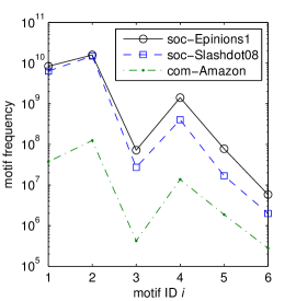
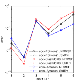
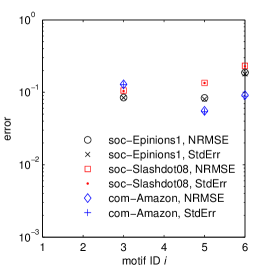
Figure 2: NRMSEs and StdErrs of the estimates of 4-node motif frequencies n1,,n6subscript𝑛1subscript𝑛6n_{1},\ldots,n_{6} given by MOSS-4 and MOSS-4Min, K=1,000𝐾1000K=1,000 and Kˇ=1,000ˇ𝐾1000\check{K}=1,000.

6 Data Evaluation

6.1 Datasets

We perform our experiments on the following publicly available datasets taken from the Stanford Network Analysis Platform (SNAP)111www.snap.stanford.edu, which are summarized in Table 3.

Table 3: Graph datasets used in our experiments. “edges" refers to the number of edges in the undirected graph generated by discarding edge labels. “max-degree" represents the maximum number of edges incident to a node in the undirected graph.
Graph nodes edges max-degree
soc-Epinions1 [24] 75,897 405,740 3,044
soc-Slashdot08 [18] 77,360 469,180 2,539
com-DBLP [32] 317,080 1,049,866 343
com-Amazon [32] 334,863 925,872 549
p2p-Gnutella08 [25] 6,301 20,777 97
ca-GrQc [17] 5,241 14,484 81
ca-CondMat [17] 23,133 93,439 279
ca-HepTh [17] 9,875 25,937 65

6.2 Error Metric

We study the normalized root mean square error (NRMSE) to measure the relative error of the motif frequency estimate n^isubscript^𝑛𝑖\hat{n}_{i} with respect to its true value nisubscript𝑛𝑖n_{i}, i=1,,6𝑖16i=1,\dots,6. NRMSE(n^i)NRMSEsubscript^𝑛𝑖\text{NRMSE}(\hat{n}_{i}) is defined as:

NRMSE(n^i)=MSE(n^i)ni,i=1,,6,formulae-sequenceNRMSEsubscript^𝑛𝑖MSEsubscript^𝑛𝑖subscript𝑛𝑖𝑖16\text{NRMSE}(\hat{n}_{i})=\frac{\sqrt{\text{MSE}(\hat{n}_{i})}}{n_{i}},\qquad i=1,\dots,6,

where MSE(n^i)MSEsubscript^𝑛𝑖\text{MSE}(\hat{n}_{i}) is defined as

MSE(n^i)=𝔼[(n^ini)2]=Var(n^i)+(𝔼[n^i]ni)2.MSEsubscript^𝑛𝑖𝔼delimited-[]superscriptsubscript^𝑛𝑖subscript𝑛𝑖2Varsubscript^𝑛𝑖superscript𝔼delimited-[]subscript^𝑛𝑖subscript𝑛𝑖2\text{MSE}(\hat{n}_{i})=\mathbb{E}[(\hat{n}_{i}-n_{i})^{2}]=\text{Var}(\hat{n}_{i})+\left(\mathbb{E}[\hat{n}_{i}]-n_{i}\right)^{2}.

Moreover, we define a standard error (in short, StdErr) of n^isubscript^𝑛𝑖\hat{n}_{i} as

StdErr(n^i)=Var(n^i)ni,i=1,,6.formulae-sequenceStdErrsubscript^𝑛𝑖Varsubscript^𝑛𝑖subscript𝑛𝑖𝑖16\text{StdErr}(\hat{n}_{i})=\frac{\sqrt{\text{Var}(\hat{n}_{i})}}{n_{i}},\qquad i=1,\dots,6.

We can see that MSE(n^i)MSEsubscript^𝑛𝑖\text{MSE}(\hat{n}_{i}) decomposes into a sum of the variance and bias of the estimator n^isubscript^𝑛𝑖\hat{n}_{i}, both quantities are important and need to be as small as possible to achieve good estimation performance. When n^isubscript^𝑛𝑖\hat{n}_{i} is an unbiased estimator of nisubscript𝑛𝑖n_{i}, then MSE(n^i)=Var(n^i)MSEsubscript^𝑛𝑖Varsubscript^𝑛𝑖\text{MSE}(\hat{n}_{i})=\text{Var}(\hat{n}_{i}) and thus NRMSE(n^i)NRMSEsubscript^𝑛𝑖\text{NRMSE}(\hat{n}_{i}) is equivalent to the normalized standard error of n^isubscript^𝑛𝑖\hat{n}_{i}, i.e., NRMSE(n^i)=Var(n^i)/ni=StdErr(n^i)NRMSEsubscript^𝑛𝑖Varsubscript^𝑛𝑖subscript𝑛𝑖StdErrsubscript^𝑛𝑖\text{NRMSE}(\hat{n}_{i})=\sqrt{\text{Var}(\hat{n}_{i})}/n_{i}=\text{StdErr}(\hat{n}_{i}). In our experiments, we average the estimates and calculate their NRMSEs over 1,000 runs. Similarly, we define NRMSE(nˇi)NRMSEsubscriptˇ𝑛𝑖\text{NRMSE}(\check{n}_{i}) and NRMSE(η^i)NRMSEsubscript^𝜂𝑖\text{NRMSE}(\hat{\eta}_{i}) for methods MOSS-4Min and MOSS-5. To validate the effective of our analytical error bounds, we also compute StdErrs of MOSS-4, MOSS-4Min, and MOSS-5 based on the derived closed formula of Var(n^i)Varsubscript^𝑛𝑖\text{Var}(\hat{n}_{i}), Var(nˇi)Varsubscriptˇ𝑛𝑖\text{Var}(\check{n}_{i}), and Var(η^i)Varsubscript^𝜂𝑖\text{Var}(\hat{\eta}_{i}).

Refer to caption
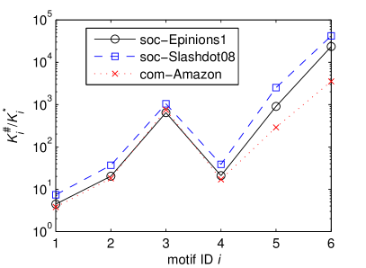
Figure 3: The values of Ki#/Kisubscriptsuperscript𝐾#𝑖subscriptsuperscript𝐾𝑖K^{\#}_{i}/K^{*}_{i}.
Refer to caption
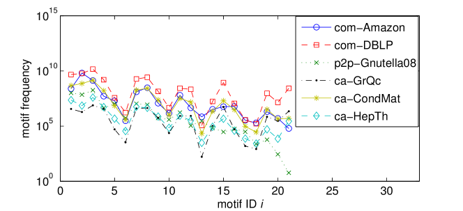
Figure 4: Real values of ηisubscript𝜂𝑖\eta_{i}, 1i211𝑖211\leq i\leq 21.

6.3 Estimating all 4-node motifs’ frequencies

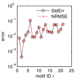
Figure 2(a) shows the real values of 4-node motif frequencies n1(4),,n6(4)superscriptsubscript𝑛14superscriptsubscript𝑛64n_{1}^{(4)},\ldots,n_{6}^{(4)} for graphs com-Epinions1, soc-Slashdot08, and com-Amazon, which have 2.58×10102.58superscript10102.58\times 10^{10}, 2.17×10102.17superscript10102.17\times 10^{10}, and 1.78×1081.78superscript1081.78\times 10^{8} 4-node CISes respectively. We can see that the motif frequencies of M3(4)superscriptsubscript𝑀34M_{3}^{(4)}, M5(4)superscriptsubscript𝑀54M_{5}^{(4)}, and M6(4)superscriptsubscript𝑀64M_{6}^{(4)} are several orders of magnitude smaller than that of the other motifs. Fig 2(b) shows the NRMSEs and StdErrs of n^1(4),,n^6(4)superscriptsubscript^𝑛14superscriptsubscript^𝑛64\hat{n}_{1}^{(4)},\ldots,\hat{n}_{6}^{(4)}, the estimates of 4-node undirected motifs’ frequencies given by MOSS-4, where we set K=1,000𝐾1000K=1,000. we can see that motifs with high frequencies exhibit larger NRMSEs and StdErrs than motifs with low frequencies. Moreover, we observe that the StdErr of n^i(4)superscriptsubscript^𝑛𝑖4\hat{n}_{i}^{(4)} almost equals to the NRMSE of n^i(4)superscriptsubscript^𝑛𝑖4\hat{n}_{i}^{(4)}, which is consistent to our analysis above. Our derived error formulas indicate that the StdErr of n^i(4)superscriptsubscript^𝑛𝑖4\hat{n}_{i}^{(4)} decreases linearly with the sampling budget K𝐾\sqrt{K}, which helps us to estimate the computational time required to guarantee certain accuracy for the estimate in advance. Fig 2(c) shows the NRMSEs and StdErrs of nˇ3(4)superscriptsubscriptˇ𝑛34\check{n}_{3}^{(4)}, nˇ5(4)superscriptsubscriptˇ𝑛54\check{n}_{5}^{(4)}, and nˇ6(4)superscriptsubscriptˇ𝑛64\check{n}_{6}^{(4)} given by MOSS-4MIN, where we set Kˇ=1,000ˇ𝐾1000\check{K}=1,000. Similarly, we see that the StdErr of n^i(4)superscriptsubscript^𝑛𝑖4\hat{n}_{i}^{(4)} almost equals to the NRMSE of n^i(4)superscriptsubscript^𝑛𝑖4\hat{n}_{i}^{(4)}, i=3,5,6𝑖356i=3,5,6. We compute NRMSE(n^i)NRMSE(nˇi)NRMSEsubscript^𝑛𝑖NRMSEsubscriptˇ𝑛𝑖\frac{\text{NRMSE}(\hat{n}_{i})}{\text{NRMSE}(\check{n}_{i})} to evaluate the performance of MOSS-4Min in comparison with MOSS-4. NRMSE(n^i)NRMSE(nˇi)NRMSEsubscript^𝑛𝑖NRMSEsubscriptˇ𝑛𝑖\frac{\text{NRMSE}(\hat{n}_{i})}{\text{NRMSE}(\check{n}_{i})} of soc-Slashdot08 is 2.4, 1.9, and 2.3 for i=3𝑖3i=3, i=5𝑖5i=5, and i=6𝑖6i=6 respectively. NRMSE(n^i)NRMSE(nˇi)NRMSEsubscript^𝑛𝑖NRMSEsubscriptˇ𝑛𝑖\frac{\text{NRMSE}(\hat{n}_{i})}{\text{NRMSE}(\check{n}_{i})} of com-Epinions1 is 2.5, 2.0, and 2.4 for i=3𝑖3i=3, i=5𝑖5i=5, and i=6𝑖6i=6 respectively. NRMSE(n^i)NRMSE(nˇi)NRMSEsubscript^𝑛𝑖NRMSEsubscriptˇ𝑛𝑖\frac{\text{NRMSE}(\hat{n}_{i})}{\text{NRMSE}(\check{n}_{i})} of com-Amazon is 1.7, 1.5, and 1.8 for i=3𝑖3i=3, i=5𝑖5i=5, and i=6𝑖6i=6 respectively. NRMSE(n^i)NRMSE(nˇi)NRMSEsubscript^𝑛𝑖NRMSEsubscriptˇ𝑛𝑖\frac{\text{NRMSE}(\hat{n}_{i})}{\text{NRMSE}(\check{n}_{i})} of ca-GrQc is 1.1, 0.9, and 1.8 for i=3𝑖3i=3, i=5𝑖5i=5, and i=6𝑖6i=6 respectively. We can see that MOSS-4Min exhibits a slightly improvement for ca-GrQc, so it is consistent to the analysis in Section 4.5. To guarantee P(|n^ini|>εni)<δ𝑃subscript^𝑛𝑖subscript𝑛𝑖𝜀subscript𝑛𝑖𝛿P(|\hat{n}_{i}-n_{i}|>\varepsilon n_{i})<\delta, i=1,,6𝑖16i=1,\ldots,6, we let Kisuperscriptsubscript𝐾𝑖K_{i}^{*} and Ki#superscriptsubscript𝐾𝑖#K_{i}^{\#} denote the smallest sampling budgets that are determined by our method and the method in [11] respectively. Fig. 3 shows the values of Ki#/Kisubscriptsuperscript𝐾#𝑖subscriptsuperscript𝐾𝑖K^{\#}_{i}/K^{*}_{i}, where ε=0.1𝜀0.1\varepsilon=0.1 and δ=0.01𝛿0.01\delta=0.01. We can see that the sampling budgets given by the method in [11] are several orders of magnitude larger than our method. It indicates that the method in [11] does not bound the estimation error tightly and so it significantly over-estimates the sampling budget required to achieve a certain accuracy.
Refer to caption
(a) com-Amazon
Refer to caption
(b) soc-DBLP
Refer to caption
(c) p2p-Gnutella08
Refer to caption
(d) ca-GrQc
Refer to caption
(e) ca-CondMat
Refer to caption
(f) ca-HepTh
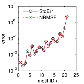
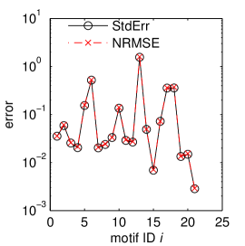
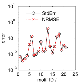
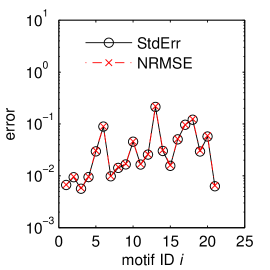
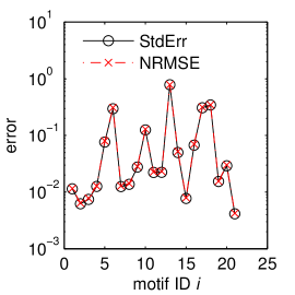
Figure 5: Real values, StdErrs, and NRMSEs of η^i(5)superscriptsubscript^𝜂𝑖5\hat{\eta}_{i}^{(5)}, i.e., the motif frequency estimates of Mi(5)superscriptsubscript𝑀𝑖5M_{i}^{(5)}, 1i211𝑖211\leq i\leq 21, where K1=50,000subscript𝐾150000K_{1}=50,000 and K2=50,000subscript𝐾250000K_{2}=50,000.

6.4 Estimating all 5-node motifs’ frequencies

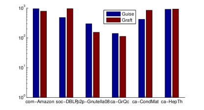
Figure 4 shows the real values of η1,,η21subscript𝜂1subscript𝜂21\eta_{1},\ldots,\eta_{21} for graphs com-Amazon, com-DBLP, p2p-Gnutella08, ca-GrQc, ca-CondMat, and ca-HepTh, which have 8.50×1098.50superscript1098.50\times 10^{9}, 3.34×10103.34superscript10103.34\times 10^{10}, 3.92×1083.92superscript1083.92\times 10^{8}, 3.64×1073.64superscript1073.64\times 10^{7}, 3.32×1093.32superscript1093.32\times 10^{9}, and 8.73×1078.73superscript1078.73\times 10^{7} 5-node CISes respectively. Fig 5 shows the NRMSEs and StdErrs of η^1(5),,η^21(5)superscriptsubscript^𝜂15superscriptsubscript^𝜂215\hat{\eta}_{1}^{(5)},\ldots,\hat{\eta}_{21}^{(5)}, where we set K1=50,000subscript𝐾150000K_{1}=50,000 and K2=50,000subscript𝐾250000K_{2}=50,000. We can see that the StdErrs are very close to the NRMSEs. It indicates that the derived StdErrs can be accurately used to evaluate the error of our estimates given by MOSS-5. To the best of our knowledge, MOSS-5 is the first to provide a simple and accurate formula for analyzing estimation errors of 5-node motif frequencies. The results show that the NRMSEs of all 5-node motifs are smaller than 0.1 for com-Amazon, which is larger than the other graphs studied in this paper. For the other graphs, most 5-node motifs’ NRMSEs are smaller than 0.1. The NRMSE of η^21(5)superscriptsubscript^𝜂215\hat{\eta}_{21}^{(5)} is larger than 1 for p2p-Gnutella08, and the NRMSE of η^21(5)superscriptsubscript^𝜂215\hat{\eta}_{21}^{(5)} is larger than 1 for ca-GrQc. We observe that p2p-Gnutella08 has only several CISes isomorphic to M21(5)superscriptsubscript𝑀215M_{21}^{(5)}, and p2p-Gnutella08 has no more than 200 CISes isomorphic to M13(5)superscriptsubscript𝑀135M_{13}^{(5)}. It is very challenging to observe and count these rare motifs for sampling based methods. Most previous work focuses on estimating 5-node motif concentrations, which is defines as ωi=ηij=121ηjsubscript𝜔𝑖subscript𝜂𝑖superscriptsubscript𝑗121subscript𝜂𝑗\omega_{i}=\frac{\eta_{i}}{\sum_{j=1}^{21}\eta_{j}}, i=1,,21𝑖121i=1,\ldots,21. We run MOSS-5, state-of-the-arts methods Guise [4] and Graft [23] over all above graphs and increase their sampling budgets until the estimation errors of motif concentrations are within 10%. Fig. 6 shows the runtimes of Graft and Guise normalized with respect to the runtimes of MOSS-5. We can see that our method MOSS-5 is 2 to 3 orders of magnitude faster than Graft and Guise.
Refer to caption
Figure 6: Runtimes of the-state-of-art methods normalized with respect to runtimes of MOSS-5 for estimating 5-node motif concentrations.

7 Related Work

In this paper, we study the problem of computing 4- and 5-node motifs’ frequencies for a single large graph, which is much different from the problem of computing the number of subgraph patterns appearing in a large set of graphs studied in [7]. Recently, a lot of efforts has been devoted to design sampling methods for computing a large graph’s motif concentrations [14, 31, 21, 4, 23, 29]. However, these methods fail to compute motif frequencies, which is more fundamental than motif concentrations. Alon et al. [3] propose the color-coding method to reduce the computational cost of counting subgraphs. Color coding reduces the computations by coloring nodes randomly and enumerating only colorful CISes (i.e., CISes that are consisted of nodes with distinct colors), but [12] reaveals that the color-coding method is not scalable and is hindered by the sheer number of colorful CISes. [27, 22, 10, 1] develop sampling methods to estimate the number of triangles of static and dynamic graphs. Jha et al. [11] develop sampling methods to estimate 4-node undirected motifs’ frequencies. However their methods are edge centric methods, which cannot be easily applied to current vertex centric graph computing systems such as GraphLab [19] and GraphChi [16]. Moreover, their methods fail to sample and count 5-node motifs.

8 Conclusions

We develop computationally efficient sampling methods MOSS-4 and MOSS-5 to estimate the frequencies of all 4- and 5-node motifs. Compared MOSS-4, MOSS-4Min is better to characterize rare motifs. All these methods provide unbiased estimators of motif frequencies, and we derive simple and exact formulas for the variances of the estimators. Meanwhile, we conduct experiments on a variety of publicly available datasets, and experimental results show that our methods significantly outperform state-of-the-art methods.

Acknowledgment

This work was supported in part by the National Natural Science Foundation of China (61103240, 61103241, 61221063, 61221063, 91118005, U1301254), the 111 International Collaboration Program of China, 863 High Tech Development Plan (2012AA011003), the Prospective Research Project on Future Networks of Jiangsu Future Networks Innovation Institute, and the Application Foundation Research Program of SuZhou (SYG201311).

Appendix

Proof of Theorem 2

As shown in Fig. 7, we find that there exist two ways to sample a subgraph isomorphic to motif M1(4)superscriptsubscript𝑀14M_{1}^{(4)} by MOSS-4. Each one happens with probability πv×σu(v)×1dv1×1du1=1Γsubscript𝜋𝑣superscriptsubscript𝜎𝑢𝑣1subscript𝑑𝑣11subscript𝑑𝑢11Γ\pi_{v}\times\sigma_{u}^{(v)}\times\frac{1}{d_{v}-1}\times\frac{1}{d_{u}-1}=\frac{1}{\Gamma}. For a 4-node CIS s𝑠s isomorphic to motif Mi(4)superscriptsubscript𝑀𝑖4M_{i}^{(4)}, s𝑠s has φi(1)superscriptsubscript𝜑𝑖1\varphi_{i}^{(1)} subgraphs isomorphic to motif M1(4)superscriptsubscript𝑀14M_{1}^{(4)}, 1i61𝑖61\leq i\leq 6. Thus, there exist 2φi(1)2superscriptsubscript𝜑𝑖12\varphi_{i}^{(1)} ways to sample s𝑠s by MOSS-4, and the probability of MOSS-4 sampling s𝑠s is 2φi(1)Γ2superscriptsubscript𝜑𝑖1Γ\frac{2\varphi_{i}^{(1)}}{\Gamma}.

Refer to caption
Figure 7: The ways of MOSS-4 sampling a subgraph s𝑠s isomorphic to motif M1(4)superscriptsubscript𝑀14M_{1}^{(4)}, where v𝑣v, u𝑢u, w𝑤w, and r𝑟r are the variables in Algorithm 1, i.e., the nodes sampled at the 1-st, 2-nd, 3-rd, and 4-th steps respectively.

Proof of Theorem 3

For i{1,3,4,5,6}𝑖13456i\in\{1,3,4,5,6\} and 1kK1𝑘𝐾1\leq k\leq K, we have

P(M(4)(sk)=i)=sC(4)P(sk=s)𝟏(M(4)(s)=i)=pini.𝑃superscript𝑀4subscript𝑠𝑘𝑖subscript𝑠superscript𝐶4𝑃subscript𝑠𝑘𝑠1superscript𝑀4𝑠𝑖subscript𝑝𝑖subscript𝑛𝑖P(M^{(4)}(s_{k})=i)=\sum_{s\in C^{(4)}}P(s_{k}=s)\mathbf{1}(M^{(4)}(s)=i)=p_{i}n_{i}.

s1,,sKsubscript𝑠1subscript𝑠𝐾s_{1},\ldots,s_{K} are sampled independently, so the random variable misubscript𝑚𝑖m_{i} follows the binomial distribution with parameters K𝐾K and pinisubscript𝑝𝑖subscript𝑛𝑖p_{i}n_{i}. Formally, we have

P(mi=x)=(Kx)(pini)x(1pini)Kx,x=0,1,,K.formulae-sequence𝑃subscript𝑚𝑖𝑥binomial𝐾𝑥superscriptsubscript𝑝𝑖subscript𝑛𝑖𝑥superscript1subscript𝑝𝑖subscript𝑛𝑖𝐾𝑥𝑥01𝐾P(m_{i}=x)=\binom{K}{x}(p_{i}n_{i})^{x}(1-p_{i}n_{i})^{K-x},\quad x=0,1,\ldots,K.

Then, the expectation and variance of misubscript𝑚𝑖m_{i} are

𝔼(mi)=Kpini,𝔼subscript𝑚𝑖𝐾subscript𝑝𝑖subscript𝑛𝑖\mathbb{E}(m_{i})=Kp_{i}n_{i},

and

Var(mi)=Kpini(1pini).Varsubscript𝑚𝑖𝐾subscript𝑝𝑖subscript𝑛𝑖1subscript𝑝𝑖subscript𝑛𝑖\text{Var}(m_{i})=Kp_{i}n_{i}(1-p_{i}n_{i}).

Therefore, the expectation and variance of n^isubscript^𝑛𝑖\hat{n}_{i} are computed as

𝔼(n^i)=𝔼(miKpi)=𝔼(mi)Kpi=ni,𝔼subscript^𝑛𝑖𝔼subscript𝑚𝑖𝐾subscript𝑝𝑖𝔼subscript𝑚𝑖𝐾subscript𝑝𝑖subscript𝑛𝑖\mathbb{E}(\hat{n}_{i})=\mathbb{E}\left(\frac{m_{i}}{Kp_{i}}\right)=\frac{\mathbb{E}(m_{i})}{Kp_{i}}=n_{i}, (8)

and

Var(n^i)=Var(miKpi)=Var(mi)K2pi2=niK(1pini).Varsubscript^𝑛𝑖Varsubscript𝑚𝑖𝐾subscript𝑝𝑖Varsubscript𝑚𝑖superscript𝐾2superscriptsubscript𝑝𝑖2subscript𝑛𝑖𝐾1subscript𝑝𝑖subscript𝑛𝑖\text{Var}(\hat{n}_{i})=\text{Var}\left(\frac{m_{i}}{Kp_{i}}\right)=\frac{\text{Var}(m_{i})}{K^{2}p_{i}^{2}}=\frac{n_{i}}{K}\left(\frac{1}{p_{i}}-n_{i}\right). (9)

From (8), we compute the expectation of n^2subscript^𝑛2\hat{n}_{2} as

𝔼(n^2)=𝔼(Λ3n^42n^54n^6)=Λ3𝔼(n^4)2𝔼(n^5)4𝔼(n^6)=Λ3n42n54n6=n2.𝔼subscript^𝑛2𝔼subscriptΛ3subscript^𝑛42subscript^𝑛54subscript^𝑛6subscriptΛ3𝔼subscript^𝑛42𝔼subscript^𝑛54𝔼subscript^𝑛6subscriptΛ3subscript𝑛42subscript𝑛54subscript𝑛6subscript𝑛2\begin{split}\mathbb{E}(\hat{n}_{2})&=\mathbb{E}(\Lambda_{3}-\hat{n}_{4}-2\hat{n}_{5}-4\hat{n}_{6})\\ &=\Lambda_{3}-\mathbb{E}(\hat{n}_{4})-2\mathbb{E}(\hat{n}_{5})-4\mathbb{E}(\hat{n}_{6})\\ &=\Lambda_{3}-n_{4}-2n_{5}-4n_{6}\\ &=n_{2}.\end{split}

The last equation holds because of (2). To derive the variance of n^2subscript^𝑛2\hat{n}_{2}, we first compute the covariance of n^isubscript^𝑛𝑖\hat{n}_{i} and n^jsubscript^𝑛𝑗\hat{n}_{j}, where ij𝑖𝑗i\neq j and i,j{1,3,4,5,6}𝑖𝑗13456i,j\in\{1,3,4,5,6\}. That is,

Cov(n^i,n^j)Covsubscript^𝑛𝑖subscript^𝑛𝑗\displaystyle\text{Cov}(\hat{n}_{i},\hat{n}_{j}) (10)
=\displaystyle= Cov(miKpi,mjKpj)Covsubscript𝑚𝑖𝐾subscript𝑝𝑖subscript𝑚𝑗𝐾subscript𝑝𝑗\displaystyle\text{Cov}\left(\frac{m_{i}}{Kp_{i}},\frac{m_{j}}{Kp_{j}}\right)
=\displaystyle= Cov(k=1K𝟏(M(4)(sk)=i),l=1K𝟏(M(4)(sl)=j))K2pipjCovsuperscriptsubscript𝑘1𝐾1superscript𝑀4subscript𝑠𝑘𝑖superscriptsubscript𝑙1𝐾1superscript𝑀4subscript𝑠𝑙𝑗superscript𝐾2subscript𝑝𝑖subscript𝑝𝑗\displaystyle\frac{\text{Cov}(\sum_{k=1}^{K}\mathbf{1}(M^{(4)}(s_{k})=i),\sum_{l=1}^{K}\mathbf{1}(M^{(4)}(s_{l})=j))}{K^{2}p_{i}p_{j}}
=\displaystyle= k=1Kl=1KCov(𝟏(M(4)(sk)=i),𝟏(M(4)(sl)=j))K2pipjsuperscriptsubscript𝑘1𝐾superscriptsubscript𝑙1𝐾Cov1superscript𝑀4subscript𝑠𝑘𝑖1superscript𝑀4subscript𝑠𝑙𝑗superscript𝐾2subscript𝑝𝑖subscript𝑝𝑗\displaystyle\frac{\sum_{k=1}^{K}\sum_{l=1}^{K}\text{Cov}(\mathbf{1}(M^{(4)}(s_{k})=i),\mathbf{1}(M^{(4)}(s_{l})=j))}{K^{2}p_{i}p_{j}}
=\displaystyle= k=1KCov(𝟏(M(4)(sk)=i),𝟏(M(4)(sk)=j))K2pipjsuperscriptsubscript𝑘1𝐾Cov1superscript𝑀4subscript𝑠𝑘𝑖1superscript𝑀4subscript𝑠𝑘𝑗superscript𝐾2subscript𝑝𝑖subscript𝑝𝑗\displaystyle\frac{\sum_{k=1}^{K}\text{Cov}(\mathbf{1}(M^{(4)}(s_{k})=i),\mathbf{1}(M^{(4)}(s_{k})=j))}{K^{2}p_{i}p_{j}}
=\displaystyle= ninjK.subscript𝑛𝑖subscript𝑛𝑗𝐾\displaystyle-\frac{n_{i}n_{j}}{K}.

In the derivation above, we use

Cov(𝟏(M(4)(sk)=i),𝟏(M(4)(sk)=j))=E(𝟏(M(4)(sk)=i)𝟏(M(4)(sk)=j))E(𝟏(M(4)(sk)=i))E(𝟏(M(4)(sk)=j))=0pinipjnj=pipjninj,Cov1superscript𝑀4subscript𝑠𝑘𝑖1superscript𝑀4subscript𝑠𝑘𝑗E1superscript𝑀4subscript𝑠𝑘𝑖1superscript𝑀4subscript𝑠𝑘𝑗E1superscript𝑀4subscript𝑠𝑘𝑖E1superscript𝑀4subscript𝑠𝑘𝑗0subscript𝑝𝑖subscript𝑛𝑖subscript𝑝𝑗subscript𝑛𝑗subscript𝑝𝑖subscript𝑝𝑗subscript𝑛𝑖subscript𝑛𝑗\begin{split}&\text{Cov}(\mathbf{1}(M^{(4)}(s_{k})=i),\mathbf{1}(M^{(4)}(s_{k})=j))\\ &=\text{E}(\mathbf{1}(M^{(4)}(s_{k})=i)\mathbf{1}(M^{(4)}(s_{k})=j))\\ &\quad-\text{E}(\mathbf{1}(M^{(4)}(s_{k})=i))\text{E}(\mathbf{1}(M^{(4)}(s_{k})=j))\\ &=0-p_{i}n_{i}p_{j}n_{j}\\ &=-p_{i}p_{j}n_{i}n_{j},\end{split}

and Cov(𝟏(M(4)(sk)=i),𝟏(M(4)(sl)=j))=0Cov1superscript𝑀4subscript𝑠𝑘𝑖1superscript𝑀4subscript𝑠𝑙𝑗0\text{Cov}(\mathbf{1}(M^{(4)}(s_{k})=i),\mathbf{1}(M^{(4)}(s_{l})=j))=0 when kl𝑘𝑙k\neq l. Finally, we compute the variance of n^2subscript^𝑛2\hat{n}_{2} as

Var(n^2)=Var(Λ3n^42n^54n^6)=Var(n^4+2n^5+4n^6)=Var(n^4)+4Var(n^5)+16Var(n^6)+4Cov(n^4n^5)+8Cov(n^4n^6)+16Cov(n^5n^6).Varsubscript^𝑛2VarsubscriptΛ3subscript^𝑛42subscript^𝑛54subscript^𝑛6Varsubscript^𝑛42subscript^𝑛54subscript^𝑛6Varsubscript^𝑛44Varsubscript^𝑛516Varsubscript^𝑛64Covsubscript^𝑛4subscript^𝑛58Covsubscript^𝑛4subscript^𝑛616Covsubscript^𝑛5subscript^𝑛6\begin{split}\text{Var}(\hat{n}_{2})&=\text{Var}(\Lambda_{3}-\hat{n}_{4}-2\hat{n}_{5}-4\hat{n}_{6})\\ &=\text{Var}(\hat{n}_{4}+2\hat{n}_{5}+4\hat{n}_{6})\\ &=\text{Var}(\hat{n}_{4})+4\text{Var}(\hat{n}_{5})+16\text{Var}(\hat{n}_{6})\\ &\quad+4\text{Cov}(\hat{n}_{4}\hat{n}_{5})+8\text{Cov}(\hat{n}_{4}\hat{n}_{6})+16\text{Cov}(\hat{n}_{5}\hat{n}_{6}).\end{split}

Using (9) and (10), then we have

Var(n^2)=1K(n4p4+4n5p5+16n6p6(n4+2n5+4n6)2).Varsubscript^𝑛21𝐾subscript𝑛4subscript𝑝44subscript𝑛5subscript𝑝516subscript𝑛6subscript𝑝6superscriptsubscript𝑛42subscript𝑛54subscript𝑛62\text{Var}(\hat{n}_{2})=\frac{1}{K}\left(\frac{n_{4}}{p_{4}}+\frac{4n_{5}}{p_{5}}+\frac{16n_{6}}{p_{6}}-(n_{4}+2n_{5}+4n_{6})^{2}\right).

Proof of Theorem 4

Let φˇ(1)(s)superscriptˇ𝜑1𝑠\check{\varphi}^{(1)}(s) denote the number of ways to sample a 4-node CIS s𝑠s by MOSS-4Min. Then, we have pˇ(s)=φˇ(1)(s)×πˇv×σˇu(v)×1dv,u×1du,v=φˇ(1)(s)Γˇ1ˇ𝑝𝑠superscriptˇ𝜑1𝑠subscriptˇ𝜋𝑣superscriptsubscriptˇ𝜎𝑢𝑣1subscript𝑑𝑣𝑢1subscript𝑑𝑢𝑣superscriptˇ𝜑1𝑠superscriptˇΓ1\check{p}(s)=\check{\varphi}^{(1)}(s)\times\check{\pi}_{v}\times\check{\sigma}_{u}^{(v)}\times\frac{1}{d_{v,u}}\times\frac{1}{d_{u,v}}=\check{\varphi}^{(1)}(s)\check{\Gamma}^{-1}. We compute φˇ(1)(s1)=2superscriptˇ𝜑1subscript𝑠12\check{\varphi}^{(1)}(s_{1})=2, φˇ(1)(s2)=2superscriptˇ𝜑1subscript𝑠22\check{\varphi}^{(1)}(s_{2})=2, and φˇ(1)(s3)=6superscriptˇ𝜑1subscript𝑠36\check{\varphi}^{(1)}(s_{3})=6 for cases s1C3(4)subscript𝑠1superscriptsubscript𝐶34s_{1}\in C_{3}^{(4)}, s2C5(4)subscript𝑠2superscriptsubscript𝐶54s_{2}\in C_{5}^{(4)}, and s3C6(4)subscript𝑠3superscriptsubscript𝐶64s_{3}\in C_{6}^{(4)} respectively.

Proof of Theorem 6

As shown in Fig. 8, we find that there exist two ways to sample a subgraph isomorphic to motif M3(5)superscriptsubscript𝑀35M_{3}^{(5)} by T-5. Each one happens with probability ρv(1)×σu(v)×1dv1×1dv2×1du1=1Γ(1)superscriptsubscript𝜌𝑣1superscriptsubscript𝜎𝑢𝑣1subscript𝑑𝑣11subscript𝑑𝑣21subscript𝑑𝑢11superscriptΓ1\rho_{v}^{(1)}\times\sigma_{u}^{(v)}\times\frac{1}{d_{v}-1}\times\frac{1}{d_{v}-2}\times\frac{1}{d_{u}-1}=\frac{1}{\Gamma^{(1)}}. For a 5-node CIS s𝑠s isomorphic to motif Mi(5)superscriptsubscript𝑀𝑖5M_{i}^{(5)}, s𝑠s has ϕi(1)superscriptsubscriptitalic-ϕ𝑖1\phi_{i}^{(1)} subgraphs isomorphic to motif M3(5)superscriptsubscript𝑀35M_{3}^{(5)}, 1i211𝑖211\leq i\leq 21. Therefore, the probability of sampling s𝑠s is 2ϕi(1)Γ(1)2superscriptsubscriptitalic-ϕ𝑖1superscriptΓ1\frac{2\phi_{i}^{(1)}}{\Gamma^{(1)}}.

Refer to caption
Figure 8: The ways of T-5 sampling a subgraph s𝑠s isomorphic to motif M3(5)superscriptsubscript𝑀35M_{3}^{(5)}, where v𝑣v, u𝑢u, w𝑤w, r𝑟r, and t𝑡t are the variables in Algorithm 3, i.e., the nodes sampled at the 1-st, 2-nd, 3-rd, 4-th, and 5-th steps respectively.

Proof of Theorem 7

For iΩ1𝑖subscriptΩ1i\in\Omega_{1} and 1kK11𝑘subscript𝐾11\leq k\leq K_{1}, we have

P(M(5)(sk(1))=i)=sC(5)P(sk(1)=s)𝟏(M(5)(sk(1))=i)=pi(1)ηi.𝑃superscript𝑀5superscriptsubscript𝑠𝑘1𝑖subscript𝑠superscript𝐶5𝑃superscriptsubscript𝑠𝑘1𝑠1superscript𝑀5superscriptsubscript𝑠𝑘1𝑖superscriptsubscript𝑝𝑖1subscript𝜂𝑖\begin{split}P(M^{(5)}(s_{k}^{(1)})=i)&=\sum_{s\in C^{(5)}}P(s_{k}^{(1)}=s)\mathbf{1}(M^{(5)}(s_{k}^{(1)})=i)\\ &=p_{i}^{(1)}\eta_{i}.\end{split}

Since s1(1),,sK1(1)superscriptsubscript𝑠11superscriptsubscript𝑠subscript𝐾11s_{1}^{(1)},\ldots,s_{K_{1}}^{(1)} are sampled independently, the random variable mi(1)superscriptsubscript𝑚𝑖1m_{i}^{(1)} follows the binomial distribution with parameters K1subscript𝐾1K_{1} and pi(1)ηisuperscriptsubscript𝑝𝑖1subscript𝜂𝑖p_{i}^{(1)}\eta_{i}. Then, the expectation and variance of mi(1)superscriptsubscript𝑚𝑖1m_{i}^{(1)} are

𝔼(mi(1))=K1pi(1)ηi,𝔼superscriptsubscript𝑚𝑖1subscript𝐾1superscriptsubscript𝑝𝑖1subscript𝜂𝑖\mathbb{E}(m_{i}^{(1)})=K_{1}p_{i}^{(1)}\eta_{i},

and

Var(mi(1))=K1pi(1)ηi(1pi(1)ηi).Varsuperscriptsubscript𝑚𝑖1subscript𝐾1superscriptsubscript𝑝𝑖1subscript𝜂𝑖1superscriptsubscript𝑝𝑖1subscript𝜂𝑖\text{Var}(m_{i}^{(1)})=K_{1}p_{i}^{(1)}\eta_{i}(1-p_{i}^{(1)}\eta_{i}). (11)

Therefore, the expectation and variance of η^i(1)superscriptsubscript^𝜂𝑖1\hat{\eta}_{i}^{(1)} are computed as

𝔼(η^i(1))=𝔼(mi(1)K1pi(1))=𝔼(mi(1))K1pi(1)=ηi,𝔼superscriptsubscript^𝜂𝑖1𝔼superscriptsubscript𝑚𝑖1subscript𝐾1superscriptsubscript𝑝𝑖1𝔼superscriptsubscript𝑚𝑖1subscript𝐾1superscriptsubscript𝑝𝑖1subscript𝜂𝑖\mathbb{E}(\hat{\eta}_{i}^{(1)})=\mathbb{E}\left(\frac{m_{i}^{(1)}}{K_{1}p_{i}^{(1)}}\right)=\frac{\mathbb{E}(m_{i}^{(1)})}{K_{1}p_{i}^{(1)}}=\eta_{i},

and

Var(η^i)=Var(mi(1)K1pi(1))=ηiK1(1pi(1)ηi).Varsubscript^𝜂𝑖Varsuperscriptsubscript𝑚𝑖1subscript𝐾1superscriptsubscript𝑝𝑖1subscript𝜂𝑖subscript𝐾11superscriptsubscript𝑝𝑖1subscript𝜂𝑖\text{Var}(\hat{\eta}_{i})=\text{Var}\left(\frac{m_{i}^{(1)}}{K_{1}p_{i}^{(1)}}\right)=\frac{\eta_{i}}{K_{1}}\left(\frac{1}{p_{i}^{(1)}}-\eta_{i}\right).

For ij𝑖𝑗i\neq j and i,jΩ1𝑖𝑗subscriptΩ1i,j\in\Omega_{1}, the covariance of η^i(1)superscriptsubscript^𝜂𝑖1\hat{\eta}_{i}^{(1)} and η^j(1)superscriptsubscript^𝜂𝑗1\hat{\eta}_{j}^{(1)} is

Cov(η^i(1),η^j(1))Covsuperscriptsubscript^𝜂𝑖1superscriptsubscript^𝜂𝑗1\displaystyle\text{Cov}(\hat{\eta}_{i}^{(1)},\hat{\eta}_{j}^{(1)})
=\displaystyle= Cov(mi(1)K1pi(1),mj(1)K1pj(1))Covsuperscriptsubscript𝑚𝑖1subscript𝐾1superscriptsubscript𝑝𝑖1superscriptsubscript𝑚𝑗1subscript𝐾1superscriptsubscript𝑝𝑗1\displaystyle\text{Cov}\left(\frac{m_{i}^{(1)}}{K_{1}p_{i}^{(1)}},\frac{m_{j}^{(1)}}{K_{1}p_{j}^{(1)}}\right)
=\displaystyle= Cov(k=1K1𝟏(M(5)(sk(1))=i),l=1K1𝟏(M(5)(sl(1))=j))K12pi(1)pj(1)Covsuperscriptsubscript𝑘1subscript𝐾11superscript𝑀5superscriptsubscript𝑠𝑘1𝑖superscriptsubscript𝑙1subscript𝐾11superscript𝑀5superscriptsubscript𝑠𝑙1𝑗superscriptsubscript𝐾12superscriptsubscript𝑝𝑖1superscriptsubscript𝑝𝑗1\displaystyle\frac{\text{Cov}(\sum_{k=1}^{K_{1}}\mathbf{1}(M^{(5)}(s_{k}^{(1)})=i),\sum_{l=1}^{K_{1}}\mathbf{1}(M^{(5)}(s_{l}^{(1)})=j))}{K_{1}^{2}p_{i}^{(1)}p_{j}^{(1)}}
=\displaystyle= k=1K1l=1K1Cov(𝟏(M(5)(sk(1))=i),𝟏(M(5)(sl(1))=j))K12pi(1)pj(1)superscriptsubscript𝑘1subscript𝐾1superscriptsubscript𝑙1subscript𝐾1Cov1superscript𝑀5superscriptsubscript𝑠𝑘1𝑖1superscript𝑀5superscriptsubscript𝑠𝑙1𝑗superscriptsubscript𝐾12superscriptsubscript𝑝𝑖1superscriptsubscript𝑝𝑗1\displaystyle\frac{\sum_{k=1}^{K_{1}}\sum_{l=1}^{K_{1}}\text{Cov}(\mathbf{1}(M^{(5)}(s_{k}^{(1)})=i),\mathbf{1}(M^{(5)}(s_{l}^{(1)})=j))}{K_{1}^{2}p_{i}^{(1)}p_{j}^{(1)}}
=\displaystyle= k=1K1Cov(𝟏(M(5)(sk(1))=i),𝟏(M(5)(sk(1))=j))K12pi(1)pj(1)superscriptsubscript𝑘1subscript𝐾1Cov1superscript𝑀5superscriptsubscript𝑠𝑘1𝑖1superscript𝑀5superscriptsubscript𝑠𝑘1𝑗superscriptsubscript𝐾12superscriptsubscript𝑝𝑖1superscriptsubscript𝑝𝑗1\displaystyle\frac{\sum_{k=1}^{K_{1}}\text{Cov}(\mathbf{1}(M^{(5)}(s_{k}^{(1)})=i),\mathbf{1}(M^{(5)}(s_{k}^{(1)})=j))}{K_{1}^{2}p_{i}^{(1)}p_{j}^{(1)}}
=\displaystyle= ηiηjK1.subscript𝜂𝑖subscript𝜂𝑗subscript𝐾1\displaystyle-\frac{\eta_{i}\eta_{j}}{K_{1}}.

In the derivation above, we use

Cov(𝟏(M(5)(sk(1))=i),𝟏(M(5)(sl(1))=j))=0,kl,formulae-sequenceCov1superscript𝑀5superscriptsubscript𝑠𝑘1𝑖1superscript𝑀5superscriptsubscript𝑠𝑙1𝑗0𝑘𝑙\text{Cov}(\mathbf{1}(M^{(5)}(s_{k}^{(1)})=i),\mathbf{1}(M^{(5)}(s_{l}^{(1)})=j))=0,\quad k\neq l,

and

Cov(𝟏(M(5)(sk(1))=i),𝟏(M(5)(sk(1))=j))=E(𝟏(M(5)(sk(1))=i)𝟏(M(5)(sk(1))=j))E(𝟏(M(5)(sk(1))=i))E(𝟏(M(5)(sk(1))=j))=0pi(1)ηipj(1)ηj=pi(1)pj(1)ηiηj.Cov1superscript𝑀5superscriptsubscript𝑠𝑘1𝑖1superscript𝑀5superscriptsubscript𝑠𝑘1𝑗E1superscript𝑀5superscriptsubscript𝑠𝑘1𝑖1superscript𝑀5superscriptsubscript𝑠𝑘1𝑗E1superscript𝑀5superscriptsubscript𝑠𝑘1𝑖E1superscript𝑀5superscriptsubscript𝑠𝑘1𝑗0superscriptsubscript𝑝𝑖1subscript𝜂𝑖subscriptsuperscript𝑝1𝑗subscript𝜂𝑗superscriptsubscript𝑝𝑖1superscriptsubscript𝑝𝑗1subscript𝜂𝑖subscript𝜂𝑗\begin{split}&\text{Cov}(\mathbf{1}(M^{(5)}(s_{k}^{(1)})=i),\mathbf{1}(M^{(5)}(s_{k}^{(1)})=j))\\ &=\text{E}(\mathbf{1}(M^{(5)}(s_{k}^{(1)})=i)\mathbf{1}(M^{(5)}(s_{k}^{(1)})=j))\\ &\quad-\text{E}(\mathbf{1}(M^{(5)}(s_{k}^{(1)})=i))\text{E}(\mathbf{1}(M^{(5)}(s_{k}^{(1)})=j))\\ &=0-p_{i}^{(1)}\eta_{i}p^{(1)}_{j}\eta_{j}\\ &=-p_{i}^{(1)}p_{j}^{(1)}\eta_{i}\eta_{j}.\end{split}

Proof of Theorem 8

As shown in Fig. 9, we can see that there exist two ways to sample a subgraph isomorphic to motif M1(5)superscriptsubscript𝑀15M_{1}^{(5)} by our Path-5 sampling method. Each one happens with probability ρv(2)×τu(v)×μw(v,u)×1du1×1dw1=1Γ(2)superscriptsubscript𝜌𝑣2superscriptsubscript𝜏𝑢𝑣superscriptsubscript𝜇𝑤𝑣𝑢1subscript𝑑𝑢11subscript𝑑𝑤11superscriptΓ2\rho_{v}^{(2)}\times\tau_{u}^{(v)}\times\mu_{w}^{(v,u)}\times\frac{1}{d_{u}-1}\times\frac{1}{d_{w}-1}=\frac{1}{\Gamma^{(2)}}. For a 5-node CIS s𝑠s isomorphic to the i𝑖i-th 5-node motif, s𝑠s has ϕi(2)superscriptsubscriptitalic-ϕ𝑖2\phi_{i}^{(2)} subgraphs isomorphic to motif M1(5)superscriptsubscript𝑀15M_{1}^{(5)}, 1i211𝑖211\leq i\leq 21. Thus, the probability of Path-5 sampling s𝑠s is 2ϕi(2)Γ(2)2superscriptsubscriptitalic-ϕ𝑖2superscriptΓ2\frac{2\phi_{i}^{(2)}}{\Gamma^{(2)}}.

Refer to caption
Figure 9: The ways of Path-5 sampling a subgraph s𝑠s isomorphic to motif M1(5)superscriptsubscript𝑀15M_{1}^{(5)}, where v𝑣v, u𝑢u, w𝑤w, r𝑟r, and t𝑡t are the variables in Algorithm 4, i.e., the nodes sampled at the 1-st, 2-nd, 3-rd, 4-th, and 5-th steps respectively.

Proof of Theorem 9

For iΩ2𝑖subscriptΩ2i\in\Omega_{2} and 1kK21𝑘subscript𝐾21\leq k\leq K_{2}, we have

P(M(5)(sk(2))=i)=sC(5)P(sk(2)=s)𝟏(M(5)(sk(2))=i)=pi(2)ηi.𝑃superscript𝑀5superscriptsubscript𝑠𝑘2𝑖subscript𝑠superscript𝐶5𝑃superscriptsubscript𝑠𝑘2𝑠1superscript𝑀5superscriptsubscript𝑠𝑘2𝑖superscriptsubscript𝑝𝑖2subscript𝜂𝑖\begin{split}P(M^{(5)}(s_{k}^{(2)})=i)&=\sum_{s\in C^{(5)}}P(s_{k}^{(2)}=s)\mathbf{1}(M^{(5)}(s_{k}^{(2)})=i)\\ &=p_{i}^{(2)}\eta_{i}.\end{split}

s1(2),,sK2(2)superscriptsubscript𝑠12superscriptsubscript𝑠subscript𝐾22s_{1}^{(2)},\ldots,s_{K_{2}}^{(2)} are sampled independently, therefore the random variable mi(2)superscriptsubscript𝑚𝑖2m_{i}^{(2)} follows the binomial distribution with parameters K2subscript𝐾2K_{2} and pi(2)ηisuperscriptsubscript𝑝𝑖2subscript𝜂𝑖p_{i}^{(2)}\eta_{i}. Then, the expectation and variance of mi(2)superscriptsubscript𝑚𝑖2m_{i}^{(2)} are

𝔼(mi(2))=K2pi(2)ηi,𝔼superscriptsubscript𝑚𝑖2subscript𝐾2superscriptsubscript𝑝𝑖2subscript𝜂𝑖\mathbb{E}(m_{i}^{(2)})=K_{2}p_{i}^{(2)}\eta_{i},

and

Var(mi(2))=K2pi(2)ηi(1pi(2)ηi).Varsuperscriptsubscript𝑚𝑖2subscript𝐾2superscriptsubscript𝑝𝑖2subscript𝜂𝑖1superscriptsubscript𝑝𝑖2subscript𝜂𝑖\text{Var}(m_{i}^{(2)})=K_{2}p_{i}^{(2)}\eta_{i}(1-p_{i}^{(2)}\eta_{i}).

Thus, the expectation and variance of η^i(2)superscriptsubscript^𝜂𝑖2\hat{\eta}_{i}^{(2)} are computed as

𝔼(η^i(2))=𝔼(mi(2)K2pi(2))=𝔼(mi(2))K2pi(2)=ηi,𝔼superscriptsubscript^𝜂𝑖2𝔼superscriptsubscript𝑚𝑖2subscript𝐾2superscriptsubscript𝑝𝑖2𝔼superscriptsubscript𝑚𝑖2subscript𝐾2superscriptsubscript𝑝𝑖2subscript𝜂𝑖\mathbb{E}(\hat{\eta}_{i}^{(2)})=\mathbb{E}\left(\frac{m_{i}^{(2)}}{K_{2}p_{i}^{(2)}}\right)=\frac{\mathbb{E}(m_{i}^{(2)})}{K_{2}p_{i}^{(2)}}=\eta_{i},

and

Var(η^i)=Var(mi(2)K2pi(2))=ηiK2(1pi(2)ηi).Varsubscript^𝜂𝑖Varsuperscriptsubscript𝑚𝑖2subscript𝐾2superscriptsubscript𝑝𝑖2subscript𝜂𝑖subscript𝐾21superscriptsubscript𝑝𝑖2subscript𝜂𝑖\text{Var}(\hat{\eta}_{i})=\text{Var}\left(\frac{m_{i}^{(2)}}{K_{2}p_{i}^{(2)}}\right)=\frac{\eta_{i}}{K_{2}}\left(\frac{1}{p_{i}^{(2)}}-\eta_{i}\right).

For ij𝑖𝑗i\neq j and i,jΩ2𝑖𝑗subscriptΩ2i,j\in\Omega_{2}, the covariance of η^i(2)superscriptsubscript^𝜂𝑖2\hat{\eta}_{i}^{(2)} and η^j(2)superscriptsubscript^𝜂𝑗2\hat{\eta}_{j}^{(2)} is

Cov(η^i(2),η^j(2))Covsuperscriptsubscript^𝜂𝑖2superscriptsubscript^𝜂𝑗2\displaystyle\text{Cov}(\hat{\eta}_{i}^{(2)},\hat{\eta}_{j}^{(2)})
=\displaystyle= Cov(mi(2)K2pi(2),mj(2)K2pj(2))Covsuperscriptsubscript𝑚𝑖2subscript𝐾2superscriptsubscript𝑝𝑖2superscriptsubscript𝑚𝑗2subscript𝐾2superscriptsubscript𝑝𝑗2\displaystyle\text{Cov}\left(\frac{m_{i}^{(2)}}{K_{2}p_{i}^{(2)}},\frac{m_{j}^{(2)}}{K_{2}p_{j}^{(2)}}\right)
=\displaystyle= Cov(k=1K2𝟏(M(5)(sk(2))=i),l=1K2𝟏(M(5)(sl(2))=j))K22pi(2)pj(2)Covsuperscriptsubscript𝑘1subscript𝐾21superscript𝑀5superscriptsubscript𝑠𝑘2𝑖superscriptsubscript𝑙1subscript𝐾21superscript𝑀5superscriptsubscript𝑠𝑙2𝑗superscriptsubscript𝐾22superscriptsubscript𝑝𝑖2superscriptsubscript𝑝𝑗2\displaystyle\frac{\text{Cov}(\sum_{k=1}^{K_{2}}\mathbf{1}(M^{(5)}(s_{k}^{(2)})=i),\sum_{l=1}^{K_{2}}\mathbf{1}(M^{(5)}(s_{l}^{(2)})=j))}{K_{2}^{2}p_{i}^{(2)}p_{j}^{(2)}}
=\displaystyle= k=1K2l=1K2Cov(𝟏(M(5)(sk(2))=i),𝟏(M(5)(sl(2))=j))K22pi(2)pj(2)superscriptsubscript𝑘1subscript𝐾2superscriptsubscript𝑙1subscript𝐾2Cov1superscript𝑀5superscriptsubscript𝑠𝑘2𝑖1superscript𝑀5superscriptsubscript𝑠𝑙2𝑗superscriptsubscript𝐾22superscriptsubscript𝑝𝑖2superscriptsubscript𝑝𝑗2\displaystyle\frac{\sum_{k=1}^{K_{2}}\sum_{l=1}^{K_{2}}\text{Cov}(\mathbf{1}(M^{(5)}(s_{k}^{(2)})=i),\mathbf{1}(M^{(5)}(s_{l}^{(2)})=j))}{K_{2}^{2}p_{i}^{(2)}p_{j}^{(2)}}
=\displaystyle= k=1K2Cov(𝟏(M(5)(sk(2))=i),𝟏(M(5)(sk(2))=j))K22pi(2)pj(2)superscriptsubscript𝑘1subscript𝐾2Cov1superscript𝑀5superscriptsubscript𝑠𝑘2𝑖1superscript𝑀5superscriptsubscript𝑠𝑘2𝑗superscriptsubscript𝐾22superscriptsubscript𝑝𝑖2superscriptsubscript𝑝𝑗2\displaystyle\frac{\sum_{k=1}^{K_{2}}\text{Cov}(\mathbf{1}(M^{(5)}(s_{k}^{(2)})=i),\mathbf{1}(M^{(5)}(s_{k}^{(2)})=j))}{K_{2}^{2}p_{i}^{(2)}p_{j}^{(2)}}
=\displaystyle= ηiηjK2.subscript𝜂𝑖subscript𝜂𝑗subscript𝐾2\displaystyle-\frac{\eta_{i}\eta_{j}}{K_{2}}.

In the derivation above, we use

Cov(𝟏(M(5)(sk(2))=i),𝟏(M(5)(sk(2))=j))=𝔼(𝟏(M(5)(sk(2))=i)𝟏(M(5)(sk(2))=j))𝔼(𝟏(M(5)(sk(2))=i))𝔼(𝟏(M(5)(sk(2))=j))=0pi(2)ηipj(2)ηj=pi(2)pj(2)ηiηj,Cov1superscript𝑀5superscriptsubscript𝑠𝑘2𝑖1superscript𝑀5superscriptsubscript𝑠𝑘2𝑗𝔼1superscript𝑀5superscriptsubscript𝑠𝑘2𝑖1superscript𝑀5superscriptsubscript𝑠𝑘2𝑗𝔼1superscript𝑀5superscriptsubscript𝑠𝑘2𝑖𝔼1superscript𝑀5superscriptsubscript𝑠𝑘2𝑗0superscriptsubscript𝑝𝑖2subscript𝜂𝑖subscriptsuperscript𝑝2𝑗subscript𝜂𝑗superscriptsubscript𝑝𝑖2superscriptsubscript𝑝𝑗2subscript𝜂𝑖subscript𝜂𝑗\begin{split}&\text{Cov}\left(\mathbf{1}(M^{(5)}(s_{k}^{(2)})=i),\mathbf{1}(M^{(5)}(s_{k}^{(2)})=j)\right)\\ &=\mathbb{E}(\mathbf{1}(M^{(5)}(s_{k}^{(2)})=i)\mathbf{1}(M^{(5)}(s_{k}^{(2)})=j))\\ &-\mathbb{E}(\mathbf{1}(M^{(5)}(s_{k}^{(2)})=i))\mathbb{E}(\mathbf{1}(M^{(5)}(s_{k}^{(2)})=j))\\ &=0-p_{i}^{(2)}\eta_{i}p^{(2)}_{j}\eta_{j}\\ &=-p_{i}^{(2)}p_{j}^{(2)}\eta_{i}\eta_{j},\end{split}

and Cov(𝟏(M(5)(sk(2))=i),𝟏(M(5)(sl(2))=j))=0Cov1superscript𝑀5superscriptsubscript𝑠𝑘2𝑖1superscript𝑀5superscriptsubscript𝑠𝑙2𝑗0\text{Cov}(\mathbf{1}(M^{(5)}(s_{k}^{(2)})=i),\mathbf{1}(M^{(5)}(s_{l}^{(2)})=j))=0, kl𝑘𝑙k\neq l.

Proof of Theorem 10

For iΩ1Ω2𝑖subscriptΩ1subscriptΩ2i\in\Omega_{1}\cup\Omega_{2}, Theorems 7 and 9 tell us that ηi(1)superscriptsubscript𝜂𝑖1\eta_{i}^{(1)} and ηi(2)superscriptsubscript𝜂𝑖2\eta_{i}^{(2)} are unbiased estimators of ηi(1)superscriptsubscript𝜂𝑖1\eta_{i}^{(1)}, and they are independent. Moreover, λi(1)+λi(2)=1superscriptsubscript𝜆𝑖1superscriptsubscript𝜆𝑖21\lambda_{i}^{(1)}+\lambda_{i}^{(2)}=1. Therefore, we easily find that η^isubscript^𝜂𝑖\hat{\eta}_{i} is also an unbiased estimator of ηi(1)superscriptsubscript𝜂𝑖1\eta_{i}^{(1)}, and its variance is (7). Next, we study the expectation and variance of η^2subscript^𝜂2\hat{\eta}_{2}. The expectation of η^2subscript^𝜂2\hat{\eta}_{2} is

𝔼(η^2)=Λ4iΩ3ϕi(3)𝔼(η^i)=Λ4iΩ3ϕi(3)ηi=η2.𝔼subscript^𝜂2subscriptΛ4subscript𝑖superscriptsubscriptΩ3superscriptsubscriptitalic-ϕ𝑖3𝔼subscript^𝜂𝑖subscriptΛ4subscript𝑖superscriptsubscriptΩ3superscriptsubscriptitalic-ϕ𝑖3subscript𝜂𝑖subscript𝜂2\mathbb{E}(\hat{\eta}_{2})=\Lambda_{4}-\sum_{i\in\Omega_{3}^{*}}\phi_{i}^{(3)}\mathbb{E}(\hat{\eta}_{i})=\Lambda_{4}-\sum_{i\in\Omega_{3}^{*}}\phi_{i}^{(3)}\eta_{i}=\eta_{2}.

Next, we compute the covariance of η^isubscript^𝜂𝑖\hat{\eta}_{i} and η^jsubscript^𝜂𝑗\hat{\eta}_{j} for i,jΩ1Ω2𝑖𝑗subscriptΩ1subscriptΩ2i,j\in\Omega_{1}\cup\Omega_{2} and ij𝑖𝑗i\neq j. For any i,jΩ1Ω2𝑖𝑗subscriptΩ1subscriptΩ2i,j\in\Omega_{1}\cup\Omega_{2}, we have Cov(η^i(1),η^j(2))=0Covsuperscriptsubscript^𝜂𝑖1superscriptsubscript^𝜂𝑗20\text{Cov}(\hat{\eta}_{i}^{(1)},\hat{\eta}_{j}^{(2)})=0 because η^i(1)superscriptsubscript^𝜂𝑖1\hat{\eta}_{i}^{(1)} and η^j(2)superscriptsubscript^𝜂𝑗2\hat{\eta}_{j}^{(2)} are independent. Thus, we have Cov(η^i,η^j)=Cov(η^i(1),η^j(2))=0Covsubscript^𝜂𝑖subscript^𝜂𝑗Covsuperscriptsubscript^𝜂𝑖1superscriptsubscript^𝜂𝑗20\text{Cov}(\hat{\eta}_{i},\hat{\eta}_{j})=\text{Cov}(\hat{\eta}_{i}^{(1)},\hat{\eta}_{j}^{(2)})=0 when iΩ1Ω2𝑖subscriptΩ1subscriptΩ2i\in\Omega_{1}-\Omega_{2} and jΩ2Ω1𝑗subscriptΩ2subscriptΩ1j\in\Omega_{2}-\Omega_{1}. When iΩ1Ω2𝑖subscriptΩ1subscriptΩ2i\in\Omega_{1}-\Omega_{2} and jΩ1Ω2𝑗subscriptΩ1subscriptΩ2j\in\Omega_{1}\cap\Omega_{2}, we have

Cov(η^i,η^j)=Cov(η^i(1),λj(1)η^j(1)+λj(2)η^j(2))=λj(1)Cov(η^i(1),η^j(1))+λj(2)Cov(η^i(1),η^j(2))=λj(1)ηiηjK1.Covsubscript^𝜂𝑖subscript^𝜂𝑗Covsuperscriptsubscript^𝜂𝑖1superscriptsubscript𝜆𝑗1superscriptsubscript^𝜂𝑗1superscriptsubscript𝜆𝑗2superscriptsubscript^𝜂𝑗2superscriptsubscript𝜆𝑗1Covsuperscriptsubscript^𝜂𝑖1superscriptsubscript^𝜂𝑗1superscriptsubscript𝜆𝑗2Covsuperscriptsubscript^𝜂𝑖1superscriptsubscript^𝜂𝑗2superscriptsubscript𝜆𝑗1subscript𝜂𝑖subscript𝜂𝑗subscript𝐾1\begin{split}\text{Cov}(\hat{\eta}_{i},\hat{\eta}_{j})&=\text{Cov}(\hat{\eta}_{i}^{(1)},\lambda_{j}^{(1)}\hat{\eta}_{j}^{(1)}+\lambda_{j}^{(2)}\hat{\eta}_{j}^{(2)})\\ &=\lambda_{j}^{(1)}\text{Cov}(\hat{\eta}_{i}^{(1)},\hat{\eta}_{j}^{(1)})+\lambda_{j}^{(2)}\text{Cov}(\hat{\eta}_{i}^{(1)},\hat{\eta}_{j}^{(2)})\\ &=-\frac{\lambda_{j}^{(1)}\eta_{i}\eta_{j}}{K_{1}}.\end{split}

Similarly, we have Cov(η^i,η^j)=λi(2)ηiηjK2Covsubscript^𝜂𝑖subscript^𝜂𝑗superscriptsubscript𝜆𝑖2subscript𝜂𝑖subscript𝜂𝑗subscript𝐾2\text{Cov}(\hat{\eta}_{i},\hat{\eta}_{j})=-\frac{\lambda_{i}^{(2)}\eta_{i}\eta_{j}}{K_{2}} when iΩ1Ω2𝑖subscriptΩ1subscriptΩ2i\in\Omega_{1}\cap\Omega_{2} and jΩ2Ω1𝑗subscriptΩ2subscriptΩ1j\in\Omega_{2}-\Omega_{1}. When i,jΩ1Ω2𝑖𝑗subscriptΩ1subscriptΩ2i,j\in\Omega_{1}\cap\Omega_{2} and ij𝑖𝑗i\neq j, we have

Cov(η^i,η^j)=Cov(λi(1)η^i(1)+λi(2)η^i(2),λj(1)η^j(1)+λj(2)η^j(2))=λi(1)λj(1)Cov(η^i(1),η^j(1))+λi(2)λj(2)Cov(η^i(2),η^j(2))=ηiηj(λi(1)λj(1)K1+λi(2)λj(2)K2).Covsubscript^𝜂𝑖subscript^𝜂𝑗Covsuperscriptsubscript𝜆𝑖1superscriptsubscript^𝜂𝑖1superscriptsubscript𝜆𝑖2superscriptsubscript^𝜂𝑖2superscriptsubscript𝜆𝑗1superscriptsubscript^𝜂𝑗1superscriptsubscript𝜆𝑗2superscriptsubscript^𝜂𝑗2superscriptsubscript𝜆𝑖1superscriptsubscript𝜆𝑗1Covsuperscriptsubscript^𝜂𝑖1superscriptsubscript^𝜂𝑗1superscriptsubscript𝜆𝑖2superscriptsubscript𝜆𝑗2Covsuperscriptsubscript^𝜂𝑖2superscriptsubscript^𝜂𝑗2subscript𝜂𝑖subscript𝜂𝑗superscriptsubscript𝜆𝑖1superscriptsubscript𝜆𝑗1subscript𝐾1superscriptsubscript𝜆𝑖2superscriptsubscript𝜆𝑗2subscript𝐾2\begin{split}\text{Cov}(\hat{\eta}_{i},\hat{\eta}_{j})&=\text{Cov}(\lambda_{i}^{(1)}\hat{\eta}_{i}^{(1)}+\lambda_{i}^{(2)}\hat{\eta}_{i}^{(2)},\lambda_{j}^{(1)}\hat{\eta}_{j}^{(1)}+\lambda_{j}^{(2)}\hat{\eta}_{j}^{(2)})\\ &=\lambda_{i}^{(1)}\lambda_{j}^{(1)}\text{Cov}(\hat{\eta}_{i}^{(1)},\hat{\eta}_{j}^{(1)})+\lambda_{i}^{(2)}\lambda_{j}^{(2)}\text{Cov}(\hat{\eta}_{i}^{(2)},\hat{\eta}_{j}^{(2)})\\ &=-\eta_{i}\eta_{j}\left(\frac{\lambda_{i}^{(1)}\lambda_{j}^{(1)}}{K_{1}}+\frac{\lambda_{i}^{(2)}\lambda_{j}^{(2)}}{K_{2}}\right).\end{split}

Finally, the variance of η^2subscript^𝜂2\hat{\eta}_{2} is computed as

Var(η^2)=Var(Λ4iΩ3ϕi(3)η^i)=iΩ3Var(ϕi(3)η^i)+iΩ3ji,jΩ3Cov(ϕi(3)η^i,ϕj(3)η^j)=iΩ3(ϕi(3))2Var(η^i)+iΩ3ji,jΩ3ϕi(3)ϕj(3)Cov(η^i,η^j).Varsubscript^𝜂2VarsubscriptΛ4subscript𝑖superscriptsubscriptΩ3superscriptsubscriptitalic-ϕ𝑖3subscript^𝜂𝑖subscript𝑖superscriptsubscriptΩ3Varsuperscriptsubscriptitalic-ϕ𝑖3subscript^𝜂𝑖subscript𝑖superscriptsubscriptΩ3subscriptformulae-sequence𝑗𝑖𝑗superscriptsubscriptΩ3Covsuperscriptsubscriptitalic-ϕ𝑖3subscript^𝜂𝑖superscriptsubscriptitalic-ϕ𝑗3subscript^𝜂𝑗subscript𝑖superscriptsubscriptΩ3superscriptsuperscriptsubscriptitalic-ϕ𝑖32Varsubscript^𝜂𝑖subscript𝑖superscriptsubscriptΩ3subscriptformulae-sequence𝑗𝑖𝑗superscriptsubscriptΩ3superscriptsubscriptitalic-ϕ𝑖3superscriptsubscriptitalic-ϕ𝑗3Covsubscript^𝜂𝑖subscript^𝜂𝑗\begin{split}&\text{Var}(\hat{\eta}_{2})=\text{Var}(\Lambda_{4}-\sum_{i\in\Omega_{3}^{*}}\phi_{i}^{(3)}\hat{\eta}_{i})\\ &=\sum_{i\in\Omega_{3}^{*}}\text{Var}(\phi_{i}^{(3)}\hat{\eta}_{i})+\sum_{i\in\Omega_{3}^{*}}\sum_{j\neq i,j\in\Omega_{3}^{*}}\text{Cov}(\phi_{i}^{(3)}\hat{\eta}_{i},\phi_{j}^{(3)}\hat{\eta}_{j})\\ &=\sum_{i\in\Omega_{3}^{*}}(\phi_{i}^{(3)})^{2}\text{Var}(\hat{\eta}_{i})+\sum_{i\in\Omega_{3}^{*}}\sum_{j\neq i,j\in\Omega_{3}^{*}}\phi_{i}^{(3)}\phi_{j}^{(3)}\text{Cov}(\hat{\eta}_{i},\hat{\eta}_{j}).\end{split}

References

  • [1] N. Ahmed, N. Duffield, J. Neville, and R. Kompella. Graph sample and hold: A framework for big-graph analytics. In Proceedings of the 20th ACM SIGKDD International Conference on Knowledge Discovery and Data Mining, pages 589–597, 2014.
  • [2] I. Albert and R. Albert. Conserved network motifs allow protein–protein interaction prediction. Bioinformatics, 4863(13):3346–3352, 2004.
  • [3] N. Alon, R. Yuster, and U. Zwick. Color-coding. J. ACM, 42(4):844–856, July 1995.
  • [4] M. A. Bhuiyan, M. Rahman, M. Rahman, and M. A. Hasan. Guise: Uniform sampling of graphlets for large graph analysis. In Proceedings of IEEE ICDM 2012, pages 91–100, December 2012.
  • [5] J. Cheng, Q. Liu, Z. Li, W. Fan, J. C. S. Lui, and C. He. VENUS: vertex-centric streamlined graph computation on a single PC. In 31st IEEE International Conference on Data Engineering, ICDE 2015, Seoul, South Korea, April 13-17, 2015, pages 1131–1142, 2015.
  • [6] H. Chun, Y. yeol Ahn, H. Kwak, S. Moon, Y. ho Eom, and H. Jeong. Comparison of online social relations in terms of volume vs. interaction: A case study of cyworld. In Proceedings of ACM SIGCOMM Internet Measurement Conference 2008, pages 57–59, November 2008.
  • [7] M. A. Hasan and M. J. Zaki. Output space sampling for graph patterns. In Proceedings of the VLDB Endowment 2009, pages 730–741, August 2009.
  • [8] M. Iliofotou, M. Faloutsos, and M. Mitzenmacher. Exploiting dynamicity in graph-based traffic analysis: Techniques and applications. In Proceedings of the 5th International Conference on Emerging Networking Experiments and Technologies, CoNEXT 2009, pages 241–252, 2009.
  • [9] S. Itzkovitz, R. Levitt, N. Kashtan, R. Milo, M. Itzkovitz, and U. Alon. Coarse-graining and self-dissimilarity of complex networks. Physica Rev.E, 71:016127, 2005.
  • [10] M. Jha, C. Seshadhri, and A. Pinar. A space efficient streaming algorithm for triangle counting using the birthday paradox. In Proceedings of the 19th ACM SIGKDD International Conference on Knowledge Discovery and Data Mining, pages 589–597, 2013.
  • [11] M. Jha, C. Seshadhri, and A. Pinar. Path sampling: A fast and provable method for estimating 4-vertex subgraph counts. In Proceedings of the 24th International Conference on World Wide Web, WWW 2015, Florence, Italy, May 18-22, 2015, pages 495–505, 2015.
  • [12] M. Jha, C. Seshadhri, and A. Pinar. Path sampling: A fast and provable method for estimating 4-vertex subgraph counts. In Proceedings of the 24th International Conference on World Wide Web, WWW 2015, Florence, Italy, May 18-22, 2015, pages 495–505, 2015.
  • [13] Y. Jin, E. Sharafuddin, and Z.-L. Zhang. Unveiling core network-wide communication patterns through application traffic activity graph decomposition. In Proceedings of the Eleventh International Joint Conference on Measurement and Modeling of Computer Systems, SIGMETRICS 2009, pages 49–60, 2009.
  • [14] N. Kashtan, S. Itzkovitz, R. Milo, and U. Alon. Efficient sampling algorithm for estimating subgraph concentrations and detecting network motifs. Bioinformatics, 20(11):1746–1758, 2004.
  • [15] J. Kunegis, A. Lommatzsch, and C. Bauckhage. The slashdot zoo: mining a social network with negative edges. In Proceedings of WWW 2009, pages 741–750, April 2009.
  • [16] A. Kyrola, G. E. Blelloch, and C. Guestrin. Graphchi: Large-scale graph computation on just a PC. In 10th USENIX Symposium on Operating Systems Design and Implementation, OSDI 2012, Hollywood, CA, USA, October 8-10, 2012, pages 31–46, 2012.
  • [17] J. Leskovec, J. Kleinberg, and C. Faloutsos. Graph evolution: Densification and shrinking diameters. Transactions on Knowledge Discovery from Data (TKDD), 1(1), Mar. 2007.
  • [18] J. Leskovec, K. J. Lang, A. Dasgupta, and M. W. Mahoney. Community structure in large networks: Natural cluster sizes and the absence of large well-defined clusters. Internet Mathematics, 6(1):29–123, 2009.
  • [19] Y. Low, J. Gonzalez, A. Kyrola, D. Bickson, C. Guestrin, and J. M. Hellerstein. Distributed graphlab: A framework for machine learning in the cloud. PVLDB, 5(8):716–727, 2012.
  • [20] G. Malewicz, M. H. Austern, A. J. Bik, J. C. Dehnert, I. Horn, N. Leiser, and G. Czajkowski. Pregel: A system for large-scale graph processing. In Proceedings of the 2010 ACM SIGMOD International Conference on Management of Data, pages 135–146, 2010.
  • [21] S. Omidi, F. Schreiber, and A. Masoudi-nejad. Moda: An efficient algorithm for network motif discovery in biological networks. Genes and Genet systems, 84(5):385–395, 2009.
  • [22] A. Pavany, K. T. S. Tirthapuraz, and K.-L. Wu. Counting and sampling triangles from a graph stream. In Proceedings of VLDB, pages 1870–1881, 2013.
  • [23] M. Rahman, M. Bhuiyan, and M. A. Hasan. Graft: An approximate graphlet counting algorithm for large graph analysis. In Proceedings of the 21st ACM International Conference on Information and Knowledge Management, 2012.
  • [24] M. Richardson, R. Agrawal, and P. Domingos. Trust management for the semantic web. In Proceedings of the 2nd International Semantic Web Conference, pages 351–368, October 2003.
  • [25] M. Ripeanu, I. T. Foster, and A. Iamnitchi. Mapping the gnutella network: Properties of large-scale peer-to-peer systems and implications for system design. IEEE Internet Computing Journal, 6(1):50–57, 2002.
  • [26] S. S. Shen-Orr, R. Milo, S. Mangan, and U. Alon. Network motifs in the transcriptional regulation network of escherichia coli. Nature Genetics, 31(1):64–68, May 2002.
  • [27] C. E. Tsourakakis, U. Kang, G. L. Miller, and C. Faloutsos. Doulion: Counting triangles in massive graphs with a coin. In PROCEEDINGS OF ACM KDD 2009, 2009.
  • [28] J. Ugander, L. Backstrom, and J. Kleinberg. Subgraph frequencies: mapping the empirical and extremal geography of large graph collections. In Proceedings of the 22nd international conference on World Wide Web, WWW 2013, pages 1307–1318, 2013.
  • [29] P. Wang, J. C. Lui, J. Zhao, B. Ribeiro, D. Towsley, and X. Guan. Efficiently estimating motif statistics of large networks. ACM Transactions on Knowledge Discovery from Data, 2014.
  • [30] P. Wang, J. C. S. Lui, and D. Towsley. Minfer: Inferring motif statistics from sampled edges. CoRR, abs/1502.06671, 2015.
  • [31] S. Wernicke. Efficient detection of network motifs. IEEE/ACM Transactions on Computational Biology and Bioinformatics, 3(4):347–359, 2006.
  • [32] J. Yang and J. Leskovec. Defining and evaluating network communities based on ground-truth. In 12th IEEE International Conference on Data Mining (ICDM), pages 745–754, 2012.
  • [33] J. Zhao, J. C. S. Lui, D. Towsley, X. Guan, and Y. Zhou. Empirical analysis of the evolution of follower network: A case study on douban. In Proceedings of IEEE INFOCOM NetSciCom 2011, pages 941–946, April 2011.