3D pyCloudy modelling of bipolar planetary nebulae:
evidence for fast fading of the lobes

Abstract

Aims. The origin and evolution of the shapes of bipolar planetary nebulae is poorly understood. We postulate that their history can be traced through their internal velocity fields in a procedure similar to the one well established for spherical objects. Such an analysis requires 3D photo-ionization and kinematical modelling which is computationally very time consuming. We apply an axially symmetric pseudo-3D photoionization model, pyCloudy, to derive the structures of 6 bipolar nebulae and 2 suggested post-bipolars in a quest to constrain the bipolar planetary nebulae evolution.

Methods. HST images and VLT/UVES spectroscopy are used for the modelling. The targets are located in the direction of the Galactic bulge. A 3D model structure is used as input to the photoionization code, so as to fit the HST images. Line profiles of different ions constrain the velocity field. The model and associated velocity fields allow us to derive masses, velocities, and ages.

Results. The 3D models find much lower ionized masses than required in 1D models: ionized masses are reduced by factors of 2–7. The selected bi-lobed planetary nebulae show a narrow range of ages: the averaged radii and velocities result in values between 1300 and 2000 yr. The lobes are fitted well with velocities linearly increasing with radius. These Hubble-type flows have been found before, and suggest that the lobes form at a defined point in time. The lobes appear to be slightly younger than the main (host) nebulae, by $\sim 500$ yr, they seem to form at an early phase of PN evolution, and fade after 1–2 kyr. We find that 30–35% of bulge PNe pass through a bipolar phase.

1 Introduction

Figure 1: H$\alpha$ HST images presented to the same angular scale. Each panel is 12 arcsec on the side. The intensity scale is linear. The names are indicated in each panel. The first three columns show PNe in the bipolar phase while the rightmost column shows the proposed post-bipolar phase, discussed in the text. Six PNe are assumed to belong to the Galactic bulge while the smallest and largest, both shown in the third column, are assumed to be located behind and in front of the bulge, respectively.

A planetary nebula (PN) forms when a low- or intermediate-mass star at the end of its life ejects much of its envelope into space. The nebula initially expands with the ejection velocity. As the central star heats up, it ionizes the nebula, and the resulting ionization front and the over-pressure of the ionized region alter the velocity field and density structure. Interaction with the fast wind from the hot central star causes further changes. The velocity field therefore contains information both on the origin and the evolution of PNe.

For spherically symmetric nebula, these interactions have been modelled by the Potsdam group, e.g. Jacob et al., (2013); Schönberner et al., (2014) and references therein. These articles discuss a relation between the true nebular expansion and differently estimated expansion velocities. The different kinematical ages are compared with the true post-AGB age. Schönberner et al., (2014) and Gesicki et al., (2014) obtained quite independently the same result that for more or less regular PNe, the true post-AGB age and kinematical age obtained from the mass-averaged expansion velocity are in agreement to a correction factor of 1.4. The ‘true’ post-AGB age, in both papers, is the elapsed time since the star left the AGB, as obtained from the evolutionary computations of Blöcker, (1995).

Observationally, the velocity fields can be derived from the line profiles of different ions, where each ion traces a different layer due to the ionization stratification. Kinematical reconstruction of line profiles is done by fitting a photoionization model to the observed nebular parameters and then finding the velocity field which provides the best agreement between the calculated and the observed emission line profiles. The suitably averaged velocity and the outer radius result in kinematical age. Such methods have been used successfully for spherical models of PNe in Gesicki et al., (2006), using 1-dimensional photo-ionization models. Using HST imaging combined with VLT spectroscopy, Gesicki et al., (2014) studied the velocity fields of a sample of 36 compact PNe in the Galactic bulge direction. This also used the 1-dimensional Torun photo-ionization codes, and thus implicitly assumed spherical symmetry.

However, most planetary nebulae deviate from spherical symmetry.

The evolution of bipolar PNe is quite successfully described in terms of the so-called “generalized interacting stellar winds” model. Already Balick, (1987) schematically outlined the proposed morphological sequences of such evolution. Recently Huarte-Espinosa et al., (2012), using extensive hydrodynamical simulations, studied the morphological evolution of bipolar nebulae. More complex interactions, such as the wind reflected of a warped disk, allows one to generate more complex nebular shapes (Rijkhorst et al., 2005). However full 3D radiation-hydrodynamic calculations are very time-consuming, and completed evolutionary sequences, like those of Potsdam group for 1D, are not available yet.

In this paper for the first time we will study the multi-directional structure and velocity field, for bipolar PNe. We will reconstruct the images and the emission line profiles following a procedure similar to the one elaborated for spherical objects which is suitable for modelling of a larger sample. Having derived H$\beta$-weighted averaged velocities we will estimate the kinematical ages.

For the kinematical reconstruction we will use a concept of pseudo-3D models described in Morisset et al., (2005). The basic idea is to compute a grid of 1D photoionization models with each model corresponding to the given direction ($\theta$, $\phi$) pointing away from the centre of the nebula. A 3D cube of coordinates is build, on which interpolation of any physical parameter is made based on the 1D runs: for each cell of coordinates ($r$, $\theta$, $\phi$), the program looks for the closest three 1D-models that enclose $\theta$ and $\phi$, and interpolates on the radii to find the value corresponding to the given cell. In the case of an axially symetric nebula, there is no need for interpolation on the longitudinal angle $\phi$, only the latitudinal angle $\theta$ is used. These models are as accurate as full 3D as long as the non-radial radiation does not dominate the ionization (this would happen in shadowed regions ionized by radiation from the surrounding material or in a nebula ionized by multiple sources, which are not the cases here).

After a short presentation of the observational material we will describe the applied pyCloudy python library and the derived with it pseudo-3D models. For each of the selected objects the best fitted model will be presented in separate figures and subsections. Next we will search for correlations between the new parameters and discuss them. Eventually we propose an evolutionary scenario in which the lobes evolve surprisingly fast – the obtained timescales for the bipolar phase are an order of magnitude smaller than the often assumed visibility times (Jacob et al., 2013).

2 Observations and analysis

2.1 The selected images and spectra

The observational data are presented in Gesicki et al., (2014) and described there in more detail. The images of compact bulge PNe were obtained with HST/WFPC2, in H$\alpha$ and [O iii] 5007 Å. For each object a series of 600-second VLT/UVES echelle spectra were obtained, with the slit centred on the nebula and aligned in most cases with the minor axis.

The sample of 36 bulge PNe was randomly selected from compact PNe listed in the SE CGPN (Acker et al., 1992), with sizes of 5 arcsec or less, and is not biased towards any morphology nor brightness. Among these PNe there are some 20 objects composed of a central structure (ellipsoid or disk) plus a clear extension. Those extensions can be of the shape of “classic” bipolar lobes (6 PNe), multipolar (quadrupolar or more) lobes (10 PNe), curved wing-like open structures (5 PNe). Some further objects are ellipsoidal with or without inner structures or completely irregular. (A detailed morphological classification can be found in Sahai et al., (2011).)

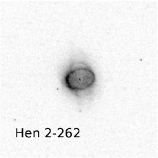
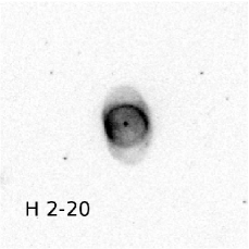
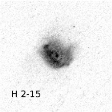
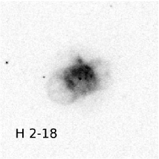
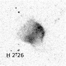
From this observed sample, for the 3D analysis we selected objects which appear similar and exhibit both axial-symmetry and point-symmetry. These PNe show both a central structure (which can be interpreted as an equatorial torus) and a pair of rather wide, extended and closed “classic” lobes. Both lobes are the same and oriented perpendicular to the equatorial plane. This criterion is fulfilled by six objects only: Hen 2-262, H 2-20, H 2-18, Hen 2-260, Wray 16-286, and H 2-27. It is not unlikely that some other objects in the complete sample should fall into this group. Round PNe could be bipolars seen along the symmetry axis. However for clarity of this analysis we did not consider these doubtful cases. We added two more objects to the present work: H 2-15 and H 2-26. Because of their morphology and their old age assigned by Gesicki et al., (2014) we suggest that both are in a post-bipolar phase, and thus provide a useful comparison sample discussed later in Sect. 3.7 and Sect. 4.4.2.

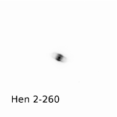
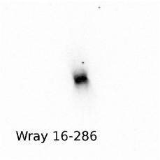
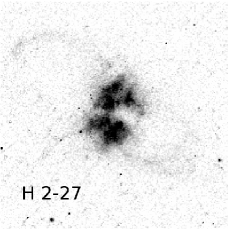
Fig. 1 presents the H$\alpha$ HST images. The intensity is represented as a linear grey scale. The images reveal some details of the bipolar lobes; the lobes are much weaker in intensity than the torus. The angular size of each square is the same (12 arcsec on the side) to visualize the differences in angular size between the PNe. The two proposed post-bipolar PNe are shown in the Fig. 1 in the right-most column.

The selected emission lines are shown in the right columns of Figs. 3–10 together with the fitted models. The spatial resolution of the UVES data is much lower than that of HST: the slit was 0.5 arcsec wide and the seeing was about 1 arcsec (typically between 0.6 and 1.4 arcsec, for H 2-27 even above 2.5 arcsec). For the analysis of the line profiles, the central arcsecond was extracted from the observed slit spectra. Thus, the analysed line profiles are those observed near the centre of each nebula. This suffices to derive the velocity of the inner regions, but the far-away tips of the lobes lay beyond the long-slit so that the extremum velocity is not as well constrained by the observations.

2.2 pyCloudy and 3D photoionization modelling

The pyCloudy code (Morisset, 2013) used for the modelling is available on a web page together with documentation and instructions. It consists of a photo-ionization code (for which Cloudy (Ferland et al. 2013) is used) and a python library that contains routines to analyse the models. Included are routines to visualize the models, to compute the (differently defined) averaged expansion velocities, to integrate the masses, fluxes etc.

As already described this method of solving for the structure is pseudo-3D rather than full 3D. The python codes in their current version limit the modelling to axial- and point-symmetric objects. The photo-ionization models are themselves 1D, and therefore do not consider correctly the effect of the diffuse radiation field. The interpolation introduces further uncertainties. It is however computationally fast. Full models, e.g. using Monte Carlo methods (see for example Danehkar et al., (2013)), are computationally very expensive. In the current work we will explore whether the data can be fitted with the pseudo-3D models. Full 3D models are left for later.

We will use a blackbody spectrum for the central star, as was done in previous 1D models. These models tend to return a lower stellar temperature than using model atmospheres, because they lack the Lyman jump. We ran several tests comparing blackbody SED with the stellar atmospheres SED available at Cloudy web page, in particular with the PN central star models of Rauch, (2003) and found that this had no significant effect on the velocity fields and ages. The adopted blackbody temperatures $T_{\mathrm{bb}}$ are listed in Table 1.

2.3 Density structure

The photoionization part of pyCloudy computes a sequence of one-dimensional regular Cloudy models aimed to represent the structure of a single nebula diagnosed at many different radial directions. Each 1D model actually represents a spherically symmetric PN and consists of an empty inner region extending from the centre up to the specified inner radius, then follows the main nebular body at a constant density, and terminates at the specified outer radius or at the ionization boundary, whichever comes first. Produced are 1D grids of line emissivities, electron temperatures, etc.

Each computed 1D model corresponds to a selected radial direction, inclined to the equatorial plane at a specified (latitudinal) angle with varying inner and outer radii. In our models, the first is at $0\degr$ (equator) and the last at $90\degr$ (symmetry axis). The angles in between are selected based on the structure of each nebula, and are different for each model. The spacings do not need to be uniform in angle. We used 8 separate angles, based in part on the required computational time. A test run with a set of 16 angles showed little improvement, and for our structures sets of 8 angles appear to be sufficient.

pyCloudy re-grids the obtained 1D distributions into a XZ cross-section of a 3D cube. Because of the introduced symmetry centre and symmetry axis only one quadrant of the plane needs to be filled. The space between the 1D lines is filled in by interpolation while the remaining quadrants of the cross-secting plane are filled in by symmetry conditions. These planes are shown for each analysed object in Figs. 3–10 in the upper-left panels. The symmetry axis is placed horizontally. The gas density is shown in grey shades in linear scale but plotted only for the ionized part of the nebula. In one quadrant the (magenta) line segments indicate the eight directions along which the 1D Cloudy models were computed. The outer end of each segment corresponds to the assumed end of gas distribution i.e. the matter (density) boundary. Wherever the shown density is not reaching the line-segment’s end this means that in this direction the actual nebular edge is defined by the ionization front.

The full cube is filled by pyCloudy through rotation around the symmetry axis. To fill the cross-secting plane and the full cube the standard linear interpolation of python was applied. Routines are available to compute the projection of the full cube onto the plane of the sky, defined by the inclination angle between the line of sight and the symmetry axis. In this way model images can be obtained for any of the calculated emission lines. For H$\alpha$ they are shown in Figs. 3–10 in the centre-left panels. Very different nebular structures can be obtained through varying the shapes of the inner voids and outer lobes.

The computed images are compared visually with the HST images (shown in Figs. 3–10 in the bottom-left panels) and then by trial and error the inner and outer radii, the inclination of the symmetry axis, the densities and latitudinal angles of the individual sectors are optimized. Their numerical values are given in Table 2.

2.4 Velocity field

A velocity field is defined where all velocities are directed radially with respect to the central star, and the velocity only depends on the radial distance from the centre. Note that this is simpler than the density structure: the material has different spatial distribution at different latitudinal angles while the velocity distribution is the same for any inclination. More complex velocity fields (depending e.g. on the angular distance from the symmetry axis) are possible but go beyond the scope of this paper, or the observational constraints.

A constant expansion velocity is inconsistent with the different widths of lines of different ions, which indicate higher velocities in the outer (low ionization) regions. To limit the number of the model free parameters, the velocity was restricted to be linearly increasing with radial distance, starting from zero at the central star and reaching a maximum at the ends of lobes. This Hubble-type dependency (alternatively often called homologous) improved the model. Trial computations showed a need to further modify this simple scheme. We introduced an inner region with a constant velocity. Thus, the adopted velocity fields are composed of an inner plateau (its velocity and radial extent was adopted by trial and error, guided by the [O iii] 5007 Å line profile), connected to the linearly increasing part further out (guided by the [N ii] 6583 Å line). The spherical symmetry of the velocity field combined with axial and point symmetry of the density distribution provides a slow expansion for the dense regions close to the star (dominated by the equatorial torus at low inclination angles) and fast expansion for the far-away extended and thin lobes at high inclination angles.

We stopped at this level of complication. Such a situation appears reasonable for 3D bipolar models and corresponds quite well to many of the 1D models (composed of a dense inner shell and an extended outer halo e.g. Gesicki et al., (2014)). Such velocity is in agreement with “a typical middle-aged and fully ionized nebular structure” obtained with the 1D hydrodynamical modelling of Schönberner et al., (2014). Even better agreement is with the 2.5D hydrodynamical calculations of Huarte-Espinosa et al., (2012) where some of the models show a Hubble-type expansion combined with closed bipolar lobes.

Our velocity field is also similar to those found observationally for bi-lobed nebulae. For the well-resolved nebula NGC 2346 at a distance of 700 pc, Arias et al., (2001) derived a best model with “outflow velocity directed radially and proportional to the radial distance”. The NGC 2346 expansion velocities of 16 km s^-1 at the central ring and of about 60 km s^-1 at the tips of the lobes are comparable to many of our values. For two other nebulae, NGC 6302 (Szyszka et al., 2011) and NGC 7027 (Walsh et al. 1997) also similar velocity fields were found although both objects have a rather dramatic appearance. Alcolea et al., (2007) analysed molecular gas in the pre-planetary nebula M 1-92 (Minkowski’s footprint) and found a Hubble-like velocity field not only in bipolar flow but also in the equatorial plane. Note that this situation is neither new nor unique and is typical to our whole sample.

Line profiles can be calculated by integrating the particular line of sight through the cube, at any position within the projected image. Summing these over a defined area simulates the line profile obtained through a slit. The spectrograph slit is assumed in the shape of a rectangle around 1.5 arcsec on the side. This includes the effect of seeing. Positioned centrally on the nebular image, this produces symmetric line profiles. However when the rectangle is shifted somewhat off-centre, calculations show an asymmetric profile. This effect is well known, see e.g. Monteiro et al., (2000). The asymmetry obtained in this way fits quite well to the observed spectra and this was done for some of our objects. In Figs. 3–10 in the middle-left panels we indicate with the (red) rectangle the applied size of the slit superposed on the projected nebula image. The right panels show the computed line profiles (dashed red lines) obtained with this setup.

However, there is an ambiguity: we cannot tell whether the observed asymmetry comes from a slight offset of the spectrograph slit (which for extended weak objects is very likely) or from real irregularity within the nebulae themselves (which the images indicate is also present in some cases).

2.5 Inclination angle

The derivation of geometrical dimensions and of the expansion velocities for bipolar PNe is much more complicated than for spherical ones. The angle of inclination between the polar axis and the plane of the sky affects several parameters and requires special attention.

Figure 2: Emission line profiles for different inclination angle. Plotted is the [N ii] 6583 Å line computed for the model of the spatially unresolved nebula Hen 2-260. The solid line represents the inclination angle of $0\degr$ (symmetry axis within the plane of the sky), long-dash line – inclination of $30\degr$, short-dash – of $60\degr$.

The dominant part of the line emission originates in the dense nebular torus. If the symmetry axis lies in the plane of the sky then most of nebular material moves towards to and away from the observer and the resulting emission profile is clearly split, with a dip at the systemic velocity. At the other extreme, when the torus lies in the plane of the sky the bulk expansion proceeds perpendicularly to the line of sight, the line narrows and the splitting disappears. The observed splitting of the brightest part of the line profiles can be used to derive the best-fitting inclination of the symmetry axis of the model as illustrated in Fig. 2. This figure was plotted for [N ii] 6583 Å line of Hen 2-260 for inclination angles of $0\degr$, $30\degr$ and $60\degr$. This plot can be compared with Fig. 6 bottom-right panel where an inclination of $50\degr$ was adopted. The nebula is spatially unresolved by the spectrograph therefore the behaviour shown in Fig. 2 does not depend on the selection resulting from an applied small slit area. This kind of analysis is possible thanks to the high spectral resolution (about 5 km s^-1) and this example shows that the accuracy of the inclination of such a procedure can be roughly estimated as $\pm 10\degr$.

However the splitting depends also on the assumed velocity field. Further, the derived inclination angle determines the true extent of the model which is used in the velocity field.

Another effect can be deduced from Fig. 2: with increased inclination angle the low-intensity and high-velocity line wings become apparent. This follows from the fact that for the highly inclined object the extended fast lobes expand in the direction closer to the line-of-sight and the emission becomes Doppler-shifted. Because of this effect the lobes are partially available for the kinematical reconstruction even despite the limited spectrograph slit area. For the angles of about $40\degr-50\degr$ quite a significant part of the velocity field can be probed. However for smaller inclination angles and larger nebulae the lobe’s velocity has to be extrapolated with the assumed homologous expansion law derived based on the central regions. Certainly ‘integral field unit’ spectroscopy would provide data much better suited for this kind of analysis; nevertheless even this would not help to measure the gas motions in the plane of the sky.

All these factors introduce a type of degeneracy. The degeneracy is reduced by the restriction to linearly increasing velocity fields and ellipsoidal shapes. Careful examination of details of the images and spectra assures us that the model is a good proxy for the real nebulae but each solution may not be unique.

3 pyCloudy models for individual objects

Figure 3: Hen 2-262. The top left panel shows the assumed density structure for the ionized nebula only, drawn at the cross-section plane taken along the positioned horizontally symmetry axis. The (magenta) lines indicate the directions along which the 1D constant density Cloudy models were calculated. The end of each line segment corresponds to the assumed matter (density) boundary. The middle-left panel shows the H$\alpha$ image (i.e. a projection onto a plane of the 3D structure) obtained for the same model but inclined to the sky plane at $20\degr$ to correspond approximately to the HST image, shown in the bottom left panel (also in Fig. 1). The intensity grey scale is linear in all three images, the size is scaled to fill the width of the box. The (red) rectangle in the middle panel indicates the area over which the line profiles are integrated. The nebular emission line profiles are shown on the right, the solid (black) lines show the observations while the dashed (red) lines show the computed model, for H$\alpha$, [O iii] 5007 Å, and [N ii] 6583 Å.

Figure 4: H 2-20. Data presented as in Fig. 3. The axis inclination is $30\degr$.

Figure 5: H 2-18. Data presented as in Fig. 3. The axis inclination is $35\degr$.

Figure 6: Hen 2-260. Data presented as in Fig. 3. The axis inclination is $50\degr$. The spectrograph slit (left middle panel) covers the whole nebula.

Figure 7: Wray 16-286. Data presented as in Fig. 3. The axis inclination is $20\degr$.

Figure 8: H 2-27. Data presented as in Fig. 3. The axis inclination is $35\degr$.

Figure 9: H 2-15. Data presented as in Fig. 3. The axis inclination is $45\degr$.

Figure 10: H 2-26. Data presented as in Fig. 3. The axis inclination if $40\degr$.

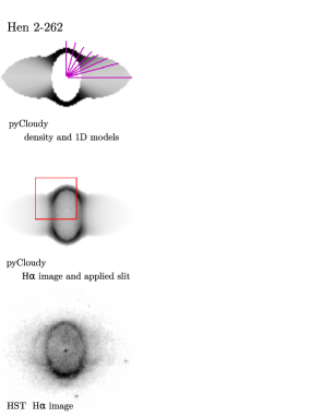
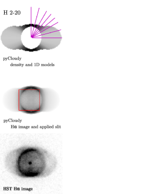
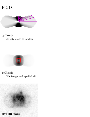
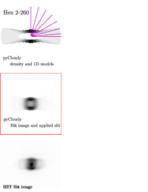
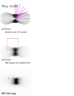
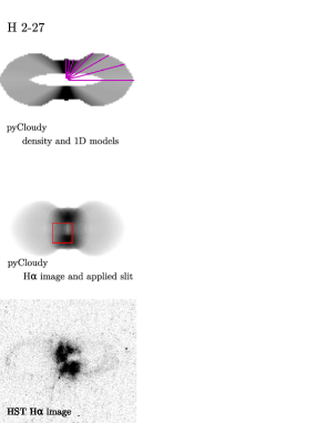
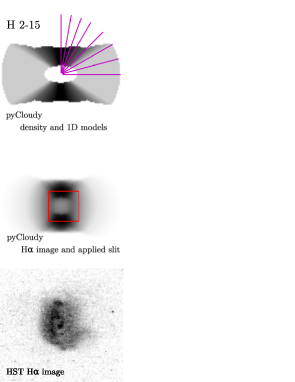
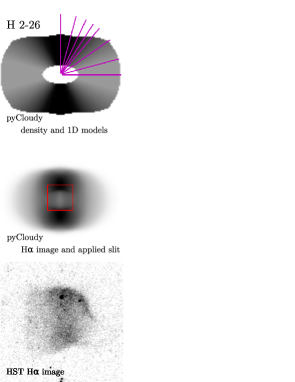
Table 1 lists the parameters of the photo-ionization models for the program nebulae. The Galactic bulge distance was assumed by default however two objects discussed below were considered lying outside the bulge. The stellar blackbody temperature $T_{\mathrm{bb}}$ was adopted from previous Torun models (Gesicki et al., 2014). We checked that major modifications were not necessary to improve the fits, however we did allow for minor corrections. The stellar luminosities were adopted to fit the nebular H$\beta$ fluxes. In some cases these luminosities were smaller than predicted by the evolutionary tracks what Gesicki et al., (2003) interpreted in terms of photon leakage through transparent parts of the nebulae. In the axially symmetric objects the low-density and low-opacity lobes are easily identified as responsible for such leaking therefore the luminosity values should be regarded as lower limits to the true stellar values.

For the line strengths and ratios we list the observed and the pyCloudy values. The observed values are taken from the literature and relate to the entire nebula. The H$\beta$ fluxes are fitted well because the densities and luminosities were varied to obtain that fit. The two most representative strong lines are fitted with an average error of about 25% (in two extreme cases reaching 60%) which is actually not larger than in the old Torun models. The chemical abundances are taken from the Table 7.2 (column “Planetary”) of the Cloudy C13.1 documentation available at the web page which assume solar-like metallicities. For N and O wherever possible we changed the values to the available estimations for individual PNe – these data are given in the Table 1.

The ionized mass is defined as the mass of the region where hydrogen is ionized, and includes both the ionized and neutral helium in this region. For each object, two values of the ionized masses are listed: the (1D) Torun and the pyCloudy model. The difference between them is discussed in Section 4.1.

The values of the inclination angles between the sky plane and the nebula symmetry axis are presented in Table 2 and in figure captions for each of the discussed objects. In Figs. 3–10 we present the influence of the inclination angle on the observed image: the upper left boxes show the density distribution over the full length of the model while the middle left boxes show the H$\alpha$ image obtained for the same model but now with the long axis inclined to the plane of the sky. Depending on the assumed angle the effect is more or less visible. These images correspond to the (appropriately rotated) HST images shown in the lower left boxes. This double presentation illustrates better the intrinsic model structure versus the observed structure of the nebula.

3.1 Hen 2-262 ( PN G001.2+02.1)

The Torun model of Hen 2-262 was not previously published and therefore its parameters are not compared with pyCloudy in the Table 1. It was observed with the same set-up together with the whole Galactic bulge sample however it was not included in the analysis of Gesicki et al., (2014) because the complicated velocity field required significant turbulent motions in the 1D model. The pseudo-3D model shown in Fig. 3 is acceptable, moving the slit off-centre improved the fit but it still appears that adding some turbulence would broaden the line wings and reduce the central splitting in better agreement with observations. However, the presented model is with a simple, linear velocity field.

The density contrast between equator and pole is a factor of 5.6. The model is radiation bounded in the equatorial torus while the lobes are matter bounded.

3.2 H 2-20 ( PN G002.8+01.7)

The best fitting pyCloudy model (see Fig. 4) has an equator-to-pole density contrast of a factor of 5. The model is radiation bounded in all directions.

The emission line profiles show the presence of an ionization gradient within the PN, which is usually associated with the presence of the radiation boundary, i.e. ionization front. A small offset of the artificial slit assumed at the line profile computations resulted in asymmetric lines which resemble the ones observed. Nevertheless in Fig. 4 more asymmetry can be seen in the observed profiles which cannot be fitted with cylindrical-symmetry models.

The 1D model of Gesicki et al., (2014) predicted a velocity field which is monotonically, almost linearly, increasing outwards with a small plateau in the inner region. This is very similar to the velocity field derived in this work.

3.3 H 2-18 ( PN G006.3+04.4)

The best-fitting model has a high equator-to-pole density contrast of a factor of 11. The [N ii] 6583Å line is very weak: any model with an ionization front predicts this line an order of magnitude too strong. The observed line ratios are best reproduced with a model which is matter bounded and has low densities. However at these low densities there is no ionization gradient within the nebula which is in contradiction with the observed emission profiles. We built a compromise model which is still matter bounded in all directions but with a density of the equatorial torus high enough to show an ionization gradient within the nebula.

The shape of the three emission lines is reproduced reasonably well, including the unusual quadruple [O iii] 5007Å line. However, the details of [N ii] 6583Å cannot be better tuned within the simple model. The 1D model of Gesicki et al., (2014) predicted a linearly increasing velocity field.

3.4 Hen 2-260 ( PN G008.2+06.8)

The equator-to-pole density contrast is a factor of 7. The best fitting model (see Fig. 6) shows a larger than average inclination: this is required to reproduce the lack of splitting in the [N ii] 6583 Å line profile. The nebula is radiation bounded, except for a narrow cone along the symmetry axis where it is matter bounded.

This object was discussed in Hajduk et al., (2014), where it was analysed with spherically symmetric (1D) Cloudy and Torun codes. They derived a distance to this PN of 12 kpc. We adopted this value, and also took the other parameters from Hajduk et al., (2014). The object was also in the sample of Gesicki et al., (2014), but there it was assumed to be at the distance of Galactic bulge and therefore a smaller radius was used. The low radial velocity of Hen 2-260 (Durand et al. 1998) is consistent with a non-bulge location. Fig. 1 shows that Hen 2-260 is much smaller than the other PNe which is understandable if it is located beyond the Galactic bulge (Bensby & Lundström 2001).

The line ratios are rather well reproduced by pyCloudy using a blackbody $T_{\mathrm{eff}}=26\,000$ K. Hajduk et al., (2014) used a stellar atmosphere model which requires a higher temperature for the same number of ionizing photons: they find 35 000 K. Hajduk et al., (2014) derived the age of this PN with a direct method (from the heating rate of the central star): their age (980 yr) approximately agrees with that estimated below from the kinematics.

The 1D model of Gesicki et al., (2014) predicted a parabolic shape for the velocity field, with an average expansion velocity somewhat smaller than the 3D estimation presented here. The linear velocity field used here provides a reasonable fit to the line profiles, but there are slight discrepancies in the widths of the various lines. Any further improvement would require a more complex velocity field.

3.5 Wray 16-286 ( PN G351.9-01.9)

The equator-to-pole density contrast of the best model (see Fig. 7) is high, at a factor of 9.3. The model is radiation bounded in the equatorial torus whilst the lobes are matter bounded.

The old 1D Torun models indicated a parabola-like velocity field with mass-averaged velocity of 13 km s^-1. This yields an age that is significantly larger than pyCloudy: we found that the parabola minimum is responsible for the difference. The pyCloudy model reproduces line profiles much better and the narrow [O iii] 5007 Å and wide, flat-topped and slightly asymmetric [N ii] 6583 Å are explained by the spectrograph pointing off-centre with the slit not covering the midpoint. The pyCloudy model results in a higher average velocity of around 20 km s^-1 (dependent on the weighting method used in the averaging).

3.6 H 2-27 ( PN G356.5-03.6)

The best fitting model (see Fig. 8) gives a high equator-to-pole density contrast, of a factor of 7.9. The model assumes a spectrograph slit position which is a little offset, in order to reproduce the small asymmetry observed in profiles. The model is matter bounded in all directions.

For this PN we assumed a smaller distance than to the bulge. Although reasonable photoionization models can be built for different distances, some aspects point towards a smaller value. In Fig. 1 this PN is shown to have the largest angular dimensions. Durand et al. (1998) report a low radial velocity which does not require a bulge location. The correlations discussed below suggest that H 2-27 has a smaller kinematical age. The velocity is derived from spectra i.e. independently from distance; therefore the age can be reduced by decreasing the physical radius and therefore the distance. Having no more constraints we simply assumed the distance of 4 kpc for the pyCloudy models. For H 2-27 we recomputed the Torun model for the smaller new distance, previous Torun models which assumed bulge distance resulted in larger age for this PN.

The 1D model of Gesicki et al., (2014) predicted a linearly increasing velocity field.

3.7 Two post-bipolar nebulae: H 2-15 ( PN G003.8+05.3) and H 2-26 ( PN G356.1-03.3)

These two nebulae have a more irregular structure than the others, and are suggested to be in a post-bipolar phase of evolution. They have numerous common characteristics and they are included here for comparison. The models are shown in Figs. 9 and 10.

The models show a relatively low equator-to-density contrast of a factor of 5 and 2.5 for H 2-15 and H 2-26 respectively. They have lower density than the other objects peaking at around $10^{3}$ cm^-3. Both models are composed of a thick disk which is radiation bounded in the directions near the equatorial plane whilst directions towards the poles are matter bounded. For both, the lowest stellar luminosities were derived so they can be the most transparent for stellar ionizing radiation (most leaking). Both were fitted with linear velocity fields in Gesicki et al., (2014). The 3D pyCloudy resulted in a very similar averaged velocities. For these two PNe Gesicki et al., (2014) built models with attached a low density halo to the dense shell: this improved the fit of the [N ii] 6583Å line but in consequence increased the outer radius and the age. The pyCloudy models assume for both nebulae that the artificial spectrograph slit is a little offset, to reproduce the asymmetry observed in profiles. However, the images also show significant asymmetries. The kinematical ages derived here are smaller than those derived in Gesicki et al., (2014), but are still two times larger than the ages of the six bi-lobed PNe.

4 Discussion

4.1 Ionized masses

For all objects the pyCloudy masses (presented in the Table 1) are smaller than those from the 1D Torun models, in most cases (6 out of 8) by a large factor of 2–7. In two cases are the masses nearly the same. The dominant effect is the use of a 3D versus a 1D structure. A 3D model provides for a range of density distributions within one object.

The H$\beta$ emission being proportional to the density squared (actually $n_{\mathrm{p}}\times n_{\mathrm{e}}$) is dominated by regions of high hydrogen density. This gas has different spatial distributions in the spherical and the pseudo-3D models, being a compact sphere or a torus respectively. Despite these differences the densities and overall masses of those regions are comparable and produce the same H$\beta$ fluxes. Much larger are the differences in the distributions of low density gas. In spherical models the low density gas occupies the large volume of the spherical halo which sums up to a significant fraction of the total nebular mass.

Another contributing factor is the irradiation of the outer regions. In 1D models, the radiation reaching the outer regions first passes through dense inner layers and the attenuation gives a much reduced intensity. To reach a significant line strength of the low-ionization lines (which arise in the outer regions), a larger amount of gas is required. In 3D models, there are directions in which the outer regions are illuminated by radiation which has passed through little intervening gas. Thus, less gas is needed to reproduce the line strengths.

This important result shows that ionized masses of planetary nebulae have very large uncertainties attached. 1D models are best viewed as giving upper limits to the mass. Pseudo-3D models provide a better approximation to true nebular ionized masses.

The total mass lost by the central star might be somewhat larger than the models ionized mass because we do not know how much neutral material exists in the dense equatorial disk beyond the ionization boundary.

4.2 Averaged expansion velocities

The true velocity distribution within a planetary nebula can in principle be quite complicated. The current analysis considers only the large-scale flows which in our paper are only approximated, as described in Sect. 2.4. Further simplification is related to limiting the velocity to be a function of radius only, and not of latitudinal angle. Defining a single-valued expansion velocity for a non-constant velocity field requires a weighting. The velocity at the outer radius (or ionization front) is typically not useful, as it is not directly measured: the available emission lines come from a region a bit further in (e.g. the ‘post-shock’ velocity discussed by Jacob et al., (2013)). For 1D models, the mass-averaged expansion velocity (Gesicki & Zijlstra 2000) has been shown to be a robust parameter. It represents the bulk motion, and is easily and reproducibly measured from the models, even where very few emission lines are available.

For the 3D models, there is not yet a similar methodology. We investigate two options: weighting by mass (similar to the 1D models) and weighting by the H$\beta$ emissivity. Weighting by mass has the draw-back that the pyCloudy models use constant density (for each direction). This gives a high weight to the outermost radius, where velocities are highest but neither the densities nor the velocities are well constrained. The H$\beta$ emissivity decreases outwards tracing the ionized mass distribution. Weighting by H$\beta$ emissivity gives smaller weight to the outer radius – a behaviour closer to the 1D Torun models, where the density decreased towards the outer radius.

Table 1 lists the averaged expansion velocities $<V_{\mathrm{exp}}>$ and nebular radii together with the corresponding 1D Torun model values. Both averaging methods are compared in Fig. 11, plotted versus old Torun model values. Filled symbols represent weighting by H$\beta$ while open symbols weighting by mass distributions. The circles (red) show the bipolar objects, the squares (blue) – the probable post-bipolars. The pyCloudy mass-averaged velocities are higher than the H$\beta$-averaged velocities – exactly as expected. However note that in either case, the result is dominated by the torus where most of the gas is located.

Figure 11: Averaged expansion velocity from Torun models compared with pyCloudy. The abscissa shows the Torun models mass-averaged velocities, while at ordinate the pyCloudy H$\beta$-averaged values are shown as filled symbols, and the pyCloudy mass-averaged as open symbols. The (red) circles show the bipolar nebulae and the (blue) squares the post-bipolars. Data from Table 1.

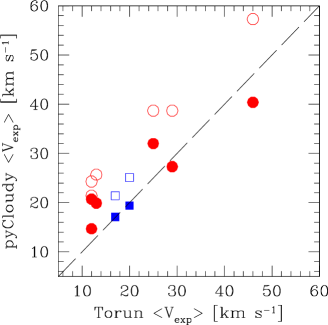
Comparing the values of $<V_{\mathrm{exp}}>$ from pyCloudy averaged by H$\beta$ with the values of $<V_{\mathrm{exp}}>$ from Torun models averaged by mass indicates a good correspondence (see Fig. 11). We conclude that the averaged velocity remains a robust parameter to describe a planetary nebula. Because of the rather scarce observational and hydrodynamical data to compare with, for the simplified models used here, weighting by the H$\beta$ line emissivity is preferred over weighting by mass.

Figure 12: Averaged expansion velocity vs. averaged outer radius for the pyCloudy modelled PNe. Velocity are H$\beta$-averaged and the outer radius is mass averaged (see text). Data from Table 1. The filled circles show the bipolar nebulae and the filled squares the post-bipolars.

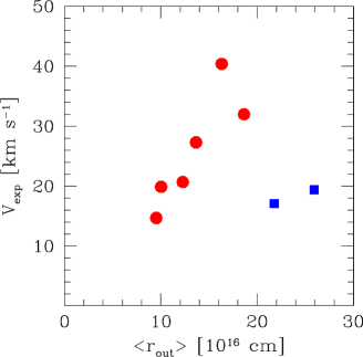
In Fig. 12 we plot the velocities versus the outer radius radii. The velocities shown are H$\beta$ averaged wile the outer radii are mass-weighted. The circles represent the bipolar nebulae. They show almost linear relation. The two PNe tentatively classified as post-bipolar are represented by squares: they have the largest radii but also show low expansion velocities.

4.3 Kinematical ages

The kinematical age can be derived from the (averaged) expansion velocity and the outer radius. However, this only provides an approximation. The ionization front travels faster than the gas velocity: the gas density declines as the nebula expands, allowing more gas to become ionized. The velocities can become very fast at the ionization front, due to the over-pressure. To quantify the effects requires hydrodynamical models. Based on the hydrodynamical models of Perinotto et al. (2004), in the 1D case the kinematical age should be reduced by a factor of 1.4 (Gesicki et al., 2014).

For 3D models the derivation is more complicated. First, there is no unique outer radius. Second, the torus and the lobes may also have different ages. Third, the correction factors from 1D hydrodynamical models may not be directly applicable to a non-spherical 3D structures, where pressure gradients may cause non-radial velocities. Because of these uncertainties, we focus on deriving limits to the ages.

An upper limit can be obtained from the outer radius and the expansion velocity of the torus. We calculate the mass-averaged outer radius of the ionized nebula. This is dominated by the dense torus; the value of $<r_{\mathrm{out}}>$ is listed in the Table 1. We divide this radius by the H$\beta$ weighted expansion velocity to obtain an age. The H$\beta$-averaged value is used because it is smaller than the mass-averaged value, and therefore yields a larger age. This age is listed as ‘nebula’ age, and should be considered an upper limit. No correction factor other than the averaging has been applied. For comparison, the 1D Torun model ages are also listed: for these the correction factor of 1.4 has been used (Gesicki et al., 2014; Schönberner et al. 2005).

A lower limit can be obtained from the lobes, which are expected to be younger than the main nebula (Huggins 2007). The linear velocity field indicates a Hubble-type flow in the lobes. The inherent feature of homologous expansion is the same age derived at any distance therefore the exact estimation of the extent of the lobes is not an issue. We assume that no acceleration or deceleration has taken place and obtain the age for the tip of the lobes. These ages are listed as ‘lobe’ age in the Table 1.

Our ‘nebular’ age is different from the Hubble-type age of the lobes. The homologous expansion does not start from zero at the centre: there is assumed a dense and constant-velocity inner region and the applied averaging is biased towards this low-velocity region. Encouragingly, the upper limits are always higher than the lower limits. The upper limits are in most cases close to the 1D Torun ages.

4.4 Evolution

Figure 13: Averaged expansion velocity vs. kinematical age for the pyCloudy modelled PNe. The filled symbols show the nebular ages (derived from radii and velocities shown in Fig. 12), and the open symbols the lobe ages (see Sect. 4.3). Circles show the bipolars and squares the post-bipolars.

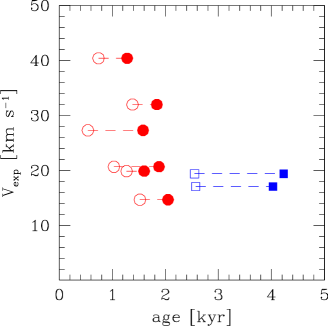
The aim of this work was to test for possible evolutionary sequences among our objects. Fig. 13 shows the expansion velocity versus the kinematical age. The open symbols show the ages of the lobes, and the filled symbols the nebular ages. The latter is defined as above and may be considered as upper limits. All bipolar PNe occupy a narrow region in age, in the range 1–2 kyr. Some of the lobes are a bit less than 1 kyr. The nebular ages are 0.5–1 kyr higher than the lobes. For the two post-bipolars, the lobes are 2.5 kyr old; their nebular ages are around 4 kyr, a much larger difference than for the bipolars.

4.4.1 The six bipolar PNe

The interesting result is that the selected bipolar PNe have nearly the same age (see Fig. 13). However their central star temperatures are spread over a wide range. This may indicate a range of stellar masses (higher mass stars evolve faster to higher temperature). This result suggests that the lobes may form at a well-defined point during the nebular expansion, independent of stellar mass.

None of the selected bipolars are older than 1.5–2 kyr. A sample of six objects is too small to draw any general conclusions, but this may point at a fading time for the lobes. A short window of visibility for bipolar lobes would have consequences for their rate of occurrence. The visibility time of the nebulae within the size range selected for HST (5 arcsec or less) is 3–4 kyr (Gesicki et al., 2014, their Fig. 11) (assuming the accelerated Schönberner tracks). This is a general visibility time which does not depend on the nebular structure. Our sample of 6 represents 17% of the sample of compact PNe observed with HST. The lobes can be seen for about half of the total visibility period. Correcting for this, we find that 30%–35% of the compact bulge PNe may experience a bipolar phase. This number can be higher if it would be possible to identify the bi-lobed PNe seen along the symmetry axis.

Our conclusion concerning ages is not unique among related objects. Huggins (2007) has shown that jets and tori in post-AGB stars have very similar ages, with jets being younger by a few hundred years. The expansion times range from a couple of hundreds to a couple of thousands years and the torus pre-dates the jet. This was also found for the torus and lobes of NGC 6302 (Szyszka et al., 2011), where the lobes are younger by $\sim$600 yr from the 2900 yr old torus. The pre-PN M 1-92 (Alcolea et al., 2007) kinematical age of 1200 yr (the same in polar and equatorial directions of a bipolar molecular outflow) is also very similar to our data.

4.4.2 The two post-bipolar PNe

In the sample of 36 PNe we tried to identify possible descendants of the bipolar PNe. We searched amongst the oldest from the data of Gesicki et al., (2014). Two objects seem to be the likely candidates, namely H 2-15 and H 2-26. Both are older than 3.5 kyr (among the four oldest), both have very hot central stars (supporting their evolutionary advanced status), and both show morphologies resembling a torus, already well expanded, with evidence for fragmentation. They also reveal interactions with the interstellar medium. Some faint structures might be the remnants of bipolar lobes. The derived velocity fields contain a linear part, consistent with residual lobe emission. However, more detailed observations would be needed to confirm this.

For both PNe the pyCloudy models confirmed their old kinematical age although the new ages are somewhat smaller. Both are larger than the classic bipolar PNe (Fig. 12) and approximately two times older (Fig. 13).

Their expansion velocities are low. The velocities may be biased due to the weakness of the lobes. However it is not unlikely that these two are descendants of the subgroup of slow expanding PNe, while the objects which expand faster after a couple of thousand years evolve beyond detection limit. But this could be as well a result of the limited sample and we just see such two objects.

Some hint concerning the evolved nature and the timescales of similarly looking PNe can be found in Manchado et al., (2015) where a sequence of hydrodynamical models has been presented, intended to explain the clumpy structure observed in PN NGC 2346. The published cross-sections through the nebular emission measures (unfortunately not the rendered images) show how the equatorial toroid breaks up into clumps already about 1000 yr after the decline of the fast stellar wind which earlier produced the bipolar lobes. That is interestingly similar to our post-bipolar objects.

It cannot be proven that the two PNe form late stages of bipolar evolution. But in view of the short visibility time of bipolar lobes, the presence of such objects in the bulge sample would be expected. As noted in the previous subsection the phase of symmetric lobes lasts about half of the total visibility time, so the other half can appear like these.

5 Conclusions

• We selected targets from the HST survey of 36 compact bulge PNe, not constrained on brightness or morphology. Six PNe in the sample have clear bi-lobed, axi-symmetric structure suitable for pseudo-3D modelling. Two further targets are possibly in a post-bipolar phase. Most of the targets are believed to be at the distance of the Bulge, at 8 kpc, two of them are modelled at distances of 12 kpc and 4 kpc.

• The pyCloudy models are able to fit the available constraints. The constant density per segment, and the simple velocity field, limit the accuracy but also keep the number of free parameters reasonable.

• The 3D models yield much lower ionized masses than the 1D models, typically reduced by a factor of 2–7. We find ionized masses in the range 0.02–0.1 $M_{\sun}$. This is an important result with implications for the evolution of planetary nebulae.

• The spectra are successfully reproduced with a linear radius-velocity relation in the outer regions. This simple modelling recipe appears in agreement with hydrodynamical calculations of Huarte-Espinosa et al., (2012) and with a very detailed analysis of the bipolar PN NGC 6302 by Szyszka et al., (2011). We caution that the current models did not explore a wide range of velocity fields, and the spectra were extracted at the central position of the nebula.

• Averaged expansion velocities derived from the pyCloudy models are similar but not identical to the 1D models. Weighting the velocity field by the H$\beta$ line emissivity is preferred over weighting by mass, due to the limitations on the density distribution in this work. The average expansion velocity ranges from 15 to 30 km s^-1, with one object (H 2-18) expanding at 40 km s^-1.

• We derive ages for the lobes based on the model Hubble flow ranging from 500 to 1500 yr. The two post-bipolar show older lobe ages, of 2500 yr. The lobe ages provide lower limits to the age of the nebula. We derive upper limits to this age from the average outer radius and expansion velocity: these range from 1300 to 2000 yr for the bipolars and 4000–4500 for the two post-bipolars.

• The age range of the bipolars is remarkably narrow. The suggestion is that the bright lobes last a relatively short time, and fade after $\sim 1000$ yr.

• We cannot be confident that the two ’post-bipolar’ PNe actual are descendants of bi-lobed objects. However, the derived parameters do not contradict such a relation. A long known hypothesis recently summarized by Frew & Parker, (2012) states that “several stellar evolutionary pathways form objects classified as PNe”. Our morphological selection appears to have picked one such pathway, within which the clear bi-lobed structure can be seen at an early phase at ages of 1–2 kyr while the post-bipolar phase can be identified at ages about 3 kyr, all within the typical total visibility time of about 3–4 kyr. Still we do not know whether this pathway concerns single or binary star evolution.

Appendix A The photoionization model parameters and results

Table 1: Photoionization models parameters and modelling results for the program nebulae. The Galactic bulge distances were assumed by default however for two cases there were reasons to locate them outside the bulge. The temperature and luminosity correspond to the models central blackbody ionizing source. The extinction constants, line fluxes and abundances were taken from literature with the references indicated. Lower part of the table shows the resulting from computations ionized masses, averaged expansion velocities and kinematical ages. For a comparison (discussed in the text) there are given the new values obtained with pyCloudy code and the old values from the published Torun models. The expansion velocity parameter is weighted by H$\beta$ emission and by mass distribution, the old Torun values are only averaged by mass. The nebular outer radius is averaged by mass. The kinematical ages are: ‘lobe’ – the outer lobe radius divided by the velocity at this point, ‘nebula’ – the mass averaged outer radius divided by H$\beta$ averaged velocity.

PN G No.	001.2+02.1	002.8+01.7	003.8+05.3	006.3+04.4	008.2+06.8	351.9-01.9	356.1-03.3	356.5-03.6
PN name	Hen 2-262	H 2-20	H 2-15	H 2-18	Hen 2-260	Wray 16-286	H 2-26	H 2-27
Dist [kpc]	8	8	8	8	12	8	8	4
$T_{\mathrm{bb}}$ [K]	69 600	31 600	80 000	52 000	26 000	83 000	152 000	70 000
$L_{*}$ [$L_{\sun}$]	2040	4070	130	1660	8130	7240	51	100
extinction constant
$C_{\mathrm{H}\beta}$	2.78	2.55	1.08	1.634	0.696	2.58	1.08	2.28
$\log F(\mathrm{H}\beta)$ corrected
observed	$-11.0^{1}$	$-11.0^{1}$	$-12.3^{1}$	$-11.5^{1}$	$-11.4^{6}$	$-10.5^{1}$	$-12.7^{1}$	$-11.9^{1}$
pyCloudy	$-11.0$	$-11.1$	$-12.2$	$-11.6$	$-11.3$	$-10.5$	$-12.7$	$-12.0$
[N ii]6583/H$\beta$ dered.
observed	$0.33^{3}$	$2.81^{7}$	$5.88^{7}$	$0.08^{4}$	$1.06^{6}$	$0.59^{1}$	$6.21^{7}$	$1.58^{1}$
pyCloudy	$0.63$	$3.50$	$3.50$	$0.07$	$0.89$	$0.61$	$7.33$	$1.60$
[O iii]5007/H$\beta$ dered.
observed	$6.99^{3}$	$0.27^{7}$	$9.24^{7}$	$13.00^{4}$	$0.07^{6}$	$10.60^{1}$	$6.28^{7}$	$7.01^{1}$
pyCloudy	$7.33$	$0.42$	$6.02$	$5.24$	$0.15$	$14.30$	$4.60$	$5.58$
chemical abundances
$\log(\mathrm{N}/\mathrm{H})$	$-4.18^{3}$	$-3.40^{7}$	–	$-4.21^{4}$	$-4.35^{6}$	$-3.73^{2}$	–	–
$\log(\mathrm{O}/\mathrm{H})$	$-3.52^{3}$	$-2.74^{7}$	$-3.34^{7}$	$-3.44^{4}$	$-3.31^{6}$	$-3.26^{2}$	$-3.66^{7}$	–
ionized mass [$M_{\odot}$]
Torun	–	0.11	0.15	0.27	0.05	0.25	0.14	0.02
pyCloudy	0.057	0.053	0.039	0.051	0.038	0.097	0.027	0.019
$<V_{\mathrm{exp}}>$ [km s-1] averaged by
H$\beta$ em.	20.7	27.3	17.1	40.4	14.7	19.9	19.4	32.0
mass	24.3	38.7	21.4	57.3	21.4	25.7	25.1	38.7
$<V_{\mathrm{exp}}>$ Torun [km s-1]
	–	29	17	46	13	13	20	25
averaged $<r_{\mathrm{out}}>$ [$10^{16}$ cm]
	12.28	13.65	21.77	16.32	9.52	10.03	25.92	18.64
kinematical age [kyr]
Torun	–	1.56	4.93	1.67	1.61	3.22	3.84	1.63
nebula	1.88	1.58	4.03	1.28	2.05	1.60	4.23	1.84
lobe	1.03	0.54	2.57	0.74	1.52	1.27	2.55	1.38
References:    1 Acker et al., (1992); 2 Chiappini et al., (2009); 3 Escudero et al., (2004); 4 Górny et al., (2009);
5 Gutenkunst et al., (2008); 6 Hajduk et al., (2014); 7 Stasińska et al., (1998); 8 Tylenda et al., (1992).

Table 2: Geometry defining parameters for the program nebulae. The first line shows the inclination angle between the PN long axis and the plane of the sky. Then follow eight groups of lines presenting parameters of each of latitudinal segments out of which the pseudo-3D models are interpolated. The inner and outer radii are in the units of [10¹⁶ cm], the hydrogen number density is in units of [cm^-3].

PN G No.	001.2+02.1	002.8+01.7	003.8+05.3	006.3+04.4	008.2+06.8	351.9-01.9	356.1-03.3	356.5-03.6
PN name	Hen 2-262	H 2-20	H 2-15	H 2-18	Hen 2-260	Wray 16-286	H 2-26	H 2-27
inclination	20$\degr$	30$\degr$	45$\degr$	35$\degr$	50$\degr$	20$\degr$	40$\degr$	35$\degr$
latitude	0$\degr$	0$\degr$	0$\degr$	0$\degr$	0$\degr$	0$\degr$	0$\degr$	0$\degr$
$r_{\mathrm{in}}$	8.9	8.5	5.0	2.0	2.6	1.0	5.0	3.2
$r_{\mathrm{out}}$	10.8	10.5	16.1	11.7	5.5	6.0	21.9	10.5
$\log n_{\mathrm{H}}$	4.2	4.1	3.2	3.65	4.5	4.7	2.9	3.15
latitude	15$\degr$	15$\degr$	10$\degr$	15$\degr$	15$\degr$	10$\degr$	15$\degr$	10$\degr$
$r_{\mathrm{in}}$	8.4	8.5	5.1	2.1	2.8	1.0	5.1	3.2
$r_{\mathrm{out}}$	10.5	10.4	16.1	12.0	5.7	5.7	21.9	10.5
$\log n_{\mathrm{H}}$	4.2	4.1	3.2	3.65	4.4	4.7	2.9	3.15
latitude	30$\degr$	30$\degr$	20$\degr$	30$\degr$	30$\degr$	20$\degr$	25$\degr$	20$\degr$
$r_{\mathrm{in}}$	7.4	8.3	5.2	2.3	3.1	1.0	5.4	3.4
$r_{\mathrm{out}}$	9.9	11.2	17.4	12.3	6.1	6.2	22.7	10.9
$\log n_{\mathrm{H}}$	4.2	4.0	3.2	3.65	4.4	4.8	2.9	3.15
latitude	45$\degr$	40$\degr$	30$\degr$	45$\degr$	45$\degr$	35$\degr$	3$\degr$3	35$\degr$
$r_{\mathrm{in}}$	6.5	8.2	5.6	2.7	3.7	1.0	5.7	3.8
$r_{\mathrm{out}}$	10.5	11.6	18.8	12.6	7.0	6.7	25.0	12.3
$\log n_{\mathrm{H}}$	4.1	4.0	3.1	3.45	4.3	4.6	2.8	3.0
latitude	55$\degr$	50$\degr$	45$\degr$	55$\degr$	60$\degr$	45$\degr$	40$\degr$	45$\degr$
$r_{\mathrm{in}}$	6.0	8.1	6.3	3.3	4.9	1.0	6.0	4.4
$r_{\mathrm{out}}$	13.4	13.7	22.0	20.0	9.4	9.0	27.0	19.5
$\log n_{\mathrm{H}}$	3.9	3.8	3.0	3.2	4.1	4.4	2.8	2.9
latitude	65$\degr$	60$\degr$	60$\degr$	65$\degr$	75$\degr$	60$\degr$	55$\degr$	60$\degr$
$r_{\mathrm{in}}$	5.7	7.9	7.6	4.2	7.6	1.0	7.1	6.1
$r_{\mathrm{out}}$	16.4	17.7	35.4	31.6	25.1	16.7	32.1	25.1
$\log n_{\mathrm{H}}$	3.7	3.6	2.5	3.0	3.4	4.0	2.7	2.7
latitude	75$\degr$	75$\degr$	75$\degr$	75$\degr$	85$\degr$	75$\degr$	75$\degr$	75$\degr$
$r_{\mathrm{in}}$	5.5	7.8	9.1	5.6	10.2	1.0	9.1	10.4
$r_{\mathrm{out}}$	19.8	21.8	35.4	35.3	25.1	20.0	33.1	30.9
$\log n_{\mathrm{H}}$	3.6	3.5	2.5	2.6	3.4	3.9	2.5	2.7
latitude	90$\degr$	90$\degr$	90$\degr$	90$\degr$	90$\degr$	90$\degr$	90$\degr$	90$\degr$
$r_{\mathrm{in}}$	5.3	7.8	10.0	8.0	10.8	1.0	10.0	19.0
$r_{\mathrm{out}}$	24.0	23.5	35.4	39.7	25.1	20.0	33.1	34.7
$\log n_{\mathrm{H}}$	3.5	3.4	2.5	2.6	3.4	3.7	2.5	2.65