Extended Cosmologies

Extended Cosmologies

Salvatore CAPOZZIELLO ${}^{{\dagger}^{1}{\dagger}^{2}{\dagger}^{3}}$, Mariafelicia F. DE LAURENTIS ${}^{{\dagger}^{3}{\dagger}^{4}{\dagger}^{5}{\dagger}^{6}}$,
Lorenzo FATIBENE ${}^{{\dagger}^{7}{\dagger}^{8}}$, Marco FERRARIS ${}^{{\dagger}^{7}}$ and Simon GARRUTO ${}^{{\dagger}^{7}{\dagger}^{8}}$

S. Capozziello, M.F. De Laurentis, L. Fatibene, M. Ferraris and S. Garruto

${}^{{\dagger}^{1}}$ Dipartimento di Fisica, University of Napoli “Federico II”, Italy capozzie@na.infn.it

${}^{{\dagger}^{2}}$ INFN Sezione Napoli – Iniziativa Specifica QGSKY, Italy ${}^{{\dagger}^{3}}$ Gran Sasso Science Institute (INFN), L’Aquila, Italy mariafelicia.delaurentis@gmail.com ${}^{{\dagger}^{4}}$ Tomsk State Pedagogical University, Russia ${}^{{\dagger}^{5}}$ Laboratory of Theoretical Cosmology, Tomsk State University of Control Systems
${}^{{\dagger}^{5}}$ and Radioelectronics (TUSUR), Russia ${}^{{\dagger}^{6}}$ Institut für Theoretische Physik, Goethe-Universität, Max-von-Laue-Str. 1,
${}^{{\dagger}^{6}}$ 60438 Frankfurt, Germany ${}^{{\dagger}^{7}}$ Dipartimento di Matematica, University of Torino, Italy lorenzo.fatibene@unito.it, marco.ferraris@unito.it, simon.garruto@unito.it ${}^{{\dagger}^{8}}$ INFN Sezione Torino – Iniziativa Specifica QGSKY, Italy

Received September 29, 2015, in final form January 16, 2016; Published online January 20, 2016

We shall discuss cosmological models in extended theories of gravitation. We shall define a surface, called the model surface, in the space of observable parameters which characterises families of theories. We also show how this surface can be used to compare with observations. The model surface can potentially be used to falsify whole families of models instead reasoning on a single model basis as it is usually done by best fit arguments with observations.

cosmology; extended theories of gravitation

83F05; 83D05; 37N20

1 Introduction

The aim of this paper is to provide a detailed framework for interpreting extended cosmologies in the family of Palatini $f({\cal R})$-models. The interpretation of extended theories is trickier than usually recognised in the literature, since the dynamics is not sufficient to constrain all details of the interpretation or the relation between the cosmographic parameters and the corresponding model quantities. All interpretation issues are generated by the fact that in Palatini $f({\cal R})$-theories one has two metrics which play a natural role, the original metric $g$ and a conformal metric $\tilde{g}$ which naturally appears when solving the model.

From the geometric point of view, while in standard general relativity (GR) the geometry of spacetime is described by a Lorentzian structure, in $f({\cal R})$-theories spacetime is described by a Weyl geometry, i.e., by a conformal structure $[g]$ together with a compatible connection $\tilde{\Gamma}$ which, in view of field equations, turns out to be the Levi-Civita connection of the conformal metric $\tilde{g}{=\varphi\cdot g}$. The scalar field $\varphi$ is called the conformal factor and it parametrises conformal transformations. Weyl geometries have been considered in the past in gravitational theories; see, for example, [4, 23, 24, 26, 27, 28].

Unlike in standard GR, where one has only one metric which does everything, in Palatini $f({\cal R})$-theories one has to declare which metric is used to do what; see, for example, [1, 2, 7]. For example, the dynamics of field equations does not determine the free fall. If one couples to a matter field of course one can compute the characteristics of matter field equations and argue that characteristic curves describe free fall. In particular, if one couples a Klein–Gordon scalar field $\phi$ to the metric $g$ then characteristics are determined as the geodesics of $g$. Unlike lightlike geodesics, the timelike geodesics of $g$ are not geodesics of $\tilde{g}$. Accordingly, it seems that the free fall is determined by the variational principle assumed for gravity and matter.

However, one can show that a conformal transformation can be extended to act on the matter field $\phi$ as well and define a new matter field $\tilde{\phi}=\varphi^{\alpha}\cdot\phi$ (with the parameter $\alpha\in{\mathbb{R}}$ to be determined) so that the new field $\tilde{\phi}$ obeys new (different) field equations (since conformal transformations are not symmetries of the matter field equations). The exponent $\alpha$ in the action of the conformal transformation on the Klein–Gordon field can be chosen so that the characteristics of the new field $\tilde{\phi}$ are geodesics of the conformal metric $\tilde{g}$; see [18]. Something similar can be done for Dirac fields.

Hence arguing that the variational principle determines the free fall is correct, provided one assumes what is observed as a matter field. Depending on the choice of $\phi$ or $\tilde{\phi}$ as the observed field, then free fall is determined to be described by $g$ or $\tilde{g}$, respectively. In this paper we shall assume that free fall is given by $\tilde{g}$.

Other examples are the issues of whether the dynamics determines the metric which is used for defining spatial lengths, minimal coupling to matter, standard clocks. For example, in standard GR it is natural assuming that physical lengths are associated to the geometric length measured with respect to the only metric one has around, namely $g$. Having more that one metric in the model makes the choice much more problematic.

Let us consider two parallel mirrors at a constant distance and a light ray bouncing between them, which is called a gravitational clock. If one considers an atomic clock (which is in fact built with some quantum harmonic oscillator) and compares its rate to the rate of a gravitational clock, the assumption of standard GR is pretty neat: the two clocks (at the same point) are synchronised forever.

It is quite obvious that the discrepancy between the two clocks, if any, cannot be too big otherwise we shall see some effect at the solar system scales. However, there is no strong constraint on what happens at bigger scales. One should not assume that there is no discrepancy. On the contrary, the correct procedure would be to assume there is, derive observational consequences, and constrain the effects by observations.

We shall hereafter follow this second guideline. In this paper we shall assume that lengths are related to $g$, not to $\tilde{g}$. Accordingly, we shall assume that matter is coupled to $g$, and not to $\tilde{\Gamma}$.

These choices are also motivated by the Ehlers–Pirani–Schild (EPS) framework for gravitational theories; see [14]. In the early seventies EPS proposed a framework able to derive the geometry of spacetime based on basic properties of light rays and (free falling) particles. In this framework one does not assume a Lorentzian structure on spacetime, rather a Lorentzian metric (actually a Lorentzian conformal structure) on spacetime can be defined due to the properties assumed for light rays. As a consequence, in the EPS framework there is a tight link between the geometric structure of spacetime and observations. One could say that the EPS framework instructs an observer to establish observational protocols and to define distances and time lapses. Once this is done EPS considered the properties of particles and find they are described by a connection $\tilde{\Gamma}$ (actually by a projective structure on the spacetime) which describes, by construction, the free fall.

The two structures $([g],\tilde{\Gamma})$ on spacetime are not arbitrary though. Since one knows that lightlike directions are an upper bound for the speed of particles, one can show that the connection $\tilde{\Gamma}$ must be in the form

$$\tilde{\Gamma}^{\alpha}_{\beta\mu}=\{g\}^{\alpha}_{\beta\mu}+\hbox{$\frac{1}{2}$}\big{(}g^{\alpha\epsilon}g_{\beta\mu}-2\delta^{\alpha}_{(\beta}\delta^{\epsilon}_{\mu)}\big{)}A_{\epsilon}$$ (1.1)

for some covector $A_{\epsilon}$. This is quite similar to the original proposal by Weyl for a unified theory of gravity and electromagnetism (then proven wrong); see [28]. However, we are not interpreting here $A$ as an electromagnetic potential and for us the covector $A_{\epsilon}$ will be related to the possible shift in synchronisation between atomic and gravitational clocks.

On the basis of the EPS framework we shall consider gravitational theories for the fields $(g,\tilde{\Gamma})$ to be extended theories of gravitation (ETG) when their field equations enforce as a consequence the relation (1.1); see [10, 11]. We shall call such theories integrable when field equations also imply that $A$ is an exact $1$-form and as a consequence $\tilde{\Gamma}$ is a metric connection; see [13, 16].

In principle one can consider any invariant of the curvature to define a dynamics. We shall hereafter restrict to Palatini $f({\cal R})$-theories in which the dynamics is given in terms of a (regular) function of the scalar curvature ${\cal R}$. One can show that Palatini $f({\cal R})$-gravity is an integrable extended theory of gravitation (iETG). In view of the EPS framework we shall interpret $\tilde{\Gamma}$ as defining the free fall, while $g$ is related to distances and time lapses.

Standard GR is then a particular case of Palatini $f({\cal R})$-theory. However, the standard Hilbert–Einstein dynamics imposes that the conformal factor $\varphi$ is exactly and everywhere equal to 1. In this special case the two metrics $g$ and $\tilde{g}$ do coincide and all issues related to choosing which metric is used to do what are overcome.

It is particularly worth noticing that the EPS project was originally started to show that standard GR follows from assumptions and it almost reached the goal. Instead of finding a Lorentzian structure on the spacetime as assumed in standard GR, EPS find something less (just a conformal structure of Lorentzian metrics) and something more (a projective structure of connections which is not uniquely determined as the Levi-Civita connection of the metric structure).

EPS asked in their analysis what one needs to add to the framework in order to force the structure to be Lorentzian. They showed that in fact if one requires that atomic and gravitational clocks have the same rate then standard GR follows.

In view of this, Palatini $f({\cal R})$-theories can be seen to generalise standard GR in two respects. In the first place, the modified dynamics induces (effective) dark sources which can be used to model dark matter and dark energy. In the second place, the conformal factor does account for the possibility that gravitational clocks shift with respect to atomic clocks, the effect being measured by the field $\varphi$, i.e., the conformal factor; see [9, 17].

These two effects (dark sources and time shifts) are quite independently assumed in the theory and in our opinion one should not assume they are not there. Instead, they should be analysed by considering them in a model, one should make predictions and test the results, possibly ruling them out.

The material is organised as follows. In Section 2 we shall review Palatini $f({\cal R})$-theories. The conservation of stress tensors and their relation with conformal transformations is discussed in Appendix A. In Section 3 we shall discuss cosmological models based on Palatini $f({\cal R})$-theories. In Section 4 we shall consider the example $f({\cal R})={\cal R}-\frac{\epsilon}{2}{\cal R}^{2}$, the solutions of which are briefly discussed in the Appendix B.

2 Palatini $\boldsymbol{f({\cal R})}$-theories of gravitation

In view of the EPS formalism one should consider a Palatini formulation. For the sake of generality, one can consider a general dynamics, not restricting a priori to standard GR. For the sake of simplicity let us consider a Palatini $f({\cal R})$-dynamics, and we shall assume for it the interpretation described above.

Thus our theory is described by two fields $(g_{\mu\nu},\tilde{\Gamma}^{\alpha}_{\beta\mu})$ a metric $g$ which is associated with rulers and clocks and a (torsionless) connection $\tilde{\Gamma}$ which is associated to free fall of test particles.

Let us define the scalar curvature ${\cal R}=g^{\mu\nu}\tilde{R}_{\mu\nu}(\tilde{\Gamma})$ and the Lagrangian

$$\hbox{\bf L}=f({\cal R})\sqrt{g}d\sigma+\hbox{\bf L}_{\rm mat},$$

where $d\sigma$ denotes the standard local pointwise basis of $4$-forms on a $4$-dimensional spacetime $M$ induced by coordinates. The field equations turn out to be

$$f^{\prime}({\cal R})\tilde{R}_{(\mu\nu)}-\hbox{$\frac{1}{2}$}f({\cal R})g_{\mu\nu}=T_{\mu\nu},$$

$$\tilde{\nabla}_{\alpha}\big{(}\sqrt{g}f^{\prime}({\cal R})g^{\mu\nu}\big{)}=0,$$

where the stress tensor $T_{\mu\nu}$ is defined by variation of matter Lagrangian with respect to the metric $g$. We also assumed that the matter does not couple to the connection $\tilde{\Gamma}$ but only to the metric $g$ and we understand the matter field equations.

The second equation does determine the connection $\tilde{\Gamma}$ as the Levi-Civita connection of a conformal metric

$$\tilde{g}_{\mu\nu}:=\varphi\cdot g_{\mu\nu},\qquad\varphi=\frac{f^{\prime}({\cal R})}{\varphi_{0}}\qquad\Rightarrow\qquad\tilde{\Gamma}=\{\tilde{g}\}$$

for some constant $\varphi_{0}$ chosen so that one has $\varphi(x_{0})=1$ here and now. Let us assume that the conformal factor $\varphi$ is positive and the metric $\tilde{g}$ is also Lorentzian. Using this information in the first equation, the Ricci tensor $\tilde{R}_{\mu\nu}$ becomes the (symmetric) Ricci tensor of the conformal metric $\tilde{g}$, i.e., one obtains

$$f^{\prime}({\cal R})\tilde{R}_{\mu\nu}-\hbox{$\frac{1}{2}$}f({\cal R})g_{\mu\nu}=T_{\mu\nu}.$$

In order to solve this equation let us consider its trace by $g^{\mu\nu}$ first

$$f^{\prime}({\cal R}){\cal R}-2f({\cal R})=T,$$ (2.1)

which is called the master equation. It is an algebraic (i.e., not differential) equation in ${\cal R}$ and $T=g^{\mu\nu}T_{\mu\nu}$; except some degenerate cases, for a generic (analytic) $f({\cal R})$ one can solve it for ${\cal R}$ obtaining

$${\cal R}={\cal R}(T).$$

Accordingly, one can express the conformal factor as a function of the trace $T$, i.e.,

$$\varphi(T)=\frac{f^{\prime}({\cal R}(T))}{\varphi_{0}}.$$

Using again this information to write the first field equation in terms of the new conformal metric $\tilde{g}$ one has

$$\tilde{R}_{\mu\nu}-\hbox{$\frac{1}{2}$}\tilde{R}\tilde{g}_{\mu\nu}=\tilde{T}_{\mu\nu}:=\hbox{$\frac{1}{\varphi}$}T_{\mu\nu}+\hbox{$\frac{1}{2\varphi}$}f({\cal R})g_{\mu\nu}-\hbox{$\frac{1}{2}$}{\cal R}g_{\mu\nu},$$

where $\tilde{R}=\varphi^{-1}{\cal R}$ is the scalar curvature of the conformal metric. In other words, the conformal metric $\tilde{g}$ is determined by a Einstein equation though with a modified source stress tensor

$$\tilde{T}_{\mu\nu}:=\hbox{$\frac{1}{\varphi}$}T_{\mu\nu}+\hbox{$\frac{1}{2\varphi}$}f({\cal R})g_{\mu\nu}-\hbox{$\frac{1}{2}$}{\cal R}g_{\mu\nu},$$ (2.2)

which can in fact be considered as a function of $\tilde{g}$ and the matter fields (included the conformal factor $\varphi$).

As a minimal check one can show that if the matter energy-momentum stress tensor $T_{\mu\nu}$ is conserved (with respect to $g$) then the effective stress tensor $\tilde{T}_{\mu\nu}$ is automatically conserved as well, with respect to $\tilde{g}$, though. See Appendix A for details.

3 Palatini $\boldsymbol{f({\cal R})}$-cosmologies

We can use this theory of gravitation for producing cosmological models. For, one has to state cosmological principle, i.e., restricting to spacetimes with an isometry group which enforces spatial homogeneity and isotropy (or, equivalently, spatial isotropy with respect to any point). As Benenti pointed out, the cosmological principle freezes dynamics since there is only one dynamics, namely the one dictated by Friedman–Robertson–Walker (FRW) equations, which is compatible with homogeneity and isotropy; see [5].

However, if, as in this case, a theory can be described in terms of more than one metric, one has to state for which metric isometries are considered in the cosmological principle. Luckily, in Palatini $f({\cal R})$-theories this is not an issue, since the conformal factor $\varphi(t)$ itself is expected to be a function of time only, there are two metrics which are conformal to each other by a conformal factor which depends on time only, and if a metric $g$ is spatially homogeneous and isotropic then the conformal metric $\tilde{g}$ is spatially homogeneous and isotropic as well, though in a particular and precise sense which we need to make explicit for later convenience.

A metric $g$ obeys cosmological principle if and only if there exists a coordinate system $(t,r,\theta,\phi)$ in which the metric is in the form

$$g=-dt^{2}+a^{2}(t)\left(\frac{dr^{2}}{1-kr^{2}}+r^{2}d\Omega^{2}\right),\qquad d\Omega^{2}:=d\theta^{2}+\sin^{2}(\theta)d\phi^{2}$$ (3.1)

for some function of time $a(t)$ which is called the scale factor. A metric in this form is called a FRW metric. One can (and we will) always rescale the radial coordinate so to have $a(t_{0})=1$ at a time $t_{0}$ denoting today (which for convenience can be set to $t_{0}=0$).

If the conformal factor is a function of time only the conformal transformation sends a FRW metric into a FRW metric, though with another time and scale factor. If $g$ is in the form (3.1) with radial coordinate rescaled to obtain $a(t_{0})=1$, then the conformal metric $\tilde{g}=\varphi(t)\cdot g$ is in the form

$$\tilde{g}=-d{\tilde{t}}{}^{2}+\tilde{a}^{2}(\tilde{t})\left(\frac{dr^{2}}{1-kr^{2}}+r^{2}d\Omega^{2}\right)\qquad\Rightarrow\qquad\begin{cases}\tilde{a}(\tilde{t})=\sqrt{\varphi(t)}a(t),\\ d{\tilde{t}}=\sqrt{\varphi(t)}dt,\end{cases}$$ (3.2)

and one still has $\tilde{a}(\tilde{t}_{0})=1$ if and only if the conformal factor $\varphi(t)$ is chosen so that $\varphi(t_{0})=1$.

Most of what follows relies on having a metric in FRW form and, consequently, it applies to both $g$ and $\tilde{g}$. We shall hereafter briefly review what is routinely done for $g$ in standard cosmology with the aim of then applying it to $\tilde{g}$.

Once one has a FRW metric $g_{\mu\nu}$, one can compute its Einstein tensor $G_{\mu\nu}$ and find it in the form of a stress tensor of a perfect fluid $T_{\mu\nu}$, i.e., there exists a vector field $u$ which is a timelike unit vector for the metric $g$ orthogonal to the submanifolds at $t={\rm const}$ and two functions $p(t)$ (the pressure) and $\rho(t)$ (the energy density) such that

$$T_{\mu\nu}=(\rho+p)u_{\mu}u_{\nu}+pg_{\mu\nu}\qquad\Rightarrow\qquad T=-(\rho+p)+4p=3p-\rho.$$ (3.3)

This has not much to do with dynamics since the stress tensors for a perfect fluid are the only tensors which are compatible with spatial homogeneity and isotropy. In some sense the cosmological principle freezes the dynamics and reduces it to a purely kinematical fact: any FRW metric obeys Einstein equations with a perfect fluid source for a suitable pressure and energy density functions. The dynamics only specifies the relation of density and pressure with the matter fields.

Einstein equations are $10$ equations, though in this case only two of them are independent. They are the so-called Friedman equations

$$\left(\frac{\dot{a}}{a}\right)^{2}+\frac{kc^{2}}{a^{2}}=\frac{1}{3}\rho,\qquad\frac{\ddot{a}}{a}=-\frac{1}{6}(\rho+3p).$$ (3.4)

These are two equations for the three functions $a(t)$, $\rho(t)$, $p(t)$ which then cannot be determined unless a further equation is provided. In principle one should obtain that extra equation from the matter field equations. In practice, it is customary in cosmology to describe matter by means of an (algebraic) equation of state (EoS) which constrains $\rho$ and $p$. The most general EoS $\sigma(p,\rho)=0$ usually is chosen in the form $p=p(\rho)$ and often linearised simply to $p=w\rho$, where $w$ is called the parameter of the EoS, the value of which determines the kind of matter we are dealing with. Different cases will be analysed below.

Equations (3.4) are Lagrange equation for a suitable Lagrangian. If we consider the matter described by an energy-density function $\rho(a)$, then we can define the so-called point-like Lagrangian

$$L=\big{(}{-}a\dot{a}^{2}+kc^{2}a-\lambda\rho(a)a^{3}\big{)}dt,$$ (3.5)

which is obtained by integrating on space the Hilbert Lagrangian for a FRW metric (and neglecting a total time-derivative).

This Lagrangian is time-independent so that its “total energy”

$${\cal H}=-2a\dot{a}^{2}+a\dot{a}^{2}-kc^{2}a+\lambda\rho(a)a^{3}=-\left(\frac{\dot{a}^{2}}{a^{2}}+\frac{kc^{2}}{a^{2}}-\lambda\rho(a)\right)a^{3}$$

is conserved. Notice that by imposing this quantity to be zero one obtains

$$\frac{\dot{a}^{2}}{a^{2}}+\frac{kc^{2}}{a^{2}}=\lambda\rho,$$

which agrees with the first FRW equation by setting $\lambda=\hbox{$\frac{1}{3}$}$. The equation of motion for the Lagrangian (3.5) is

$$2\ddot{a}=\frac{1}{3}(2\rho+\rho^{\prime}a)a\qquad\Rightarrow\qquad\frac{\ddot{a}}{a}=\frac{1}{6}(2\rho+\rho^{\prime}a),$$

which becomes the second FRW equation provided one has the pressure defined to be

$$-(\rho+3p)=2\rho+\rho^{\prime}a\qquad\Rightarrow\qquad p=-\big{(}\rho+\hbox{$\frac{1}{3}$}\rho^{\prime}a\big{)}.$$

This condition is equivalent to the conservation of the energy-momentum stress tensor, namely $\nabla_{\mu}T^{\mu\nu}=0$ for a fluid tensor in the form (3.3).

Thus we select the type of matter fluid by choosing the function $\rho(a)$ which in turn determines the matter equation of state (EoS) $p=p(\rho)$. The definition of the pressure above is in fact a form for the EoS parametrised by the scale factor $a$

$$\rho=\rho(a),\qquad p=p(a):=-\big{(}\rho(a)+\hbox{$\frac{1}{3}$}\rho^{\prime}(a)a\big{)}.$$

For example, dust is determined by setting $p=0$, i.e., $3\rho+\rho^{\prime}a=0$ from which $\rho=\rho_{0}a^{-3}$ follows. More generally, assuming an EoS in the form $p=w\rho$ one has

$$\rho=\rho_{0}a^{-3(w+1)}.$$

Radiation is defined to be $p=\hbox{$\frac{1}{3}$}\rho$, thence $\rho=\rho_{0}a^{-4}$. Cosmological constant or (quintessence) is defined to be $p=-\rho$, so that one has $\rho=\rho_{0}$; see [9].

One can also assume the so-called polytropic equation of state $p=\rho^{\gamma}$ and obtain

$$\rho(a)=\left(\frac{3}{(ca)^{3(\gamma-1)}-3}\right)^{\hbox{$\frac{1}{\gamma-1}$}}.$$

In view of the point-like Lagrangian, FRW cosmology is captured by first FRW equation which is a Weierstrass equation:

$$\frac{\dot{a}^{2}}{a^{2}}+\frac{k}{a^{2}}-\hbox{$\frac{1}{3}$}\rho(a)=0\qquad\Rightarrow\qquad\dot{a}^{2}=-k+\hbox{$\frac{1}{3}$}\rho(a)a^{2}=:\Phi(a).$$ (3.6)

This function $\Phi(a)$ is essentially the so-called effective potential. The quantity

$$H=\frac{\dot{a}}{a}$$

is called the Hubble parameter. The value of the Hubble parameter today is denoted by $H_{0}$.

One can observe that if $k=0$ in equation (3.6) then $\rho_{0}^{\rm cr}=3H_{0}^{2}$ which is called the critical density (today). Hence if one has different matter species each with its own density $\rho_{i}=\rho_{i}^{0}a^{n_{i}}$ and pressure $p_{i}$, and its own EoS $p_{i}=p_{i}(\rho_{i})$, the equation (3.6) specifies to

$$\left(\frac{\dot{a}}{a}\right)^{2}=\frac{1}{3}\left(\rho-\frac{3k}{a^{2}}\right)=\frac{1}{3}\left(\sum_{i=1}^{k}\rho_{i}+\rho_{0}\right)=\frac{1}{3}\boldsymbol{\rho},$$

where we introduced one more species, called the curvature species, with density $\rho_{k}=-3ka^{-2}$. The total density $\boldsymbol{\rho}=\sum\limits_{i=0}^{k}\rho_{i}$ must be critical today.

Then one can recast the FRW equation as

$$\frac{\dot{a}^{2}}{a^{2}}=\hbox{$\frac{1}{3}$}\rho_{0}^{\rm cr}\sum_{i}\frac{\rho_{i}}{\rho_{0}^{\rm cr}}=H_{0}\sum_{i=0}^{k}\Omega_{i}^{0}a^{n_{i}},$$

where we set

$$\Omega_{i}^{0}=\frac{\rho^{0}_{i}}{\rho_{0}^{\rm cr}},\qquad\sum_{i=0}^{k}\Omega_{i}^{0}=1,$$

which are called abundances (today) and are one-dimensional parameter for each species. Since a set of abundances are constrained by $\sum\Omega^{0}_{i}=1$, they can be interpreted as percentages of each species in the total budget corresponding to the critical density. A set of such percentages are called a cosmic pie. Then in this more general framework, the FRW equation reads as

$$\dot{a}^{2}=a^{2}H_{0}\sum_{i}\Omega_{i}^{0}a^{n_{i}}=\Phi\big{(}a;H_{0},\Omega_{i}^{0}\big{)}$$

and solutions are uniquely determined by initial condition $a(0)=1$ and today abundances $\Omega_{i}^{0}$.

3.1 Einstein frame

In Palatini $f({\cal R})$-cosmologies, also the conformal metric $\tilde{g}$ is a FRW metric and as such it obeys Friedman equations for some suitable pressure and density as well. We already showed that the conformal metric can be recast in FRW form by a suitable rescaling.

Thus we have the metric in the from (3.2). Since it is a FRW metric, it obeys some sort of Friedman equations which means that the modified stress tensor $\tilde{T}_{\mu\nu}$ must be in the form of a perfect fluid stress tensor.

In fact the timelike unit vector $\tilde{u}$ for the metric $\tilde{g}$ is

$${\tilde{u}}^{\mu}\tilde{g}_{\mu\nu}{\tilde{u}}^{\nu}=-1,\qquad u^{\mu}=\sqrt{\varphi}\tilde{u}^{\mu}\quad\iff\quad u^{\mu}g_{\mu\nu}u^{\nu}=-1.$$

The corresponding covector is

$$\tilde{u}_{\mu}=\tilde{g}_{\mu\nu}\tilde{u}^{\nu}=\varphi g_{\mu\nu}\tilde{u}^{\nu}=\sqrt{\varphi}g_{\mu\nu}u^{\nu}=\sqrt{\varphi}u_{\mu}$$

and the modified stress tensor (2.2) is in the form

$$\tilde{T}_{\mu\nu}=\frac{p+\rho}{\varphi^{2}}\tilde{u}_{\mu}\tilde{u}_{\nu}+\frac{1}{4\varphi^{2}}(p+\rho-\varphi{\cal R})\tilde{g}_{\mu\nu},$$

where the master equation has been used to eliminate the dependence on $f({\cal R})$.

Thus also $\tilde{T}_{\mu\nu}$ is in canonical form provided one defines the effective pressure $\tilde{p}$ and energy density $\tilde{\rho}$ as

$$\tilde{p}+\tilde{\rho}=\frac{p+\rho}{\varphi^{2}}\qquad\Rightarrow\qquad\tilde{\rho}=\frac{3(p+\rho)}{4\varphi^{2}}+\frac{{\cal R}}{4\varphi},\qquad\tilde{p}=\frac{p+\rho}{4\varphi^{2}}-\frac{{\cal R}}{4\varphi}.$$

By replacing ${\cal R}={\cal R}(T)={\cal R}(T)={\cal R}(3p-\rho)$ and $\varphi=\varphi_{0}^{-1}f^{\prime}({\cal R}(T))=\varphi_{0}^{-1}f^{\prime}({\cal R}(3p-\rho))$ and using the EoS, one obtains the effective pressure and energy density as functions of $\rho$, i.e.,

$$\tilde{\rho}=\tilde{\rho}(\rho),\qquad\tilde{p}=\tilde{p}(\rho),$$

which is an implicit form of the EoS for the effective matter (parametrised by the matter energy density $\rho$).

4 An example

Let us consider the simple case (see [22])

$$f(R)={\cal R}-\hbox{$\frac{\epsilon}{2}$}{\cal R}^{2},\qquad\epsilon\geq 0.$$

The stress tensor $T_{\mu\nu}$ is assumed to be a fluid stress tensor. Visible matter will be described by this tensor and, for the sake of simplicity, we will assume visible matter to be dust. The master equation reads as

$${\cal R}-\epsilon{\cal R}^{2}-2{\cal R}+\epsilon{\cal R}^{2}=-{\cal R}=-\rho\qquad\Rightarrow\qquad{\cal R}=\rho$$

and the conformal factor is

$$\varphi=\frac{1-\epsilon{\cal R}}{\varphi_{0}}=\frac{1-{\epsilon}\rho}{1-{\epsilon}\rho_{0}},\qquad\rho=\rho_{0}a^{-3}.$$

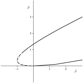
Let us stress that there are two allowed regions for the scale factor, one for $a\geq a_{m}=(\epsilon\rho_{0})^{1/3}>0$ and one for negative values of $a$. The effective pressure and energy density are

$$\tilde{\rho}=\frac{3+\varphi}{4\varphi^{2}}\rho=\frac{1-\epsilon\rho_{0}}{(1-{\epsilon}\rho)^{2}}\big{(}1-\hbox{$\frac{3}{4}$}\epsilon\rho_{0}-\hbox{$\frac{1}{4}$}\epsilon\rho\big{)}\rho,$$

$$\tilde{p}=\frac{1-\varphi}{4\varphi^{2}}\rho=\frac{\epsilon}{4}\frac{1-\epsilon\rho_{0}}{(1-\epsilon\rho)^{2}}(\rho-\rho_{0})\rho.$$

This corresponds to an effective EoS; see Fig. 1a.

Figure 1: a) Effective EoS $\tilde{p}(\tilde{\rho})$. (The dash line corresponds to a negative energy density $\rho$ for visible matter, which may be considered unphysical.) b) Scale factors $\tilde{a}(a)$. Dash line is standard GR.

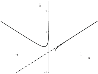
The relation between the scale factors is (see Fig. 1b)

$$\tilde{a}(a)=\sqrt{\frac{1-\epsilon\rho}{1-\epsilon\rho_{0}}}a.$$

At this point we can expand $\tilde{\rho}$ and $\tilde{p}$ as functions of $a$ and check that

$$\tilde{p}=-\left(\tilde{\rho}+\hbox{$\frac{1}{3}$}\hbox{$\frac{d\tilde{\rho}}{d\tilde{a}}$}\tilde{a}\right),\qquad\frac{d\tilde{\rho}}{d\tilde{a}}=\frac{d\tilde{\rho}}{d\rho}\frac{d\rho}{da}\frac{da}{d\tilde{a}}=-3\rho_{0}a^{-4}\frac{d\tilde{\rho}}{d\rho}\left(\frac{d\tilde{a}}{da}\right)^{-1}.$$ (4.1)

The condition (4.1) is in fact generally equivalent to conservation laws for the effective energy-momentum stress tensor $\tilde{T}_{\mu\nu}$, which is general follows from conservation of the original energy-momentum stress tensor $T_{\mu\nu}$ (see Appendix A), which in turn follows from EoS imposed for matter, or, equivalently, from covariance of the matter Lagrangian.

Then one decides what kind of effective matter is needed in the model. This is not something decided within cosmology, it can be a choice of ours or an input from other physics (e.g., constraints from baryogenesis or structures formation).

For example, let us assume we want a model with cosmological constant, dust and radiation. This corresponds to a total density in the form

$$\hat{\rho}(\tilde{a})=\tilde{\rho}{}_{\Lambda}^{0}+\frac{\tilde{\rho}{}^{0}_{d}}{\tilde{a}^{3}}+\frac{\tilde{\rho}{}^{0}_{r}}{\tilde{a}^{4}}$$

with the parameters $(\tilde{\rho}{}_{\Lambda}^{0},\tilde{\rho}{}^{0}_{d},\tilde{\rho}{}^{0}_{r})$ to be determined so that $\hat{\rho}$ best approximates $\tilde{\rho}$.

Best fit can be obtained simply by imposing that the value, first and second derivatives of $\tilde{\rho}$ and $\hat{\rho}$ coincides at $\tilde{a}=1$, i.e., today. The best approximation takes the form of

$$\tilde{\rho}{}_{\Lambda}^{0}=\tilde{\rho}{}_{\Lambda}^{0}(\epsilon,\rho_{0}),\qquad\tilde{\rho}{}^{0}_{d}=\tilde{\rho}{}^{0}_{d}(\epsilon,\rho_{0}),\qquad\tilde{\rho}{}^{0}_{r}=\tilde{\rho}{}^{0}_{r}(\epsilon,\rho_{0}).$$ (4.2)

This functions are quite complicated functions, also for a simple model as the one we are considering here. However, one can have an idea of their shape (and the effective physics they describe) by expanding them for small $\epsilon$ (i.e., small modification of standard GR). In this case we have:

$$\tilde{\rho}{}_{\Lambda}^{0}\simeq\frac{\rho_{0}^{2}}{8}\epsilon-\frac{\rho_{0}^{3}}{4}\epsilon^{2},\qquad\tilde{\rho}{}^{0}_{d}\simeq\rho_{0}-\frac{5\rho_{0}^{2}}{4}\epsilon+\frac{11\rho_{0}^{3}}{8}\epsilon^{2},\qquad\tilde{\rho}{}^{0}_{r}\simeq\frac{9\rho_{0}^{2}}{8}\epsilon-\frac{9\rho_{0}^{3}}{8}\epsilon^{2}.$$

Let us remark that those reduce to visible matter (dust only) for $\epsilon=0$ and that all energy densities are positive for a small positive $\epsilon$.

This means that Palatini $f({\cal R})$-cosmology with $f({\cal R})={\cal R}-\hbox{$\frac{\epsilon}{2}$}{\cal R}^{2}$ and purely dust visible matter is well approximated today by standard cosmology with cosmological constant, dust and radiation. Of course, far in the past and future the approximation fails to be accurate.

We can also compute the abundances of different kinds of effective matter by dividing by the critical density today $\tilde{\rho}_{0}^{\rm cr}=3\tilde{H}_{0}=\rho_{0}$ to obtain the effective abundance parameters today

$$\tilde{\Omega}{}_{\Lambda}^{0}\simeq\frac{\rho_{0}}{8}\epsilon-\frac{\rho_{0}^{2}}{4}\epsilon^{2},\qquad\tilde{\Omega}{}^{0}_{d}\simeq 1-\frac{5\rho_{0}}{4}\epsilon+\frac{11\rho_{0}^{2}}{8}\epsilon^{2},\qquad\tilde{\Omega}{}^{0}_{r}\simeq\frac{9\rho_{0}}{8}\epsilon-\frac{9\rho_{0}^{2}}{8}\epsilon^{2}.$$

In principle, one can try and determine $\epsilon$ so that, e.g., $\Omega_{\Lambda}\simeq 0.75$ as observed, e.g., by WMAP. However, there are numerical evidences that the (exact) abundance of effective dark energy in $f({\cal R})={\cal R}-\hbox{$\frac{\epsilon}{2}$}{\cal R}^{2}$ models cannot exceed a value of about 0.62. In this case the whole family of models $f({\cal R})={\cal R}-\hbox{$\frac{\epsilon}{2}$}{\cal R}^{2}$ can be rejected since it is not compatible with observations.

4.1 The model surface

What we got above as a description of the cosmological model is the abundance parameters $\big{(}\Omega^{0}_{k},\Omega^{0}_{\Lambda},\Omega^{0}_{d},\Omega^{0}_{r},\dots\big{)}$ as functions of the parameter $\epsilon$ which in fact parametrises the family of models under consideration, namely in the simple example of the function $f({\cal R})={\cal R}-\hbox{$\frac{\epsilon}{2}$}{\cal R}^{2}$.

Abundances are particularly interesting parameters since they can be measured quite directly observing the Cosmic Microwave Background radiation. Accordingly, one has independent effective abundances $\Omega^{0}_{i}$ ($i=1,\dots,n$) which result from observations (the curvature $\Omega^{0}_{k}$ is eliminated by the constraint $\sum\Omega_{i}^{0}=1$). More generally, a family of models is represented by a number of parameters $\epsilon^{\alpha}$ (the constants determining the function $f({\cal R})$) and the independent abundances

$$\Omega^{0}_{i}=\Omega^{0}_{i}(\epsilon^{\alpha})$$ (4.3)

define a map from the set of models into the space of cosmic pies.

By letting the parameters $\epsilon^{\alpha}$ vary, the equations (4.3) describe a parametrised subset $\Sigma\subset{\mathbb{R}}^{n}$. Each point on $\Sigma$ represents the predictions of a model in the family. In this setting one can translate physical issues in geometrical claims, e.g., whether an observed cosmic pie $(\Omega^{0}_{i})\in{\mathbb{R}}^{n}$ belongs to the image $\Sigma\subset{\mathbb{R}}^{n}$.

The subset $\Sigma$ is called the model surface and it captures all the predictions of the models in terms of observable quantities. Thus if the observed cosmic pie is not on $\Sigma$ then the family cannot account for observations and must be abandoned.

In the model above, one has one parameter $\epsilon$ and two independent abundances $\big{(}\Omega^{0}_{\Lambda},\Omega^{0}_{d}\big{)}\in{\mathbb{R}}^{2}$. The corresponding line representing the model is shown in Fig. 2.

Figure 2: Line model for $f({\cal R})={\cal R}-\hbox{$\frac{\epsilon}{2}$}{\cal R}^{2}$. Dash line is the constraint $\sum_{i}\Omega^{0}_{i}=1$. The dot is the observered cosmic pie (e.g., WMAP).

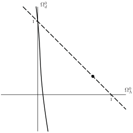
Since observations are considered to support $\big{(}\Omega^{0}_{\Lambda},\Omega^{0}_{d}\big{)}\simeq(0.75,0.25)$ the family is discarded.

More generally, one can consider further observable quantities as the cosmographic parameters

$$q=-\frac{1}{H^{2}}\frac{\ddot{a}}{a},\qquad j=\frac{1}{H^{3}}\frac{\dot{\ddot{a}}}{a},\qquad j=\frac{1}{H^{4}}\frac{\ddot{\ddot{a}}}{a},\qquad\dots$$

in the target space. On the other hand, ideally, one can expand the function $f({\cal R})$ in series (for example in Laurent series) and consider the infinitely many coefficients as the family parameters $\epsilon^{\alpha}$. Although, this becomes mathematically elaborated (having an infinite-dimensional surface embedded into an infinite-dimensional space) one can regard this as a universal setting to represent theories and observations as geometric intrinsic claims even when one may simplify it projecting to finite-dimensional representations in some particular context. For example, in this context is relatively easy and clear to argue if relations among observables hold in general or are valid within a specific family of theories when they emerge on the surface.

5 Conclusions and perspectives

In the literature, Palatini $f({\cal R})$-theories have not been studied much because of a number of shortcomings they are believed to have; see, for example, [8] and [25] where it was noticed that Palatini variation is not generally equivalent to metric variation. Since we totally agree on this point, we did not consider metric variations which are different theories. For us Palatini theories are motivated by the EPS formalism and they are, in our opinion, more natural than the metric ones.

In the second place, one can perform a conformal on-shell transformation to show dynamical equivalence with purely metric Brans–Dicke theories (with a suitable potential); see [12, 15]. Since Brans–Dicke models (without a potential) are ruled out by solar system observations (e.g., precession of Mercury’s perihelia) it has been claimed that then any Palatini $f({\cal R})$-theory should be ruled out as well. This is false due to two issues. First, one should consider the role of the potential. Second, and more importantly, although field equations of the two theories are equivalent that does not imply a complete physical equivalence. In particular, in the case of precession of perihelia, the test on Brans–Dicke models is performed by assuming that planets go along timelike geodesics of $g$ while in Palatini $f({\cal R})$-theories they go along geodesics of $\tilde{g}$. One can show by a detailed analysis that there is a huge family of Palatini $f({\cal R})$-theories which in fact pass the test of perihelia; see [19].

Moreover, the conformal transformation needed to recast Palatini-$f({\cal R})$ theories into Brans–Dicke form is quite peculiar. One starts with a Palatini theory in which conformal transformations act on the metric (which do not touch the connection which is independent) and they are symmetries. Then one solves the field equation related to the connection learning that the connection is in fact the Levi-Civita connection of a suitably defined conformal metric $\tilde{g}$. One is left with the field equation depending on the metric (and the conformal factor) alone since the connection has been eliminated. At this point by performing the inverse conformal transformation on the metric (which now affects the connection as well) the theory is recast into a Brans–Dicke form. There should be no surprise that the two theories are inequivalent since the latter transformation is not a symmetry.

Another, issue is about star models. It was argued that assuming polytropic equation of state (EoS) one cannot match the inner solution with the outer solution for $g$. This is in fact true due to the fact that the conformal factor is continuous but not ${\cal C}^{1}$ on the surface of the star. If one matches the conformal metric $\tilde{g}$ (how is natural to do in view of the interpretation above) this is possible and the discontinuity appears only in the original metric $g$. Moreover, it has been noted that here the issue is due to the assumption about the EoS which is not a fundamental principle. Allowing a slight deformation of EoS one can in fact match the metrics at the surface of the star. The same result can be obtained by changing the external solution from a vacuum solution to an almost-vacuum one as it is reasonable and physically sound; see [3, 20, 21].

We showed how to classify extended cosmological models with respect to their predictions about the cosmic pie observations and to their predictions of the evolution of the scale factor.

We showed that, the species revealed in the cosmic pie are essentially a choice in cosmology, or, in other words, an input from other physics (structure formation, baryogenesis, …). However, once this input is given, extended gravity models produce quantitative predictions which allow in principle to falsify or corroborate models.

The choice of effective species is not forced by mathematics essentially because of the approximation method used. We chose to expand $\tilde{\rho}$ in negative powers of $\tilde{a}$ around the value $\tilde{a}=1$. Even if we had $\tilde{\rho}=3\tilde{a}^{-2}$ and decide we want to see only dust and cosmological factor we would find

$$\tilde{\rho}\sim 1+\frac{2}{{\tilde{a}}{}^{3}},$$

which approximates the actual effective density around today $\tilde{a}=1$.

One clearly sees that if one has a direct observation of $a(t)$ in the past and assumes the approximated value then one can predict at what time in the past the deviation is first observed.

Let us stress that, although it may not be computationally simple, the predictions of the models for the cosmic pie are extracted before solving the model.

Figure 3: Approximation of a curvature density by cosmological constant and dust (dash line is the approximated density).

Future investigations are to be devoted to models in which the conformal factor stays positive everywhere, so that signature changes are prevented.

Another research perspective will be investigating how one can encode physical properties (e.g., late time acceleration) as properties of the model surface and viceversa reading physical properties of the theories from the geometry of the surface. Currently, the main difficulty to be overcome is to control with enough generality the inversion of the master equation which plays a prominent role in expressing the embedding map (4.2). On the other hand, the model surface may be a good tool exactly because it shows that the properties are algebraically encoded in the model precisely through the master equation of the theory.

Appendix A Conservation laws

In a $f({\cal R})$-theory, the effective stress tensor $\tilde{T}_{\mu\nu}$ is defined by equation (2.2). Its conservation with respect to the conformal metric $\tilde{g}$ reads as $\tilde{\nabla}_{\mu}\tilde{T}^{\mu\nu}=0$, where indices have been raised by $\tilde{g}$. The relations between controvariant stress tensors is then

$$\varphi^{3}\tilde{T}^{\mu\nu}=T^{\mu\nu}-(\varphi{\cal R}-f({\cal R}))g^{\mu\nu}.$$

Let us stress that indices of $\tilde{T}^{\mu\nu}$ are here raised by $\tilde{g}$, while indices of $T^{\mu\nu}$ are raised by $g$.

Let us introduce the tensor

$$K^{\alpha}_{\beta\mu}=\{\tilde{g}\}^{\alpha}_{\beta\mu}-\{g\}^{\alpha}_{\beta\mu}=-\hbox{$\frac{1}{2}$}\big{(}g^{\alpha\epsilon}g_{\beta\mu}-2\delta^{\alpha}_{(\beta}\delta^{\epsilon}_{\mu)}\big{)}{\buildrel\ast\over{\nabla}}_{\epsilon}\ln\varphi,$$

which accounts for the difference between the connections of the metrics $\tilde{g}$ and $g$. Hereafter the covariant derivatives with respect to $g$ will be denoted by $\nabla_{\epsilon}$ while the ones with respect to $\tilde{g}$ will be denoted by $\tilde{\nabla}_{\epsilon}$. The symbol ${\buildrel\ast\over{\nabla}}_{\epsilon}$ means a covariant derivative when it is independent of any connection (in this case being applied to the scalar $\ln\varphi$).

One can easily show that

$$K^{\mu}_{\epsilon\mu}\tilde{T}^{\epsilon\nu}=2\tilde{T}^{\epsilon\nu}{\buildrel\ast\over{\nabla}}_{\epsilon}\ln\varphi$$

and

$$K^{\nu}_{\epsilon\mu}\tilde{T}^{\epsilon\mu}=\tilde{T}^{\nu\epsilon}{\buildrel\ast\over{\nabla}}_{\epsilon}\ln\varphi-\hbox{$\frac{1}{2}$}g^{\nu\alpha}g_{\epsilon\mu}\tilde{T}^{\epsilon\mu}{\buildrel\ast\over{\nabla}}_{\epsilon}\ln\varphi.$$

Then one has directly that

$$\varphi^{3}\tilde{\nabla}_{\mu}\tilde{T}^{\mu\nu}=\varphi^{3}\big{(}\nabla_{\mu}\tilde{T}^{\mu\nu}+K^{\mu}_{\epsilon\mu}\tilde{T}^{\epsilon\nu}+K^{\nu}_{\epsilon\mu}\tilde{T}^{\epsilon\mu}\big{)}$$

$$\hphantom{\varphi^{3}\tilde{\nabla}_{\mu}\tilde{T}^{\mu\nu}}{}=\nabla_{\mu}T^{\mu\nu}-\hbox{$\frac{1}{2}$}g^{\nu\alpha}{\buildrel\ast\over{\nabla}}_{\alpha}\ln\varphi\big{(}T^{\mu\epsilon}-f({\cal R})g^{\mu\epsilon}\!-\hbox{$\frac{1}{2}$}Tg^{\mu\epsilon}\big{)}g_{\mu\epsilon}-g^{\nu\alpha}{\buildrel\ast\over{\nabla}}_{\alpha}f({\cal R})-\hbox{$\frac{1}{2}$}g^{\nu\alpha}{\buildrel\ast\over{\nabla}}_{\alpha}T$$

$$\hphantom{\varphi^{3}\tilde{\nabla}_{\mu}\tilde{T}^{\mu\nu}}{}=\nabla_{\mu}T^{\mu\nu}+g^{\nu\alpha}\big{(}f^{\prime\prime}({\cal R}){\cal R}{\buildrel\ast\over{\nabla}}_{\alpha}{\cal R}-f^{\prime}({\cal R}){\buildrel\ast\over{\nabla}}_{\alpha}{\cal R}-\hbox{$\frac{1}{2}$}{\buildrel\ast\over{\nabla}}_{\alpha}T\big{)}.$$

However, by taking the covariant derivative of the master equation (2.1) one has

$$f^{\prime\prime}({\cal R}){\cal R}{\buildrel\ast\over{\nabla}}_{\alpha}{\cal R}+f^{\prime}({\cal R}){\buildrel\ast\over{\nabla}}_{\alpha}{\cal R}-2f^{\prime}({\cal R}){\buildrel\ast\over{\nabla}}_{\alpha}{\cal R}=\hbox{$\frac{1}{2}$}{\buildrel\ast\over{\nabla}}_{\alpha}T,$$

so that one simply has

$$\varphi^{3}\tilde{\nabla}_{\mu}\tilde{T}^{\mu\nu}=\nabla_{\mu}T^{\mu\nu},$$

so that $\tilde{T}^{\mu\nu}$ is conserved with respect to $\tilde{g}$ iff $T^{\mu\nu}$ is conserved with respect to $g$.

Appendix B Model solution

Solving the FRW equations may be difficult though in a sense trivial since, in the end, one has to solve the Weierstrass equations with

$$\tilde{\Phi}(\tilde{a})=-k+\frac{1}{3}\tilde{\rho}(a(\tilde{a}))\tilde{a}^{2},$$

i.e., computing the integral

$$\tilde{t}=\tilde{t}_{0}+\int_{\tilde{a}_{0}}^{\tilde{a}}\frac{d\tilde{a}}{\sqrt{\tilde{\Phi}(\tilde{a})}}.$$

Maple can make it (with some effort) numerically (which means one can obtain a plot of $\tilde{a}=\tilde{a}(\tilde{t})$).

An easier way is to change variable back to $(t,a)$, solve the equation and then compute the conformal factor, the new time and the conformal scale factor. This can be done by considering that

$$\frac{d\tilde{a}}{d\tilde{t}}=\frac{d\tilde{a}}{da}\frac{da}{dt}\frac{dt}{d\tilde{t}}\qquad\Rightarrow\qquad\left(\frac{da}{dt}\right)^{2}=\left({\frac{d\tilde{t}}{dt}}\right)^{2}\left({\frac{d\tilde{a}}{da}}\right)^{-2}\tilde{\Phi}(\tilde{a})=:\Phi(a).$$

Since we know that $d\tilde{t}=\sqrt{\varphi}dt$ and $\tilde{a}(a)=a\sqrt{\varphi}$ one has for $f({\cal R})={\cal R}-\hbox{$\frac{\epsilon}{2}$}{\cal R}^{2}$

$$\Phi(a):=\left(\frac{3-\epsilon\rho(a)}{3-\epsilon\rho_{0}}\right)\left({\frac{d\tilde{a}}{da}(a)}\right)^{-2}\tilde{\Phi}(\tilde{\rho}(a)).$$

Once we have $\Phi(a)$ we obtain the time coordinate as

$$t(a)=t_{0}+\int_{a_{0}}^{a}\frac{da}{\sqrt{\Phi(a)}}$$

and the conformal time as

$$\tilde{t}(a)=\tilde{t}_{0}+\int_{t_{0}}^{t}\sqrt{\varphi(a(t))}dt=\tilde{t}_{0}+\int_{a_{0}}^{a}\sqrt{\varphi(a)}\frac{da}{\sqrt{\Phi(a)}}.$$

Finally the original density $\rho$ is given as $\rho(a)$ by EoS as well as the conformal density and pressure $(\tilde{\rho}(a),\tilde{p}(a))$.

Figure 4: Weierstrass function $\Phi(a)$. (Dash line is standard GR.)

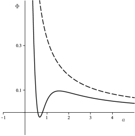
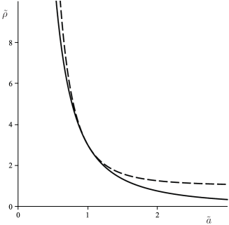
In our special case $f({\cal R})={\cal R}-\hbox{$\frac{\epsilon}{2}$}{\cal R}^{2}$, setting $\epsilon=\hbox{$\frac{1}{2}$}$ and $\rho_{0}=1$ , one obtains (see Fig. 4)

$$\Phi(a)=\frac{1}{3a}\frac{(2a^{3}-1)(5a^{3}-1)}{(4a^{3}+1)^{2}}$$

with two allowed regions, one being $a\in[0,5^{-1/3}]$ the other being $a\geq 2^{-1/3}$. The first region corresponds to an oscillating behaviour, hence to a closed universe. The second region corresponds to an expanding universe. Let us consider the second region.

Figure 5: a) Scale factor $a$ as a function of $t$ (dash line standard GR). b) Energy density $\rho$ for visible matter as a function of $t$ (dash line standard GR).

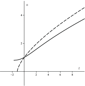
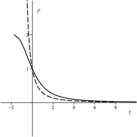
The original scale factor hence appears as a quite natural parameter to (more) easily integrate equations for $\tilde{a}$.

In this way one is able to plot parametrically everything; see Fig. 5. Notice how the energy density of the visible matter $\rho(t)$ stays bounded and the scale factor $a(t)$ stays non-zero when standard GR has a singularity.

This means that the solution can be extended to negative $t$ and the big bang singularity is avoided (as some model of quantum gravity predicts; see [6]).

Acknowledgements

We are grateful to A. Borowiec for comments and discussion. We acknowledge the contribution of INFN (Iniziativa Specifica QGSKY), the local research project Metodi Geometrici in Fisica Matematica e Applicazioni (2015) of Dipartimento di Matematica of University of Torino (Italy). This paper is also supported by INdAM-GNFM.

References

- [1] Allemandi G., Borowiec A., Francaviglia M., Accelerated cosmological models in first-order nonlinear gravity, Phys. Rev. D 70 (2004), 043524, 11 pages, hep-th/0403264.
- [2] Allemandi G., Borowiec A., Francaviglia M., Accelerated cosmological models in Ricci squared gravity, Phys. Rev. D 70 (2004), 103503, 13 pages, hep-th/0407090.
- [3] Barausse E., Sotiriou T.P., Miller J.C., A no-go theorem for polytropic spheres in Palatini gravity, Classical Quantum Gravity 25 (2008), 062001, 7 pages, gr-qc/0703132.
- [4] Barreto A.B., Almeida T.S., Romero C., Extending the ADM formalism to Weyl geometry, AIP Conf. Proc. 1647 (2015), 89–93, arXiv:1503.08455.
- [5] Benenti S., Rational cosmology, in preparation.
- [6] Bojowald M., Loop quantum cosmology, Living Rev. Relativ. 11 (2008), 4, 131 pages, gr-qc/0601085.
- [7] Borowiec A., Kamionka M., Kurek A., Szydlowski M., Cosmic acceleration from modified gravity with Palatini formalism, J. Cosmol. Astropart. Phys. 2012 (2012), no. 2, 027, 32 pages, arXiv:1109.3420.
- [8] Buchdahl H.A., Quadratic Lagrangians and Palatini’s device, J. Phys. A: Math. Gen. 12 (1979), 1229–1234.
- [9] Capozziello S., Curvature quintessence, Internat. J. Modern Phys. D 11 (2002), 483–491, gr-qc/0201033.
- [10] Capozziello S., De Laurentis M., Extended theories of gravity, Phys. Rep. 509 (2011), 167–320, arXiv:1108.6266.
- [11] Capozziello S., Francaviglia M., Extended theories of gravity and their cosmological and astrophysical applications, Gen. Relativity Gravitation 40 (2008), 357–420, arXiv:0706.1146.
- [12] De Felice A., Tsujikawa S., theories, Living Rev. Relativ. 13 (2010), 3, 161 pages, arXiv:1002.4928.
- [13] Di Mauro M., Fatibene L., Ferraris M., Francaviglia M., Further extended theories of gravitation: Part I, Int. J. Geom. Methods Mod. Phys. 7 (2010), 887–898, arXiv:0911.2841.
- [14] Ehlers J., Pirani F.A.E., Schild A., The geometry of free fall and light propagation, in General Relativity (Papers in Honour of J.L. Synge), Clarendon Press, Oxford, 1972, 63–84.
- [15] Faraoni V., gravity: successes and challenges, arXiv:0810.2602.
- [16] Fatibene L., Ferraris M., Francaviglia M., Mercadante S., Further extended theories of gravitation: Part II, Int. J. Geom. Methods Mod. Phys. 7 (2010), 899–906, arXiv:0911.2842.
- [17] Fatibene L., Garruto S., Polistina M., Breaking the conformal gauge by fixing time protocols, Int. J. Geom. Methods Mod. Phys. 12 (2015), 1550044, 14 pages, arXiv:1410.1284.
- [18] Fatibene L., Francaviglia M., From the Ehlers–Pirani–Schild analysis on the foundations of gravitational theories to extended theories of gravity and dark matter, PoS Proc. Sci. (2011), PoS(CORFU2011), 054, 16 pages.
- [19] Fatibene L., Francaviglia M., Mathematical equivalence versus physical equivalence between extended theories of gravitations, Int. J. Geom. Methods Mod. Phys. 11 (2014), 1450008, 21 pages, arXiv:1302.2938.
- [20] Mana A., Fatibene L., Ferraris M., A further study on Palatini -theories for polytropic stars, J. Cosmol. Astropart. Phys. 2015 (2015), no. 10, 040, 19 pages, arXiv:1505.06575.
- [21] Olmo G.J., Hydrogen atom in Palatini theories of gravity, Phys. Rev. D 77 (2008), 084021, 8 pages, arXiv:0802.4038.
- [22] Olmo G.J., Singh P., Covariant effective action for loop quantum cosmology à la Palatini, J. Cosmol. Astropart. Phys. 2009 (2009), no. 1, 030, 10 pages, arXiv:0806.2783.
- [23] Perlick V., Characterization of standard clocks by means of light rays and freely falling particles, Gen. Relativity Gravitation 19 (1987), 1059–1073.
- [24] Poulis F.P., Salim J.M., Weyl geometry and gauge-invariant gravitation, Internat. J. Modern Phys. D 23 (2014), 1450091, 24 pages, arXiv:1305.6830.
- [25] Querella L., Variational principles and cosmological models in higher-order gravity, Ph.D. thesis, Université de Liegè, 1998, gr-qc/9902044.
- [26] Romero C., Fonseca-Neto J.B., Pucheu M.L., General relativity and Weyl geometry, Classical Quantum Gravity 29 (2012), 155015, 18 pages, arXiv:1201.1469.
- [27] Salim J.M., Sautú S.L., Gravitational theory in Weyl integrable spacetime, Classical Quantum Gravity 13 (1996), 353–360.
- [28] Weyl H., Gravitation und Elektrizität, Monatsbericht Kön.-Preuss. Akad. Wiss. Berlin (1918), 465–480.