Vanderbilt University Center for Multiscale Modeling and Simulation (MuMS), Nashville, TN 37235 Vanderbilt University Center for Multiscale Modeling and Simulation (MuMS), Nashville, TN 37235 Vanderbilt University Center for Multiscale Modeling and Simulation (MuMS), Nashville, TN 37235 Department of Chemistry, Vanderbilt University, Nashville, TN 37235

Development of a coarse-grained water forcefield via multistate iterative Boltzmann inversion

1 Introduction

Coarse-grained (CG) models have proven to be useful in many fields of chemical research ^{1, 2, 3, 4, 5, 6, 7, 8, 9, 10}, allowing molecular simulation to be performed on larger system sizes and access longer timescales than is possible with atomistic-level models, enabling complex phenomena such as hierarchical self-assembly to be described. ^{11, 12} In CG simulations of aqueous systems, especially ones with significant amounts of hydrophobic and/or hydrophilic interactions, the water model is important and can have a major impact on the resulting properties of the system.¹³

While the assignment of atoms to CG beads (i.e., defining the CG mapping) is relatively straightforward for most chemical systems (e.g., aggregating four methyl groups bonded in sequence into a single CG bead), mapping an atomistic water trajectory to the CG level (i.e., grouping several water molecules into a single CG bead) is not as well-defined given the lack of permanent bonds between water molecules. This ambiguity presents a problem for structure-based methods that require an atomistic configuration to be mapped to the corresponding CG configuration, e.g., to generate target radial distribution functions (RDFs) against which the forcefield is optimized. As such, the majority of many-to-one CG models of water (i.e., where one CG bead represents multiple water molecules) have instead been derived by assuming a functional form of the forcefield and optimizing the associated parameters to match selected physical properties of water, such as density, vaporization enthalpy, surface tension, etc.^{13, 14, 15, 16, 17, 18, 19} For example, Chiu et al. developed a 4:1 CG water forcefield by optimizing the parameters of a Morse potential to accurately reproduce the surface tension and density of liquid water.¹⁸ Despite capturing the interfacial properties and density, this potential overestimates structural correlations, as one might expect given that structural data was not used in the optimization.

Recently, Hadley and McCabe²⁰ proposed a method for mapping configurations of atomistic water to their CG representations using the $k$-means clustering algorithm. Subsequently in related work, van Hoof et al.²¹ developed the CUMULUS method for mapping atoms to CG beads. Both methods enable dynamic mapping of multiple water molecules to a single CG bead, allowing structure-based schemes to be used. Here, dynamic refers to a CG mapping that changes over the course of the atomistic trajectory, i.e., different water molecules are assigned to different CG beads in each frame of the atomistic trajectory. Both works employed the iterative Boltzmann inversion (IBI)²² method to derive the intermolecular interactions by optimizing a numerical, rather than analytical, potential to reproduce RDFs calculated from the atomistic-to-CG mapped configurations.^{21, 20} The forcefields derived are similar and show good agreement with the structural properties and density of the atomistic water models studied. However, neither model is able to accurately reproduce interfacial properties, since they were derived solely from bulk fluid data. This failure to capture the interfacial properties is a consequence of the single-state nature of the IBI approach, and may alter the balance of hydrophobic and hydrophilic interactions when using these water models in multicomponent systems.

Recently, the multistate IBI (MS IBI) method was developed as an extension of the original IBI approach,²³ with the goal of reducing state dependence and structural artifacts often found in IBI-based potentials. ^{24, 25, 26} A significant issue related to the IBI method is that a multitude of potentials may give rise to similar RDFs, and the method cannot necessarily differentiate which of the many potentials is most accurate, as only RDF matching is considered. MS IBI operates based on the idea that different thermodynamic states will occupy different regions of potential “phase space” (i.e., regions where potentials give rise to similar RDFs), and that the most transferable, and thus most accurate, potential lies in the overlap of phase space for the different states. That is, by optimizing a potential simultaneously against multiple thermodynamic states, MS IBI provides constraints to the optimization, forcing the method to derive potentials that exist in this overlap region, and thus are transferable among the states considered. The MS IBI approach has been shown to reduce state dependence and improve the quality of the derived potentials, as compared to the original IBI method.²³

In this work, multistate iterative Boltzmann inversion (MS IBI) is used to derive an intermolecular potential that captures both bulk and interfacial properties of water, improving upon the CG water model of Hadley and McCabe.²⁰ Again, optimizations are carried out using the MS IBI method, where both bulk and interfacial systems are used simultaneously as target conditions for the optimization. MS IBI is also used, for the first time, in a multi-ensemble context, enabling optimizations in both the canonical (NVT) and isothermal-isobaric (NPT) ensembles to be performed simultaneously to derive the density-pressure relationship of the system. To further constrain the optimization, a slightly modified version of the Chiu et al. CG water forcefield, optimized for surface tension, is used as a starting condition, allowing the MS IBI method to make specific modifications to the potential to improve structural properties. The remainder of the paper is organized as follows: In Methods, a brief overview of the $k$-means clustering and MS IBI algorithms is given and the models used are described. The potential derivation is then presented, validated, and compared to existing CG water models in the Results section and finally, conclusions are drawn about the applicability of the derived CG model and the broader applicability of the MS IBI method discussed.

2 Methods

2.1 $k$-means Clustering Algorithm

Mapping a water trajectory to the CG level is inherently different than mapping a larger molecule’s trajectory, since for water, atoms mapped to a single CG bead exist on different molecules. Furthermore, the water molecules mapped to a common bead are not likely to remain associated throughout the full simulation because of thermal diffusion. A dynamic mapping scheme is therefore required for water. Following the work of Hadley and McCabe,²⁰ the $k$-means algorithm is used to map the atomistic water trajectory to the CG level. In short, $k$-means is a clustering algorithm that is used to find clusters of data points in a large data set. The positions of the water molecules are here analogous to the points in the data set and waters mapped to a single bead are analogous to the clusters. More details of the algorithm can be found elsewhere.^{20, 27} While the $k$-means algorithm can be used to group together any number of water molecules, a 4:1 mapping is chosen, as this was found in prior to provide the best balance between accuracy and computational efficiency,²⁰ and 4:1 models are common in the literature.^{17, 18, 20}

2.2 Multistate Iterative Boltzmann Inversion Method

MS IBI was used to derive the intermolecular potential between water beads. The goal of MS IBI is to derive a single potential that can be used over a range of thermodynamic states. As an extension of the original IBI method,²² the potential is updated based on the average differences in CG and target RDFs at multiple states (i.e., a single potential for each pair is updated based on RDFs from multiple states). The potential is adjusted according to

$$V_{i+1}(r)=V_{i}(r)-\frac{1}{N}\sum_{s}\alpha_{s}(r)k_{B}T_{s}\ln\left[\frac{g^{*}_{s}(r)}{g^{i}_{s}(r)}\right],$$ (1)

where $V_{i}(r)$ is the pair potential as a function of separation $r$ at the $i^{th}$ iteration; $N$ the number of target states; $\alpha(r)$ an effective weighting factor for each state, allowing more or less emphasis to be put on a particular target state; $k_{B}$ the Boltzmann constant and $T$ the absolute temperature; $g^{i}_{s}(r)$ the RDF from the CG simulation at iteration $i$ and state $s$; $g^{*}_{s}(r)$ the target RDF at state $s$. $\alpha_{s}(r)$ was chosen to be a linear function of the form

$$\alpha_{s}(r)=\alpha_{0,s}(1-r/r_{cut})$$ (2)

such that $\alpha(r_{cut})=0$, and the potential remains 0 for $r\geq r_{cut}$. This form of $\alpha(r)$ also places more emphasis on the short-ranged part of the potential to suppress long-range structural artifacts.

An initial CG potential is assumed for each pair interaction. In theory, there are no restrictions on the initial potential, so it may take any form; however, in practice, the initial potential is often the potential of mean force (PMF) calculated from the Boltzmann inverted RDF. In this work, rather than taking an average of the PMFs over the states used, the initial potential used was slightly modified from the water model of Chiu et al., as discussed below.

A CG simulation is then run with the initial potential. Based on the RDFs from the CG simulation, the potential is updated according to Equation 1. The updated potential is used as input to the next cycle, and the process is repeated until some stopping criterion is met. Here, the stopping criterion is determined using the following fitness function

$$f_{fit}=1-\frac{\int_{0}^{r_{cut}}\mathrm{d}r\left|g^{i}(r)-g^{*}(r)\right|}{\int_{0}^{r_{cut}}\mathrm{d}r\left|g^{i}(r)\right|+\left|g^{*}(r)\right|}$$ (3)

where the optimization is stopped when the value of $f_{fit}$ exceeds a specified value (i.e., meets some tolerance), given below.

2.3 Models

Atomistic simulations of pure water were performed with the TIP3P model.²⁸ All atomistic systems contained 5,832 water molecules and were simulated in LAMMPS^{29, 30} using a 1 fs timestep. A cutoff distance of 12 Å was used for the van der Waals interactions; long-range electrostatics were handled with the PPPM method with a 12 Å real space cutoff. Three distinct states were simulated: bulk, NVT at 1.0 g/mL and 305 K; bulk, NPT at 305 K and 1.0 atm; and an NVT droplet state at 305 K, where the box from the bulk NVT state was expanded by a factor of 3 in one direction. Each atomistic simulation was run for 7 ns. The atomistic trajectories were mapped to the CG level using the $k$-means algorithm. Target RDFs were calculated from the final 5 ns of the mapped trajectory from each state (bulk NVT, bulk NPT, and droplet NVT). MS IBI was performed using the target data from each of the three states. The initial guess of the potential is given as a Morse potential of the form

$$V(r)=D_{e}\left(e^{-2\beta(r-r_{eq})}-2e^{-\beta(r-r_{eq})}\right)$$ (4)

where $r_{eq}$ is the location of the potential minimum, $-D_{e}$ is the value of the potential minimum, and $\beta$ is related to the width of the potential well. Parameters are taken to be those from Chiu et al.: $D_{e}=0.813$ kcal/mol, $\beta=0.556$ Å${}^{-}1$, and $r_{eq}=6.29$ Å, however, we note that the potential was adjusted so that $\beta=0.5$ Å^-1 for $r<r_{eq}$. This change was made to increase sampling as small separations, because numerical issues arise in the potential update when the CG RDF is zero but the target RDF is nonzero. This modification of the potential will slightly alter the properties as compared to the original model, as discussed below. The potential update scaling factor $\alpha_{0,s}$ (see Equations 1 and 2) was set to 0.7 to avoid large updates to the potential. The optimizations were stopped when $f_{fit}\geq 0.98$ for each state and $f_{fit}(i)-f_{fit}(i-1)<0.001$.

All optimizations were performed with the open-source MSIBI Python package we developed,³¹ which calls HOOMD-Blue^{32, 33, 34} to run the CG simulations and uses MDTraj^{35, 36} for RDF calculations and file-handling. CG simulations were run at the same states as the atomistic systems. Initial CG configurations were generated from the CG-mapped atomistic trajectories at each state. As a result of the 4:1 mapping, CG water simulations contained 1,458 water beads. All CG simulations were run with a 10 fs timestep. The derived CG potential was set to 0 beyond the cutoff of 12 Å.

The surface tension $\gamma$ of the droplet state was calculated as

$$\gamma=\frac{1}{2}L_{z}\left<P_{zz}-\frac{P_{xx}+P_{yy}}{2}\right>,$$ (5)

where $L_{z}$ is the length of the box in the expanded direction, $P_{zz}$ is the pressure component in the direction normal to the liquid-vapor interfaces, $P_{xx}$ and $P_{yy}$ are the pressure components in the directions lateral to the interfaces, and the angle brackets denote a time average. The factor of $1/2$ is included to account for the two interfaces that are present in the droplet simulation setup.

3 Results and Discussion

3.1 Modified Chiu Potential

We first consider the impact of modifying the Chiu et al. potential to create a softer repulsion. Figure 1 plots the RDFs of the three target states for the original and modified potentials and the RDF of the 4:1 mapped state (i.e, the target data used later for the MS IBI optimization). The peak location of the NVT state is relatively unchanged; however, upon modification, there is a slight shift in the first peak for the NPT and interfacial states, allowing the model to access smaller separations, as was intended. The softer potential allows closer contact and thus allows the MS IBI algorithm to modify this region of the potential where the 4:1 mapped atomistic water has non-zero values of the RDF. The density predicted with both potentials is the same (0.991 $\pm$ 0.003 g/mL), however, due to the softening of the potential, the calculated surface tension of the droplet changes from 70.3 mN/m to 45 mN/m after the modification, although we note this value is still sufficient for the droplet to maintain a stable interface.

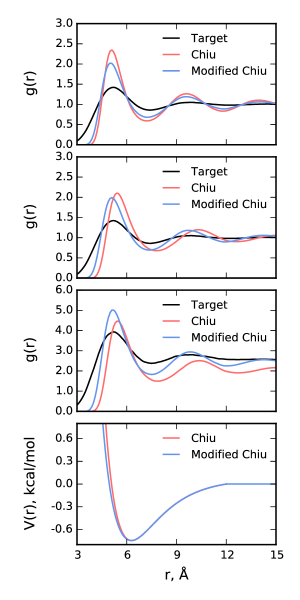
Figure 1: RDFs from simulations using the original and modified Chiu potentials. Top: NVT; middle: NPT; bottom-middle: interface; bottom: comparison of the two potentials.

3.2 Potential Derivation and Validation of Bulk Water

Starting from the modified Morse potential of Chiu et al., the new water forcefield is optimized using the bulk NVT and NPT states and the interfacial state. The results of the potential derivation are summarized in Figure 2, where it is clear that the modified Chiu et al. potentials (i.e., step 0) overestimates the structural correlations, as was also seen in Figure 1 for both the modified and original potentials. After only a few iterations, the RDFs match the targets with a high degree of accuracy. This trend is shown in Figure 3, which plots the fitness value from Equation 3 as a function of iteration. The value of $f_{fit}$ changes most rapidly in the first 3 steps of the optimization. After 10 iterations, the stopping criteria are met and the optimization stopped. While the changes to the potential are small, there is a noticeable shift in the location of the minimum to a slightly larger $r$ value and the potential becomes slightly more attractive. Although the shape of the attractive well is mostly unchanged, the potential more rapidly decays to 0 than the original Morse potential at larger $r$ values, while the shape of the repulsive regime at small $r$ is changed slightly. These subtle changes to the potential are sufficient to create significant changes in the RDF and provide excellent convergence of the structural correlations. Note that in Figure 1 and 2 the RDFs from the interfacial state do not decay to 1 at large $r$. This is due to the fact that 2/3 of the box is essentially devoid of particles, but the RDF is normalized based on the volume of the whole simulation box. This has no effect on the potential update scheme, as both the target and CG RDFs are normalized by the same factor, which cancels out in Equation 1.

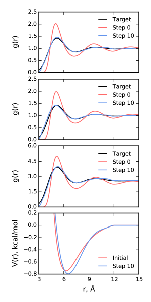
Figure 2: RDFs and potentials from the MS IBI potential derivation. Top: NVT; middle-top: NPT; middle-bottom: interface; bottom: potentials. The initial potential shows significant structural correlations missing from the target data. The derived potential at ten iterations shows excellent structural agreement with the target.

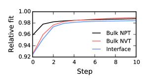
Figure 3: $f_{fit}$ from Equation 3 as a function of iteration in the potential derivation. Convergence with the criterion is found after 10 iterations.

In addition to accurately capturing the RDFs, the multi-ensemble approach provides an accurate estimate of the density at 305 K and 1 atm. NPT simulations performed using the optimized CG forcefield find a density of 1.027 $\pm$ 0.006 g/mL, compared to 1.037 $\pm$0.004 g/mL for TIP3P water. This approach is successful because the RDFs will not match if the pressure-density relationship is not satisfied, as the density is implicitly represented in Equation 1 through the RDF terms (i.e., the RDFs at the NPT state will not match the target RDFs if the density is significantly different than the density of the target state). In contrast, the original IBI method proposed the use of a pressure correction term of the form $\Delta V(r)=A(1-r/r_{cut})$ to account for the pressure.²² This approach has been successful, but requires a somewhat arbitrary estimate of the parameter $A$. While a method exists for estimating $A$ based on the virial expression,³⁷ some degree of trial-and-error is still necessary. Furthermore, the multi-ensemble approach within MS IBI does not require direct calculation of the pressure, which often demonstrates considerable fluctuations, providing a simpler route to account for the pressure in the CG model.

Calculation of the surface tension of the derived MS IBI potential yields a value of 42 mN/m, lower than the original Chiu et al. potential which was optimized to match experiment, but only slight perturbed from the modified potential (45 mN/m). This reduction is surface tension appears directly related to the softening of the potential, although, we note that this softening is required to provide an accurate match of the structure.

3.3 Validation and Comparison to Other Models

To further explore the efficacy of the MS IBI-derived model, comparisons are made to other CG water models in the literature, namely, the $k$-means based potential of Hadley and McCabe²⁰ derived via the single state (SS) IBI procedure (here referred to as the SS IBI potential) and the MARTINI potential.¹⁷ These models were chosen because they are short-ranged, non-polarizable, and 4:1 models. For reference, these potentials are plotted in Figure 4. Note that the MS IBI and SS IBI potentials are numerical (as they were derived via IBI), while the MARTINI potential is represented by a 12-6 Lennard-Jones potential with a well depth of 1.195 kcal/mol located at a separation of 5.276 Å. Note that all of the potentials considered in this paper provide a close estimate of the density of water at 1 atm and 305 K, as reported in Table 1.

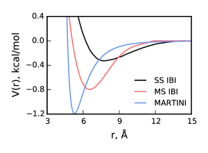
Figure 4: Interaction potentials from the CG water models compared in this work. The MS IBI and SS IBI potentials are numerical, derived with structure-based methods. MARTINI is a Lennard-Jones 12-6 potential.

Table 1: Density of CG water at 305 K, 1 atm with various models.

Model	$\rho$, g/mL
TIP3P	1.037 $\pm$ 0.004
MS IBI	1.027 $\pm$ 0.006
SS IBI	1.083 $\pm$ 0.008
MARTINI	1.015 $\pm$ 0.003
Chiu	0.991 $\pm$ 0.003

First considering the SS IBI potential, it can be seen that the well depth is approximately 0.5 kcal/mol weaker than the MS IBI potential and shifted to larger separations. While this has little impact on the density or the structural correlations of NVT and NPT states (not shown), given the potential was optimized to match these RDFs, simulations of droplets show that the interfacial properties are not sufficiently captured. Specifically, as shown in Figure 5, simulations of atomistic TIP3P, SS IBI, and MS IBI water were performed with interfaces. From these it can be clearly seen that the SS IBI potential model fills the box, rather than maintaining an interface. In contrast, the MS IBI model maintains a stable interface in agreement with the atomistic model. Thus, while an exact match to the experimental surface tension is not found for the MS IBI potential, it is still sufficiently strong enough to maintain a clear interface, providing a significant improvement over the SS IBI potential.

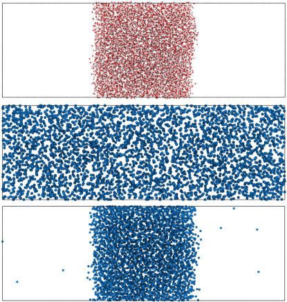
Figure 5: Simulation snapshots of droplets using the various models discussed. Top: all-atom TIP3P; middle: SS IBI; bottom: MS IBI. Atomistic and MS IBI models agree, producing a system with a stable interface, whereas SS IBI does not form a stable interface.

It is also important that the potential is not so strong that the system can solidify at physiological conditions. For example, the MARTINI water model is known to spontaneously crystallize at physiologically relevant temperatures.¹⁷ This phenomenon is enhanced by the presence of interfaces (e.g., a lipid bilayer surface), and requires the addition of unphysical “antifreeze” particles to avoid crystallization. While we note that modifications to the MARTINI water model exist (e.g., adding charge polarization),^{38, 39} only the original MARTINI model was tested, since it more closely resembles the model derived via MS IBI (i.e., both represent 4 water molecules as a single, spherically symmetric interaction site). To test the crystallization tendency, a nucleation site is generated with the following protocol. A crystalline state is generated by running a simulation with the MS IBI potential in the NVT ensemble. During this simulation, the temperature is decreased from 305 K to 1 K over 10 ns. A subsequent CG simulation is run at 1000 K, where the middle-most 1/8th of the beads are kept fixed, resulting in a configuration that contains a crystal seed surrounded by a fluid of CG water beads. The beads in the crystal seed are kept fixed in the nucleation site simulations, with interactions identical to the fluid interactions. While neither models shows a tendency to freeze at 305 K in the absence of a nucleation site over 100 ns of simulation, the MARTINI model rapidly crystallizes in the presence of a nucleation site, while the MS IBI potentials remains fluid (6). Note, for a direct comparison with the MS IBI model derived here, antifreeze particles were not used with the MARTINI model. To ensure that the MS IBI system is not an amorphous solid structure, the ratio of the diffusion coefficients with and without a nucleation site were calculated for each model. As shown in Table 2, the diffusion coefficient of the MS IBI potential model remains relatively unchanged when a nucleation site is added, whereas a significant drop is seen for the MARTINI model, resulting from crystallization. Additionally, Figure 7 plots the RDF of the MARTINI model for the bulk NVT state as compared to the 4:1 mapped target data. Clearly, the MARTINI potential does not accurately capture the structural correlations of bulk water, further demonstrating the significant improvement of the MS IBI model in reproducing key properties of water.

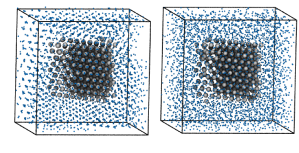
Figure 6: Configurations from simulations in the presence of a nucleation site with the MARTINI (left) and MS IBI (right) models. CG water beads colored silver were kept fixed during the simulations, but were treated as the same type as blue particles (i.e., the color is different to show the nucleation site).

Table 2: Ratio of diffusion coefficients from simulations with ($D_{nuc}$) and without ($D_{bulk}$) a nucleation site with different potentials. Diffusion coefficient $D$ calculated from the slope of a linear fit to the long-time MSD, using $MSD=6Dt$.

Model	$D_{nuc}/D_{bulk}$
MS IBI	0.88
MARTINI	0.02

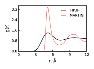
Figure 7: RDFs of the MARTINI model and the atomistic TIP3P model mapped to the CG level for the bulk NVT state.

4 Conclusions

In this work, the MS IBI method was used to derive the interactions for a 4:1 mapped CG water model. An improvement over previous models is made by simultaneously matching the fluid structure to target data from bulk and interfacial states. It was shown that a model that reproduces the structure and density of water does not necessarily reproduce the interfacial properties and that the addition of a droplet target state constrains the potential to also capture the interfacial properties. The resulting potential is able to accurately predict the density of water at 305 K at 1 atm, interfacial properties, and structural correlations. Additionally, the model shows no tendency to spontaneously crystallize at physiological conditions. This is important, since inaccuracies in a water model can propagate as more potentials are derived against it when simulating mixed systems.

This work highlights a key advantage of deriving potentials via the MS IBI approach. For simulations that cover multiple states, it is important to have a forcefield that is accurate across the states of interest. MS IBI allows this to be achieved by including target data from states that represent structures present in the states of interest. This is realized here by including a multi-ensemble state to accurately model the pressure-density relationship, and a droplet state to capture the interfacial properties. Another case where this would be beneficial is studying systems over multiple phases, e.g., phase transitions in liquid crystals. While clever approaches are taken to capture behavior across multiple states,⁴⁰ a more systematic approach would be useful. Based on the results presented here, we foresee this method being useful for deriving CG potentials for a wide range of applications.

References

- Wang and Voth 2005 Wang, Y.; Voth, G. A. Unique spatial heterogeneity in ionic liquids. Journal of the American Chemical Society 2005, 127, 12192–12193
- Bhargava et al. 2007 Bhargava, B. L.; Devane, R.; Klein, M. L.; Balasubramanian, S. Nanoscale organization in room temperature ionic liquids: a coarse grained molecular dynamics simulation study. Soft Matter 2007, 3, 1395–1400
- Karimi-Varzaneh et al. 2010 Karimi-Varzaneh, H. A.; Müller-Plathe, F.; Balasubramanian, S.; Carbone, P. Studying long-time dynamics of imidazolium-based ionic liquids with a systematically coarse-grained model. Physical Chemistry Chemical Physics 2010, 12, 4714–4724
- Padding and Briels 2002 Padding, J.; Briels, W. Time and length scales of polymer melts studied by coarse-grained molecular dynamics simulations. The Journal of Chemical Physics 2002, 117, 925–943
- Harmandaris et al. 2010 Harmandaris, V. A.; Floudas, G.; Kremer, K. Temperature and pressure dependence of polystyrene dynamics through molecular dynamics simulations and experiments. Macromolecules 2010, 44, 393–402
- Sun and Faller 2006 Sun, Q.; Faller, R. Crossover from unentangled to entangled dynamics in a systematically coarse-grained polystyrene melt. Macromolecules 2006, 39, 812–820
- Milano and Müller-Plathe 2005 Milano, G.; Müller-Plathe, F. Mapping atomistic simulations to mesoscopic models: A systematic coarse-graining procedure for vinyl polymer chains. The Journal of Physical Chemistry B 2005, 109, 18609–18619
- Shinoda et al. 2008 Shinoda, W.; DeVane, R.; Klein, M. L. Coarse-grained molecular modeling of non-ionic surfactant self-assembly. Soft Matter 2008, 4, 2454–2462
- Lee and Pastor 2011 Lee, H.; Pastor, R. W. Coarse-grained model for PEGylated lipids: effect of PEGylation on the size and shape of self-assembled structures. The Journal of Physical Chemistry B 2011, 115, 7830–7837
- Srinivas et al. 2004 Srinivas, G.; Discher, D. E.; Klein, M. L. Self-assembly and properties of diblock copolymers by coarse-grain molecular dynamics. Nature Materials 2004, 3, 638–644
- Nguyen and Hall 2004 Nguyen, H. D.; Hall, C. K. Molecular dynamics simulations of spontaneous fibril formation by random-coil peptides. Proceedings of the National Academy of Sciences of the United States of America 2004, 101, 16180–16185
- Iacovella et al. 2011 Iacovella, C. R.; Keys, A. S.; Glotzer, S. C. Self-assembly of soft-matter quasicrystals and their approximants. Proceedings of the National Academy of Sciences of the United States of America 2011, 108, 20935–20940
- Hadley and McCabe 2012 Hadley, K. R.; McCabe, C. Coarse-Grained Molecular Models of Water : A Review. Molecular Simulation 2012, 38, 671–681
- Basdevant et al. 2004 Basdevant, N.; Borgis, D.; Ha-Duong, T. A semi-implicit solvent model for the simulation of peptides and proteins. Journal of Computational Chemistry 2004, 25, 1015–1029
- Basdevant et al. 2006 Basdevant, N.; Ha-Duong, T.; Borgis, D. Particle-based implicit solvent model for biosimulations: Application to proteins and nucleic acids hydration. Journal of Chemical Theory and Computation 2006, 2, 1646–1656
- Masella et al. 2011 Masella, M.; Borgis, D.; Cuniasse, P. Combining a polarizable force-field and a coarse-grained polarizable solvent model. II. Accounting for hydrophobic effects. Journal of Computational Chemistry 2011, 32, 2664–2678
- Marrink et al. 2007 Marrink, S. J.; Risselada, H. J.; Yefimov, S.; Tieleman, D. P.; de Vries, A. H. The MARTINI force field: coarse grained model for biomolecular simulations. The Journal of Physical Chemistry B 2007, 111, 7812–7824
- Chiu et al. 2010 Chiu, S.-w.; Scott, H. L.; Jakobsson, E. A Coarse-Grained Model Based on Morse Potential for Water and n-Alkanes. Journal of Chemical Theory and Computation 2010, 6, 851–863
- Shinoda et al. 2007 Shinoda, W.; DeVane, R.; Klein, M. L. Multi-property fitting and parameterization of a coarse grained model for aqueous surfactants. Molecular Simulation 2007, 33, 27–36
- Hadley and McCabe 2010 Hadley, K. R.; McCabe, C. On the investigation of coarse-grained models for water: balancing computational efficiency and the retention of structural properties. The Journal of Physical Chemistry B 2010, 114, 4590–4599
- Van Hoof et al. 2011 Van Hoof, B.; Markvoort, A. J.; Van Santen, R. a.; Hilbers, P. a. J. The CUMULUS coarse graining method: Transferable potentials for water and solutes. Journal of Physical Chemistry B 2011, 115, 10001–10012
- Reith et al. 2003 Reith, D.; Pütz, M.; Müller-Plathe, F. Deriving effective mesoscale potentials from atomistic simulations. Journal of Computational Chemistry 2003, 24, 1624–1636
- Moore et al. 2014 Moore, T. C.; Iacovella, C. R.; McCabe, C. Derivation of coarse-grained potentials via multistate iterative Boltzmann inversion. The Journal of Chemical Physics 2014, 140, 224104
- Hadley and McCabe 2010 Hadley, K.; McCabe, C. A coarse-grained model for amorphous and crystalline fatty acids. The Journal of chemical physics 2010, 132, 134505
- Bayramoglu and Faller 2012 Bayramoglu, B.; Faller, R. Coarse-grained modeling of polystyrene in various environments by iterative boltzmann inversion. Macromolecules 2012, 45, 9205–9219
- Qian et al. 2008 Qian, H.-J.; Carbone, P.; Chen, X.; Karimi-Varzaneh, H. A.; Liew, C. C.; Müller-Plathe, F. Temperature-transferable coarse-grained potentials for ethylbenzene, polystyrene, and their mixtures. Macromolecules 2008, 41, 9919–9929
- Hartigan and Wong 1979 Hartigan, J. A.; Wong, M. A. Algorithm AS 136: A k-means clustering algorithm. Applied Statistics 1979, 28, 100–108
- Jorgensen et al. 1983 Jorgensen, W. L.; Chandrasekhar, J.; Madura, J. D.; Impey, R. W.; Klein, M. L. Comparison of simple potential functions for simulating liquid water. The Journal of Chemical Physics 1983, 79, 926–935
- Plimpton 1995 Plimpton, S. Fast parallel algorithms for short-range molecular dynamics. Journal of Computational Physics 1995, 117, 1–19
- 30 LAMMPS WWW Site - http://lammps.sandia.gov, \urlhttp://lammps.sandia.gov
- 31 A Git repository for this package is hosted at https://github.com/ctk3b/msibi., \urlhttp://github.com/ctk3b/msibi
- Anderson et al. 2008 Anderson, J. A.; Lorenz, C. D.; Travesset, A. General purpose molecular dynamics simulations fully implemented on graphics processing units. Journal of Computational Physics 2008, 227, 5342–5359
- Glaser et al. 2015 Glaser, J.; Nguyen, T. D.; Anderson, J. A.; Lui, P.; Spiga, F.; Millan, J. A.; Morse, D. C.; Glotzer, S. C. Strong scaling of general-purpose molecular dynamics simulations on GPUs. Computer Physics Communications 2015, 192, 97–107
- 34 HOOMD-Blue web page - http://codeblue.umich.edu/hoomd-blue, \urlhttp://codeblue.umich.edu/hoomd-blue
- McGibbon et al. 2014 McGibbon, R. T.; Beauchamp, K. A.; Schwantes, C. R.; Wang, L.-P.; Hernández, C. X.; Harrigan, M. P.; Lane, T. J.; Swails, J. M.; Pande, V. S. MDTraj: a modern, open library for the analysis of molecular dynamics trajectories. bioRxiv 2014,
- 36 A Git repository for this package is hosted at https://github.com/mdtraj/mdtraj., \urlhttp://github.com/ctk3b/msibi
- Wang et al. 2009 Wang, H.; Junghans, C.; Kremer, K. Comparative atomistic and coarse-grained study of water: What do we lose by coarse-graining? The European Physical Journal E 2009, 28, 221–229
- Yesylevskyy et al. 2010 Yesylevskyy, S. O.; Schäfer, L. V.; Sengupta, D.; Marrink, S. J. Polarizable water model for the coarse-grained MARTINI force field. PLoS Computional Biology 2010, 6, e1000810
- Zavadlav et al. 2015 Zavadlav, J.; Melo, M. N.; Marrink, S. J.; Praprotnik, M. Adaptive resolution simulation of polarizable supramolecular coarse-grained water models. The Journal of Chemical Physics 2015, 142, 244118
- Mukherjee et al. 2012 Mukherjee, B.; Delle Site, L.; Kremer, K.; Peter, C. Derivation of coarse grained models for multiscale simulation of liquid crystalline phase transitions. The Journal of Physical Chemistry B 2012, 116, 8474–8484