Towards physics responsible for large-scale Lyman-$\alpha$ forest bias parameters

Abstract

Using a series of carefully constructed numerical experiments based on hydrodynamic cosmological SPH simulations, we attempt to build an intuition for the relevant physics behind the large scale density ($b_{\delta}$) and velocity gradient ($b_{\eta}$) biases of the Lyman-$\alpha$ forest. Starting with the fluctuating Gunn-Peterson approximation applied to the smoothed total density field in real-space, and progressing through redshift-space with no thermal broadening, redshift-space with thermal broadening and hydrodynamicaly simulated baryon fields, we investigate how approximations found in the literature fare. We find that Seljak’s 2012 analytical formulae for these bias parameters work surprisingly well in the limit of no thermal broadening and linear redshift-space distortions. We also show that his $b_{\eta}$ formula is exact in the limit of no thermal broadening. Since introduction of thermal broadening significantly affects its value, we speculate that a combination of large-scale measurements of $b_{\eta}$ and the small scale flux PDF might be a sensitive probe of the thermal state of the IGM. We find that large-scale biases derived from the smoothed total matter field are within 10-20% to those based on hydrodynamical quantities, in line with other measurements in the literature.

1 Introduction

Measuring the growth of large scale structure has become a powerful probe of testing cosmological parameters. The Lyman-$\alpha$ forest has emerged as one of the primary tracers of this large scale structure at intermediate redshifts. Seen as absorption features in quasar spectra, the forest probes the distribution of neutral hydrogen between the observer and the quasar. The Lyman-$\alpha$ absorption of neutral hydrogen has a particularly large cross section, and as the emission continuum of a quasar becomes redshifted to this transition wavelength, it will be absorbed even with small fractions of neutral hydrogen present. This method is therefore sensitive to low gas densities, serving as a tracer of the large scale matter distribution between the redshifts of 1.7 (below which the gas becomes fully ionised while at the same time the UV light continuum becomes redshifted to wavelengths absorbed by the atmosphere) and redshifts 4-5 (above which the forest becomes opaque). At small scales, the Lyman-$\alpha$ forest has given us unique constraints on, for example, warm dark matter models [1, 2] and primordial black hole dark matter [3], whereas on intermediate scales it has probed limits on the sum of the neutrino masses [4, 5, 6], the running of the spectral index [6], or dark matter - baryon scattering [7]. Recently, at large scales, it has provided a detection of the baryon acoustic oscillations at intermediate redshifts [8, 9, 10]. With the completion of the BOSS survey [11], and the start of eBOSS [12], as well as the planned DESI survey [13], future Lyman-$\alpha$ forest measurements will be covering larger scales with greater precision. It is therefore crucial that we also improve our understanding of the biases involved between what is observed and the underlying matter distribution.

The relationship between the measured Lyman-$\alpha$ forest flux and the underlying matter is highly nonlinear, but the physics is thought to be well-understood. Underlying neutral hydrogen gas is related to this measured flux via the optical depth, $\tau=-\mathrm{ln}F$, which is proportional to the Lyman-$\alpha$ absorption cross section and the number of neutral hydrogen atoms along the line of sight (los). If photoionization equilibrium at these redshifts is assumed, the amount of neutral hydrogen is related in a temperature-dependent way to the total number of hydrogen atoms, which in turn traces the underlying matter density. Additionally, assuming adiabatic expansion, which produces a tight temperature-density relation, $\gamma-1=d\mathrm{ln}\rho/d\mathrm{ln}T$ [14], the optical depth can be modeled as $\tau=A(1+\delta)^{\alpha}$, where $\delta$ is the gas overdensity, $A$ is a constant which depends on the photoionization rate, the temperature of the gas, and redshift, while $\alpha=2-0.7(\gamma-1)$. The gas overdensity traces the total matter overdensity down to the Jeans scale, where gas pressure supports against gravitational collapse.

This Fluctuating Gunn Peterson Approximation (FGPA) [15], although it ignores shock heated gas and thermal broadening, has been surprisingly successful in explaining statistical properties of the Lyman-$\alpha$ forest observations. Because it is a local transformation, the flux fluctuations, defined as $\delta_{F}=F/\bar{F}-1$ (with $\bar{F}$ being the mean absorbed flux) will trace the dynamically dominant fields on large scales [16, 17]:

$$\delta_{F}=b_{\delta}\delta+b_{\eta}\eta+b_{\Gamma}\delta_{\Gamma}+\epsilon.$$ (1.1)

This equation is valid in Fourier-space in the limit $k\rightarrow 0$ or on a sufficiently smoothed real-space field (i.e where fluctuations are smoothed so that the Taylor expansion in $\delta$ is valid). The quantities $\delta$, $\delta_{\eta}$ and $\delta_{\Gamma}$ are relative fluctuations in the total density, mass-weighted velocity gradient $\eta=-H^{-1}dv_{||}/dr_{||}$ and photo-ionization fluctuations rate $\Gamma$. The bias parameters $b_{\delta}$, $b_{\eta}$ and $b_{\Gamma}$ encode properties of the small-scale physics that determines their values on large-scales. In this paper we will use these symbols to denote absorbed flux fluctuation ($\delta_{F}$) biases, but biases for other fields will denote tracer field, e.g. $b_{\tau,\delta}$ for the density bias of the $\delta_{\tau}$ field (all tracer fields will be normalized to the mean). Finally, $\epsilon$ describes the scatter between the tracer field $\delta_{F}$ and the prediction from source fields. It is expected to have a white power $P_{N}$ on large scales. We will not consider photoionization fluctuations in this paper, but see e.g.[18, 19] and references there-in.

Ignoring the $\Gamma$ field, it then follows that the three-dimensional power-spectrum of flux on large scales is given by

$$P_{\delta_{F}}(\bm{k})=b_{\delta}^{2}\left(1+\beta\mu^{2}\right)^{2}P_{\delta}(k)+P_{N}$$ (1.2)

where $\beta=fb_{\eta}/b_{\delta}$, with $f$ being the logarithmic growth rate, $\mu$ is the cosine of the angle between the los and the vector $\bm{k}$, and $P_{\delta}$ is the total matter power spectrum. This is equivalent to the famous Kaiser [20] redshift-space distortion (RSD) formula for galaxies, but note that in our case $\beta$ is not uniquely determined by $b_{\delta}$, as we will discuss later in the paper. The noise power $P_{N}$ is expected to be small and is often ignored.

Parameters $b_{\delta}$ and $b_{\eta}$ (or equivalently $\beta$) can be thought of as purely phenomenological parameters to be marginalised over as is done in e.g. BAO analyses. On the other hand they encode the same small scale physics that is used when predicting small scale 1D power spectra that has been used to constrain cosmology. Therefore, with a goal to eventually be able to perform a unified analysis of correlations in the Lyman-$\alpha$ forest, from smallest to the largest available scales, rather then artificially splitting the problem into a small-scale 1D power spectrum and a large-scale correlation function, the underlying physics that determines the values of these parameters has to be well-understood.

This paper attempts to bring some understanding to what determines the numerical value of these large-scale biases and how well these can be described using analytical predictions. The main focus in this study is not on using these predictions for precision cosmology, but primarily to first understand how accurate these predictions are or when do they fail in describing results of $N$-body simulations. This expands and complements previous work trying to understand the large scale fluctuations in the Lyman-$\alpha$ forest [21, 22, 16, 23, 24, 25, 17].

2 Theory

The basic starting point for derivation of biases is the notion of peak-background split (PBS), namely that a large over-dense region of the universe is equivalent to a slightly over-dense universe and that a large region of universe with non-zero $\eta$ is equivalent to an anisotropic universe with a velocity gradient. This picture is exact in the $k\rightarrow 0$ limit and gives the following simple prescription for the calculation of bias parameters[16, 26, 17]:

$$b_{\delta} = \frac{1}{\bar{F}}\frac{d\bar{F}}{d\delta}|_{\eta=0}$$ (2.1)

$$b_{\eta} = \frac{1}{\bar{F}}\frac{d\bar{F}}{d\eta}|_{\delta=0}$$ (2.2)

These formulae can be used both in theoretical modeling and in simulations.

This approach was used by [26] to make a first analytical attempt at understanding the large scale bias and redshift space distortion parameter. By using the second order perturbation theory gravitational coupling between short and long wavelength modes, analytical formulae can be obtained that link $b_{\delta}$ and $b_{\eta}$ to the observed flux probability distribution function (PDF).

Approximations used in that paper were

• The second order standard perturbation theory gives sufficiently accurate predictions bias of density field to $n$-th power

• The flux field is fully determined by the FGPA formula

  $$F=\exp\left[(-A(1+\delta)^{\alpha}\right]$$ (2.3)

• No thermal broadening of the lines

Somewhat surprisingly, we will later discover that the inaccuracy of these equations is mostly due to thermal broadening and the non-linearity of the velocity field.

2.1 Density bias

We will proceed to review the derivation of bias parameters. Our treatment is somewhat different from that of [26] in that it makes the peak-background argument more obvious, but we arrive at identical results. In the presence of a long wavelength density mode, $\delta_{l}$, in an Einstein-deSitter universe, the short wavelength density modes, $\delta_{s}$, in second order perturbation theory become

$$\delta_{s}^{\mathrm{pert}}=(1+\nu_{2}\delta_{l})\delta_{s},$$ (2.4)

where $\nu_{2}=34/21$, is the angular average of the second order perturbation theory kernel $F_{2}(\bm{k_{1}},\bm{k_{2}})$. This relation does not require that $\delta_{s}$ modes are linear, it simply provides an approximate mapping between a set of non-linear modes in a patch of universe as a function of large-scale over-density.

Therefore, the total density transforms as

$$\delta=\delta_{s}^{\mathrm{pert}}+\delta_{l}=(1+\nu_{2}\delta_{l})\delta_{s}+\delta_{l}.$$ (2.5)

The mean for a quantity $X$ in the presence of large-scale mode $\delta_{l}$ are thus given by

$$\bar{X}=\int_{-\infty}^{\infty}X(\delta=\delta(1+\nu_{2}\delta_{l})+\delta_{l})p(\delta)d\delta,$$ (2.6)

where $p(\delta)$ is the probability distribution function for $\delta$. Using Equation (2.1), this allows us to calculate bias for any quantity which is uniquely determined by $\delta$ and connect it to its PDF. Applying this to matter fields to the $n$-th power ($\delta^{n}$) (and normalizing by the mean of this tracer field), we find

$$b_{\delta^{n},\delta}=n\nu_{2}+n\langle\delta_{s}^{n-1}\rangle/\langle\delta_{s}^{n}\rangle.$$ (2.7)

The large scale bias for the Lyman-$\alpha$ forest  optical depth with respect to the underlying density is given by

$$b_{\tau,\delta}=\bar{\tau}^{-1}\frac{\partial\bar{\tau}}{\partial\delta_{l}}=\bar{\tau}^{-1}\nu_{2}\left\langle\delta\frac{d\bar{\tau}}{d\delta}\right\rangle+\bar{\tau}^{-1}\left\langle\frac{d\bar{\tau}}{d\delta}\right\rangle.$$ (2.8)

For the simple isothermal density-temperature relation, where $\alpha=2$, this gives

$$b_{\tau,\delta}=\frac{2(1+\nu_{2}\sigma^{2}_{J})}{1+\sigma^{2}_{J}},$$ (2.9)

where $\sigma_{J}$ is the rms density field smoothed on a Jeans scale.

The bias for optical depth is a theoretically interesting quantity, but it is not what we need. Ignoring redshift space distortions in the optical depth for now, the flux bias relating the flux to the underlying density field, can then be calculated as:

$$b_{\delta}=\frac{1}{\bar{F}}\frac{\partial\bar{F}[\tau({\delta)}]}{\partial\delta_{l}}=\frac{1}{\bar{F}}\left[\nu_{2}\left\langle\delta\frac{dF}{d\delta}\right\rangle+\left\langle\frac{dF}{d\delta}\right\rangle\right].$$ (2.10)

Using Equation 2.3, the above bias can be expressed in terms of the constants $A$ and $\alpha$:

$$b_{\delta}=\bar{F}^{-1}[\alpha\langle F\mathrm{ln}F\rangle+\alpha(\nu_{2}-1)\left\langle F\mathrm{ln}F[1-(-\mathrm{ln}F/A)^{-\alpha^{-1}}]\right\rangle].$$ (2.11)

Remarkably, therefore, this theoretical bias could be calculated from just the constants $A$ and $\alpha$, which could be derived from the temperature-density scatter plots from simulations, and the observed flux PDF in the data.

2.2 Velocity gradient bias

For the velocity gradient bias, consider the effect of $\eta$ on a large patch of the universe. The redshift-space coordinate $s=r+H^{-1}v_{\parallel}$ transforms as

$$s\rightarrow s-r\eta.$$ (2.12)

Action of the $\eta$ field is thus equivalent to stretching the redshift-space in the radial direction. Since stretching cannot change the total number of hydrogen atoms, the mean value of $\tau$ must change by $(1-\eta)^{-1}$ giving $b_{\tau,\eta}=1$. The same argument holds for all other fields that are conserved on transformation from real to redshift space (e.g. number of galaxies). In the limit of no thermal broadening, the $\tau$ simply responds as pure rescaling

$$\tau(r)\rightarrow\frac{\tau\left(r(1-\eta)^{-1}\right)}{1-\eta}=\tau\left(r(1-\eta)^{-1}\right)(1+\eta)+O(\eta^{2})$$ (2.13)

Using Equation 2.2,

$$\bar{F}=\int_{0}^{1}p(F)FdF$$ (2.14)

and $\tau=-\ln F$, one can derive

$$b_{\eta}=\left\langle F\mathrm{ln}F\right\rangle.$$ (2.15)

This equation was derived by Seljak by starting with the relation $\tau(\bm{s})=\tau(\bm{r})(1+f\mu^{2}\delta)$ and then Taylor expanding the expression for $F$. The above shows that it is in fact much more general and gives the correct answer on large scales even if the distortions are not Kaiser-like in $\tau$ on intermediate scales, as long as velocity dispersion is negligible. However, as we will see later, the presence of thermal broadening is significant and breaks this formula, since the broadening kernel does not stretch with the $(1-\eta)$ factor.

In this paper we use SPH simulations to test these analytical formulae. We start with the smoothed total matter field part of these simulations and apply the FPGA equation exactly in real space to see how well they fare in this idealised toy-case. We then proceed to progressively more realistic cases, ending with the analysis of the full hydrodynamic part of the simulation.

3 Description of Numerical Methods and Simulations Used

The simulations used for this comparison study are Gadget-3 [27] hydrodynamic simulations with a box size of $L=40$ $\mathrm{Mpc/h}$ with $N=2\times 1024^{3}$ for the number of gas and dark matter particles. They are evolved with a Haardt and Madau UV background [28] and the simple QUICKLYA option for star formation with no feedback, where any SPH particle that reaches a maximum density is converted into a star particle. The standard critical over-density, as used in these simulations, is 1000 times the mean. The SPH smoothing length is such that the particle’s density is estimated by smoothing over 32 neighboring particles. The fiducial simulation uses the WMAP7 cosmology.

In the following, we start with simply analyzing the density field from these hydrodynamic simulations, using the total matter overdensity output $\delta$ from the simulation at each point to transform to a flux field via the FGPA in Equation 2.3. We progressively add the redshift space distortions (RSD), and thermal broadening by hand to this flux field as described below in Section 4. Before applying the FGPA to the density field, we smooth it using a Gaussian filter $\delta(k)\to\delta(k)\mathrm{exp}(-k^{2}R^{2}/2)$ to account for Jeans smoothing present in baryon fields. We always measure our quantities at different levels of smoothing, including unrealistically large smoothing factors, since analytical expressions are expected to perform better at more aggressive levels of smoothing. Unless stated otherwise, we assume $A=0.3((1+z)/(1+2.4))^{4.5}$ and $\alpha=1.6$ as in [26]. Finally, it is only in Section 6, that we analyze the flux field from the hydrodynamic part of these same simulations, in order to compare it to the one generated from this FGPA prescription.

We calculate true bias parameters using two methods, which we describe in the following two sub-sections.

3.1 Peak-background split applied to simulations

This amounts to numerically evaluating expressions in Equations 2.1 and 2.2 and has been used to measure the bias parameter by McDonald well over a decade ago [16].

$\delta(z=2.5)$	-0.015	0.0	0.015
$\Omega_{m}(z=0)$	0.260	0.275	0.290
$\Omega_{k}(z=0)$	0.024	0.0	-0.024
$\Omega_{\Lambda}(z=0)$	0.715	0.725	0.735
$h0$	0.707	0.702	0.697
$\sigma_{8}$	0.795	0.816	0.836

Table 1: Parameters of peak-background split simulations.

For density simulations, this entails running two additional simulations, acting as over- and underdense counterparts to the fiducial simulation. In order to achieve this, the starting cosmological parameters for these simulations have to be changed. The main requirement is for the density in the perturbed universe to satisfy $\rho^{\prime}(t)=\rho(t)(1+\delta_{l}(t))$, where $\delta_{l}$ represents the matter overdensity with respect to the background universe (which can be thought of as the long wavelength mode overdensity in this region of the universe). From this relation, the cosmologies for the perturbed simulations can be derived. Requiring a $\delta_{l}$ value of $+/-0.015$ at $z=2.5$ (the central redshift of interest for the Lyman-$\alpha$ forest ), the perturbed cosmological parameters in Appendix A can be evaluated at $z=0$ to give the values in Table 1. All three simulations listed in Table 1 are evolved from $z_{i}=159$ with outputs at $z=$ 3, 2.8, 2.75, 2.6, 2.5, 2.4, 2.25, 2.2, and 2. Here we focus our analysis on redshifts 3, 2.5, and 2. Since the evolution of redshift with time is different in the perturbed universe we rescale the density field of the perturbed simulation from the nearest redshift output $z$ to match the required $z^{\prime}$ as seen in Equation A.4 using the growth factor. (The matching $z^{\prime}$ for example to $z=2.5$ is $z^{\prime}=2.47$ for $\delta_{l}=+0.015$). We check that this scaling matches the results achieved by interpolation methods to better than $0.01\%$.

After the perturbed simulation density fields are rescaled to the correct redshift, the over-densities are further rescaled to be expressed with respect to the the mean of the unperturbed simulation by $\delta^{\mathrm{pert}}\to\delta^{\mathrm{pert}}(1+\delta_{l})+\delta_{l}$. This $\delta^{\mathrm{pert}}$ is then used to calculate the mean flux in the FGPA approximation when computing the numerical derivative in Equations 2.1 and 2.2 for the peak background split method analysis.

For the velocity gradient bias, the calculation is less painful. The prescription in Equation 2.12 postulates that we need to imagine our simulation box is now of the size $L^{2}\times L(1-\eta_{l})$, where we set $\eta_{l}=\pm 0.01$ to be the long-scale $\eta$ we differentiate with respect to. This means that before calculating the mean quantities, we need to i) divide all $\tau$’s by $(1-\eta_{l})$ and ii) divide the thermal broadening parameter by $(1-\eta_{l})$. These are precisely the prescriptions that McDonald gives in his 2003 paper [16].

3.2 Direct mode-by-mode measurement

As a cross-check, we also calculate the bias parameters using the standard way by comparing the cross matter-trace power spectrum with the matter power spectrum. We formalize this by writing the likelihood assuming scatter $\epsilon$ to be normally distributed with variance $P_{N}$, i.e.

$$\log L={\rm const.}-\frac{N}{2}\log P_{N}-\sum_{{\rm modes\ i}}\left(\frac{(\delta_{F,i}-\delta_{F}(\delta,\eta,b_{\delta},b_{\eta}))^{2}}{2P_{N}}\right),$$ (3.1)

where $\delta_{F,i}$ are the actual measured flux modes and $\delta_{F}(\delta,\eta,b_{\delta},b_{\eta})=b_{\delta}\delta+b_{\eta}\eta$ is the corresponding prediction from actual total fluctuation modes $\delta_{i}$ and bias parameters. We maximize this likelihood over free parameters $b_{\delta}$, $\beta$, $P_{N}$ and their $k^{2}$ and $k_{\parallel}$ corrections (6 parameters in total) and use the second derivative matrix to derive the marginalised error assuming Gaussianity.

By analytically maximizing the likelihood, one can show that this measurement is essentially the same as measuring the bias from the ratio of the cross-power to the dark matter auto-power spectrum. Measuring bias from the cross-power spectrum rather than the flux auto-power spectrum avoids biases due to the presence of the noise term $P_{N}$, but this is likely a very small effect. The main advantage of going through likelihood is that this method correctly propagates the scatter between the modes into an uncertainty in the bias determination.

We have tested this method extensively on toy problems. Nevertheless, to our great consternation, we note that while results are in general in good agreement with those from the peak-background split, there are cases where they disagree significantly. We believe that these are due to two kinds of effects. First, our box size of $40$ Mpc/h is limited and we do not correctly account for the effect of large-scale modes. This plagues the PB split method as well, but there at least the effect of $k=0$ mode is propagated correctly. In fact the fundamental mode, $k=2\pi/(40\ \mathrm{Mpc/h})$, is on the verge of being significantly non-linear at $z=2.5$. Second, although we correctly account for the $k^{2}$ dependence of bias parameters, we do not fit for other bias parameters that surely exist at this level, most importantly $b_{2}$ and $b_{s^{2}}$ [29] along with similar parameters for the $\eta$ field.

In [17], the authors take a somewhat different approach towards fitting bias parameters and fit the power spectrum measurement with an attempted guess at the shape of non-linear corrections to the $k\rightarrow 0$ limit. Despite having a larger box they similarly find that solutions are sensitive to details of the fitting formulae.

4 Results

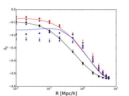
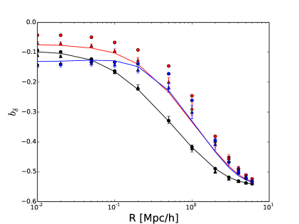
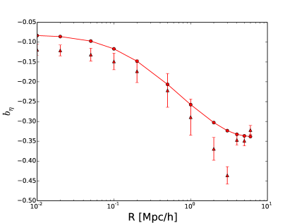
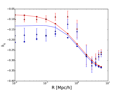
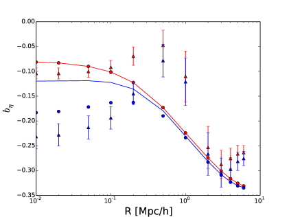
We now show our results through a series of plots that use the same symbol coding. Results from analytical predictions are plotted as lines, peak-background split results as dots and mode measurements as triangles with error-bars. These are usually plotted as a function of smoothing scale, unless noted otherwise.

4.1 Moments of the density field

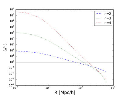
In Figure 1, we plot the theoretical bias for moments of the density field in our simulations together with predictions from Equation 2.7 for $n=2,3,$ and $4$. We see that even though $\delta^{4}$ becomes non-linear at $R>2$ Mpc/$h$, the bias predictions work surprisingly well down to $R\sim 0.3$ Mpc/h. In fact, as long as the variance of the field is not-significantly larger than unity, the predictions for $\delta^{n}$ bias are accurate, despite $\left<\delta^{n}\right>$ being large, presumably due to isolated high-density regions.

Figure 1: Upper left panel shows the mean value of moments of the matter field $\delta^{n}$ at redshift 2.5 as a function of smoothing scale. Other panels show their bias factors: from peak-background split (filled dots) and the analytical prediction (black line).

4.2 Taylor expansion approximation to the $\tau$ field

We start by a simple test, that is demonstrating the hopelessness of using a Taylor expansion in modeling the flux fluctuations. Namely, we can expand flux as

$$F=\exp\left(-\bar{\tau}\left(1+\delta_{\tau}\right)\right)=\exp\left(-\bar{\tau}\right)\left[1-\bar{\tau}\delta_{\tau}+\frac{1}{2}(\bar{\tau}\delta_{\tau})^{2}-\ldots\right]$$ (4.1)

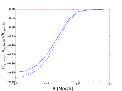
and then directly test the applicability of this expansion in simulations, by using a truncated Taylor expansion in place of an exponential when creating the flux field in simulations, but then proceeding to calculate biases as usual. Discrepancies between the truncated exponential expansion and the true field will show what is the best any analytically method based on Taylor-series expansion could do.

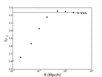
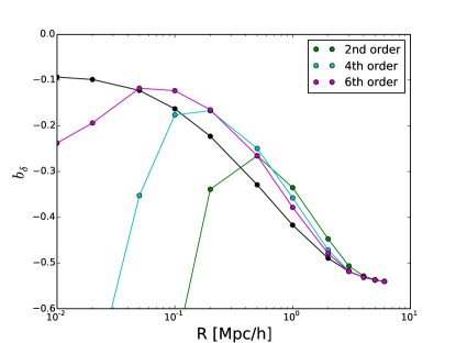
Results for the simple real-space FGPA bias are shown in Figure 2. We see that the expansion works fine at large smoothings, but fails to describe reality at small values of smoothing kernel size. This demonstrates that any approximations that attempt to describe the Lyman-$\alpha$ forest bias in terms of bispestrum, trispectrum, etc of the $\tau$ field are bound to fail. What really drives the change of the bias is the change in the flux PDF in the presence of the large-scale mode.

Figure 2: Density bias of the flux fluctuations after calculating the flux field as a Taylor expansion in optical depth around its mean (see text). The black line represents the full flux calculation (no Taylor expansion). The green line represents the Taylor expansion to 2nd order, the cyan represents 4th order, and magenta represents a 6th order expansion. All flux calculations are done for real-space FGPA with $A=0.34$ and $\alpha=1.6$ for $z=2.5$ using the peak-background split method described in the text.

4.3 Real-space FGPA

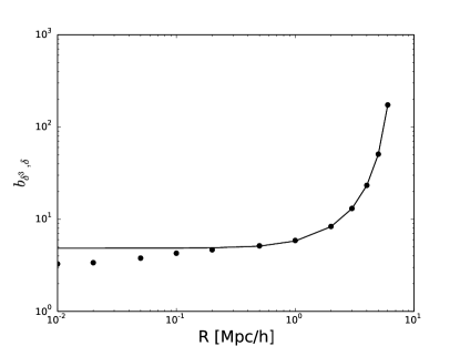
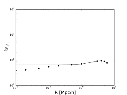
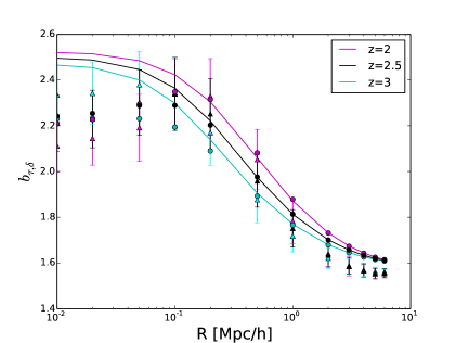
In Figure 3 we plot the corresponding predictions for $b_{\tau,\delta}$ and $b_{\delta}$ for real-space $\tau$. Analytical predictions agree remarkably well with measurements for this deterministic relation and are in fact much better than one would naively expect given Figure 1. We find that the agreement for flux is better than the agreement for the optical depth field. This is likely because the $\exp(-\tau)$ transformation suppresses the high-density regions where linear theory is supposed to break down.

Figure 3: Measured and predicted values of $b_{\tau,\delta}$ (left panel) and $b_{\delta}$ (right panel) in real space as a function of smoothing scale for $z=2$ (magenta, top), $z=2.5$ (black, middle) and $z=3$ (cyan, bottom). Solid lines are analytical formula predictions, solid points are PBS results and triangles mode fitting. Dashed lines show analytic predictions with $\nu_{2}=0$.

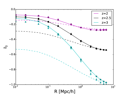The agreement between the theory and the measurement hinges on the transformation of the flux PDF on the modes as given by the second order linear calculation in Equation (2.5), which one would naively expect to be swamped by higher-order non-linear effects on small scales. This good agreement is not a coincidence. If we set $\nu_{2}=0$ (dashed line in Figure 3) we get completely wrong results, so the magic number $\nu_{2}=34/21$ stemming from second order standard perturbation theory is indeed crucial to the good fit we obtain in this case. As demonstrated in section 4.2, this success does not stem from the second order perturbation theory correctly capturing the bispectrum of $\tau$ fluctuations, but rather, it is because Equation (2.5) correctly captures how the flux PDF is transformed in the presence of the large-scale mode.

We also see that the analytical prediction works increasingly well with decreasing redshift, in correspondence with the decreasing value of $A$. With no smoothing ($R=0$), the analytical prediction is within $4\%$ of the peak-background split results for $z=2$, where $A=0.17$, within $6\%$ for $z=2.5$, where $A=0.34$, and within $18\%$ for $z=3$, where $A=0.62$. The analytical prediction therefore works best for low values of the optical depth, which decreases with decreasing redshift, despite the increase in the matter power spectrum. On the other hand, if $A$ is held artificially constant between redshifts at $A=0.34$, the corresponding values are $16\%$ for $z=2$ and $7\%$ for $z=3$, as expected, for linear theory to hold better at higher redshift. If the density field is smoothed with a smoothing factor of $R=0.2$ Mpc/h, thus decreasing the overall value of the optical depth, the analytical prediction is still within $4\%$ of the peak-background split results for $z=2$, where $A=0.17$, but now $0.6\%$ for $z=2.5$, where $A=0.34$, and within $0.8\%$ for $z=3$, where $A=0.62$.

The slightly worse agreement between the numerical and analytical methods at higher redshift is therefore driven by the increasing value of the normalization, $A$. The IGM is less ionized at these redshifts, resulting in a higher optical depth. The higher $A$ therefore may pick out the few extreme regions of the simulation, skewing the bias measurement towards these regions. Since the sample size of these regions inside the volume being probed by our simulations is small, the error on this measurement will be higher at larger redshift, limited by this sample variance.

4.4 Redshift-space FGPA

We introduce the redshift-space distortions in three different ways of increasing realism to test how well do theory predictions fare.

4.4.1 Linear Kaiser RSD

First, we impose the redshift-space distortions by simply adding them to the real-space $\tau$ FGPA field as expected in the linear theory:

$$\tau_{s}=\tau_{r}(1+f\mu^{2}\delta_{l})$$ (4.2)

This is justified by the fact that the $\tau$ field is conserved on real-redshift-space transformation and hence $b_{\tau,\eta}=1$. We refer to fields created in such a way as “linear Kaiser RSD” (lKRSD).

4.4.2 Linear velocity RSD

Next we produce an actual redshift-space $\tau$ by shifting the $\tau$ field around using appropriate velocities, following

$$\tau_{s}(s)=\int\tau(r)\delta_{D}(s-r-H^{-1}v)dr,$$ (4.3)

but actually using linear velocities $v_{k}=ifaH(a)\delta(k)\mu_{k}/k$ for this. We refer to this method of generating RSD as “linear velocity RSD” (lvRSD).

4.4.3 Non-linear velocity RSD

Finally, we use equation 4.3, but use actual non-linear baryon velocities. We refer to this method of generating RSD as “non-linear velocity RSD” (nlvRSD).

4.4.4 Thermal Broadening

In addition to the velocity offset in a simple RSD picture, the absorbing neutral hydrogen gas also has some thermal motion with respect to the background due having a gas temperature $T$. This additionally introduces a Gaussian line broadening profile:

$$\sigma_{\alpha}=\sigma_{0}\frac{c}{b\sqrt{\pi}}e^{-(\Delta v)^{2}/b^{2}},$$ (4.4)

where $\sigma_{\alpha}$ is the new cross section written in terms of the original Lyman-$\alpha$ absorption cross section at rest, $\sigma_{0}$, broadened by a Maxwellian velocity distribution of the gas with a Doppler parameter $b=\sqrt{2kT/m}$, where $m$ is the mass of the atom, and $\Delta v$ is the velocity difference with respect to the center of the absorption line.

In effect, RSD and thermal broadening together move the optical depth by a corresponding peculiar velocity and spread out the value at that point with a Gaussian profile to neighboring pixels with a width based on the temperature of the gas at the original point. We therefore expect thermal broadening to be degenerate with the $b_{\eta}$ value of the pure RSD, as these are both line-of-sight effects.

We use the tight temperature-density relation to introduce this thermal broadening, with $b^{2}=(12.8\mathrm{km}\mathrm{s}^{-1})^{2}\left(\frac{T_{0}}{10^{4}K}\right)(\delta+1)^{\gamma-1}$, and $\gamma-1=(2-\alpha)/0.7$ and $T_{0}=10^{4}K$.

4.4.5 Results

For the peak background split model calculations, we rescale and smooth the peculiar velocities just as the RSD density in the previous section (with an additional factor of $f$). We use this rescaled velocity field for the peak-background split calculation for the simple redshift space fields.

Figure 4: Flux bias parameter for $z=2.5$ and $A=0.34$ and $\alpha=1.6$, while varying the smoothing parameter $R$. Black represents real-space, red redshift space, and blue introducing redshift space and thermal smoothing, as described in the text. Lines, points and errorbars correspond to theory, PBS method and likelihood methods of bias determination. The top left panel corresponds to lKRSD, top right to lvRSD and bottom left to nlvRSD (see text for description of acronyms). The bottom right panel shows the difference between the analytical predictions and the PBS method. The dotted lines represent lKRSD, dashed lvRSD and solid nlvRSD.

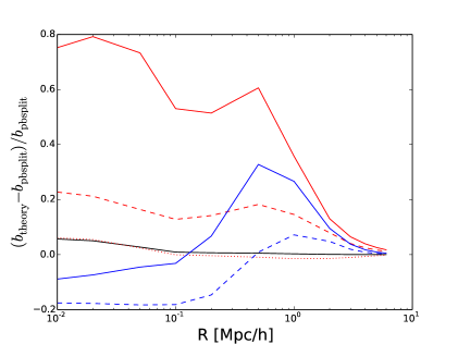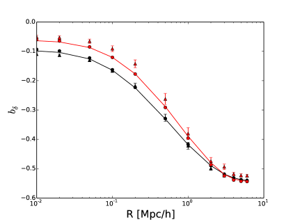
Our results for the flux density bias are displayed in Figure 4 in red. We see that as we progress towards more realistic redshift-space distortions, the theory predictions for the density bias remain in rough qualitative agreement with the measurements, but that the formula is accurate only to within an order of magnitude. Looking first at the PBS results, we note that while purely Kaiser distortions (lkRSD) seem to keep the predictivity of our formulae, even taking into account the non-linearities induced by actually moving the $\tau$ field around (instead of imposing $\mu^{2}$ distortions) already introduces errors at the level of 20%, which then increase even further when we go to correctly non-linear velocities. Adding thermal broadening correctly captures the decrease in bias at small smoothing, but underpredicts the overall effect. When thermal broadening is applied on nlvRSD, the formula is accurate to around 10% for $R=(10^{-2}-10^{-1})$Mpc/$h$, but this seems to be mostly due to fortuitous cancellation of errors (since it works worse in the case of lvRSD). We also note a surprising discrepancy between the likelihood method for measuring bias and the PBS in the case of nlvRSD and no thermal broadening. This can be directly tracked to the fact that there are missing velocity non-linearities in the 40 Mpc/h box that cause the offset in PBS measurements with respect to the theory predictions – if we replace the velocity field in the offset simulations with that of the original simulation, the difference between likelihood and PBS biases disappear.

Figure 5 shows the same for the velocity gradient bias. In this case, in case of no thermal broadening, the theory predictions are exact and show perfect agreement with the PBS method. Note however that the introduction of thermal broadening has a devastating effect on the accuracy of this prediction, making it underestimate the bias by up to 30%. However, we note that this difference could actually turn out to be a sensitive probe of the thermal broadening and thus the temperature of the IGM, but we defer this study for future work. Again we note curious discrepancies between the power spectrum bias predictions and the PBS, which are occasionally larger than what one would expect based on errors alone. Our tests indicate that this is unlikely due to underestimation of errors, but can be due to missing $\eta$ bias parameters and simply small box effects.

Figure 5: Same as Figure 4 but for $b_{\eta}$.

5 Dependence of $A$ and $\alpha$

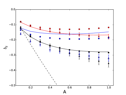
Figure 6 shows the dependence on the values of $A$ and $\alpha$ for a smoothing scale of $R=0.2$ Mpc/h for $z=2.5$. The agreement of the second-order analytical prediction of [26] with the peak-background split method in real-space is to within $10\%$ at this central redshift for a wide range of values for $A$ and $\alpha$. Again, a first-order perturbation theory with $\nu_{2}=0$ fails miserably.

Figure 6: Flux bias parameter for $z=2.5$ and $R=0.2$ Mpc/h, while varying the parameter $A$ at constant $\alpha=1.6$ (left panel) and varying $\alpha$ at constant $A=0.34$ (right panel) for lvRSD. Black represents real-space, red redshift space, and blue introducing redshift space and thermal smoothing. As before, solid lines are analytical formula predictions, solid points are PBS results and triangles mode fitting. Dashed lines show analytic predictions with $\nu_{2}=0$.

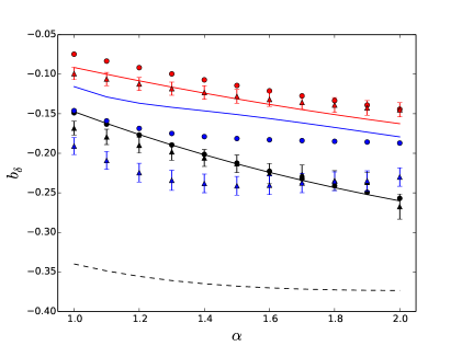However, after the redshift-space distortions are introduced, both methods seem to fail at about the same level, regardless of values of $A$ and $\alpha$ and only weakly capture the trends.

Again, we note an interesting discrepancy between PBS bias determination and the power spectrum based one, increasing towards large values of $A$. These correspond to more aggressively picking particular regions of the space where finite volume effects play a more important role.

6 Hydrodynamical fields

We now turn to the full hydrodynamic part of the simulation, taking the flux field generated directly from the simulation. We rescale the flux field to match the mean values of [30]. The analytical and likelihood bias methods are calculated directly from these fields, where the values of $A$ and $\alpha$ are taken from a smallest chi-squared fit of the real-space $\tau$ field with respect to the underlying density field.

However, for the peak-background split method, the situation is a bit more complex. We note that while the density field in the perturbed simulations evolve as expected with respect to the fiducial simulation, the ionizing background is evolved with the redshift of that simulation, not corresponding to the time of the fiducial simulation. We therefore have to rescale the fitted value of $A$ to fit that of the fiducial simulation at the same corresponding global time. This is further complicated by the fact that we do not have outputs of these perturbed simulations that would correspond to the exact same global time as those of the fiducial simulation (we do not have outputs at the values of $z^{\prime}$ as stated in Section 3.1). In order to circumvent this, we first interpolate (with a polynomial fit) the rescaling of $A$ in the fiducial simulation with respect to redshift, we then calculate the redshift of the fiducial simulation that would represent the same global time as the output of the perturbed simulation (for example, $z^{\prime}=2.5$ corresponds to a $z=2.53$ in the fiducial), and rescale the optical depth at that output according to the rescaling function of $A$ (in the example, this would correspond to rescale the perturbed simulation to match A(z=2.53)). After rescaling the optical depths to the appropriate values of $A$ at the output redshifts, we calculate the mean values of flux, and then again use an interpolating function for this mean flux as a function of redshift, to calculate the mean flux values at the appropriate values of $z^{\prime}$ according to Equation A4. This method introduces an error due to the interpolating functions, but could be rectified in the future by generating outputs of the perturbed simulations at the appropriate values of $z^{\prime}$.

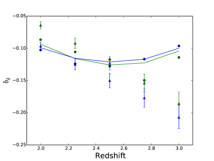
We compare this to the result of the FGPA + RSD (nlvRSD)+ thermal broadening method of the previous sections, with a smoothing value of $R=0.04$ Mpc/h, which corresponds to the value where the analytical predictions of the density bias in real-space flux fields were the closest to those of the real-space hydrodynamic flux predictions. The comparison is plotted in Figure 7.

Figure 7: Flux density bias (left) and velocity gradient bias (right) parameters for the hydrodynamic part of the simulation plotted in green with redshift, where the flux is scaled to match the means as measured by [30]. As a comparison, the result of the FGPA + RSD + thermal smoothing method of the previous sections is plotted in blue for the corresponding $A$ and $\alpha$ as fitted in the simulation, and appropriately scaled to the mean with a smoothing of $R=0.04$ Mpc/h. The corresponding symbols have the usual meaning, where triangles are the likelihood method calculation, circles the peak-background split result, while the solid lines are the analytical predictions.

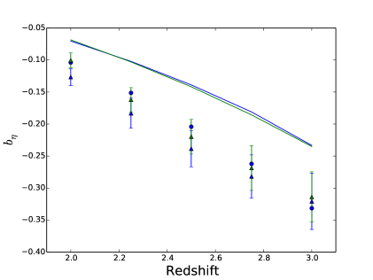It is hard to read too much into this figure, since the uncertainty in the flux determinations is significant. We chose a value of smoothing so that predictions based on the flux PDF are in closest agreement and these seem to be good to $10\%$. The numerical value of the smoothing is in the right ball-park but it is not the same as the filtering scale of [14]. We find decent agreement between FGPA approximated fields and hydrodynamical fields, especially at higher redshift.

We find a curious upturn in $b_{\delta}$ with redshift, both in the PBS determination of bias and the analytical predictions. This is likely the result of errors in our bias determination and a failure of analytical predictions at high values of $A$, since linear theory predicts a power-law change of bias with redshift [26]. Observations of the bias trend are consistent with our results for $2<z<2.5$ [31].

The above values calculated with the FGPA method also do not include scatter around the $\tau-\delta$ relation. We investigate the effect of scatter by incorporating a scatter term into the relation, where $\tau=\tau_{\mathrm{FGPA}}(1+\epsilon)$, following [26], where $\epsilon$ is taken from a normal distribution with a standard deviation of $\sigma_{\epsilon}=0.15$ as measured from the hydrodynamic part of our simulations. This amount of scatter results in the FGPA analytical predictions decreasing in absolute value by less than $1\%$ for both $b_{\delta}$, and $b_{\eta}$ at the central redshift of $z=2.5$, and is negligible for the numerical bias results. The addition of scatter therefore is not an important effect in the comparison above.

For the velocity bias results, we are not able to generate the peak-background split method result, but we present the likelihood method and the analytical prediction, again comparing to the FGPA + nlvRSD + thermal broadening methods in Figure 7. The hydrodynamic and FPGA fields are in good agreement with each other, but while the analytical formula for both nicely predicts the relative change in $b_{\eta}$ as a function of redshift, it fails to predict its absolute value. For both fields the absolute value of $b_{\eta}$ is within $27\%$ of the mode-by-mode fit for $z=2.0$, growing to a slightly worse agreement at $z=3.0$, where the absolute value of the analytical prediction is within $37\%$ of the simulation mode-by-mode fit.

7 Discussion & Conclusions

We have applied the FGPA framework in order to test the analytical form for the flux density bias and the velocity gradient bias against the numerical methods of the peak background split numerical derivative and the mode-by-mode likelihood fit. We have found that the short scale density perturbations evolve as predicted by the second-order perturbation theory assumed by [26] in the expected regime ($\delta<1$). This is also reflected in the optical depth fluctuations bias, which agrees with the numerical methods in the same regime.

When we turn to the flux bias, however, the analytical method seems to work surprisingly better than for the optical depth bias, agreeing even in the smallest smoothing scales with the numerical methods. This may be a reflection of the fact that, unlike the optical depth, flux becomes more sensitive to the accurate description of less dense regions, where in the real space FGPA framework, $F=\mathrm{exp}(-A(1+\delta)^{\alpha})$, the higher densities are suppressed. Indeed, the analytical prediction of the flux bias in Equation 2.11, as discussed in [26], is very sensitive to void regions. These less dense, void regions, are exactly where linear and second order perturbation theory correctly describe the mapping between densities in a typical region and an equivalent matter distribution riding a large-scale over or under-density. Thus the analytical form of the bias based on these assumptions will hold especially well for the flux field. An argument supporting this idea is that Taylor-expanding the optical depth field to a finite order does not reproduce the bias to the same accuracy and hence it is not the predictions of the 2- or 3-point functions that make the 2nd order perturbation theory work but instead the sucess in describing the matter density PDF change in the relevant regime.

When we introduce redshift space distortions, the predictions for the density bias parameter becomes considerably less accurate. By attempting increasingly realistic ways of introducing the redshift-space distortions we note that this is associated with non-linear mapping between real and redshift-space even for linear velocities. Adding thermal broadening further degrades any agreement.

For the velocity gradient bias we show that the expression given in [26] is exact in the limit of no thermal broadening. Our numerical results support this conclusion, effectively by construction. However, when thermal broadening is taken into account the predictions can be off considerably amounts. This indicates that an appropriate combination of measurements of the small scale flux PDF and the large scale bias parameters might provide a path towards robust measurements of the thermal state of the IGM.

Finally, we measure bias parameters from simulations using two different methods: a peak-background split method and direct mode-by-mode cross power spectrum method. While we find that they in general agree very well, we have found evidence that our 40 Mpc/h boxes still suffer from finite box effects and that “one loop” bias parameters and noise contributions might be important. It is crucial that a physics-based parameterization of the Lyman-$\alpha$ forest bias parameters is developed, especially to allow for a robust measurement from finite-sized boxes. We find that bigger $A$ values might put more emphasis on the more extreme/void regions of the density box, skewing the bias measurements towards these regions which are not well represented by the size of the box. At the same time, the fundamental $k$ mode for the mode-by-mode fit is on the verge of being non-linear. Therefore further studies will need to include bigger box size simulations to fully understand this discrepancy.

We also note that precise measurements using multiple boxes in the PBS formalism is difficult to do precisely: even if one has outputs at the precise redshifts (something we do not have), there are errors associated with external non-gravitational inputs such as reionization which is parameterized by redshift and hence occurs at slightly wrong times in offset boxes. For the future, it is therefore probably easier to inject a single mode with large amplitude into a single box and measure bias values off that particular mode.

We conclude that while analytical methods can provide good insight into the inner workings of the biasing of the Lyman-$\alpha$forest, they ultimately fail to provide sufficient accuracy for precision cosmology. This is not due to their description of non-linear density field, since the match is excellent for real-space flux, but rather the messiness of small-scale velocity effects.

Appendix A Parameters of peak-background perturbed simulations

Here we derive the parameters needed to evolve an over- or under-dense simulation, representing over- or under-dense regions of the fiducial cosmology. The main requirement is such that $\rho^{\prime}(t)=\rho(t)(1+\delta_{l}(t))$, where $\delta_{l}$ represents the matter overdensity with respect to the background universe (which can be thought of as the long wavelength mode overdensity in this region of the universe). This $\delta_{l}$ evolves linearly with the growth factor such that $\delta_{l}(t)=D(t)\delta_{0}$ and $d\delta_{l}(t)/dt=H(t)f(t)\delta_{l}(t)$, with $D(t)$ is the linear growth factor, $\delta_{0}$ is the value of $\delta_{l}$ at $z=0$, and $f(t)$ is the derivative of the logarithmic growth factor.

Since $\rho(a)\propto a^{-3}$ and $\mathrm{dln}\rho/\mathrm{d}t=\mathrm{dln}\rho/\mathrm{d}a\dot{a}=-3H(t)$, one can derive the hubble parameter for the perturbed simulation to first order in the long overdense mode:

$$\frac{\mathrm{dln}\rho^{\prime}(t)}{\mathrm{d}t} =\frac{\mathrm{d}}{\mathrm{d}t}\left(\mathrm{ln}\rho(t)+\mathrm{ln}\left(1+\delta_{l}(t)\right)\right)$$

$$-3H^{\prime}(t) \approx-3H(t)+H(t)f(t)\delta_{l}(t)$$

$$H^{\prime}(t) \approx H(t)\left(1-\frac{1}{3}f(t)\delta_{l}(t)\right).$$ (A.1)

Using this result we can derive the value of $\Omega_{m}$ for the perturbed simulation, again to first order in the perturbed wavelength:

$$\rho^{\prime}(t) =H^{\prime}(t)\Omega_{m}^{\prime}(t)=H^{2}(t)\Omega_{m}\left(1+\delta_{l}(t)\right)$$

$$\Omega_{m}^{\prime} \approx\Omega_{m}\left[1+\left(1+\frac{2}{3}f(t)\right)\delta_{l}(t)\right].$$ (A.2)

In the same way, we derive the value of the perturbed $\Omega_{\Lambda}$, where we assume the dark energy density does not change:

$$\rho^{\prime}_{\Lambda}(t) =\rho_{\Lambda}(t)=H^{2}(t)\Omega_{\Lambda}$$

$$\Omega_{\Lambda}^{\prime}(t) \approx\left[1+\frac{2}{3}f(t)\delta_{l}(t)\right]\Omega_{\Lambda}(t).$$ (A.3)

Since the perturbed simulations will now have different cosmologies, the evolution of time with redshift is different as well. In order to use these over or underdense simulations at the same time (not redshift) as the fiducial simulations, we derive at what redshift outputs the perturbed simulations will have the same time as the unperturbed simulations. Using the relation $\rho(t)=\rho_{0}(1+z)^{3}$ where $\rho_{0}$ is the density at $z=0$ of the fiducial simulation, we require that all times the ratio $\frac{\rho^{\prime}(t)}{\rho(t)}=1+\delta_{l}(t)=\frac{\rho^{\prime}_{0}(1+z^{\prime})^{3}}{\rho_{0}(1+z)^{3}}$ is satisfied. Rearranging this ratio we then arrive at:

$$(1+z^{\prime})^{3} =(1+z)^{3}\frac{\rho_{0}}{\rho^{\prime}_{0}}\left(1+\delta_{l}(t)\right)$$

$$\approx(1+z)^{3}\frac{1+\delta(t)}{1+\delta_{0}},$$

giving us:

$$1+z^{\prime}\approx(1+z)\left[1+\frac{1}{3}\left(\delta_{l}(t)-\delta_{0}\right)\right].$$ (A.4)

Lastly, since the density changes, so will the value of $\sigma_{8}$. Since this value also scales with the growth factor, we can express it in terms of the value at $z=0$:

$$\sigma_{8}(z)=\sigma_{8}D(z)/D(0).$$

Then we can use the fact that the ratio of this value of the unperturbed to the perturbed simulation approaches 1 at infinite redshift

$$\lim_{a\rightarrow 0}\frac{\sigma_{8}D(z)/D(0)}{\sigma_{8}^{\prime}D^{\prime}(z^{\prime})/D^{\prime}(0)}=1,$$ (A.5)

thus arriving at:

$$\sigma^{\prime}_{8} =\sigma_{8}\frac{D^{\prime}(0)}{D(0)}\frac{D(z)}{D^{\prime}(z^{\prime})}$$

$$=\sigma_{8}\frac{g^{\prime}(z=0)}{g(z=0)}\frac{1+z}{1+z^{\prime}}|_{z=0}\frac{g(z)}{g^{\prime}(z^{\prime})}\frac{1+z^{\prime}}{1+z}|_{z\rightarrow\infty}$$

$$\approx\sigma_{8}\frac{g^{\prime}(z=0)}{g(z=0)}\frac{1+z^{\prime}}{1+z}|_{z\rightarrow\infty}$$

$$\approx\sigma_{8}\frac{g^{\prime}(z=0)}{g(z=0)}\left[1+\frac{1}{3}\left(\delta(z\rightarrow\infty)-\delta_{0}\right)\right]$$

$$\approx\sigma_{8}\frac{g^{\prime}(z=0)}{g(z=0)}\left[1-\frac{1}{3}\delta_{0}\right],$$ (A.6)

where we used the fact that $D(a)=g(a)a$ and $g(a)\rightarrow 1$ as $a\rightarrow 0$. Here we also pick our equality point such that $z=z^{\prime}=0$ at the same time $t_{0}$. To derive the parameters in Table 1, we read off these derived perturbed parameters at $z=z^{\prime}=0$, where we pick $\delta_{l}(z=2.5)=0.015$, which is then scaled to arrive at the corresponding value of $\delta_{0}$ at $z=0$ for the formulae above.

References

- [1] M. Viel, G. D. Becker, J. S. Bolton, and M. G. Haehnelt, Warm dark matter as a solution to the small scale crisis: New constraints from high redshift Lyman- forest data, Phys. Rev. D 88 (Aug., 2013) 043502, [arXiv:1306.2314].
- [2] U. Seljak, A. Makarov, P. McDonald, and H. Trac, Can Sterile Neutrinos Be the Dark Matter?, Physical Review Letters 97 (Nov., 2006) 191303–+.
- [3] N. Afshordi, P. McDonald, and D. N. Spergel, Primordial Black Holes as Dark Matter: The Power Spectrum and Evaporation of Early Structures, Astrophys. J. Let. 594 (Sept., 2003) L71–L74.
- [4] N. Palanque-Delabrouille, C. Yèche, J. Lesgourgues, G. Rossi, A. Borde, M. Viel, E. Aubourg, D. Kirkby, J.-M. LeGoff, J. Rich, N. Roe, N. P. Ross, D. P. Schneider, and D. Weinberg, Constraint on neutrino masses from SDSS-III/BOSS Ly forest and other cosmological probes, JCAP 2 (Feb., 2015) 45, [arXiv:1410.7244].
- [5] J. Lesgourgues, G. Marques-Tavares, and M. Schmaltz, Evidence for dark matter interactions in cosmological precision data?, ArXiv e-prints (July, 2015) [arXiv:1507.04351].
- [6] U. Seljak, A. Slosar, and P. McDonald, Cosmological parameters from combining the Lyman- forest with CMB, galaxy clustering and SN constraints, Journal of Cosmology and Astro-Particle Physics 10 (Oct., 2006) 14–+.
- [7] C. Dvorkin, K. Blum, and M. Kamionkowski, Constraining dark matter-baryon scattering with linear cosmology, Phys. Rev. D 89 (Jan., 2014) 023519, [arXiv:1311.2937].
- [8] N. G. Busca, T. Delubac, J. Rich, S. Bailey, A. Font-Ribera, D. Kirkby, J.-M. Le Goff, M. M. Pieri, A. Slosar, É. Aubourg, J. E. Bautista, D. Bizyaev, M. Blomqvist, A. S. Bolton, J. Bovy, H. Brewington, A. Borde, J. Brinkmann, B. Carithers, R. A. C. Croft, K. S. Dawson, G. Ebelke, D. J. Eisenstein, J.-C. Hamilton, S. Ho, D. W. Hogg, K. Honscheid, K.-G. Lee, B. Lundgren, E. Malanushenko, V. Malanushenko, D. Margala, C. Maraston, K. Mehta, J. Miralda-Escudé, A. D. Myers, R. C. Nichol, P. Noterdaeme, M. D. Olmstead, D. Oravetz, N. Palanque-Delabrouille, K. Pan, I. Pâris, W. J. Percival, P. Petitjean, N. A. Roe, E. Rollinde, N. P. Ross, G. Rossi, D. J. Schlegel, D. P. Schneider, A. Shelden, E. S. Sheldon, A. Simmons, S. Snedden, J. L. Tinker, M. Viel, B. A. Weaver, D. H. Weinberg, M. White, C. Yèche, and D. G. York, Baryon acoustic oscillations in the Ly forest of BOSS quasars, Astron. Astrophys. 552 (Apr., 2013) A96, [arXiv:1211.2616].
- [9] A. Slosar, V. Iršič, D. Kirkby, S. Bailey, N. G. Busca, T. Delubac, J. Rich, É. Aubourg, J. E. Bautista, V. Bhardwaj, M. Blomqvist, A. S. Bolton, J. Bovy, J. Brownstein, B. Carithers, R. A. C. Croft, K. S. Dawson, A. Font-Ribera, J.-M. Le Goff, S. Ho, K. Honscheid, K.-G. Lee, D. Margala, P. McDonald, B. Medolin, J. Miralda-Escudé, A. D. Myers, R. C. Nichol, P. Noterdaeme, N. Palanque-Delabrouille, I. Pâris, P. Petitjean, M. M. Pieri, Y. Piškur, N. A. Roe, N. P. Ross, G. Rossi, D. J. Schlegel, D. P. Schneider, N. Suzuki, E. S. Sheldon, U. Seljak, M. Viel, D. H. Weinberg, and C. Yèche, Measurement of baryon acoustic oscillations in the Lyman- forest fluctuations in BOSS data release 9, JCAP 4 (Apr., 2013) 26, [arXiv:1301.3459].
- [10] T. Delubac, J. E. Bautista, N. G. Busca, J. Rich, D. Kirkby, S. Bailey, A. Font-Ribera, A. Slosar, K.-G. Lee, M. M. Pieri, J.-C. Hamilton, É. Aubourg, M. Blomqvist, J. Bovy, J. Brinkmann, W. Carithers, K. S. Dawson, D. J. Eisenstein, S. G. A. Gontcho, J.-P. Kneib, J.-M. Le Goff, D. Margala, J. Miralda-Escudé, A. D. Myers, R. C. Nichol, P. Noterdaeme, R. O’Connell, M. D. Olmstead, N. Palanque-Delabrouille, I. Pâris, P. Petitjean, N. P. Ross, G. Rossi, D. J. Schlegel, D. P. Schneider, D. H. Weinberg, C. Yèche, and D. G. York, Baryon acoustic oscillations in the Ly forest of BOSS DR11 quasars, Astron. Astrophys. 574 (Feb., 2015) A59, [arXiv:1404.1801].
- [11] K. S. Dawson, D. J. Schlegel, C. P. Ahn, S. F. Anderson, É. Aubourg, S. Bailey, R. H. Barkhouser, J. E. Bautista, A. Beifiori, A. A. Berlind, V. Bhardwaj, D. Bizyaev, C. H. Blake, M. R. Blanton, M. Blomqvist, A. S. Bolton, A. Borde, J. Bovy, W. N. Brandt, H. Brewington, J. Brinkmann, P. J. Brown, J. R. Brownstein, K. Bundy, N. G. Busca, W. Carithers, A. R. Carnero, M. A. Carr, Y. Chen, J. Comparat, N. Connolly, F. Cope, R. A. C. Croft, A. J. Cuesta, L. N. da Costa, J. R. A. Davenport, T. Delubac, R. de Putter, S. Dhital, A. Ealet, G. L. Ebelke, D. J. Eisenstein, S. Escoffier, X. Fan, N. Filiz Ak, H. Finley, A. Font-Ribera, R. Génova-Santos, J. E. Gunn, H. Guo, D. Haggard, P. B. Hall, J.-C. Hamilton, B. Harris, D. W. Harris, S. Ho, D. W. Hogg, D. Holder, K. Honscheid, J. Huehnerhoff, B. Jordan, W. P. Jordan, G. Kauffmann, E. A. Kazin, D. Kirkby, M. A. Klaene, J.-P. Kneib, J.-M. Le Goff, K.-G. Lee, D. C. Long, C. P. Loomis, B. Lundgren, R. H. Lupton, M. A. G. Maia, M. Makler, E. Malanushenko, V. Malanushenko, R. Mandelbaum, M. Manera, C. Maraston, D. Margala, K. L. Masters, C. K. McBride, P. McDonald, I. D. McGreer, R. G. McMahon, O. Mena, J. Miralda-Escudé, A. D. Montero-Dorta, F. Montesano, D. Muna, A. D. Myers, T. Naugle, R. C. Nichol, P. Noterdaeme, S. E. Nuza, M. D. Olmstead, A. Oravetz, D. J. Oravetz, R. Owen, N. Padmanabhan, N. Palanque-Delabrouille, K. Pan, J. K. Parejko, I. Pâris, W. J. Percival, I. Pérez-Fournon, I. Pérez-Ràfols, P. Petitjean, R. Pfaffenberger, J. Pforr, M. M. Pieri, F. Prada, A. M. Price-Whelan, M. J. Raddick, R. Rebolo, J. Rich, G. T. Richards, C. M. Rockosi, N. A. Roe, A. J. Ross, N. P. Ross, G. Rossi, J. A. Rubiño-Martin, L. Samushia, A. G. Sánchez, C. Sayres, S. J. Schmidt, D. P. Schneider, C. G. Scóccola, H.-J. Seo, A. Shelden, E. Sheldon, Y. Shen, Y. Shu, A. Slosar, S. A. Smee, S. A. Snedden, F. Stauffer, O. Steele, M. A. Strauss, A. Streblyanska, N. Suzuki, M. E. C. Swanson, T. Tal, M. Tanaka, D. Thomas, J. L. Tinker, R. Tojeiro, C. A. Tremonti, M. Vargas Magaña, L. Verde, M. Viel, D. A. Wake, M. Watson, B. A. Weaver, D. H. Weinberg, B. J. Weiner, A. A. West, M. White, W. M. Wood-Vasey, C. Yeche, I. Zehavi, G.-B. Zhao, and Z. Zheng, The Baryon Oscillation Spectroscopic Survey of SDSS-III, AJ 145 (Jan., 2013) 10, [arXiv:1208.0022].
- [12] G.-B. Zhao et al., “The Extended BOSS Survey (eBOSS).” , in preparation, 2014.
- [13] A. Font-Ribera, P. McDonald, N. Mostek, B. A. Reid, H.-J. Seo, and A. Slosar, DESI and other Dark Energy experiments in the era of neutrino mass measurements, JCAP 5 (May, 2014) 23, [arXiv:1308.4164].
- [14] L. Hui and N. Y. Gnedin, Equation of state of the photoionized intergalactic medium, Mon. Not. Roy. Astron. Soc. 292 (Nov., 1997) 27–+.
- [15] R. A. C. Croft, D. H. Weinberg, N. Katz, and L. Hernquist, Recovery of the Power Spectrum of Mass Fluctuations from Observations of the Ly alpha Forest, Ap. J. 495 (Mar., 1998) 44–+.
- [16] P. McDonald, Toward a Measurement of the Cosmological Geometry at z ~ 2: Predicting Ly Forest Correlation in Three Dimensions and the Potential of Future Data Sets, Ap. J. 585 (Mar., 2003) 34–51, [astro-ph/0].
- [17] A. Arinyo-i-Prats, J. Miralda-Escudé, M. Viel, and R. Cen, The Non-Linear Power Spectrum of the Lyman Alpha Forest, ArXiv e-prints (June, 2015) [arXiv:1506.04519].
- [18] A. Pontzen, Scale-dependent bias in the baryonic-acoustic-oscillation-scale intergalactic neutral hydrogen, Phys. Rev. D 89 (Apr., 2014) 083010, [arXiv:1402.0506].
- [19] S. G. A. Gontcho, J. Miralda-Escudé, and N. G. Busca, On the effect of the ionising background on the Lyalpha forest autocorrelation function, ArXiv e-prints (Apr., 2014) [arXiv:1404.7425].
- [20] N. Kaiser, Clustering in real space and in redshift space, Mon. Not. Roy. Astron. Soc. 227 (July, 1987) 1–21.
- [21] M. Viel, S. Matarrese, H. J. Mo, M. G. Haehnelt, and T. Theuns, Probing the intergalactic medium with the Ly forest along multiple lines of sight to distant QSOs, Mon. Not. Roy. Astron. Soc. 329 (Feb., 2002) 848–862.
- [22] X. Wang, A. Font-Ribera, and U. Seljak, Optimizing BAO measurements with non-linear transformations of the Lyman- forest, JCAP 4 (Apr., 2015) 9, [arXiv:1412.4727].
- [23] A. Slosar, S. Ho, M. White, and T. Louis, The acoustic peak in the Lyman alpha forest, JCAP 10 (Oct., 2009) 19–+, [arXiv:0906.2414].
- [24] S. Bird, H. V. Peiris, M. Viel, and L. Verde, Minimally parametric power spectrum reconstruction from the Lyman forest, Mon. Not. Roy. Astron. Soc. 413 (May, 2011) 1717–1728, [arXiv:1010.1519].
- [25] M. McQuinn, L. Hernquist, A. Lidz, and M. Zaldarriaga, The signatures of large-scale temperature and intensity fluctuations in the Lyman forest, Mon. Not. Roy. Astron. Soc. 415 (July, 2011) 977–992, [arXiv:1010.5250].
- [26] U. Seljak, Bias, redshift space distortions and primordial nongaussianity of nonlinear transformations: application to Ly- forest, JCAP 3 (Mar., 2012) 4, [arXiv:1201.0594].
- [27] V. Springel, The cosmological simulation code GADGET-2, Mon. Not. Roy. Astron. Soc. 364 (Dec., 2005) 1105–1134, [astro-ph/0505010].
- [28] F. Haardt and P. Madau, Radiative Transfer in a Clumpy Universe. II. The Ultraviolet Extragalactic Background, Ap. J. 461 (Apr., 1996) 20–+.
- [29] P. McDonald and A. Roy, Clustering of dark matter tracers: generalizing bias for the coming era of precision LSS, JCAP 8 (Aug., 2009) 20, [arXiv:0902.0991].
- [30] G. D. Becker, P. C. Hewett, G. Worseck, and J. X. Prochaska, A refined measurement of the mean transmitted flux in the Ly forest over 2 z 5 using composite quasar spectra, Mon. Not. Roy. Astron. Soc. 430 (Apr., 2013) 2067–2081, [arXiv:1208.2584].
- [31] A. Slosar, A. Font-Ribera, M. M. Pieri, J. Rich, J.-M. Le Goff, É. Aubourg, J. Brinkmann, N. Busca, B. Carithers, R. Charlassier, M. Cortês, R. Croft, K. S. Dawson, D. Eisenstein, J.-C. Hamilton, S. Ho, K.-G. Lee, R. Lupton, P. McDonald, B. Medolin, D. Muna, J. Miralda-Escudé, A. D. Myers, R. C. Nichol, N. Palanque-Delabrouille, I. Pâris, P. Petitjean, Y. Piškur, E. Rollinde, N. P. Ross, D. J. Schlegel, D. P. Schneider, E. Sheldon, B. A. Weaver, D. H. Weinberg, C. Yeche, and D. G. York, The Lyman- forest in three dimensions: measurements of large scale flux correlations from BOSS 1st-year data, JCAP 9 (Sept., 2011) 1–+, [arXiv:1104.5244].