Satellite renormalization of quadratic polynomials

Abstract.

We prove the uniform hyperbolicity of the near-parabolic renormalization operators acting on an infinite-dimensional space of holomorphic transformations. This implies the universality of the scaling laws, conjectured by physicists in the 70’s, for a combinatorial class of bifurcations. Through near-parabolic renormalizations the polynomial-like renormalizations of satellite type are successfully studied here for the first time, and new techniques are introduced to analyze the fine-scale dynamical features of maps with such infinite renormalization structures. In particular, we confirm the rigidity conjecture under a quadratic growth condition on the combinatorics. The class of maps addressed in the paper includes infinitely-renormalizable maps with degenerating geometries at small scales (lack of a priori bounds).

1. Introduction

1.1. Renormalization conjecture

In the 1970’s, physicists Feigenbaum [Fei78] and independently Coullet-Tresser [TC78], working numerically, observed universal scaling laws in the cascades of doubling bifurcations in generic families of one-dimensional real analytic transformations. To explain this phenomena, they conjectured that a renormalization operator acting on an infinite-dimensional function space is hyperbolic with a one-dimensional unstable direction and a co-dimension-one stable direction. Subsequently, this remarkable feature was observed in other bifurcation combinatorics (besides the doubling one) in generic families of real and complex analytic transformations [DGP79]. A conceptual explanation for this phenomena has been the focus of research ever since.

By the seminal works of Sullivan, McMullen, and Lyubich in the 90’s, there is a proof of the renormalization conjecture for combinatorial types arising for real and some complex analytic transformations, [Sul92, McM96, Lyu02], see also Avila-Lyubich [AL11]. A central concept in these works is the pre-compactness of the polynomial-like renormalization; a non-linear operator introduced by Douady and Hubbard in the 80’s [DH84]. While this provides the first conceptual proof of the renormalization conjecture for a class of combinatorial types, lack of the pre-compactness of this renormalization operator with arbitrary combinatorics is a major obstacle to establishing the renormalization conjecture for arbitrary combinatorics.

Inou and Shishikura in 2006 [IS06] introduced a sophisticated pair of renormalizations, called near-parabolic renormalizations, acting on an infinite-dimensional class of complex analytic transformations near parabolic maps. Using a new analytic technique introduced by the first author [Che10b, Che13] to control the dependence of these nonlinear operators on the data, we prove the hyperbolicity of these renormalization operators in this paper, Theorem B. This implies the universality of the scaling laws for a (combinatorial) class of bifurcations. Our result covers some combinatorial types where the polynomial-like renormalizations are not pre-compact.

Hyperbolicity versus rigidity

The proof of the expansion part of the hyperbolicity by Lyubich relies on a major result on the combinatorial rigidity of the underlying maps. The latter involves a detailed combinatorial and analytic study of the dynamics of the underlying maps, successfully accomplished through a decade of intense studies [Lyu97, GŚ97], see also [Hub93, McM94, LY97, LvS98, Hin00] and the references therein. As a result of this, it is slightly short of providing the rates of expansions. In contrast, the expansion part of the hyperbolicity stated here comes from the relations between the conformal data on the large-scale and the small-scale, related via the renormalizations, see Theorem A. This provides basic formulas for the rates of expansions, and in turn yields an elementary proof of the rigidity conjecture for a class of combinatorial types, see Theorem D.

Tame and wild dynamics

A priori bounds, a notion of pre-compactness on the non-linearities of long return maps to small scales, is a key concept that has been widely used since the 90’s to analyze the fine-scale structure of the dynamics of real and complex analytic transformations (tame dynamics). This has also been at the center of the arguments by Sullivan-McMullen-Lyubich. The hyperbolicity result in this paper applies to classes of transformations that do not enjoy the a priori bounds. It also treats maps (of bounded type) that are conjectured to enjoy the a priori bounds, but remained mysterious to date. Our approach provides a strong set of tools to describe the fine-scale dynamics of these maps using towers of near-parabolic renormalizations, see Theorem C. In particular, in forthcoming papers we shall construct the first examples of analytic transformations with some pathological phenomena.

Below, we state the above notions and results more precisely.

1.2. Near-parabolic renormalization operators

In mathematics, renormalization is a strong tool to study fine-scale structures in low-dimensional dynamics. It is a procedure to control the divergence of large iterates of a map through regularizations. Starting with a class of maps, to each $f$ in the class, one often identifies an appropriate iterate of $f$ on a region in its domain of definition, which, once viewed in a suitable coordinate on the region (the regularization), belongs to the same class of maps. Remarkably, iterating a renormalization operator on a class of maps provides significant information about the behavior of individual maps in the class.

Inou and Shishikura in [IS06] introduced a renormalization scheme to study the local dynamics of near-parabolic holomorphic transformations. More precisely, there is an infinite-dimensional class of maps $\mathcal{F}_{0}$ (the non-linearities), consisting of holomorphic maps $h$ defined on a neighborhood of $0$, with $h(0)=0$, $h^{\prime}(0)=1$, and $h$ has a particular covering property from its domain onto its range. For $\rho>0$, let (the set of linearities)

$$A(\rho)=\{\alpha\in{\mathbb{C}}\mid 0<|\alpha|\leq\rho,|\operatorname{Re}\alpha|\geq|\operatorname{Im}\alpha|\}.$$

Define the class of maps

$$A(\rho)\ltimes\mathcal{F}_{0}=\{h(e^{2\pi\textnormal{{i}}\alpha}z)\mid\alpha\in A(\rho),h\in{\mathcal{F}}_{0}\}.$$

For $\rho$ small enough, every $\alpha\ltimes h$ in the above class has two distinct fixed points $0$ and $\sigma=\sigma(\alpha\ltimes h)$, with derivatives $(\alpha\ltimes h)^{\prime}(0)=e^{2\pi\textnormal{{i}}\alpha}$ and $(\alpha\ltimes h)^{\prime}(\sigma)=e^{2\pi\textnormal{{i}}\beta}$, where $\beta=\beta(\alpha\ltimes h)\in{\mathbb{C}}$ and $-1/2<\operatorname{Re}\beta\leq 1/2$. There are two renormalization operators, called the top near-parabolic renormalization and the bottom near-parabolic renormalization acting on the class $A(\rho)\ltimes\mathcal{F}_{0}$. They are defined as some sophisticated notions of return maps of $\alpha\ltimes h$ near $0$ and $\sigma$, respectively, viewed in some canonically defined coordinates. We denote these by $\operatorname{\mathcal{R}_{\scriptscriptstyle NP-t}}$ and $\operatorname{\mathcal{R}_{\scriptscriptstyle NP-b}}$, respectively, and refer to them as NP-renormalizations. According to Inou and Shishikura, the non-linearities of $\operatorname{\mathcal{R}_{\scriptscriptstyle NP-t}}(\alpha\ltimes h)$ and $\operatorname{\mathcal{R}_{\scriptscriptstyle NP-b}}(\alpha\ltimes h)$ belong to the same class $\mathcal{F}_{0}$, that is,

$$\operatorname{\mathcal{R}_{\scriptscriptstyle NP-t}}(\alpha\ltimes h)=(\hat{\alpha}(\alpha,h)\ltimes\hat{h}(\alpha,h)),\quad\operatorname{\mathcal{R}_{\scriptscriptstyle NP-b}}(\alpha\ltimes h)=(\check{\alpha}(\alpha,h)\ltimes\check{h}(\alpha,h)),$$

where $\hat{h}(\alpha,h)$ and $\check{h}(\alpha,h)$ belong to ${\mathcal{F}}_{0}$. It follows from the construction that $\hat{\alpha}(\alpha,h)=-1/\alpha\mod{\mathbb{Z}}$ and $\check{\alpha}(\alpha,h)=-1/\beta\mod{\mathbb{Z}}$ (so $\hat{\alpha}$ and $\check{\alpha}$ are not necessarily in $A(\rho)$).

A crucial step here is to understand the dependence of these renormalization operators on the data. In [IS06] ${\mathcal{F}}_{0}$ is identified with a Teichmüller metric in order to establish the contractions of the maps $h\mapsto\hat{h}(\alpha\ltimes h)$ and $h\mapsto\check{h}(\alpha\ltimes h)$ on ${\mathcal{F}}_{0}$, for each fixed $\alpha$. On the other hand, to control the maps $\alpha\mapsto\hat{h}(\alpha\ltimes h)$ and $\alpha\mapsto\check{h}(\alpha\ltimes h)$, from $A(\rho)$ to ${\mathcal{F}}_{0}$, one faces the canonic transcendental mappings with highly distorting nature that appear as the regularizations in the definitions of these renormalization operators.

An analytic approach has been introduced by the first author in [Che10b, Che13] to control the geometric quantities, and their dependence on the data, involved in these renormalization schemes. That is, to discard the distortions via certain model maps, and study the differences in the framework of nonlinear elliptic partial differential equations. We extend this approach here to prove an upper bound on the dependence of these regularizations (and the renormalizations) on the data. A key step here is to study the variations of (the hyperbolic norm of) the Schwarzian derivatives of $\hat{h}(\alpha\ltimes h)$ and $\check{h}(\alpha\ltimes h)$ as a function of $\alpha$.

Theorem A.

There exists a constant $L$ such that for every $h\in\mathcal{F}_{0}$, the maps $\alpha\mapsto\hat{h}(\alpha,h),$ and $\alpha\mapsto\check{h}(\alpha,h)$ are L-Lipschitz with respect to the Euclidean metric on $A(\rho)$ and the Teichmüller metric on $\mathcal{F}_{0}$.

The Gauss maps $\hat{\alpha}(\alpha,h)=-1/\alpha\mod{\mathbb{Z}}$ and $\check{\alpha}(\alpha,h)=-1/\beta\mod{\mathbb{Z}}$ make $\operatorname{\mathcal{R}_{\scriptscriptstyle NP-t}}$ and $\operatorname{\mathcal{R}_{\scriptscriptstyle NP-b}}$ expanding in the first coordinates. Combining these bounds, we build cone fields in $A(\rho)\ltimes\mathcal{F}_{0}$ that are respected by the maps $\operatorname{\mathcal{R}_{\scriptscriptstyle NP-t}}$ and $\operatorname{\mathcal{R}_{\scriptscriptstyle NP-b}}$.

Theorem B.

The renormalizations operators $\operatorname{\mathcal{R}_{\scriptscriptstyle NP-t}}$ and $\operatorname{\mathcal{R}_{\scriptscriptstyle NP-b}}$ are uniformly hyperbolic on $A(\rho)\ltimes{\mathcal{F}}_{0}$. Moreover, the derivatives of these operators at each point in $A(\rho)\ltimes{\mathcal{F}}_{0}$ have an invariant one-dimensional expanding direction and an invariant uniformly contracting co-dimension-one direction.

In the above theorem, the rates of expansions along unstable directions are given in terms of the Gauss map and a holomorphic index formula.

1.3. Polynomial-like renormalizable versus near-parabolic renormalizable

To repeat applying $\operatorname{\mathcal{R}_{\scriptscriptstyle NP-t}}$ or $\operatorname{\mathcal{R}_{\scriptscriptstyle NP-b}}$ to the map $\operatorname{\mathcal{R}_{\scriptscriptstyle NP-t}}(\alpha\ltimes h)=\hat{\alpha}\ltimes\hat{h}$ one requires the complex rotation $\hat{\alpha}=-1/\alpha\mod{\mathbb{Z}}$ belong to $A(\rho)$. Similarly, to apply them to $\operatorname{\mathcal{R}_{\scriptscriptstyle NP-b}}(\alpha\ltimes h)=\check{\alpha}\ltimes\check{h}$ one requires $\check{\alpha}=-1/\beta\mod{\mathbb{Z}}$ belong to $A(\rho)$. In general, to iterate some arbitrary composition of these operators at some $\alpha\ltimes h$, one needs the inductively defined complex rotations at $0$ belong to $A(\rho)$. For instance, to apply $\operatorname{\mathcal{R}_{\scriptscriptstyle NP-t}}$ infinitely often, we require $\alpha$ be real and the continued fraction expansion of $\alpha=[a_{1},a_{2},a_{3},\dots]$ consist of entries $a_{i}\geq 1/\rho$. It follows from Theorem B that the set of $\alpha\ltimes h$, where an infinite mix of NP-renormalizations may be applied at, consists of a bundle over a Cantor set in $A(\rho)$, with fibers isomorphic to the class ${\mathcal{F}}_{0}$, see Theorem 5.1.

To employ the theory, one faces the problem of whether a given map lies on the (implicitly defined) set of infinitely NP-renormalizable maps. We discuss two strategies here: one is based on successive perturbations, and the other is based on somehow knowing the complex rotations of a sequence of periodic points of the given map beforehand. Below we discuss an instance of the first strategy and in Section 1.4 we discuss an instance of the second strategy.

Let $P_{c}(z)=z^{2}+c$, $c\in{\mathbb{C}}$. The Mandelbrot set

$$M=\{c\in{\mathbb{C}}\mid\text{the orbit }\langle P_{c}^{\circ{n}}(0)\rangle_{n=0}^{\infty}\text{ remains bounded}\}$$

is the set of parameters $c\in{\mathbb{C}}$ where $P_{c}$ has a connected Julia set. To explain the appearance of many homeomorphic copies of $M$ within $M$, Douady and Hubbard in the 80’s [DH85] introduced the foundational notion of polynomial-like (abbreviated by PL) renormalization. A map $P_{c}:{\mathbb{C}}\to{\mathbb{C}}$ is PL-renormalizable if there exist an integer $q\geq 2$ and simply connected domains $0\in U\Subset V\subset{\mathbb{C}}$ such that $P_{c}^{\circ{q}}:U\to V$ is a proper branched covering of degree two and the orbit of $0$ under the map $P_{c}^{\circ{q}}:U\to V$ remains in $U$. Moreover, when there is a fixed point of $P_{c}$ in all the domains $P_{c}^{\circ{i}}(U)$, for $0\leq i\leq q-1$, the PL-renormalization is said of satellite type. In turn, if $P_{c}^{\circ{q}}:U\to V$ is PL-renormalizable of satellite type, $P_{c}$ is called two times PL-renormalizable of satellite type. Infinitely PL-renormalizable of satellite type is naturally defined as when this scenario occurs infinitely often. These are complex analogues of the period doubling bifurcations (Feigenbaum phenomena), which were successfully studied in the 90’s, while these complex analogues remained widely out of reach.

When a $P_{c}$ is PL-renormalizable of satellite type, the permutation of the domains $P_{c}^{\circ{i}}(U)$ about the fixed point, for $0\leq i\leq q-1$, under the action of $P_{c}$ may be described by a non-zero rational number $p/q\in(-1/2,1/2]$. Naturally, an infinitely PL-renormalizable of satellite type gives rise to a sequence of non-zero rational numbers $\langle p_{i}/q_{i}\rangle_{i=1}^{\infty}$ in the interval $(-1/2,1/2]$. This describes the combinatorial behavior of the map. We use the notation

$$\langle m_{i}:b_{i,j}:\varepsilon_{i,j}\rangle_{i=1}^{\infty},$$

with integers $m_{i}\geq 1$, $b_{i,j}\geq 2$, and $\varepsilon_{i,j}=\pm 1$, for $i\geq 1$ and $1\leq j\leq m_{i}$, to denote the sequence of rational numbers defined by the (modified) continued fractions

$$\frac{p_{i}}{q_{i}}=\cfrac{\varepsilon_{i,1}}{b_{i,1}+\cfrac{\varepsilon_{i,2}}{\ddots+\cfrac{\varepsilon_{i,m_{i}}}{b_{i,m_{i}}}}},i\geq 1.$$

Theorem C.

There exists $N\geq 2$ such that for every sequence of rational numbers $\langle m_{i}:b_{i,j}:\varepsilon_{i,j}\rangle_{i=1}^{\infty}$ with all $b_{i,j}\geq N$ there is $c\in M$ such that $P_{c}$ is infinitely PL-renormalizable of satellite type with combinatorics $\langle m_{i}:b_{i,j}:\varepsilon_{i,j}\rangle_{i=1}^{\infty}$ and it is also infinitely NP-renormalizable. Moreover, the successive types of NP-renormalizations is given by

$$\dots\circ(\operatorname{\mathcal{R}^{\circ(m_{n}-1)}_{\scriptscriptstyle NP-t}}\circ\operatorname{\mathcal{R}_{\scriptscriptstyle NP-b}})\circ\dots\circ(\operatorname{\mathcal{R}^{\circ(m_{2}-1)}_{\scriptscriptstyle NP-t}}\circ\operatorname{\mathcal{R}_{\scriptscriptstyle NP-b}})\circ(\operatorname{\mathcal{R}^{\circ m_{1}-1}_{\scriptscriptstyle NP-t}}\circ\operatorname{\mathcal{R}_{\scriptscriptstyle NP-b}}).$$

The parameter $c$ in the above theorem is obtained by an infinite perturbation procedure. That is, by successively following the boundaries of the hyperbolic components of $M$ bifurcating one from the previous one. To this end we introduce a continued fraction type of algorithm (with correction terms satisfying universal laws) that produces the successive complex rotations at $0$ along the infinite NP renormalizations of $P_{c}$.

Successively applying NP-renormalizations produces a chain of maps linked via the regularizations, that is, the renormalizarion tower. This allows one to study fine-scale dynamical features of the original map. For instance, being infinitely $\operatorname{\mathcal{R}_{\scriptscriptstyle NP-t}}$ renormalizable has already led to a breakthrough on the dynamics of maps tangent to irrational rotations. It was used by Buff and Chéritat [BC12] to complete a remarkable program to construct quadratic polynomials with Julia sets of positive area, see also [Yam08]. It is used in a series of papers [Che10b, BBCO10, Che13, AC12, CC15] to confirm a number of conjectures on the dynamics of those maps, and is still being harvested. When $\operatorname{\mathcal{R}_{\scriptscriptstyle NP-b}}$ appears infinitely often in the chain of NP-renormalizations, we are dealing with the complex analogues of the real Feigenbaum maps. We shall use Theorem C to describe fine dynamical features of these maps in a series of papers to appear in future.

1.4. Rigidity conjecture

The combinatorial rigidity conjecture in the quadratic family suggests that the “combinatorial behavior” of a quadratic polynomial $P_{c}$ uniquely determines $c$, provided $c\in M$ and all periodic points of $P_{c}$ are repelling. This remarkable feature is equivalent to the local connectivity of the Mandelbrot set and implies the density of hyperbolic maps within this family; a special case of a conjecture attributed to Fatou [Fat20].

Yoccoz in the 80’s proved the rigidity conjecture for quadratic polynomials that are not PL-renormalizable, see [Hub93]. In [Sul92], Sullivan proposed a program, based on a priori bounds and pull-back methods, to study the rigidity conjecture for infinitely renormalizable quadratic polynomials. This has been the subject of intense studies for real values of $c$ in the 90’s, [GŚ97, Lyu97, LY97, LvS98, McM98]. The symmetry of the map with respect to the real line plays an important role in these studies. When PL-renormalizations are not of satellite type (called primitive type), the pre-compactness is established for a wide class of combinatorial types [Lyu97, Kah06, KL08]. However, when all PL-renormalizations are of satellite type, there is not a single combinatorial class for which the a priori bounds is known. But, it is known that for some combinatorial types this property may not hold [Sør00].

We study the rigidity problem for PL-renormalizations of satellite type via their near-parabolic renormalizations. To this end, we need to know when all PL-renormalizable maps of a given combinatorial type are infinitely NP-renormalizable. That is, to know, beforehand, the location of the complex rotations of the cycles associated with the PL-renormalizations. We gain this information using a control on the geometry of the boundaries of the hyperbolic components of $M$ that is proved in this paper, as well as the combinatorial-analytic multiplier inequality of Pommerenke-Levin-Yoccoz [Hub93].

For $N\geq 1$, define the class of sequences of rational numbers

$${\mathcal{QG}}_{N}=\Big{\{}\big{\langle}\frac{p_{i}}{q_{i}}\big{\rangle}_{i=1}^{\infty}=\langle m_{i}:b_{i,j}:\varepsilon_{i,j}\rangle_{i=1}^{\infty}\Big{|}\begin{array}[]{l}b_{1,1}\geq N,b_{i,j+1}\geq b_{i,j}^{2},b_{i+1,1}\geq q_{i}^{2}\\ \forall i\geq 1,1\leq j\leq m_{i}-1.\end{array}\Big{\}}.$$

For a sequence of non-zero rational numbers $\langle p_{i}/q_{i}\rangle_{i=1}^{n}$ in $(-1/2,1/2]$, let $M(\langle p_{i}/q_{i}\rangle_{i=1}^{n})$ denote the set of $c$ in $M$ such that $P_{c}$ is $n$ times PL-renormalizable of satellite type $\langle p_{i}/q_{i}\rangle_{i=1}^{n}$.

Theorem D.

There are constants $N$, $C$, and $\lambda\in(0,1)$ such that for every $\langle p_{i}/q_{i}\rangle_{i=1}^{\infty}$ in ${\mathcal{QG}}_{N}$, we have

$$\operatorname{diam}\,M(\langle p_{i}/q_{i}\rangle_{i=1}^{n})\leq C\lambda^{n}.$$

In particular, if $P_{c}$ is infinitely PL-renormalizable of satellite type $\langle p_{i}/q_{i}\rangle_{i=1}^{\infty}$ in ${\mathcal{QG}}_{N}$, it is combinatorially rigid, and the Mandelbrot set is locally connected at $c$.

If one chooses $m_{i}=1$, for all $i\geq 1$, then a sequence $\langle p_{i}/q_{i}\rangle_{i=1}^{\infty}$ belongs to ${\mathcal{QG}}_{N}$ provided $q_{1}\geq N$, $p_{i}=\pm 1$, and $q_{i+1}\geq q_{i}^{2}$, for all $i\geq 1$. Choosing a larger value for some $m_{i}$ allows us to have a rational number $p_{i}/q_{i}$ of mixed type, but this requires the later denominators become large because of the condition $b_{i+1,1}\geq q_{i}$. G. Levin had already proved the combinatorial rigidity under the relative growth conditions $\limsup_{n}q_{n+1}/(q_{1}q_{2}\dots q_{n})^{2}>0$ and $\sup|p_{n}/q_{n}|q_{0}q_{1}\dots q_{n-1}\leq\infty$, [Lev11, Lev14]. This is a faster growth condition on the denominators, but it covers rational numbers with certain numerators that are not covered in the above theorem. For parameters satisfying these growth conditions, he controls the location of the sequence of periodic cycles that consecutively bifurcate one from another; quantifying a construction due to Douady and Hubbard [Sør00], to obtain non-locally connected Julia sets. His approach is different from the one presented in this paper.

We note that the post-critical set (i.e. the closure of the orbit of the critical point) of the maps in the above theorem do not enjoy the a priori bounds (bounded geometry) proposed in the program of Sullivan. The geometry of the post-critical set highly depends on the successive complex rotations at $0$ produced by successive NP-renormalizations. Moreover, the Pommerenke-Levin-Yoccoz inequality does not provide the kind of estimates to deduce that the post-critical sets of all maps with the same combinatorial behavior have comparable geometries. Besides overcoming this issue, our approach allows us to treat all types of geometries at once, rather than dealing with fine geometric considerations dependent on the combinatorics, investigated in part two of [Lyu97] and in [Che10a].

The combinatorial rigidity conjecture is meaningful for higher degree maps, and indeed it has been successfully established for a number of classes of maps through the program of Sullivan. Rational maps with all critical points periodic or pre-periodic are studied in [DH85]. See [LvS98, KSvS07] for real infinitely PL-renormalizable polynomials of higher degree, and [CvST13, CvS15] (and the references therein) for a broader result for real maps. The papers [AKLS09, KvS09, PT15] treat higher degree complex polynomials that are not PL-renormalizable. On the other hand, a near-parabolic renormalization scheme for uni-critical maps (i.e. maps with a single critical point of higher degree), similar to the one studied here, has been announced by Chéritat in [Ché14]. The analysis of this paper may be carried out in that setting to obtain the corresponding results for the higher degree uni-critical maps.

One may refer to the book by de Melo-van Strien [dMvS93] for historical notes on early stages of the developments, and also for the real analysis tools that played a crucial role in the pioneering work of Sullivan on the subject. An alternative approach to the existence of the fixed point of doubling renormalization was given by Martens in [Mar98]. A unified approach to the uniform contraction of polynomial-like renormalization for uni-singular maps is presented in [AL11]. A number of renormalization schemes in low-dimensional dynamics have been studied in parallel to the one for holomorphic maps on plane-domains discussed here. However, the issue of the pre-compactness addressed here does not arise in those cases. One may refer to [Lan82, EE86, dF92, Yam02, dFdM00, LŚ05, GdM13, KK14] for critical circle maps; [McM98] for linearizable maps of bounded type; [LŚ02, LŚ12] for critical circle covers; [GvST89, DCLM05] for Henon maps; [dFdMP06] for $C^{r}$ uni-modal maps.

Contents

1. 1 Introduction
   1. 1.1 Renormalization conjecture
   2. 1.2 Near-parabolic renormalization operators
   3. 1.3 Polynomial-like renormalizable versus near-parabolic renormalizable
   4. 1.4 Rigidity conjecture
2. 2 Near-parabolic renormalization scheme
   1. 2.1 IS class of maps and their perturbations
   2. 2.2 Top and bottom near-parabolic renormalizations
3. 3 Analytic properties of the near-parabolic renormalizations
   1. 3.1 K-horizontal curves
   2. 3.2 Schwarzian derivative
   3. 3.3 Preliminary estimates on the maps in $\mathcal{I}\mathcal{S}$
   4. 3.4 The top pre-Fatou coordinate
   5. 3.5 Quasi-conformal Fatou coordinates
   6. 3.6 Dependence of the Fatou coordinate on the linearity
   7. 3.7 Geometry of the petals
   8. 3.8 Ecale map and its dependence on $\alpha$
   9. 3.9 Analysis of the bottom NP-renormalization
   10. 3.10 Pairs of complex rotations
4. 4 Polynomial-like renormalizations and their combinatorics
   1. 4.1 Combinatorial rotation of the dividing fixed point
   2. 4.2 Polynomial-like renormalization
   3. 4.3 Combinatorics of the PL-renormalization
   4. 4.4 The rigidity and MLC conjectures
   5. 4.5 Bounds on multipliers
5. 5 Infinitely near-parabolic renormalizable maps
   1. 5.1 Cantor structure in the bifurcation loci
6. 6 Application to the complex quadratic polynomials
   1. 6.1 Modified continued fractions
   2. 6.2 Sequences of rational numbers
   3. 6.3 Pairs of multipliers vs pairs of complex rotations
   4. 6.4 The quadratic growth condition and the complex rotations
   5. 6.5 Rigidity of complex quadratic polynomials

2. Near-parabolic renormalization scheme

2.1. IS class of maps and their perturbations

Consider the ellipse

$$E=\Big{\{}x+\textnormal{{i}}y\in{\mathbb{C}}\,\Big{|}\,(\frac{x+0.18}{1.24})^{2}+(\frac{y}{1.04})^{2}\leq 1\Big{\}}$$

and define the domain

$$V=g(\hat{{\mathbb{C}}}\setminus E),\text{ where }g(z)=\frac{-4z}{(1+z)^{2}}.$$

The ellipse $E$ is contained in the ball $|z|<2$, and thus, the ball $|z|<8/9$ is contained in $V$. Consider the cubic polynomial

$$P(z)=z(1+z)^{2},z\in{\mathbb{C}}.$$

The polynomial $P$ has a fixed point at $0$ with multiplier $P^{\prime}(0)=1$, and it has two critical points $-1\in{\mathbb{C}}\setminus V$ and $-1/3\in V$, where $P(-1)=0$ and $P(-1/3)=-4/27$. See Figure 1 and 5.

Figure 1. The domain $V$ is the region bounded by the back curve (resembling a cardioid). It contains the points $0$ and $-1/3$, but not $-1$.

Following [IS06] we consider the class of maps

$$\mathcal{I}\mathcal{S}=\left\{f=P\circ\varphi^{-1}:\varphi(V)\to{\mathbb{C}}\,\Big{|}\begin{array}[]{l}\varphi:V\to{\mathbb{C}}\text{ is univalent},\\ \varphi(0)=0,\varphi^{\prime}(0)=1,\text{ and }\varphi\\ \text{has quasi-conformal extension onto }{\mathbb{C}}.\end{array}\right\}.$$

Every map in $\mathcal{I}\mathcal{S}$ has a parabolic fixed point at $0$ and a unique critical point at $\varphi^{-1}(-1/3)$ that is mapped to $-4/27$. Indeed, every element of $\mathcal{I}\mathcal{S}$ has the same covering structure as the one of $P:V\to P(V)$.

We use the one-to-one correspondence between the class $\mathcal{I}\mathcal{S}$ and the quasi-conformal mappings on ${\mathbb{C}}\setminus\overline{V}$ to define a metric on $\mathcal{I}\mathcal{S}$. This corresponds to the Teichmüller metric on the Teichmuller space of ${\mathbb{C}}\setminus\overline{V}$. One may refer to [Leh76] for the definition of quasi-conformal mappings, and to [GL00], [IT92], and/or [Leh87] for the theory of Teichmüller spaces. Recall that the dilatation quotient of a quasi-conformal mapping $h$ is defined as

$$\operatorname{Dil}(h)=\sup_{z\in\operatorname{Dom}\,h}\frac{|h_{z}|+|h_{\overline{z}}|}{|h_{z}|-|h_{\overline{z}}|}.$$

The Teichmüller distance between any two elements $f=P\circ\varphi_{f}^{-1}$ and $g=P\circ\varphi_{g}^{-1}$ in $\mathcal{I}\mathcal{S}$ is defined as

$$\operatorname{d_{\textnormal{Teich}}}(f,g)=\inf \Big{\{}\log\operatorname{Dil}(\hat{\varphi}_{g}\circ\hat{\varphi}^{-1}_{f})\;\Big{|}\begin{array}[]{l}\hat{\varphi}_{f}\text{ and }\hat{\varphi}_{g}\text{ are quasi-conformal extensions}\\ \text{of }\varphi_{f}\text{ and }\varphi_{g}\text{ onto }{\mathbb{C}}\text{, respectively}.\end{array}\Big{\}}.$$

It is known that the Teichmüller space of ${\mathbb{C}}\setminus\overline{V}$ equipped with the Teichmüller distance is a complete metric space, and so is $\mathcal{I}\mathcal{S}$ equipped with $\operatorname{d_{\textnormal{Teich}}}$.

Let $R_{a}(z)=e^{2\pi ia}\cdot z$ denote the complex rotation about $0$ in ${\mathbb{C}}$. Given a set $A\subseteq{\mathbb{C}}$, define the class of maps

$${A}\ltimes\mathcal{I}\mathcal{S}=\{f\circ R_{a}:R_{-a}(\operatorname{Dom}\,(f))\to\operatorname{Dom}\,(f)\mid f\in\mathcal{I}\mathcal{S},a\in A\}.$$

For $r>0$, we define

$$A^{+}(r)=\{\alpha\in{\mathbb{C}}\mid 0<|\alpha|\leq r,\operatorname{Re}\alpha\geq|\operatorname{Im}\alpha|\},$$

$$A^{-}(r)=\{\alpha\in{\mathbb{C}}\mid 0<|\alpha|\leq r,\operatorname{Re}\alpha\leq-|\operatorname{Im}\alpha|\},$$

$$A(r)=A^{+}(r)\cup A^{-}(r).$$

See Figure 9. We shall work on the class of maps ${A(r)}\ltimes\mathcal{I}\mathcal{S}$, for an appropriate constant $r$ that is determined in Section 2.2.

Every $f\in{A(\infty)}\ltimes\mathcal{I}\mathcal{S}$ has a unique critical point, denoted by $\textup{cp}_{f}$. That is,

$$f^{\prime}(\textup{cp}_{f})=0,\quad f(\textup{cp}_{f})=-4/27.$$

For our convenience, we normalize the quadratic polynomials into the form

$$Q_{\alpha}(z)=e^{2\pi\textnormal{{i}}\alpha}z+\frac{27}{16}e^{4\pi\textnormal{{i}}\alpha}z^{2},$$

so that their critical values lie at $-4/27$ and $Q_{\alpha}=Q_{0}\circ R_{\alpha}$.

Proposition 2.1.

There exist a simply connected neighborhood $W$ of $0$ bounded by a smooth curve, and a constant $r_{1}>0$ such that every map in ${A(r_{1})}\ltimes\mathcal{I}\mathcal{S}$ has exactly two distinct fixed points in the closure of $W$.

We shall prove the above proposition in Section 3.4. The non-zero fixed point of $f\in{A(r_{1})}\ltimes\mathcal{I}\mathcal{S}$ contained in $W$ is denoted by $\sigma_{f}$. There are complex numbers $\alpha(f)$ and $\beta(f)$ with real part in $(-1/2,1/2]$ such that

$$f^{\prime}(0)=e^{2\pi{\textbf{i}}\alpha(f)}\text{ and }f^{\prime}(\sigma_{f})=e^{2\pi{\textbf{i}}\beta(f)}.$$

These values are related by the holomorphic index formula

(1) $$\frac{1}{2\pi\textnormal{{i}}}\int_{\partial W}\frac{1}{z-f(z)}\,\mathrm{d}z=\frac{1}{1-e^{2\pi\textnormal{{i}}\alpha(f)}}+\frac{1}{1-e^{2\pi\textnormal{{i}}\beta(f)}}.$$

We consider the topology of uniform convergence on compact sets on the space of holomorphic maps $g:\operatorname{Dom}\,(g)\to{\mathbb{C}}$, where $\operatorname{Dom}\,(g)$ is an open subset of ${\mathbb{C}}$. A basis for this topology is defined by

$$N(h;K,\varepsilon)=\Big{\{}g:\operatorname{Dom}\,(g)\to{\mathbb{C}}\,\Big{|}\,K\subset\operatorname{Dom}\,(g)\text{ and }\sup_{z\in K}|g(z)-h(z)|<\varepsilon\Big{\}},$$

where $h:\operatorname{Dom}\,(h)\mapsto{\mathbb{C}}$ is a holomorphic map, $K\subset\operatorname{Dom}\,(h)$ is compact, and an $\varepsilon>0$. In this topology, a sequence $h_{n}:\operatorname{Dom}\,(h_{n})\mapsto{\mathbb{C}}$ converges to $h$ provided $h_{n}$ is contained in any given neighborhood of $h$ defined as above, for large enough $n$. Note that the maps $h_{n}$ are not necessarily defined on the same domains. We note that the convergence with respect to $\operatorname{d_{\textnormal{Teich}}}$ on $\mathcal{I}\mathcal{S}$ implies the uniform convergence on compact sets.

Let $f_{\lambda}:\operatorname{Dom}\,(f_{\lambda})\subset{\mathbb{C}}\to{\mathbb{C}}$ be a family of holomorphic maps parameterized by $\lambda$ in a finite dimensional complex manifold $\Lambda$. We say that the family $f_{\lambda}$ is a holomorphic family of maps, if for every $\lambda_{0}\in\Lambda$ and every $z_{0}\in\operatorname{Dom}\,f_{\lambda_{0}}$, the map $(z,\lambda)\mapsto f_{\lambda}(z)$ is defined and holomorphic in $z$ and $\lambda$, for $(z,\lambda)$ sufficiently close to $(z_{0},\lambda_{0})$. Let $\Upsilon:X\to Y$ be a mapping where $X$ and $Y$ are some classes of holomorphic maps. We say that the mapping $f\mapsto\Upsilon(f)$ has holomorphic dependence on $f$, if for every holomorphic family of maps $f_{\lambda}$ in $X$, the family $\Upsilon(f_{\lambda})$ is a holomorphic family of maps.

Proposition 2.2.

There exists $r_{2}>0$ such that for every $f\colon V_{f}\to{\mathbb{C}}$ in ${A^{+}(r_{2})}\ltimes\mathcal{I}\mathcal{S}$ there exist a domain ${\mathcal{P}}_{f}\subset\operatorname{Dom}\,(f)$ and a univalent map $\Phi_{f}\colon{\mathcal{P}}_{f}\to{\mathbb{C}}$ satisfying the following properties:

• The domain ${\mathcal{P}}_{f}$ is bounded by piecewise smooth curves and is compactly contained in $V_{f}$. Moreover, ${\mathcal{P}}_{f}$ contains $\textup{cp}_{f}$, $0$, and $\sigma_{f}$ on its boundary.

• $\operatorname{Im}\Phi_{f}(z)\to+\infty$ when $z\in{\mathcal{P}}_{f}\to 0$, and $\operatorname{Im}\Phi_{f}(z)\to-\infty$ when $z\in{\mathcal{P}}_{f}\to\sigma_{f}$.

• The image of $\Phi_{f}$ contains the vertical strip $\operatorname{Re}w\in(0,2)$.

• The map $\Phi_{f}$ satisfies

  $$\Phi_{f}(f(z))=\Phi_{f}(z)+1,\text{ whenever $z$ and $f(z)$ belong to ${\mathcal{P}}_{f}$}.$$

• The map $\Phi_{f}$ is uniquely determined by the above conditions together with the normalization $\Phi_{f}(\textup{cp}_{f})=0$. Moreover, the normalized map $f\mapsto\Phi_{f}$ has holomorphic dependence on $f$.

When $f=Q_{\alpha}:{\mathbb{C}}\to{\mathbb{C}}$, with $\alpha\in A^{+}(r_{2})$, the existence of a domain ${\mathcal{P}}_{f}$ and a coordinate $\Phi_{f}:{\mathcal{P}}_{f}\to{\mathbb{C}}$ satisfying the properties in the above proposition is rather classical. Indeed, these are among the basic tools in complex dynamics for over a century now. However, their existence for the maps in the class $A(r)\ltimes\mathcal{I}\mathcal{S}$ is proved in [IS06]. The univalent map $\Phi_{f}$ with the above properties is called the Fatou coordinate of $f$ on ${\mathcal{P}}_{f}$, see Figure 2.

Figure 2. The figure shows the pre-images of the vertical lines, with integer real parts, under the Fatou coordinate. The curves land at $0$ and $\sigma_{f}$. Here, $\operatorname{Im}\alpha\neq 0$, and the curves spiral about these points at well-defined speeds. The red cross shows the critical point of $f$, while the small red disks show a few iterates of the critical point.

Proposition 2.3.

There are constants $r_{3}\in(0,r_{2})$ and k such that for all $f\in{A^{+}(r_{3})}\ltimes\mathcal{I}\mathcal{S}$, or $f=Q_{\alpha}$ with $\alpha\in A^{+}(r_{3})$, the domain ${\mathcal{P}}_{f}$ in Proposition 2.2 may be chosen (wide enough) to satisfy the additional property

$$\Phi_{f}({\mathcal{P}}_{f})=\{w\in{\mathbb{C}}\mid 0<\operatorname{Re}(w)<\operatorname{Re}\frac{1}{\alpha(f)}-\textnormal{{k}}\}.$$

The above proposition is proved in Sections 3.7.

In [Che10b] it is proved that when $\alpha$ is real, $\Phi_{f}^{-1}$ of every vertical line in the image of $\Phi_{f}$ is a curve that lands at $0$ and $\sigma_{f}$ at some well-defined angle. Thats is, there is a tangent line to the curves at $0$ and $\sigma_{f}$. However, this is not the case when $\operatorname{Im}\alpha\neq 0$. The pre-images of the vertical lines spiral about $0$ and $\sigma_{f}$, and the corresponding speeds of spirals depend on on $\operatorname{Im}\alpha$ and $\operatorname{Im}\beta$, respectively. The precise statement is sated in the next proposition.

Proposition 2.4.

There exists a constant $k^{\prime}$ such that for all $f\in{A^{+}(r_{3})}\ltimes\mathcal{I}\mathcal{S}$, or $f=Q_{\alpha}$ with $\alpha\in A^{+}(r_{3})$, there exists a continuous branch of argument defined on ${\mathcal{P}}_{f}$ such that

• For all $\xi_{1}$ in $(0,\operatorname{Re}\frac{1}{\alpha(f)}-\textnormal{{k}})$ and $\xi_{2}\geq 0$, we have

  $$\lim_{\xi_{2}\to+\infty}\big{(}\arg\Phi_{f}^{-1}(\xi_{1}+\textnormal{{i}}\xi_{2}) +2\pi\xi_{2}\operatorname{Im}\alpha\big{)}=\arg\sigma_{f}+2\pi\xi_{1}\operatorname{Re}\alpha+c_{f},$$

  where $c_{f}$ is a real constant depending on $f$ with $|c_{f}|\leq k^{\prime}(1-\log|\alpha|)$.

• For all $\xi_{1}$ in $(0,\operatorname{Re}\frac{1}{\alpha(f)}-\textnormal{{k}})$ and $\xi_{2}\leq 0$, we have

  $$\lim_{\xi_{2}\to+\infty}\big{(}\arg(\Phi_{f}^{-1}(\xi_{1}+\textnormal{{i}}\xi_{2})-\sigma_{f}) +2\pi\xi_{2}\operatorname{Im}\beta\big{)}=\arg\sigma_{f}+2\pi\xi_{1}\operatorname{Re}\beta+c^{\prime}_{f},$$

  where $c^{\prime}_{f}$ is a real constant depending on $f$ with $|c^{\prime}_{f}|\leq k^{\prime}(1-\log|\alpha|)$.

Part a of the above proposition is proved in Section 3.7, while its part b is proved in Section 3.9. Our analysis also allows one to control the dependence of the spirals on the non-linearity of the map $f$.

Remark 2.5.

When $f\in A(r)\ltimes\mathcal{I}\mathcal{S}$ tends to a map $f_{0}\in\mathcal{I}\mathcal{S}$, the fixed point $\sigma_{f}$ tends to $0$, and becomes a parabolic fixed point. Although it is not used in this paper, it may be useful to point out that as $f$ tends to $f_{0}\in\mathcal{I}\mathcal{S}$, appropriately normalized Fatou coordinates $\Phi_{f}$ tend to some conformal mappings, called attracting and repelling Fatou coordinates, that still satisfy the remarkable functional equation in Proposition 2.2-d). One may refer to [Shi00] for further details on this.

2.2. Top and bottom near-parabolic renormalizations

Let $f\colon V_{f}\to{\mathbb{C}}$ either be in ${A^{+}(r_{2})}\ltimes\mathcal{I}\mathcal{S}$ or be the quadratic polynomial $Q_{\alpha}$ with $\alpha\in A^{+}(r_{2})$. Let $\Phi_{f}$ be the Fatou coordinate of $f$ introduced in the previous section. Define the sets

(2) $$\begin{gathered}A_{f}=\{z\in{\mathcal{P}}_{f}:1/2\leq\operatorname{Re}(\Phi_{f}(z))\leq 3/2\>,\>2\leq\operatorname{Im}\Phi_{f}(z)\},\\ C_{f}=\{z\in{\mathcal{P}}_{f}:1/2\leq\operatorname{Re}(\Phi_{f}(z))\leq 3/2\>,\>-2\leq\operatorname{Im}\Phi_{f}(z)\leq 2\},\\ B_{f}=\{z\in{\mathcal{P}}_{f}:1/2\leq\operatorname{Re}(\Phi_{f}(z))\leq 3/2\>,\>\operatorname{Im}\Phi_{f}(z)\leq-2\}.\end{gathered}$$

By Proposition 2.2, $\Phi_{f}$ maps the critical value of $f$, denoted by $\textup{cv}_{f}$, to $+1$, and hence $\textup{cv}_{f}$ belongs to $\operatorname{int}\,(C_{f})$ . Moreover, $0\in\partial A_{f}$ and $\sigma_{f}\in\partial B_{f}$.

Proposition 2.6.

For every $f\in{A^{+}(r_{3})}\ltimes\mathcal{I}\mathcal{S}$ or $f=Q_{\alpha}$ with $\alpha\in A^{+}(r_{3})$, there is a positive integer $k_{f}^{t}$ satisfying the following:

• For every integer $k$, with $0\leq k\leq k_{f}^{t}$, there exists a unique connected component of $f^{-k}(A_{f})$ which is compactly contained in $\operatorname{Dom}\,(f)$ and contains $0$ on its boundary. We denote this component by $A_{f}^{-k}$.

• For every integer $k$, with $0\leq k\leq k_{f}^{t}$, there exists a unique connected component of $f^{-k}(C_{f})$ which has non-empty intersection with $A_{f}^{-k}$, and is compactly contained in $\operatorname{Dom}\,(f)$. This component is denoted by $C_{f,t}^{-k}$.

• We have

  $$A_{f}^{-k_{f}^{t}},C_{f,t}^{-k_{f}^{t}}\subseteq\big{\{}z\in{\mathcal{P}}_{f}\mid 1/2<\operatorname{Re}\Phi_{f}(z)<\operatorname{Re}\frac{1}{\alpha(f)}-\textnormal{{k}}\big{\}}.$$

• The map $f:C_{f,t}^{-k}\to C_{f,t}^{-k+1}$, for $2\leq k\leq k_{f}^{t}$, and $f:A_{f}^{-k}\to A_{f}^{-k+1}$, for $1\leq k\leq k_{f}^{t}$, are univalent. On the other hand, the map $f:C_{f,t}^{-1}\to C_{f}$ is a proper branched covering of degree two.

Figure 3. A schematic presentation of the regions associated to the top renormalization of $f$. The alternating green and brown shades denote the sets $A_{f}^{-j}$, and the alternating blue and yellow shades are the sets $C_{f}^{-j}$. The grey region is the petal ${\mathcal{P}}_{f}$ drawn in Fig 2. Here $f=Q_{\alpha}$ with $\alpha=0.01-\textnormal{{i}}0.02$. The red cross is the critical point and the black dots show the orbit of the critical value.

Proposition 2.7.

For every $f\in{A^{+}(r_{3})}\ltimes\mathcal{I}\mathcal{S}$ or $f=Q_{\alpha}$ with $\alpha\in A^{+}(r_{3})$, there is a positive integer $k_{f,b}$ satisfying the following:

• For every integer $k$, with $0\leq k\leq k_{f}^{b}$, there exists a unique connected component of $f^{-k}(B_{f})$ which is compactly contained in $\operatorname{Dom}\,f$, and contains $\sigma_{f}$ on its boundary. We denote this component by $B_{f}^{-k}$.

• For every integer $k$, with $0\leq k\leq k_{f}^{b}$, there exists a unique connected component of $f^{-k}(C_{f})$ which has non-empty intersection with $B_{f}^{-k}$, and is compactly contained in $\operatorname{Dom}\,f$. This component is denoted by $C_{f,b}^{-k}$.

• We have

  $$B_{f}^{-k_{f}^{b}},C_{f,b}^{-k_{f}^{b}}\subseteq\big{\{}z\in{\mathcal{P}}_{f}\mid 1/2<\operatorname{Re}\Phi_{f}(z)<\frac{1}{\operatorname{Re}\alpha(f)}-\textnormal{{k}}\big{\}}.$$

• The map $f:C_{f,b}^{-k}\to C_{f,b}^{-k+1}$, for $2\leq k\leq k_{f}^{b}$, and $f:B_{f}^{-k}\to B_{f}^{-k+1}$, for $1\leq k\leq k_{f}^{b}$, are univalent. On the other hand, the map $f:C_{f,b}^{-1}\to C_{f}$ is a proper branched covering of degree two.

Figure 4. A schematic presentation of the regions associated to the bottom renormalization of $f$. The alternating green and brown shades show the sets $B_{f}^{-j}$, and the alternating red and blue shades show the sets $C_{f}^{-j}$.

The above two propositions are appropriately adjusted and reformulated versions of several statements that appear in Section 5.A in [IS06]. See in particular Propositions 5.6 and 5.7 in that paper. Note that here we are working with the value $+2$ in place of the parameter $\eta$ in that paper.

Let $k_{f}^{t}$ and $k_{f}^{b}$ be the smallest positive integers satisfying the above propositions.

Proposition 2.8.

There exists a constant $\textnormal{{k}}^{\prime\prime}$ such that for every $f\in{A^{+}(r_{3})}\ltimes\mathcal{I}\mathcal{S}$, or $f=Q_{\alpha}$ with $\alpha\in A^{+}(r_{3})$, we have

• $k_{f}^{t}\leq k^{\prime\prime}$,

• $k_{f}^{b}\leq k^{\prime\prime}$.

Part a of the above proposition is proved in Section 3.7 and its Part b is proved in Section 3.9.

Define

$$S_{f}^{t}=A_{f}^{-k_{f}^{t}}\cup C_{f,t}^{-k_{f}^{t}},S_{f}^{b}=B_{f}^{-k_{f}^{b}}\cup C_{f,b}^{-k_{f}^{b}}.$$

See Figures 4 and 3.

Consider the induced maps

(3) $$E_{f}^{t}=\Phi_{f}\circ f^{\circ{k_{f}^{t}}}\circ\Phi_{f}^{-1}:\Phi_{f}(S_{f}^{t})\to{\mathbb{C}},$$

(4) $$E_{f}^{b}=\Phi_{f}\circ f^{\circ{k_{f}^{b}}}\circ\Phi_{f}^{-1}:\Phi_{f}(S_{f}^{b})\to{\mathbb{C}},$$

By the functional equation $\Phi_{f}(f(z))=\Phi_{f}(z)+1$, we have $E_{f}^{t}(w+1)=E_{f}^{t}(w)+1$ whenever both $w$ and $w+1$ are contained in $\Phi_{f}(S_{f}^{t})$. Similarly, $E_{f}^{b}$ also commutes with the translation by one on the boundary of $\Phi_{f}(S_{f}^{b})$.

Let us define the covering maps

(5) $$\operatorname{\mathbb{E}xp}^{t}(w)=\frac{-4}{27}e^{2\pi\textnormal{{i}}w},\operatorname{\mathbb{E}xp}^{b}(w)=\frac{-4}{27}e^{-2\pi\textnormal{{i}}w}.$$

The map $E_{f}^{t}:\Phi_{f}(S_{f}^{t})\to{\mathbb{C}}$ projects via $\operatorname{\mathbb{E}xp}^{t}$ to a well-defined holomorphic map defined on a set containing a punctured neighborhood of $0$. We denote this map by $\operatorname{\mathcal{R}_{\scriptscriptstyle NP-t}}(f)$. Similarly, $E_{f}^{b}:\Phi_{f}(S_{f}^{b})\to{\mathbb{C}}$ projects via $\operatorname{\mathbb{E}xp}^{b}$ to a well-defined holomorphic map defined on a set containing a punctured neighborhood of $0$. This map is denoted by $\operatorname{\mathcal{R}_{\scriptscriptstyle NP-b}}(f)$. Both of these maps have a removable singularity at $0$ with asymptotic expansions

$$\operatorname{\mathcal{R}_{\scriptscriptstyle NP-t}}(f)(z)=e^{-2\pi\textnormal{{i}}/\alpha(f)}z+O(z^{2}),\;\ \operatorname{\mathcal{R}_{\scriptscriptstyle NP-b}}(f)(z)=e^{-2\pi\textnormal{{i}}/\beta(f)}z+O(z^{2}),$$

near $0$, where $f^{\prime}(0)=e^{2\pi\textnormal{{i}}\alpha(f)}$ and $f^{\prime}(\sigma_{f})=e^{2\pi\textnormal{{i}}\beta(f)}$. The above asymptotic expansions are obtained from comparing $f$ near $0$ and $\sigma_{f}$ to the linear maps $z\mapsto e^{2\pi\textnormal{{i}}\alpha(f)}z$ and $z\mapsto\sigma_{f}+e^{2\pi\textnormal{{i}}\beta(f)}(z-\sigma_{f})$, respectively.

By Propositions 2.6 and 2.7, each of the maps $E_{f}^{t}$ and $E_{f}^{b}$ has a unique critical value. As $\Phi_{f}(\textup{cv}_{f})=1$, the critical values of $E_{f}^{t}$ and $E_{f}^{b}$ lie at $+1$. On the other hand, as $\operatorname{\mathbb{E}xp}^{t}(+1)=\operatorname{\mathbb{E}xp}^{b}(+1)=-4/27$, each of $\operatorname{\mathcal{R}_{\scriptscriptstyle NP-t}}(f)$ and $\operatorname{\mathcal{R}_{\scriptscriptstyle NP-b}}(f)$ must have a unique critical value at $-4/27$.

The main result of [IS06] is formulated in the next theorem.

Theorem 2.9 (Inou-Shishikura).

There exist a Jordan domain $U\supset\overline{V}$ satisfying the following. For all $f\in{A^{+}(r_{3})}\ltimes\mathcal{I}\mathcal{S}$, or $f=Q_{\alpha}$ with $\alpha\in A^{+}(r_{3})$, there are appropriate restrictions (to smaller domains about $0$) of the maps $\operatorname{\mathcal{R}_{\scriptscriptstyle NP-t}}(f)$ and $\operatorname{\mathcal{R}_{\scriptscriptstyle NP-b}}(f)$ that belong to the classes ${\{\frac{-1}{\alpha(f)}\}}\ltimes\mathcal{I}\mathcal{S}$ and ${\{\frac{-1}{\beta(f)}\}}\ltimes\mathcal{I}\mathcal{S}$, respectively. That is, there exist quasi-conformal homeomorphisms $\psi,\varphi:{\mathbb{C}}\to{\mathbb{C}}$ that are holomorphic on $V$, $\psi(0)=\varphi(0)=0$, $\psi^{\prime}(0)=\varphi^{\prime}(0)=1$, and

$$\operatorname{\mathcal{R}_{\scriptscriptstyle NP-t}}(f)(z)=P\circ\psi^{-1}(e^{-2\pi\textnormal{{i}}/\alpha(f)}\cdot z),\forall z\in e^{2\pi\textnormal{{i}}/\alpha(f)}\cdot\psi(V)$$

$$\operatorname{\mathcal{R}_{\scriptscriptstyle NP-b}}(f)(z)=P\circ\varphi^{-1}(e^{-2\pi\textnormal{{i}}/\beta(f)}\cdot z),\forall z\in e^{2\pi\textnormal{{i}}/\beta(f)}\cdot\varphi(V).$$

Moreover, when $f\in{A^{+}(r_{3})}\ltimes\mathcal{I}\mathcal{S}$, both $\psi:V\to{\mathbb{C}}$ and $\varphi:V\to{\mathbb{C}}$ extend to univalent maps on $U$.

See the figure below for the covering structure of the polynomial $P$ on the set $V$.

Figure 5. A schematic presentation of the polynomial $P$; its domain and its range. Similar colors and line styles are mapped on one another.

Remark 2.10.

The renormalizations $\operatorname{\mathcal{R}_{\scriptscriptstyle NP-t}}(f)$ and $\operatorname{\mathcal{R}_{\scriptscriptstyle NP-b}}(f)$ are not obtained from the return maps (iterates of $f$) to a region, in contrast to other notions of renormalization in holomorphic dynamics, such as the PL-renormalization [DH85] or the sector renormalization of Yoccoz [Yoc95]. Near $0$ or $\sigma_{f}$, these renormalizations may be interpreted as return maps since $E_{f}^{t}$ and all its integer translations project to the same map $\operatorname{\mathcal{R}_{\scriptscriptstyle NP-t}}(f)$. For $w\in\Phi_{f}(S_{f}^{t})$ with $\operatorname{Im}w$ large enough, there is $i_{w}\in{\mathbb{N}}$ such that $E_{f}^{t}(w)+i_{w}\in\Phi_{f}(S_{f}^{t})$; hence a return map. But, this may not happen for every $w$ in $\Phi_{f}(S_{f}^{t})$. For example, when $|\alpha|$ is small with $\arg\alpha=-\pi/4$, the $\sigma_{f}$ is attracting and it may attract the orbit of the critical point. Then, the orbit of the critical point may not visit $S_{f}^{t}$, (and “go around” $0$ to return back to ${\mathcal{P}}_{f}$. However, this does not contradict the above theorem and the top renormalization is still defined. Here, $\operatorname{\mathcal{R}_{\scriptscriptstyle NP-t}}(f)$ has a critical value, but it does not belong to the domain of $\operatorname{\mathcal{R}_{\scriptscriptstyle NP-t}}(f)$. For such values of $\alpha$, $|e^{-2\pi\textnormal{{i}}/\alpha}|$ is large, and hence by Theorem 2.9, $\operatorname{Dom}\,\operatorname{\mathcal{R}_{\scriptscriptstyle NP-t}}(f)$ may be small and not contain the critical value at $-4/27$. As we shall see in Sections 3.10 and 6.3, in the interesting cases where both multipliers at $0$ and $\sigma_{f}$ are repelling, $\alpha$ belongs to a substantially smaller region and this scenario does not occur.

Definition 2.11.

For every $f\in{A^{-}(r_{3})}\ltimes\mathcal{I}\mathcal{S}$, the conjugate map $s\circ f\circ s$, where $s(z)=\overline{z}$ denotes the complex conjugation, belongs to ${A^{+}(r_{3})}\ltimes\mathcal{I}\mathcal{S}$. We may extend the above definitions of renormalizations onto ${A^{-}(r_{3})}\ltimes\mathcal{I}\mathcal{S}$ by letting

$$\operatorname{\mathcal{R}_{\scriptscriptstyle NP-t}}(f)=\operatorname{\mathcal{R}_{\scriptscriptstyle NP-t}}(s\circ f\circ s),\;\operatorname{\mathcal{R}_{\scriptscriptstyle NP-b}}(f)=\operatorname{\mathcal{R}_{\scriptscriptstyle NP-b}}(s\circ f\circ s),\quad\forall f\in{A^{-}(r_{3})}\ltimes\mathcal{I}\mathcal{S}.$$

In particular, the Fatou coordinates are also defined for maps in ${A^{-}(r_{3})}\ltimes\mathcal{I}\mathcal{S}$. Similarly, one defines the Fatou coordinates and the renormalizations for $Q_{\alpha}$ with $\alpha\in A^{-}(r_{3})$.

The following proposition is a consequence of the holomorphic dependence of the Fatou coordinate on the map, Proposition 2.2-e), and the definitions of the operators $\operatorname{\mathcal{R}_{\scriptscriptstyle NP-t}}$ and $\operatorname{\mathcal{R}_{\scriptscriptstyle NP-b}}$.

Proposition 2.12.

The operators $f\mapsto\operatorname{\mathcal{R}_{\scriptscriptstyle NP-t}}(f)$ and $f\mapsto\operatorname{\mathcal{R}_{\scriptscriptstyle NP-b}}(f)$ have holomorphic dependence on $f\in{A(r_{3})}\ltimes\mathcal{I}\mathcal{S}$. Similarly, $\alpha\mapsto\operatorname{\mathcal{R}_{\scriptscriptstyle NP-t}}(Q_{\alpha})$ and $\alpha\mapsto\operatorname{\mathcal{R}_{\scriptscriptstyle NP-b}}(Q_{\alpha})$ are holomorphic families of maps, parametrized on $A(r_{3})$.

The restrictions of the maps $\operatorname{\mathcal{R}_{\scriptscriptstyle NP-t}}(f)$ and $\operatorname{\mathcal{R}_{\scriptscriptstyle NP-b}}(f)$ to the smaller domain such that they belong to ${A(\infty)}\ltimes\mathcal{I}\mathcal{S}$, are called the top and bottom near-parabolic renormalization of $f$, respectively. We use the notation $\operatorname{\mathcal{R}_{\scriptscriptstyle NP-t}}(f)$ and $\operatorname{\mathcal{R}_{\scriptscriptstyle NP-b}}(f)$ to denote these (domain restricted) maps. Note that in this definition, $\operatorname{\mathcal{R}_{\scriptscriptstyle NP-t}}(f)$ and $\operatorname{\mathcal{R}_{\scriptscriptstyle NP-b}}(f)$ have extension onto the larger domain $U$, by the above theorem. Also, note that although the renormalization of a map has extension onto a larger domain ($U$), the renormalizations are defined only using the iterates of the map on the smaller domain ($V$).

3. Analytic properties of the near-parabolic renormalizations

3.1. K-horizontal curves

In this section we study the dependence of the renormalizations $f\mapsto\operatorname{\mathcal{R}_{\scriptscriptstyle NP-t}}(f)$ and $f\mapsto\operatorname{\mathcal{R}_{\scriptscriptstyle NP-b}}(f)$ on the linearity of $f$ (that is, $\alpha(f)$), and the non-linearity of $f$ (that is, the higher order terms of $f$). Let us introduce some notations in order to simplify the statements that will follow.

For $h\in\mathcal{I}\mathcal{S}$ and $\alpha\in{\mathbb{C}}$ we use the notation $\alpha\ltimes h$ to represent the map defined as

(6) $$(\alpha\ltimes h)(z)=h(e^{2\pi\textnormal{{i}}\alpha}\cdot z),z\in e^{-2\pi\textnormal{{i}}\alpha}\cdot\operatorname{Dom}\,(h).$$

That is, $\alpha\ltimes h$ defines a product structure on the set of maps $A\ltimes\mathcal{I}\mathcal{S}$, for $A\subseteq{\mathbb{C}}$. Note that $\alpha\ltimes Q_{0}=Q_{\alpha}$. With this notation, we write

$$\operatorname{\mathcal{R}_{\scriptscriptstyle NP-t}}(\alpha\ltimes h)=(\hat{\alpha}(\alpha,h)\ltimes\hat{h}(\alpha,h)),$$

$$\operatorname{\mathcal{R}_{\scriptscriptstyle NP-b}}(\alpha\ltimes h)=(\check{\alpha}(\alpha,h)\ltimes\check{h}(\alpha,h)),$$

where $\hat{\alpha}(\alpha,h)$ and $\check{\alpha}(\alpha,h)$ are complex numbers, which depend on $\alpha$ and $h$, as well as $\hat{h}(\alpha,h)$ and $\check{h}(\alpha,h)$ are elements of $\mathcal{I}\mathcal{S}$, which depend on $\alpha$ and $h$. Indeed, by the definitions of the renormalizations, $\hat{\alpha}(\alpha,h)=-1/\alpha$ but $\check{\alpha}$, $\hat{h}$ and $\check{h}$ depend on both $\alpha$ and $h$. Recall that for a map $\alpha\ltimes h$, $\sigma_{\alpha\ltimes h}$ denotes the preferred non-zero fixed point of this map introduced in the previous section and $\beta=\beta(\alpha,h)$ is a complex number with $(\alpha\ltimes h)^{\prime}(\sigma_{\alpha\ltimes h})=e^{2\pi\textnormal{{i}}\beta}$.

Let $s\mapsto\Upsilon(s)=(\alpha(s)\ltimes h(s))$ be a map defined for $s$ in a connected set $\Delta\subseteq{\mathbb{C}}$, and with values in the set ${A(+\infty)}\ltimes\mathcal{I}\mathcal{S}$. For $k>0$, we say that $\Upsilon$ is $k$-horizontal, if $\Upsilon$ is continuous on $\Delta$, and for all $s_{1},s_{2}\in\Delta$ we have

$$\operatorname{d_{\textnormal{Teich}}}(h(s_{1}),h(s_{2}))\leq k|\alpha(s_{1})-\alpha(s_{2})|.$$

We call the image of any such curve a $k$-horizontal curve.

Proposition 3.1.

There are constants $r_{4}\in(0,r_{3}]$ and $k_{1}>0$ such that

• for every $k_{1}$-horizontal curve $\Upsilon$ in ${A(r_{4})}\ltimes\mathcal{I}\mathcal{S}$, $\operatorname{\mathcal{R}_{\scriptscriptstyle NP-t}}(\Upsilon)$ and $\operatorname{\mathcal{R}_{\scriptscriptstyle NP-b}}(\Upsilon)$ are $k_{1}$-horizontal curves in $A(+\infty)\ltimes\mathcal{I}\mathcal{S}$.

• the curves $\alpha\mapsto\operatorname{\mathcal{R}_{\scriptscriptstyle NP-t}}(Q_{\alpha})$ and $\alpha\mapsto\operatorname{\mathcal{R}_{\scriptscriptstyle NP-b}}(Q_{\alpha})$, for $\alpha\in A(r_{4})$, are $k_{1}$-horizontal curves in $A(+\infty)\ltimes\mathcal{I}\mathcal{S}$.

It follows from the proof that by making $k_{1}$ large enough and $r_{4}$ small enough, we may make sure that the image of a $k_{1}$-horizontal curve under the renormalizations are $k_{1}/2$-horizontal. That means, the renormalization operators map the cone field of $k_{1}$-horizontal curves passing through a point in ${A(r_{4})}\ltimes\mathcal{I}\mathcal{S}$ well inside the cone field of $k_{1}$-horizontal curves passing through the image point. In order to prove the above proposition, we need to control the dependence of the linearities and the non-linearities of $\operatorname{\mathcal{R}_{\scriptscriptstyle NP-t}}$ and $\operatorname{\mathcal{R}_{\scriptscriptstyle NP-b}}$ on $\alpha$ and $h$. These are formulated in the following four propositions. Recall the constant $r_{3}$ obtained in Section 2.

Proposition 3.2.

There exists a constant $c_{2,1}$ such that for all $h$ in $\mathcal{I}\mathcal{S}\cup\{Q_{0}\}$, as well as all $\alpha_{1}$ and $\alpha_{2}$ in $A^{+}(r_{3})$ or all $\alpha_{1}$ and $\alpha_{2}$ in $A^{-}(r_{3})$, we have

• $$\operatorname{d_{\textnormal{Teich}}}(\hat{h}(\alpha_{1}\ltimes h),\hat{h}(\alpha_{2}\ltimes h))\leq c_{2,1}|\alpha_{1}-\alpha_{2}|,$$

• $$\operatorname{d_{\textnormal{Teich}}}(\check{h}(\alpha_{1}\ltimes h),\check{h}(\alpha_{2}\ltimes h))\leq c_{2,1}|\alpha_{1}-\alpha_{2}|.$$

Note that the above proposition is stated in the Introduction as Theorem B. The Lipschitz property of $\alpha\mapsto\hat{h}(\alpha,h)$ on the intervals $(-\rho,0)\cup(0,\rho)$ is proved in [CC15], and a similar proof is extended to the complex neighborhood $A(\rho)$ here. In that proof, it is crucial that $\operatorname{\mathcal{R}_{\scriptscriptstyle NP-t}}$ is fiber preserving, that is, $\hat{\alpha}(\alpha\ltimes h)$ depends only on $\alpha$. On the other hand, $\operatorname{\mathcal{R}_{\scriptscriptstyle NP-b}}$ is not fiber preserving and the proof of Theorem B for $\check{h}(\alpha,h)$ involves further analysis. Also, when $\alpha$ is real, we did not need to deal with the spiraling effects of the Fatou coordinates in 2.4.

Proposition 3.3.

There exists a constant $c_{2,2}\in(0,1]$ such that for all $\alpha$ in $A(r_{3})$ as well as all $h_{1}$ and $h_{2}$ in $\mathcal{I}\mathcal{S}$ we have

$$\operatorname{d_{\textnormal{Teich}}}(\hat{h}(\alpha_{1},h_{1}),\hat{h}(\alpha_{1},h_{2}))\leq c_{2,2}\operatorname{d_{\textnormal{Teich}}}(h_{1},h_{2}),$$

$$\operatorname{d_{\textnormal{Teich}}}(\check{h}(\alpha_{1},h_{1}),\check{h}(\alpha_{1},h_{2}))\leq c_{2,2}\operatorname{d_{\textnormal{Teich}}}(h_{1},h_{2}),$$

For a fixed $h\in\mathcal{I}\mathcal{S}\cup\{Q_{0}\}$, $\alpha\mapsto\check{\alpha}(\alpha\ltimes h)$ is a holomorphic mapping from $A(r_{3})$ into the complex plane. In particular, the partial derivative of this map with respect to $\alpha$ exists at every $h\in\mathcal{I}\mathcal{S}\cup\{Q_{0}\}$ and $\alpha$ in $A(r_{3})$.

Proposition 3.4.

There exists a constant $c_{1,1}>0$ such that for all $h$ in $\mathcal{I}\mathcal{S}\cup\{Q_{0}\}$, and all $\alpha_{1}$ and $\alpha_{2}$ in $A^{+}(r_{1})$ or all $\alpha_{1}$ and $\alpha_{2}$ in $A^{-}(r_{1})$, we have

$$\frac{1}{c_{1,1}|\alpha_{1}\alpha_{2}|}|\alpha_{1}-\alpha_{2}|\leq\Big{|}\frac{1}{\beta(\alpha_{1}\ltimes h)}-\frac{1}{\beta(\alpha_{2}\ltimes h)}\Big{|}\leq\frac{c_{1,1}}{|\alpha_{1}\alpha_{2}|}|\alpha_{1}-\alpha_{2}|.$$

Proposition 3.5.

There exists a constant $c_{1,2}>0$ such that for all $\alpha$ in $A(r_{3})$ as well as all $h_{1}$ and $h_{2}$ in $\mathcal{I}\mathcal{S}$, we have

$$|\check{\alpha}(\alpha\ltimes h_{1})-\check{\alpha}(\alpha\ltimes h_{2})|\leq c_{1,2}\operatorname{d_{\textnormal{Teich}}}(h_{1},h_{2}).$$

Remark 3.6.

By the definitions of $\operatorname{\mathcal{R}_{\scriptscriptstyle NP-t}}$ and $\operatorname{\mathcal{R}_{\scriptscriptstyle NP-b}}$, we only need to prove the Propositions 3.2-3.5 for complex rotations in $A^{+}(r_{3})$. The statements on $A^{-}(r_{3})$ follow from the ones on $A^{-}(r_{3})$. Thus, with in the rest of this section we assume that all complex rotations have positive real part, unless otherwise stated.

Proof of Proposition 3.1 assuming Propositions 3.2, 3.3, 3.4, and 3.5.

Define $k_{1}=c_{2,1}/3$, and choose $r_{4}>0$ such that

$$12+c_{1,2}c_{2,1}\leq\frac{3}{c_{1,1}}\frac{1}{r_{4}^{2}}.$$

Let $\Upsilon:\Delta\to{A(r_{3})}\ltimes\mathcal{I}\mathcal{S}$ be a $k_{1}$-horizontal curve defined on a connected set $\Delta$. Fix two (distinct) points $\alpha_{1}\ltimes h_{1}$ and $\alpha_{2}\ltimes h_{2}$ on the image of the curve $\Upsilon$, and consider the third point $\alpha_{1}\ltimes h_{2}$ in ${A(r_{3})}\ltimes\mathcal{I}\mathcal{S}$. Consider the images of these points under $\operatorname{\mathcal{R}_{\scriptscriptstyle NP-t}}$ and $\operatorname{\mathcal{R}_{\scriptscriptstyle NP-b}}$, represented by

$$\hat{\alpha}_{1}\ltimes\hat{h}_{1}=\operatorname{\mathcal{R}_{\scriptscriptstyle NP-t}}(\alpha_{1}\ltimes h_{1}),\qquad \check{\alpha}_{1}\ltimes\check{h}_{1}=\operatorname{\mathcal{R}_{\scriptscriptstyle NP-b}}(\alpha_{1}\ltimes h_{1})$$

$$\hat{\alpha}_{2}\ltimes\hat{h}_{2}=\operatorname{\mathcal{R}_{\scriptscriptstyle NP-t}}(\alpha_{2}\ltimes h_{2}),\qquad \check{\alpha}_{2}\ltimes\check{h}_{2}=\operatorname{\mathcal{R}_{\scriptscriptstyle NP-b}}(\alpha_{2}\ltimes h_{2})$$

$$\hat{\alpha}_{3}\ltimes\hat{h}_{3}=\operatorname{\mathcal{R}_{\scriptscriptstyle NP-t}}(\alpha_{1}\ltimes h_{2}),\qquad \check{\alpha}_{3}\ltimes\check{h}_{3}=\operatorname{\mathcal{R}_{\scriptscriptstyle NP-b}}(\alpha_{1}\ltimes h_{2})$$

First we deal with the top renormalization. For the non-linearities of the maps we have

(7) $$\operatorname{d_{\textnormal{Teich}}}(\hat{h}_{1},\hat{h}_{2}) \leq\operatorname{d_{\textnormal{Teich}}}(\hat{h}_{1},\hat{h}_{3})+\operatorname{d_{\textnormal{Teich}}}(\hat{h}_{3},\hat{h}_{2}) (\text{Triangle Inequality})$$

$$\leq c_{2,2}\operatorname{d_{\textnormal{Teich}}}(h_{1},h_{2})+c_{2,1}|\alpha_{1}-\alpha_{2}|, (\text{Propositions~{}\ref{P:2-2-derivative} and \ref{P:2-1-derivative}})$$

$$\leq c_{2,2}k_{1}|\alpha_{1}-\alpha_{2}|+c_{2,1}|\alpha_{1}-\alpha_{2}| (\text{$\Upsilon$ is $k_{1}$-horizontal})$$

$$=(c_{2,2}k_{1}+c_{2,1})|\alpha_{1}-\alpha_{2}|.$$

On the other hand, as $\hat{\alpha}_{1}=-1/\alpha_{1}$ and $\hat{\alpha}_{2}=-1/\alpha_{2}$, we obtain

$$|\hat{\alpha}_{1}-\hat{\alpha}_{2}|=\Big{|}\frac{1}{\alpha_{1}\alpha_{2}}\Big{|}|\alpha_{1}-\alpha_{2}|.$$

Recall that $c_{2,2}\leq 1$, $|\alpha_{1}|\leq 1/2$, and $|\alpha_{2}|\leq 1/2$. Combining the above two equations, we obtain

$$\operatorname{d_{\textnormal{Teich}}}(\hat{h}_{1},\hat{h}_{2})\leq(c_{2,2}k_{1}+c_{2,1})|\alpha_{1}-\alpha_{2}|=(c_{2,2}k_{1}+c_{2,1})|\alpha_{1}\alpha_{2}||\hat{\alpha}_{1}-\hat{\alpha}_{2}|\\ \leq(k_{1}+c_{2,1})\frac{1}{4}|\hat{\alpha}_{1}-\hat{\alpha}_{2}|\leq 4k_{1}\frac{1}{4}|\hat{\alpha}_{1}-\hat{\alpha}_{2}|\leq k_{1}|\hat{\alpha}_{1}-\hat{\alpha}_{2}|.$$

The above inequality means that $\operatorname{\mathcal{R}_{\scriptscriptstyle NP-t}}(\Upsilon)$ is a $k_{1}$-horizontal curve, since $\hat{\alpha}_{1}\ltimes\hat{h}_{1}$ and $\hat{\alpha}_{2}\ltimes\hat{h}_{2}$ are arbitrary points on $\operatorname{\mathcal{R}_{\scriptscriptstyle NP-t}}(\Upsilon)$.

Now we deal with the bottom near-parabolic renormalization. The same lines of arguments presented in Equation 7 may be repeated to obtain the inequality

$$\operatorname{d_{\textnormal{Teich}}}(\check{h}_{1},\check{h}_{2})\leq(c_{2,2}k_{1}+c_{2,1})|\alpha_{1}-\alpha_{2}|$$

On the other hand, we have $\check{\alpha}(\alpha\ltimes h)=-1/\beta(\alpha\ltimes h)$. Hence,

$$|\check{\alpha}_{1}-\check{\alpha}_{2}| \geq|\check{\alpha}_{2}-\check{\alpha}_{3}|-|\check{\alpha}_{1}-\check{\alpha}_{3}| (\text{Triangle Inequality})$$

$$\geq\frac{1}{c_{1,1}|\alpha_{1}\alpha_{2}|}|\alpha_{1}-\alpha_{2}|-c_{1,2}\operatorname{d_{\textnormal{Teich}}}(h_{1},h_{2}) (\text{Props.~{}\ref{P:1-1-derivative} and \ref{P:1-2-derivative}})$$

$$\geq\frac{1}{c_{1,1}|\alpha_{1}\alpha_{2}|}|\alpha_{1}-\alpha_{2}|-c_{1,2}k_{1}|\alpha_{1}-\alpha_{2}| (\text{as $\Upsilon$ is $k_{1}$-horizontal})$$

$$\geq\Big{(}\frac{1}{c_{1,1}|\alpha_{1}\alpha_{2}|}-c_{1,2}k_{1}\Big{)}|\alpha_{1}-\alpha_{2}|.$$

Combining the above two inequalities, the choices of $k_{1}$ and $r_{4}$, as well as the inequality $c_{2,2}\leq 1$, we obtain,

$$\operatorname{d_{\textnormal{Teich}}}(\check{h}_{1},\check{h}_{2})\leq(c_{2,2}k_{1}+c_{2,1})|\alpha_{1}-\alpha_{2}|\\ \leq\dfrac{c_{2,2}k_{1}+c_{2,1}}{\frac{1}{c_{1,1}|\alpha_{1}\alpha_{2}|}-c_{1,2}k_{1}}|\alpha_{1}-\alpha_{2}|=\dfrac{c_{2,2}c_{2,1}+3c_{2,1}}{\frac{3}{c_{1,1}r_{4}^{2}}-c_{1,2}c_{2,1}}|\alpha_{1}-\alpha_{2}|\\ \leq\dfrac{4c_{2,1}}{12}|\alpha_{1}-\alpha_{2}|=k_{1}|\alpha_{1}-\alpha_{2}|.$$

This finishes the proof of the desired statement; $\operatorname{\mathcal{R}_{\scriptscriptstyle NP-b}}(\Upsilon)$ is $k_{1}$-horizontal.

The proof of the second part of the proposition is a special case of the above arguments. ∎

In Section 3.2, we use the notion of Schwarzian derivative to reduce Proposition 3.2 to the Euclidean variation of the functions, stated in Proposition 3.8. The proof of the latter statement constitutes a rather long series of calculations. To make the idea clearer, we first present a proof for the top renormalization, in Sections 3.4 to 3.8, along which we also prove Propositions 2.1 and 2.3. Then, we prove the second part of Proposition 3.2 in Section 3.9. Proposition 3.3 follows from Theorem 2.9 and an infinite dimensional Schwartz lemma of Royden-Gardiner (further details appear later). The proofs of Propositions 3.4 and 3.5 appear in Section 3.10.

3.2. Schwarzian derivative

When the maps $\operatorname{\mathcal{R}_{\scriptscriptstyle NP-t}}(\alpha\ltimes h)$ and $\operatorname{\mathcal{R}_{\scriptscriptstyle NP-b}}(\alpha\ltimes h)$ belong to ${\mathbb{C}}\ltimes\mathcal{I}\mathcal{S}$, there are univalent mappings $\hat{\psi}_{\alpha,h}:V\to{\mathbb{C}}$ and $\check{\psi}_{\alpha,h}:V\to{\mathbb{C}}$, with $\hat{\psi}_{\alpha,h}(0)=\check{\psi}_{\alpha,h}(0)=0$ and $\hat{\psi}^{\prime}_{\alpha,h}(0)=\check{\psi}^{\prime}_{\alpha,h}(0)=1$, such that

(8) $$\begin{gathered}\operatorname{\mathcal{R}_{\scriptscriptstyle NP-t}}(\alpha\ltimes h)(z)=P\circ\hat{\psi}_{\alpha,h}^{-1}(e^{2\pi\textnormal{{i}}\hat{\alpha}}z),\;\forall z\in e^{-2\pi\textnormal{{i}}\hat{\alpha}}\cdot\hat{\psi}_{\alpha,h}(V),\\ \operatorname{\mathcal{R}_{\scriptscriptstyle NP-b}}(\alpha\ltimes h)(z)=P\circ\check{\psi}_{\alpha,h}^{-1}(e^{2\pi\textnormal{{i}}\check{\alpha}}z),\;\forall z\in e^{-2\pi\textnormal{{i}}\check{\alpha}}\cdot\check{\psi}_{\alpha,h}(V).\end{gathered}$$

Combining with our earlier notations $\hat{h}$ and $\check{h}$ we have

(9) $$\hat{h}=P\circ\hat{\psi}_{\alpha,h}^{-1},\quad\check{h}=P\circ\check{\psi}_{\alpha,h}^{-1}.$$

The Schwarzian derivative of a univalent map $f$ is defined as (and denoted by)

$$\operatorname{D_{\textnormal{S}}}f=\left(\frac{f^{\prime\prime}}{f^{\prime}}\right)^{\prime}-\frac{1}{2}\left(\frac{f^{\prime\prime}}{f}\right)^{2},$$

where ^′ denotes the complex differentiation of an analytic map.

Consider the mappings

$$\hat{\Omega}_{\alpha,\alpha^{\prime},h}=\hat{\psi}_{\alpha,h}\circ\hat{\psi}_{\alpha^{\prime},h}^{-1}:\hat{\psi}_{\alpha^{\prime},h}(V)\to\hat{\psi}_{\alpha,h}(V),$$

$$\check{\Omega}_{\alpha,\alpha^{\prime},h}=\check{\psi}_{\alpha,h}\circ\check{\psi}_{\alpha^{\prime},h}^{-1}:\check{\psi}_{\alpha^{\prime},h}(V)\to\check{\psi}_{\alpha,h}(V).$$

The Schwarzian derivative of the above maps allows us to study the quantities $\operatorname{d_{\textnormal{Teich}}}(\hat{h}(\alpha\ltimes h),\hat{h}(\alpha^{\prime}\ltimes h))$ and $\operatorname{d_{\textnormal{Teich}}}(\check{h}(\alpha\ltimes h),\hat{h}(\alpha^{\prime}\ltimes h))$, respectively. Let $\hat{\eta}_{\alpha,h}|dz|$ and $\check{\eta}_{\alpha,h}|dz|$ denote the hyperbolic metrics of constant curvature $-1$ on $\hat{\psi}_{\alpha,h}(V)$ and $\check{\psi}_{\alpha,h}(V)$, respectively. Then the hyperbolic norms of the Schwarzian derivatives $\operatorname{D_{\textnormal{S}}}\hat{\Omega}_{\alpha,\alpha^{\prime},h}$ and $\operatorname{D_{\textnormal{S}}}\check{\Omega}_{\alpha,\alpha^{\prime},h}$ are defined as

$$\big{\|}\operatorname{D_{\textnormal{S}}}\hat{\Omega}_{\alpha,\alpha^{\prime},h}\big{\|}_{\hat{\psi}_{\alpha^{\prime},h}(V)}=\sup_{z\in\hat{\psi}_{\alpha^{\prime},h}(V)}\frac{|\operatorname{D_{\textnormal{S}}}\hat{\Omega}_{\alpha,\alpha^{\prime},h}(z)|}{\hat{\eta}_{\alpha,h}(z)^{2}},$$

$$\big{\|}\operatorname{D_{\textnormal{S}}}\check{\Omega}_{\alpha,\alpha^{\prime},h}\big{\|}_{\check{\psi}_{\alpha^{\prime},h}(V)}=\sup_{z\in\check{\psi}_{\alpha^{\prime},h}(V)}\frac{|\operatorname{D_{\textnormal{S}}}\check{\Omega}_{\alpha,\alpha^{\prime},h}(z)|}{\check{\eta}_{\alpha,h}(z)^{2}}.$$

Proposition 3.7.

There exists a constant $D_{1}$ such that for all $\alpha,\alpha^{\prime}$ in $A^{+}(r_{3})$, and $h$ in $\mathcal{I}\mathcal{S}\cup\{Q_{0}\}$, we have

$$\|\operatorname{D_{\textnormal{S}}}\hat{\Omega}_{\alpha,\alpha^{\prime},h}\|_{\hat{\psi}_{\alpha^{\prime},h}(V)}\leq D_{1}|\alpha-\alpha^{\prime}|,\;\|\operatorname{D_{\textnormal{S}}}\check{\Omega}_{\alpha,\alpha^{\prime},h}\|_{\check{\psi}_{\alpha^{\prime},h}(V)}\leq D_{1}|\alpha-\alpha^{\prime}|.$$

Proof of Prop. 3.2 assuming Prop. 3.7.

The domain $V$ is bounded by a smooth curve, and hence is a quasi-circle. On the other hand, by Theorem 2.9 the mappings $\hat{\psi}_{\alpha,h}:V\to{\mathbb{C}}$ and $\check{\psi}_{\alpha,h}:V\to{\mathbb{C}}$ have univalent extension onto the domains $U$ which contains the closure of $V$ in its interior. This implies that there exists a constant $K$, depending only on $V$ and $\mod(U\setminus V)$, such that $\hat{\psi}_{\alpha,h}(V)$ and $\check{\psi}_{\alpha,h}(V)$ are $K$-quasi-circles.

By a rather classical result on role of the Schwarzian derivative for the univalence and quasi-conformal extension, see [Leh87, Chapter 2, Thm 4.1] or [Ahl63], there exists a constant $\varepsilon(K)$ such that $\hat{\Omega}_{\alpha,\alpha^{\prime},h}$ and $\check{\Omega}_{\alpha,\alpha^{\prime},h}$ can be extended to quasi-conformal mapping of the plane whose complex dilatations $\hat{\mu}$ and $\check{\mu}$, respectively, satisfy

$$\|\hat{\mu}\|_{\infty}\leq\frac{\|\operatorname{D_{\textnormal{S}}}\hat{\Omega}_{\alpha,\alpha^{\prime},h}\|_{\hat{\psi}_{\alpha^{\prime},h}(V)}}{\varepsilon(K)},\quad\|\check{\mu}\|_{\infty}\leq\frac{\|\operatorname{D_{\textnormal{S}}}\check{\Omega}_{\alpha,\alpha^{\prime},h}\|_{\check{\psi}_{\alpha^{\prime},h}(V)}}{\varepsilon(K)}.$$

By the definition of $\operatorname{d_{\textnormal{Teich}}}$ on $\mathcal{I}\mathcal{S}$, and Proposition 3.7, we conclude that Proposition 3.2 holds with the constant $c_{2,1}=D_{1}/\varepsilon(K)$.

∎

The Schwarzian derivative satisfies the chain rule

$$\Big{\|}\operatorname{D_{\textnormal{S}}}(\hat{\psi}_{\alpha,h}\circ\hat{\psi}_{\alpha^{\prime},h}^{-1})\Big{\|}_{\hat{\psi}_{\alpha^{\prime},h}(V)}=\Big{\|}\operatorname{D_{\textnormal{S}}}\hat{\psi}_{\alpha,h}-\operatorname{D_{\textnormal{S}}}\hat{\psi}_{\alpha^{\prime},h}\Big{\|}_{\hat{\psi}_{\alpha^{\prime},h}(V)}.$$

A similar relation holds for the corresponding check maps. By virtue of these relation, Proposition 3.7 boils down to the following statement.

Proposition 3.8.

For every Jordan domain $V^{\prime}$ with $V\Subset V^{\prime}\Subset U$, there exists a constant $D_{2}$ such that for all $\alpha\in A(r_{3})$, all $h$ in $\mathcal{I}\mathcal{S}\cup\{Q_{0}\}$, and all $z$ in $V^{\prime}$, we have

• $|\partial\hat{\psi}_{\alpha,h}(z)/\partial\alpha|\leq D_{2}$,

• $|\partial\check{\psi}_{\alpha,h}(z)/\partial\alpha|\leq D_{2}$.

Proof of Prop. 3.7 assuming Prop. 3.8.

By the Cauchy integral formula and the estimates in Proposition 3.8, there is a constant $D_{2}^{\prime}$ such that for all $z\in V$ we have

$$\Big{|}\frac{\partial}{\partial\alpha}\hat{\psi}^{\prime}_{\alpha,h}(z)\Big{|}\leq D_{2}^{\prime},\Big{|}\frac{\partial}{\partial\alpha}\hat{\psi}^{\prime\prime}_{\alpha,h}(z)\Big{|}\leq D_{2}^{\prime},\Big{|}\frac{\partial}{\partial\alpha}\hat{\psi}^{\prime\prime\prime}_{\alpha,h}(z)\Big{|}\leq D_{2}^{\prime}.$$

A similar set of estimates holds for the check maps. Also, by the Koebe distortion theorem, $|\hat{\psi}^{\prime}_{\alpha,h}|$ and $|\check{\psi}^{\prime}_{\alpha,h}|$ are uniformly bounded from above and away from zero, independent of $h$ and $\alpha\in A(r_{3})$. Combining these bounds together, one obtains the uniform bounds in Proposition 3.7. ∎

The proof of Proposition 3.8 constitutes a series of calculations that will be presented in Sections 3.4 to 3.8.

3.3. Preliminary estimates on the maps in $\mathcal{I}\mathcal{S}$

In particular, we use the following basic property of the maps in the class $\mathcal{I}\mathcal{S}$.

Lemma 3.9.

We have,

• $\forall h\in\mathcal{I}\mathcal{S}$ and $\forall\alpha\in A(1/2)$ the map $\alpha\ltimes h$ is defined on the ball $B(0,2e^{-\pi\sqrt{2}}/9)$ and is univalent on the ball $B(0,4e^{-\pi\sqrt{2}}/27)$;

• $\forall h\in\mathcal{I}\mathcal{S}$ and $\forall\alpha\in A(1/2)$ the critical point of the map $\alpha\ltimes h$, $\textup{cp}_{\alpha\ltimes h}$, satisfies

  $$4e^{-\pi\sqrt{2}}/27\leq|\textup{cp}_{\alpha\ltimes h}|\leq 4e^{\pi\sqrt{2}}/3;$$

• $\forall\alpha\in A(1/2)$, $Q_{\alpha}$ is univalent on the ball $B(0,8e^{-\pi\sqrt{2}}/27)$, and its critical point $\textup{cp}_{\alpha}$ satisfies $8e^{-\pi\sqrt{2}}/27\leq|\textup{cp}_{\alpha}|\leq 8e^{\pi\sqrt{2}}/27$.

Proof.

a) First note that the ellipse $E$ is contained in the ball $B(0,2)$, and therefore, the domain $V$ is contained in the ball $B(0,8/9)$. Applying the classical $1/4$-Theorem to the map $z\mapsto\frac{9}{8}\varphi(\frac{8}{9}\cdot z)$, one concludes that $\varphi(V)$ must contain the ball $B(0,2/9)$. That is, every $h\in\mathcal{I}\mathcal{S}$ is defined on the ball $B(0,2/9)$.

On the other hand, the polynomial $P$ is univalent on the ball $B(0,1/3)$. To see this, one may first write

$$P(z_{1})-P(z_{2})=(z_{1}-z_{2})((1+z_{1}+z_{2})^{2}-z_{1}z_{2})$$

and note that for all $z_{1},z_{2}$ in $B(0,1/3)$, $\operatorname{Re}(1+z_{1}+z_{2})^{2}>1/9$ and $-1/9<\operatorname{Re}(z_{1}z_{2})<1/9$. The classical Koebe distortion theorem applied to the map $z\mapsto\frac{3}{2}\varphi(\frac{2}{3}\cdot z)$ implies that $\varphi(B(0,1/3))$ contains $B(0,4/27)$. For the simplicity of calculations we have applied the Koebe Theorem to the map $z\mapsto\frac{3}{2}\varphi(\frac{2}{3}\cdot z)$ rather than the map $z\mapsto\frac{9}{8}\varphi(\frac{8}{9}\cdot z)$.) This means that every map $h\in\mathcal{I}\mathcal{S}$ is univalent on the ball $B(0,4/27)$.

For $\alpha$ in $A(1/2)$, $|\operatorname{Im}\alpha|\leq\sqrt{2}/2$. Composing with the rescalings at $0$, the above paragraphs imply that $\alpha\ltimes h$ must be defined on the ball $(2/9)\cdot e^{-\pi\sqrt{2}}$, and must be univalent on the ball $(4/27)e^{-\pi\sqrt{2}}$.

b) The polynomial $P$ has a unique critical point at $-1/3$ within $V$. By the Koebe distortion theorem (see the above calculations), $|\varphi(-1/3)|\in[4/27,4/3]$. Recall that the critical point of $h\in\mathcal{I}\mathcal{S}$ is equal to $\varphi(-1/3)$. Composing with the complex rotations $z\mapsto e^{2\pi i\alpha}\cdot z$, we conclude the bounds in Part b).

c) The unique critical point of $Q_{\alpha}$ lies at $-8e^{2\pi\textnormal{{i}}\alpha}/27$. Further details are left to the reader. ∎

Lemma 3.10.

We have

• For every $h\in\mathcal{I}\mathcal{S}$, $h^{\circ{n}}(\textup{cp}_{h})$ tends to $0$ as $n$ tends to $+\infty$;

• For every $h\in\mathcal{I}\mathcal{S}$, $2\leq|h^{\prime\prime}(0)|\leq 7$.

The above lemma is stated in [IS06, main theorem 1]. We note that the uniform bound in Part b) of the lemma also follows from the Area Theorem and that the conformal radius of the set $V$ is strictly larger than one.

Proof of Proposition 2.1.

Although the class of maps $\mathcal{I}\mathcal{S}$ is not compact (their domain of definitions are quasi-circles), every sequence of maps in $\mathcal{I}\mathcal{S}$ converges, in the compact-open topology, to a holomorphic map with a non-degenerate parabolic fixed point at $0$. Indeed, by Lemma 3.9, the limiting map is defined on the ball $B(0,e^{\pi\sqrt{2}}/9)$, and the absolute value of its second derivative in the interval $[2,7]$.

Every map $h$ in the closure of $\mathcal{I}\mathcal{S}$, $\overline{\mathcal{I}\mathcal{S}}$, has a non-degenerate parabolic fixed point at $0$. That is, a fixed point of order two. Every such $h$ has an attracting and a repelling petal covering a punctured neighborhood of $0$. Hence, $h$ may not have any fixed point on the union of the petals. Using Lemmas 3.9-a and 3.10, one may find a neighborhood $W$ of $0$, bounded by a smooth curve, such that every $h$ in $\overline{\mathcal{I}\mathcal{S}}$ has a unique fixed point at $0$ on the closure of $W$.

By the Argument principle, there is $r_{1}\in(0,1/2)$ such that for all $\alpha\in A(r_{1})$ and all $h\in\mathcal{I}\mathcal{S}$, $\alpha\ltimes h$ has two fixed points in $W$, counted with multiplicity. As $\alpha\neq 0$, $0$ is a simple fixed point of $\alpha\ltimes h$, and hence, there must be another simple fixed point of $\alpha\ltimes h$ within $W$. ∎

In order to analyze the dependence of $\hat{h}$ on $\alpha$ we need to study the definitions of $\operatorname{\mathcal{R}_{\scriptscriptstyle NP-t}}$ and $\operatorname{\mathcal{R}_{\scriptscriptstyle NP-b}}$ in detail. For $h\in\mathcal{I}\mathcal{S}$ and $\alpha\in A^{+}(+\infty)$, we denote the map $(\alpha\ltimes h)$ by $h_{\alpha}$, that is,

$$h_{\alpha}(z)=h(e^{2\pi\textnormal{{i}}\alpha}z),\;z\in e^{-2\pi\textnormal{{i}}\alpha}\cdot\operatorname{Dom}\,(h).$$

This is consistent with the notation $Q_{\alpha}(z)=Q_{0}(e^{2\pi\textnormal{{i}}\alpha}\cdot z)$. For $h$ in $\mathcal{I}\mathcal{S}\cup\{Q_{0}\}$ and $\alpha$ in $A(r_{2})$, Proposition 2.2 guarantees the existence of a Jordan domain, denoted by ${\mathcal{P}}_{\alpha,h}$ here, and a conformal change of coordinate (denoted by)

$$\Phi_{\alpha,h}:{\mathcal{P}}_{\alpha,h}\to{\mathbb{C}},$$

which conjugates the dynamics of $h_{\alpha}$ on ${\mathcal{P}}_{\alpha,h}$ to the translation by one. $r$ We need to control the dependence of $\Phi_{\alpha,h}$ on $\alpha$, with uniform bounds independent of $\alpha$ and $h$. It is convenient to work out this in a certain coordinate called the pre-Fatou coordinate.

3.4. The top pre-Fatou coordinate

Let $\sigma_{\alpha,h}$ denote the non-zero fixed point of $h_{\alpha}$ that lies in $W$ (see Proposition 2.1). Every map $h_{\alpha}$ in ${A(r_{1})}\ltimes\mathcal{I}\mathcal{S}$ or in $A(r_{1})\ltimes\{Q_{0}\}$, may be written of the form

(10) $$h_{\alpha}(z)=z+z(z-\sigma_{\alpha,h})u_{\alpha,h}(z),$$

where $u_{\alpha,h}$ is a holomorphic function defined on $\operatorname{Dom}\,h_{\alpha}$ which is non-zero at $0$ and $\sigma_{\alpha,h}$. As $\alpha\to 0$, $\sigma_{\alpha,h}\to 0$, and we may identify a holomorphic function $u_{0,h}$ such that

(11) $$h_{0}(z)=z+z^{2}u_{0,h}(z)),$$

with $u_{0,h}(0)\neq 0$. By the pre-compactness of the class $\mathcal{I}\mathcal{S}$, and the uniform bound in Lemma 3.10-b, $|u_{\alpha,h}(0)|$ is uniformly bounded from above and away from $0$, for $\alpha\in A(r_{1})\cup\{0\}$. That is, there is a constant $D_{3}$, independent of $\alpha$ in $A(r_{1})\cup\{0\}$ and $h$ in $\mathcal{I}\mathcal{S}\cup\{Q_{0}\}$, such that

(12) $$D_{3}^{-1}\leq u_{\alpha,h}(0)\leq D_{3}.$$

Differentiating Equation (11) at $0$ and $\sigma_{\alpha,h}$ provides us with the formulas:

(13) $$\sigma_{\alpha,h}=(1-e^{2\pi\textnormal{{i}}\alpha})/u_{\alpha,h}(0),\;h_{\alpha}^{\prime}(\sigma_{\alpha,h})=1+\sigma_{\alpha,h}u_{\alpha,h}(\sigma_{\alpha,h}).$$

In particular, there is a constant $D_{4}$ such that for all $\alpha\in A(r_{1})$ and $h\in\mathcal{I}\mathcal{S}\cup\{Q_{0}\}$, we have

(14) $$\frac{1}{D_{4}}|\alpha|\leq|\sigma_{\alpha,h}|\leq D_{4}|\alpha|.$$

Consider the covering map $\tau_{\alpha,h}:{\mathbb{C}}\to\hat{{\mathbb{C}}}\setminus\{0,\sigma_{\alpha,h}\}$, where $\hat{{\mathbb{C}}}$ denotes the Riemann sphere, defined as

(15) $$\tau_{\alpha,h}(w)=\frac{\sigma_{\alpha,h}}{1-e^{-2\pi\textnormal{{i}}\alpha w}}.$$

We have,

$$\tau_{\alpha,h}(w+\alpha^{-1})=\tau_{\alpha,h}(w),\;\lim_{\operatorname{Im}(\alpha w)\to+\infty}\tau_{\alpha,h}(w)=0,\;\lim_{\operatorname{Im}(\alpha w)\to-\infty}\tau_{\alpha,h}(w)=\sigma_{\alpha,h}$$

Also, $\tau_{\alpha,h}$ maps the points in ${\mathbb{Z}}/\alpha$ to the point at infinity in $\hat{{\mathbb{C}}}$.

Lemma 3.11.

For all $h\in\mathcal{I}\mathcal{S}\cup\{Q_{0}\}$ and all $\alpha$ in $A^{+}(r_{1})$, we have the following estimates

• if $\operatorname{Im}(\alpha w)>0$, then

  $$|\tau_{\alpha,h}(w)|\leq D_{4}\frac{|\alpha|}{e^{2\pi\operatorname{Im}(\alpha w)}-1};$$

• if $\operatorname{Im}(\alpha w)<0$, then

  $$|\tau_{\alpha,h}(w)-\sigma_{\alpha,h}|\leq D_{4}\frac{|\alpha|e^{2\pi\operatorname{Im}(\alpha w)}}{1-e^{2\pi\operatorname{Im}(\alpha w)}}.$$

Proof.

By Equation (14), for $w$ with $\operatorname{Im}(\alpha w)>0$,

$$|\tau_{\alpha,h}(w)|\leq D_{4}|\alpha|\frac{1}{|1-e^{-2\pi\textnormal{{i}}\alpha w}|}\leq D_{4}|\alpha|\frac{1}{e^{2\pi\operatorname{Im}(\alpha w)}-1}.$$

Similarly, for $w$ with $\operatorname{Im}(\alpha w)<0$,

$$|\tau_{\alpha,h}(w)-\sigma_{\alpha,h}|\leq|\sigma_{\alpha,h}|\frac{|e^{-2\pi\textnormal{{i}}\alpha w}|}{|1-e^{-2\pi\textnormal{{i}}\alpha w}|}\leq D_{4}|\alpha|\frac{|\alpha|e^{2\pi\operatorname{Im}(\alpha w)}}{1-e^{2\pi\operatorname{Im}(\alpha w)}}.\qed$$

The map $h_{\alpha}:{\mathcal{P}}_{\alpha,h}\to{\mathbb{C}}$ may be lifted via $\tau_{\alpha,h}$ to a meromorphic map

$$F_{\alpha,h}:\tau_{\alpha,h}^{-1}({\mathcal{P}}_{\alpha,h})\to{\mathbb{C}},$$

which is determined upto an additive constant in ${\mathbb{Z}}/\alpha$. However, since there is no pre-image of $0$ or $\sigma_{\alpha,h}$ in ${\mathcal{P}}_{\alpha,h}$, $F_{\alpha,h}$ is finite at every point in $\tau_{\alpha,h}^{-1}({\mathcal{P}}_{\alpha,h})$. That is, $F_{\alpha,h}$ is a holomorphic map on $\tau_{\alpha,h}^{-1}({\mathcal{P}}_{\alpha,h})$. Being a lift, for any choice of the additive constant in ${\mathbb{Z}}/\alpha$, we must have

(16) $$h_{\alpha}\circ\tau_{\alpha,h}(w)=\tau_{\alpha,h}\circ F_{\alpha,h}(w),\;F_{\alpha,h}(w+1/\alpha)=F_{\alpha,h}(w)+1/\alpha,\;w\in\tau_{\alpha,h}^{-1}({\mathcal{P}}_{\alpha,h}).$$

Indeed, there is a formula for $F_{\alpha,h}$, in terms of the function $u_{\alpha,h}$ in (10),

(17) $$F_{\alpha,h}(w)=w+\frac{1}{2\pi\textnormal{{i}}\alpha}\log\Big{(}1-\frac{\sigma_{\alpha,h}u_{\alpha,h}(z)}{1+zu_{\alpha,h}(z)}\Big{)},\;\text{with }z=\tau_{\alpha,h}(w).$$

A choice of the branch of $\log$ in the above formula corresponds to a choice of the additive constant in ${\mathbb{Z}}/\alpha$. In this paper, we work with the branch satisfying $\operatorname{Im}\log(\cdot)\subseteq(-\pi,+\pi)$, in order that

(18) $$\lim_{\operatorname{Im}(\alpha w)\to+\infty}|F_{\alpha,h}(w)-(w+1)|=0.$$

Let $\hat{{\mathcal{P}}}_{\alpha,h}$ denote the connected component of the set $\tau_{\alpha,h}^{-1}({\mathcal{P}}_{\alpha,h})$ that separates $0$ from $1/\alpha$. The unique critical point of $h_{\alpha}$, which lies on the boundary of ${\mathcal{P}}_{\alpha,h}$, lifts under $\tau_{\alpha,h}$ to a $1/\alpha$-periodic set of points. There is a unique point in this set that lies on the boundary of $\hat{{\mathcal{P}}}_{\alpha,h}$. This is denoted by $\hat{\textup{cp}}_{\alpha,h}$.

For $r\in(0,+\infty)$, define the set

$$\Theta_{\alpha}(r)=\operatorname{int}\,\big{(}{\mathbb{C}}\setminus\cup_{n\in{\mathbb{Z}}}B(n/\alpha,r)\big{)}.$$

Lemma 3.12.

There are constants $r_{3}^{\prime}>0$, $D_{5}$, and $D_{6}$ such that for all $h\in\mathcal{I}\mathcal{S}\cup\{Q_{0}\}$ and $\alpha\in A^{+}(r_{3}^{\prime})$, $F_{\alpha,h}$ is defined and univalent on $\Theta_{\alpha}(D_{5})$ and satisfies the following properties:

• for all $w\in\Theta_{\alpha}(D_{5})$,

  $$|F_{\alpha,h}(w)-(w+1)|\leq 1/4,\;|F^{\prime}_{\alpha,h}(w)-1|\leq 1/4.$$

• for all $w\in\Theta_{\alpha}(D_{5})$ with $\operatorname{Im}(\alpha w)>0$, we have

  $$|F_{\alpha,h}(w)-(w+1)|\leq D_{6}|\tau_{\alpha,h}(w)|,\;|F^{\prime}_{\alpha,h}(w)-1|\leq D_{6}|\tau_{\alpha,h}(w)|.$$

• for all $w\in\Theta_{\alpha}(D_{5})$ with $\operatorname{Im}(\alpha w)<0$, we have

  $$|F_{\alpha,h}(w)-w+\frac{1}{2\pi\textnormal{{i}}\alpha}\log h_{\alpha}^{\prime}(\sigma_{\alpha,h})|\leq D_{6}|\tau_{\alpha,h}(w)-\sigma_{\alpha,h}|,$$

  $$|F^{\prime}_{\alpha,h}(w)-1|\leq D_{6}|\tau_{\alpha,h}(w)-\sigma_{\alpha,h}|.$$

Proof.

Recall that by Proposition 2.1 for all $\alpha\in A(r_{1})$, $\sigma_{\alpha,h}$ belongs to the Jordan neighborhood $W$ containing $0$. There is a constant $C_{1}>0$ such that for all $\alpha$ in $A(r_{1})$ and $h$ in $\mathcal{I}\mathcal{S}\cup\{Q_{0}\}$, $\tau_{\alpha,h}(\Theta_{\alpha}(C_{1}))$ is contained in $B(0,4e^{-\pi\sqrt{2}}/27)\cap W$. By Lemma 3.9, $h_{\alpha}$ is univalent on $B(0,4e^{-\pi\sqrt{2}}/27)$. Thus, there are no pre-image of $0$ and $\sigma_{\alpha,h}$ within $B(0,4e^{-\pi\sqrt{2}}/27)\cap W$, except $0$ and $\sigma_{\alpha,h}$. This implies that there is a lift of $h_{\alpha}$ defined on $\Theta_{\alpha}(C_{1})$, which is holomorphic, one-to-one, and agrees with the function in Equation (17) on the set $\hat{{\mathcal{P}}}_{\alpha,h}\cap\Theta_{\alpha}(C_{1})$.

By the pre-compactness of the class $\mathcal{I}\mathcal{S}$, there is a constant $C_{2}$, independent of $\alpha$ and $h$, such that for all $z\in\tau_{\alpha,h}(\Theta_{\alpha}(C_{1}))$, $|u_{\alpha,h}(z)|\leq C_{2}$. Choose $\delta_{1}>0$ such that $\delta_{1}D_{4}<1/(2C_{2})$, where $D_{4}$ is the constant in Equation (14). This implies that for all $\alpha\in A(\delta_{1})$ and all $h\in\mathcal{I}\mathcal{S}\cup\{Q_{0}\}$, $|\sigma_{\alpha,h}|\leq\delta_{1}D_{4}<1/(2C_{2})$. Now, there is $C_{3}\leq C_{1}$ such that for all $\alpha\in A(\delta_{1})$, all $h\in\mathcal{I}\mathcal{S}\cup\{Q_{0}\}$, and all $w\in\Theta_{\alpha}(C_{3})$, $|\tau_{\alpha,h}(w)|\leq 1/(2C_{2})$. Putting these together, we have

$$\Big{|}\frac{\sigma_{\alpha,h}u_{\alpha,h}(z)}{1+zu_{\alpha,h}(z)}\Big{|}\leq\frac{D_{4}C_{2}|\alpha|}{1/2},\;\forall z\in\tau_{\alpha,h}(\Theta_{\alpha}(C_{3})).$$

Choose $\delta_{2}\leq\delta_{1}$ so that $D_{4}C_{2}\delta_{2}<1/2$. This guarantees that for all $\alpha\in A(\delta_{2})$, all $h\in\mathcal{I}\mathcal{S}\cup\{Q_{0}\}$, and all $z\in\tau_{\alpha,h}(\Theta_{\alpha}(C_{3}))$, $1-\sigma_{\alpha,h}u_{\alpha,h}(z)/(1+zu_{\alpha,h}(z))$ is uniformly away from the negative real axis $(-\infty,0]$ . In particular, the branch of $\log$ with $\operatorname{Im}\log(\cdot)\subseteq(-\pi,\pi)$ is defined in formula (17). Similarly, we have

$$|\sigma_{\alpha,h}u_{\alpha,h}(\sigma_{\alpha,h})|\leq D_{4}\delta_{2}C_{2}<1.$$

Thus, by Equation (13), $h_{\alpha}^{\prime}(\sigma_{\alpha,h})$ is uniformly away from the negative axis. In particular, the same branch of $\log$ is defined at $h_{\alpha}^{\prime}(\sigma_{\alpha,h})$.

Let us define $C_{4}<+\infty$ as the maximum of $|\log^{\prime}(x)|=|1/x|$, where $x$ belongs to the set

$$B(1,2D_{4}C_{2}\delta_{2})\cup\{1/x\mid x\in B(1,C_{2}D_{4}\delta_{2})\cup\{e^{2\pi\alpha\textnormal{{i}}}\mid\alpha\in A(\delta_{2})\}.$$

To prove the inequalities in the lemma, we may now use the formula in (17) for $F_{\alpha,h}$. With $z=\tau_{\alpha,h}(w)$, $|F_{\alpha,h}(w)-w-1|$ is estimated through the following inequalities

$$\Big{|}\frac{1}{2\pi\textnormal{{i}}\alpha}\log\Big{(}1-\frac{\sigma_{\alpha,h}u_{\alpha,h}(z)}{1+zu_{\alpha,h}(z)} \Big{)}-1\Big{|}$$

$$\leq\frac{1}{|2\pi\textnormal{{i}}\alpha|}\Big{|}\log\Big{(}1-\frac{\sigma_{\alpha,h}u_{\alpha,h}(z)}{1+zu_{\alpha,h}(z)}\Big{)}-\log e^{2\pi\textnormal{{i}}\alpha}\Big{|}$$

$$\leq\frac{C_{4}}{2\pi|\alpha|}\Big{|}\big{(}1-\frac{\sigma_{\alpha,h}u_{\alpha,h}(z)}{1+zu_{\alpha,h}(z)}\big{)}-e^{2\pi\textnormal{{i}}\alpha}\Big{|}$$

$$\leq\frac{C_{4}}{2\pi|\alpha|}\Big{|}\big{(}1-\frac{\sigma_{\alpha,h}u_{\alpha,h}(z)}{1+zu_{\alpha,h}(z)}\big{)}-(1-\sigma_{\alpha,h}u_{\alpha,h}(0))\Big{|}$$

$$\leq\frac{C_{4}}{2\pi|\alpha|}|\sigma_{\alpha,h}|\Big{|}\frac{u_{\alpha,h}(z)}{(1+zu_{\alpha,h}(z))}-u_{\alpha,h}(0)\Big{|}$$

$$\leq\frac{C_{4}D_{4}}{2\pi}C_{5}|z|.$$

In the above inequalities, we have replaced $e^{2\pi\textnormal{{i}}\alpha}$ by $1-\sigma_{\alpha,h}u_{\alpha,h}(0)$, because of Equation (13). In the last inequality, the uniform constant $C_{5}$ exists because of the pre-compactness of the class $\mathcal{I}\mathcal{S}$.

We may choose $r_{3}^{\prime}\leq\delta_{2}$, and then choose $C_{6}\leq C_{3}$ such that for all $\alpha\in A(r_{3}^{\prime})$, all $h$ in $\mathcal{I}\mathcal{S}\cup\{Q_{0}\}$, and all $z\in\tau_{\alpha,h}(\Theta_{\alpha}(C_{6}))$, we have $C_{4}D_{4}C_{5}|z|/(2\pi)\leq 1/4$. This implies the first inequalities of Parts a and b.

With $z=\tau_{\alpha,h}(w)$ and using the relation $h_{\alpha}^{\prime}(\sigma_{\alpha,h})=1+\sigma_{\alpha,h}u_{\alpha,h}(\sigma_{\alpha,h})$, we have

$$\Big{|}F_{\alpha,h}(w)-w+ \frac{1}{2\pi\alpha\textnormal{{i}}}\log h_{\alpha}^{\prime}(\sigma_{\alpha,h})\Big{|}$$

$$=\Big{|}\frac{1}{2\pi\alpha\textnormal{{i}}}\log\big{(}1-\frac{\sigma_{\alpha,h}u_{\alpha,h}(z)}{1+zu_{\alpha,h}(z)})-\frac{1}{2\pi\textnormal{{i}}\alpha}\log\frac{1}{1+\sigma_{\alpha,h}u_{\alpha,h}(\sigma_{\alpha,h}))}\Big{|}$$

$$\leq\frac{C_{4}}{2\pi|\alpha|}\Big{|}(1-\frac{\sigma_{\alpha,h}u_{\alpha,h}(z)}{1+zu_{\alpha,h}(z)})-\frac{1}{1+\sigma_{\alpha,h}u_{\alpha,h}(\sigma_{\alpha,h})}\Big{|}$$

$$\leq\frac{C_{4}}{2\pi|\alpha|}\sup_{t\in(0,1)}\Big{|}(\frac{1+(y-\sigma_{f})u_{\alpha,h}(y)}{1+yu_{\alpha,h}(y)})^{\prime}\Big{|}_{y=t\sigma_{\alpha,h}+(1-t)z}\Big{|}\cdot|z-\sigma_{\alpha,h}|$$

$$\leq\frac{C_{4}|\sigma_{\alpha,h}|}{2\pi|\alpha|}\sup_{t\in(0,1)}\Big{|}(\frac{u_{\alpha,h}(y)^{2}-u_{\alpha,h}^{\prime}(y)}{(1+yu_{\alpha,h}(y))^{2}})\Big{|}_{y=t\sigma_{\alpha,h}+(1-t)z}\Big{|}\cdot|z-\sigma_{\alpha,h}|$$

$$\leq\frac{C_{4}D_{4}}{2\pi}C_{5}^{\prime}|z-\sigma_{\alpha,h}|.$$

The constant $C_{5}^{\prime}$ in the last inequality above depends only on the class $\mathcal{I}\mathcal{S}$. The above uniform estimate implies the first inequality in Part c.

To prove the uniform bounds for the derivatives in Parts a, b, and c, one may use the Cauchy Integral formula for the first derivatives, at points in $\Theta_{\alpha}(C_{6}+1)$. This finishes the proof of the proposition by introducing $D_{5}=C_{6}+1$ and $D_{6}$ as the maximum of $C_{4}D_{4}C_{5}/(2\pi)$ and $C_{4}D_{4}C^{\prime}_{5}/(2\pi)$. ∎

Lemma 3.13.

There exists a constant $D_{7}$ such that for all $\alpha,\alpha^{\prime}\in A^{+}(r_{3}^{\prime})$ and all $h\in\mathcal{I}\mathcal{S}\cup\{Q_{0}\}$ we have the following inequalities:

• for all $w\in\Theta_{\alpha}(D_{5})$ with $\operatorname{Im}(\alpha w)>0$,

  $$|F_{\alpha,h}(w)-F_{\alpha^{\prime},h}(w)|\leq D_{7}|\alpha-\alpha^{\prime}|\cdot|\tau_{\alpha,h}(w)|;$$

• for all $w\in\Theta_{\alpha}(D_{5})$ with $\operatorname{Im}(\alpha w)<0$,

  $$|F_{\alpha,h}(w)-F_{\alpha^{\prime},h}(w)|\leq D_{7}|\alpha-\alpha^{\prime}|.$$

Proof.

Let us define the function $B_{1}:{\mathbb{C}}\setminus(-\infty,-1]\to{\mathbb{C}}$ through $\log(1+x)=xB_{1}(x)$, and the function $B_{2}(\alpha,w)$, for $\alpha\in A(r_{3}^{\prime})$ and $w\in\Theta_{\alpha}(D_{5})$, by the formula

$$B_{2}(\alpha,w)=\frac{(1-e^{-2\pi\alpha\textnormal{{i}}})}{\alpha}\Big{(}\frac{u_{\alpha,h}(z)}{u_{\alpha,h}(0)(1+zu_{\alpha,h}(z))}-1\Big{)},z=\tau_{\alpha,h}(w).$$

In Lemma 3.12 we chose $r_{3}^{\prime}$ and $D_{5}$ so that for $z\in\tau_{\alpha,h}(\Theta_{\alpha}(D_{5}))$, $1+zu_{\alpha,h}(z)$ is uniformly away from $0$. Combining this with the pre-compactness of the class $\mathcal{I}\mathcal{S}$, we have

$$|B_{2}(\alpha,w)|=O(|\tau_{\alpha,h}(w)|),\;\Big{|}\frac{B_{2}(\alpha,w)}{\tau_{\alpha,h}(w)}-\frac{B_{2}(\alpha^{\prime},w)}{\tau_{\alpha^{\prime},h}(w)}\Big{|}=O(|\alpha-\alpha^{\prime}|),$$

for some uniform constants in $O$.

Let $w\in\Theta_{\alpha}(D_{5})$. Using the formulas (13) and (17),

$$F_{\alpha,h}(w)-w-1 =\frac{1}{2\pi\alpha\textnormal{{i}}}\log\big{(}1-\frac{\sigma_{\alpha,h}u_{\alpha,h}(z)}{1+zu_{\alpha,h}(z)}\big{)}-\frac{1}{2\pi\alpha\textnormal{{i}}}\log e^{2\pi\alpha\textnormal{{i}}}$$

$$=\frac{1}{2\pi\alpha\textnormal{{i}}}\log\Big{(}\big{(}1-\big{(}\frac{1-e^{2\pi\textnormal{{i}}\alpha}}{u_{\alpha,h}(0)}\big{)}\frac{u_{\alpha,h}(z)}{1+zu_{\alpha,h}(z)}\big{)}e^{-2\pi\alpha\textnormal{{i}}}\Big{)}$$

$$=\frac{1}{2\pi\alpha\textnormal{{i}}}\log\Big{(}e^{-2\pi\textnormal{{i}}\alpha}+\big{(}\frac{1-e^{-2\pi\textnormal{{i}}\alpha}}{u_{\alpha,h}(0)}\big{)}\frac{u_{\alpha,h}(z)}{1+zu_{\alpha,h}(z)}\Big{)}$$

$$=\frac{1}{2\pi\alpha\textnormal{{i}}}\log\Big{(}1+(1-e^{-2\pi\alpha\textnormal{{i}}})\big{(}\frac{u_{\alpha,h}(z)}{u_{\alpha,h}(0)(1+zu_{\alpha,h}(z))}-1\big{)}\Big{)}.$$

$$=\frac{1}{2\pi\textnormal{{i}}}B_{2}(\alpha,w)B_{1}(\alpha B_{2}(\alpha,w)).$$

Define the set

$$O=\partial\Theta_{\alpha}(D_{5})\cup\{w\in\Theta_{\alpha}(D_{5})\mid\operatorname{Im}(\alpha w)=0\}.$$

For $\alpha^{\prime}$ sufficiently close to $\alpha$, $F_{\alpha,h}(w)$ and $F_{\alpha^{\prime},h}(w)$ are defined for all $w\in O$. Moreover, for $\alpha^{\prime}$ sufficiently close to $\alpha$, $|\tau_{\alpha,h}(w)|/|\tau_{\alpha^{\prime},h}(w)|$ is uniformly bounded from above and away from $0$, independent of $w\in O$ and $h\in\mathcal{I}\mathcal{S}$. For $w\in O$, using $B_{1}$ and $B_{2}$, we have

$$|F_{\alpha,h}(w)-F_{\alpha^{\prime},h}(w)| =\frac{1}{2\pi}\big{|}B_{2}(\alpha,w)B_{1}(\alpha B_{2}(\alpha,w))-B_{2}(\alpha^{\prime},w)B_{1}(\alpha^{\prime}B_{2}(\alpha^{\prime},w))\big{|}$$

$$\leq\frac{1}{2\pi}|B_{2}(\alpha,w)|\cdot\big{|}B_{1}(\alpha B_{2}(\alpha,w))-B_{1}(\alpha^{\prime}B_{2}(\alpha^{\prime},w))\big{|}$$

$$\qquad+\frac{1}{2\pi}|B_{1}(\alpha^{\prime}B_{2}(\alpha^{\prime},w))|\cdot\big{|}B_{2}(\alpha,w)-B_{2}(\alpha^{\prime},w)\big{|}$$

$$\leq C_{1}|\tau_{\alpha,h}(w)|\cdot|\alpha-\alpha^{\prime}|+C_{2}|\alpha-\alpha^{\prime}|\cdot|\tau_{\alpha,h}(w)|$$

The constants $C_{1}$ and $C_{2}$ only depend on the class $\mathcal{I}\mathcal{S}$. We now use the maximum principle in the $w$ variable in order to prove the estimates in Parts a and b.

By the above equation, the estimate in Part a holds on the boundary of the set $\{w\in\Theta_{\alpha}(D_{5})\mid\operatorname{Im}(\alpha w)>0\}$. It also holds as $\operatorname{Im}(\alpha w)\to+\infty$, since $|F_{\alpha,h}(w)-F_{\alpha^{\prime},h}(w)|\to 0$ by Equation (18). This implies that the uniform bound must hold for all $w$ in $\Theta_{\alpha}(D_{5})$ with $\operatorname{Im}(\alpha w)>0$.

On the other hand, for $w$ in $\Theta_{\alpha}(D_{5})$ with $\operatorname{Im}(\alpha w)<0$, $|\tau_{\alpha,h}(w)|$ is uniformly bounded from above. Hence, by the above equation, $|F_{\alpha,h}(w)-F_{\alpha^{\prime},h}(w)|$ is bounded by a uniform constant times $|\alpha-\alpha^{\prime}|$. We need to look at the asymptotic behavior of this difference as $\operatorname{Im}(\alpha w)\to-\infty$. For this, we have

$$\lim_{\operatorname{Im}w\to-\infty} |F_{\alpha,h}(w)-F_{\alpha^{\prime},h}(w)|$$

$$=\Big{|}\frac{1}{2\pi\alpha\textnormal{{i}}}\log\big{(}1-\frac{\sigma_{\alpha,h}u_{\alpha,h}(\sigma_{\alpha,h})}{1+\sigma_{\alpha,h}u_{\alpha,h}(\sigma_{\alpha,h})}\big{)}-\frac{1}{2\pi\alpha^{\prime}\textnormal{{i}}}\log\big{(}1-\frac{\sigma_{\alpha^{\prime},h}u_{\alpha^{\prime},h}(\sigma_{\alpha^{\prime},h})}{1+\sigma_{\alpha^{\prime},h}u_{\alpha^{\prime},h}(\sigma_{\alpha^{\prime},h})}\big{)}\Big{|}$$

$$=\Big{|}\frac{1}{2\pi\alpha\textnormal{{i}}}\log(1+\sigma_{\alpha,h}u_{\alpha,h}(\sigma_{\alpha,h}))-\frac{1}{2\pi\alpha^{\prime}\textnormal{{i}}}\log(1+\sigma_{\alpha^{\prime},h}u_{\alpha^{\prime},h}(\sigma_{\alpha^{\prime},h}))\Big{|}$$

$$\leq C_{3}|\alpha-\alpha^{\prime}|,$$

for some constant $C_{3}$ depending only on the class $\mathcal{I}\mathcal{S}$. By the maximum principle, the uniform bound in Part b must hold for all $w\in\Theta_{\alpha}(D_{5})$ with $\operatorname{Im}(\alpha w)<0$. ∎

Recall that the map $\alpha\ltimes h$ has a unique critical point in its domain of definition. This points lifts under $\tau_{\alpha,h}$ to a critical point for $F_{\alpha,h}$ that lies on $\hat{{\mathcal{P}}}_{\alpha,h}$. We denote this point by $\hat{\textup{cp}}_{\alpha,h}$. By Proposition 2.2, several iterates of this point under $F_{\alpha,h}$ remain in $\hat{{\mathcal{P}}}_{\alpha,h}$, and there is the first moment when the orbit exits $\hat{{\mathcal{P}}}_{\alpha,h}$. Once the orbit exits this set, it falls in the connected component of ${\mathbb{C}}\setminus\hat{{\mathcal{P}}}_{\alpha,h}$ containing $1/\alpha$. In particular, there is the smallest $i_{\alpha,h}\in{\mathbb{N}}$ such that

$$\operatorname{Re}F_{\alpha,h}^{\circ{i_{\alpha,h}}}(\hat{\textup{cp}}_{\alpha,h})\in(D_{5},D_{5}+2).$$

Indeed, by the pre-compactness of ${A(r_{3}^{\prime})}\ltimes\mathcal{I}\mathcal{S}$, $i_{\alpha,h}$ is uniformly bounded from above independent of $\alpha$ and $h$. The integer $i_{\alpha,h}$ may be chosen so that it is locally constant near a given $\alpha\in A(r_{3}^{\prime})$ and $h\in\mathcal{I}\mathcal{S}$. We set the notation

$$v_{\alpha,h}=F_{\alpha,h}^{\circ{i_{\alpha,h}}}(\hat{\textup{cp}}_{\alpha,h}).$$

The above point shall be used as a reference point for the normalization of the auxiliary mappings we introduce to study the dependence of $\Phi_{\alpha,h}$ on $\alpha$.

Lemma 3.14.

There exists a constant $D_{8}$ such that for all $\alpha,\alpha^{\prime}\in A^{+}(r_{3}^{\prime})$ and all $h\in\mathcal{I}\mathcal{S}\cup\{Q_{0}\}$, we have

$$|v_{\alpha,h}-v_{\alpha^{\prime},h}|\leq D_{8}|\alpha-\alpha^{\prime}|.$$

Proof.

By the definition of $F_{\alpha,h}$, $v_{\alpha,h}$ is the pre-image of $h_{\alpha}^{\circ{i_{\alpha,h}}}(\textup{cp}_{\alpha,h})=h_{\alpha}^{\circ{(i_{\alpha,h}-1)}}(-4/27)$. Also, by the pre-compactness of the class $\mathcal{I}\mathcal{S}$, $|h_{\alpha}^{\circ{(i_{\alpha,h}-1)}}(-4/27)|$ is uniformly bounded from above and away from $0$. Then, the uniform bound in the lemma may be obtained by a similar argument as in the proof of Lemma 3.13. ∎

3.5. Quasi-conformal Fatou coordinates

Recall the map $\Phi_{\alpha,h}:{\mathcal{P}}_{\alpha,h}\to{\mathbb{C}}$. We may consider the univalent map

(19) $$L_{\alpha,h}=\tau_{\alpha,h}^{-1}\circ\Phi_{\alpha,h}^{-1}:\Phi_{\alpha,h}({\mathcal{P}}_{\alpha,h})\to\hat{{\mathcal{P}}}_{\alpha,h},$$

where $\tau_{\alpha,h}^{-1}$ is the inverse of the map $\tau_{\alpha,h}:\hat{{\mathcal{P}}}_{\alpha,h}\to{\mathcal{P}}_{\alpha,h}$. By the functional equation for the Fatou coordinate in Proposition 2.2, for every $\xi\in\Phi_{\alpha,h}({\mathcal{P}}_{\alpha,h})$ with $\xi+1\in\Phi_{\alpha,h}({\mathcal{P}}_{\alpha,h})$, we have

$$L_{\alpha,h}(\xi+1)=F_{\alpha,h}(L_{\alpha,h}(\xi)).$$

The map $L_{\alpha,h}$ may be extended onto the boundary of $\Phi_{\alpha,h}({\mathcal{P}}_{\alpha,h})$, that is onto the two vertical limes. By this extension, $L_{\alpha,h}(0)=\hat{cp}_{\alpha,h}$. Then, by the above functional equation, it follows that $L_{\alpha,h}(i_{\alpha,h})=v_{\alpha,h}$, where $i_{\alpha,h}$ and $v_{\alpha,h}$ are defined just before Section 3.5.

Using the functional equation (19) and the uniform bound in Lemma 3.12-a, one may extend the map $L_{\alpha,h}^{-1}$ onto the set $\Sigma_{2}$ of points $w$ with

$$\arg(w-\sqrt{2}D_{5})\in[\frac{-3\pi}{4},\frac{3\pi}{4}]\bmod 2\pi,$$

and

$$\arg(w-\frac{1}{\alpha}+\sqrt{2}D_{5})\in[\frac{\pi}{4},\frac{7\pi}{4}]\bmod 2\pi.$$

The extended map is univalent on $\Sigma_{2}$.

Lemma 3.15.

There is a constant $D_{9}$, independent of $\alpha$ and $h$, such that for all $w$ in $\Sigma_{2}$ we have

$$1/D_{9}\leq|(L_{\alpha,h}^{-1})^{\prime}(w)|\leq D_{9}.$$

Moreover, as $\operatorname{Im}w\to+\infty$ within $\Sigma_{2}$, $(L_{\alpha,h}^{-1})^{\prime}(w)\to+1$.

Proof.

First assume $w\in\Sigma_{2}$ so that $B(w,3/2)\subseteq\Sigma_{2}$. By the Koebe Distortion theorem applied to $L_{\alpha,h}^{-1}$ on $B(w,3/2)$ we know that $L_{\alpha,h}^{-1}$ is uniformly close to a (complex) linear map on the strictly smaller ball $B(w,5/4)$. By the uniform estimate in Lemma 3.12-a, $|F_{\alpha,h}(w)-w-1|\leq 1/4$. Hence these two points lie in $B(w,5/4)$, and are mapped by $L_{\alpha,h}^{-1}$ to a pair of points apart by one. This implies that $(L_{\alpha,h}^{-1})(w)$ must be uniformly bounded from above and away from zero.

For $w$ near the vertical line $\operatorname{Re}w=\operatorname{Re}(2\alpha)^{-1}$ and with $\operatorname{Im}w$ large, there is a ball of radius comparable to $\operatorname{Im}w$, centered about $w$, which is contained in $\Sigma_{2}$. By the Koebe distortion theorem, $L_{\alpha,h}^{-1}$ tends to a (complex) linear map on $B(w,3/2)$, as $\operatorname{Im}w\to+\infty$. Meanwhile, the points $w$ and $F_{\alpha,h}(w)$ that are nearly apart by one, are mapped to two points exactly apart by one. This implies that $(L_{\alpha,h}^{-1})^{\prime}(w)\to 1$ as $\operatorname{Im}w\to+\infty$.

Finally, an arbitrary $w\in\Sigma_{2}$ marches under the iterates of $F_{\alpha,h}$ to a point near the vertical line $\operatorname{Re}w=\operatorname{Re}(2\alpha)^{-1}$, where $(L_{\alpha,h}^{-1})^{\prime}$ is uniformly bounded from above and away from zero. Moreover, this derivative tends to $+1$ as the imaginary part tends to $+\infty$. By the uniform estimate in Lemma 3.12-a, the number of forward or backward iterates required to reach the proximity of the vertical line is linear in $\operatorname{Im}w$. Moreover, $|F_{\alpha,h}^{\prime}|$ is uniformly bounded from above and away from $0$ on $\Sigma_{2}$, and also $F_{\alpha,h}^{\prime}$ tends to $+1$ exponentially fast as $\operatorname{Im}w\to+\infty$. Using this and the functional equation (19), we conclude that $(L_{\alpha,h}^{-1})^{\prime}(w)$ is uniformly bounded from above and away from zero, and must tend to $+1$ as $\operatorname{Im}w\to+\infty$ within $\Sigma_{2}$. ∎

Remark 3.16.

The proof of the above lemma provides us with a uniform bound on $|(L_{\alpha,h}^{-1})^{\prime}-1|$ of order $1/\operatorname{Im}w$. Indeed, an exponentially decaying bound on $|(L_{\alpha,h}^{-1})^{\prime}-1|$ may be proved using an alternative approach introduced in [Che13]. We do not need that estimate here.

We shall analyze the dependence of the map $L_{\alpha,h}$ on $\alpha$ by comparing it to two quasi-conformal changes of coordinates denoted by $H^{1}_{\alpha,h}$ and $H^{2}_{\alpha,h}$, For $\alpha\in A(r_{3}^{\prime})$ and $h$ in $\mathcal{I}\mathcal{S}\cup\{Q_{0}\}$, define the map

$$H^{1}_{\alpha,h}:\{\zeta\in{\mathbb{C}}\mid\operatorname{Re}\zeta\in[0,1]\}\to\Theta_{\alpha}(D_{5})\subseteq\operatorname{Dom}\,F_{\alpha,h}$$

as

$$H^{1}_{\alpha,h}(\zeta)=(1-\operatorname{Re}\zeta)(v_{\alpha,h}+\textnormal{{i}}\operatorname{Im}\zeta)+(\operatorname{Re}\zeta)F_{\alpha,h}(v_{\alpha,h}+\textnormal{{i}}\operatorname{Im}\zeta).$$

When $\operatorname{Re}\zeta=0$, we have

$$H^{1}_{\alpha,h}(\zeta+1)=F_{\alpha,h}(H^{1}_{\alpha,h}(\zeta)).$$

Also, we have normalized the map $H^{1}_{\alpha,h}$ by $H^{1}_{\alpha,h}(0)=v_{\alpha,h}$.

Lemma 3.17.

The map $H^{1}_{\alpha,h}$ is a quasi-conformal mapping whose complex dilatation satisfies

$$|\partial_{\overline{\zeta}}H^{1}_{\alpha,h}(\zeta)/\partial_{\zeta}H^{1}_{\alpha,h}(\zeta)|\leq 4/3,\;\forall\zeta\in\operatorname{Dom}\,H^{1}_{\alpha,h}.$$

Proof.

The first partial derivatives of $H^{1}_{\alpha,h}$ exist and are given by

(20) $$\begin{gathered}\partial_{\zeta}H^{1}_{\alpha,h}(\zeta)=\frac{1}{2}\Big{(}F_{\alpha,h}(v_{\alpha,h}+\textnormal{{i}}\operatorname{Im}\zeta)-(v_{\alpha,h}+\textnormal{{i}}\operatorname{Im}\zeta)+1+\operatorname{Re}\zeta(F_{\alpha,h}^{\prime}(v_{\alpha,h}+\textnormal{{i}}\operatorname{Im}\zeta)-1)\Big{)}\\ \partial_{\overline{\zeta}}H^{1}_{\alpha,h}(\zeta)=\frac{1}{2}\Big{(}F_{\alpha,h}(v_{\alpha,h}+\textnormal{{i}}\operatorname{Im}\zeta)-(v_{\alpha,h}+\textnormal{{i}}\operatorname{Im}\zeta)-1-\operatorname{Re}\zeta(F_{\alpha,h}^{\prime}(v_{\alpha,h}+\textnormal{{i}}\operatorname{Im}\zeta)-1)\Big{)}\end{gathered}$$

It follows from the estimates in Lemma 3.12 that $H^{1}_{\alpha,h}$ is a homeomorphism and its complex dilatation satisfies the uniform bound in the lemma. ∎

By the formulas in (20) and the asymptotic estimates in Lemma 3.12, Parts b and c, we have

• if $\operatorname{Im}H^{1}_{\alpha,h}(\zeta)\geq 0$, then

  (21) $$\begin{gathered}|\partial_{\overline{\zeta}}H^{1}_{\alpha,h}(\zeta)|\leq D_{6}|\tau_{\alpha,h}(v_{\alpha,h}+\textnormal{{i}}\operatorname{Im}\zeta)|,\\ |\partial_{\zeta}H^{1}_{\alpha,h}(\zeta)-1|\leq D_{6}|\tau_{\alpha,h}(v_{\alpha,h}+\textnormal{{i}}\operatorname{Im}\zeta)|,\end{gathered}$$

• if $\operatorname{Im}H^{1}_{\alpha,h}(\zeta)\leq 0$, then

  (22) $$\begin{gathered}\Big{|}\partial_{\overline{\zeta}}H^{1}_{\alpha,h}(\zeta)+\frac{1}{2}+\frac{1}{4\pi\alpha\textnormal{{i}}}\log h_{\alpha}^{\prime}(\sigma_{\alpha,h})\Big{|}\leq D_{6}|\tau_{\alpha,h}(v_{\alpha,h}+\textnormal{{i}}\operatorname{Im}\zeta)-\sigma_{\alpha,h}|,\\ \Big{|}\partial_{\zeta}H^{1}_{\alpha,h}(\zeta)-\frac{1}{2}+\frac{1}{4\pi\alpha\textnormal{{i}}}\log h_{\alpha}^{\prime}(\sigma_{\alpha,h})\Big{|}\leq D_{6}|\tau_{\alpha,h}(v_{\alpha,h}+\textnormal{{i}}\operatorname{Im}\zeta)-\sigma_{\alpha,h}|.\end{gathered}$$

Define the homeomorphism

$$G^{1}_{\alpha,h}=L_{\alpha,h}^{-1}\circ H^{1}_{\alpha,h}:\{\zeta\in{\mathbb{C}}\mid\operatorname{Re}\zeta\in[0,1]\}\to\Phi_{\alpha,h}({\mathcal{P}}_{\alpha,h}).$$

Using the complex chain rule, the uniform bound in Lemma 3.15, and the asymptotic bounds in (21)-(22), we obtain the following asymptotic bounds on $\partial_{\overline{\zeta}}G^{1}_{\alpha,h}$:

• if $\operatorname{Im}H^{1}_{\alpha,h}(\zeta)\geq 0$, then

  (23) $$|\partial_{\overline{\zeta}}G^{1}_{\alpha,h}(\zeta)|\leq D_{6}D_{9}|\tau_{\alpha,h}(v_{\alpha,h}+\textnormal{{i}}\operatorname{Im}\zeta)|,$$

• if $\operatorname{Im}H^{1}_{\alpha,h}(\zeta)\leq 0$, then

  (24) $$\begin{gathered}\Big{|}\partial_{\overline{\zeta}}G^{1}_{\alpha,h}(\zeta)+\frac{1}{2}+\frac{1}{4\pi\alpha\textnormal{{i}}}\log h_{\alpha}^{\prime}(\sigma_{\alpha,h})\Big{|}\leq D_{6}D_{9}|\tau_{\alpha,h}(v_{\alpha,h}+\textnormal{{i}}\operatorname{Im}\zeta)-\sigma_{\alpha,h}|.\end{gathered}$$

Note that the chain rule does not automatically give us a similar upper bound on $|\partial_{\zeta}G^{1}_{\alpha,h}-1|$. However, it implies that $|(G^{1}_{\alpha,h})^{\prime}|$ is uniformly bounded from above and away from zero, and $\lim_{\operatorname{Im}\zeta\to+\infty}(G^{1}_{\alpha,h})^{\prime}(\zeta)=1$. We do not a priori know the image of the map $G^{1}_{\alpha,h}$, except that when $\operatorname{Re}\zeta=0$, we must have

(25) $$G^{1}_{\alpha,h}(\zeta+1)=G^{1}_{\alpha,h}(\zeta)+1.$$

However, the above bound on $|\partial_{\overline{\zeta}}G^{1}_{\alpha,h}-1|$ and functional relation makes this map to be almost an affine one. The precise statement is formulated in the next lemma.

Lemma 3.18.

There exists a constant $D_{10}$, independent of $\alpha$ and $h$, such that for all $\zeta$ with $\operatorname{Im}\zeta>0$,

$$|G^{1}_{\alpha,h}(\zeta)-\zeta|\leq D_{10}(1-\log|\alpha|).$$

Moreover, $\lim_{\operatorname{Im}\zeta\to+\infty}(G^{1}_{\alpha,h}(\zeta)-\zeta)$ exists and is a finite number.

Proof.

Fix real numbers $r_{2}>r_{1}+1\geq 1$, and define the set

$$A=\{\zeta\in{\mathbb{C}}\mid\operatorname{Re}\zeta\in[0,1],\operatorname{Im}\zeta\in[r_{1},r_{2}]\}.$$

By the uniform bound in (23), we have

(26) $$\Big{|}\iint_{A}\partial_{\overline{\zeta}}G^{1}_{\alpha,h}(\zeta)\,d\zeta d\overline{\zeta}\Big{|}\leq D_{6}D_{9}\iint_{A}|\tau_{\alpha,h}(v_{\alpha,h}+\textnormal{{i}}\operatorname{Im}\zeta)|\,d\zeta d\overline{\zeta}.$$

By the pre-compactness of the class $\mathcal{I}\mathcal{S}$, $|v_{\alpha,h}|$ is uniformly bounded from above, independent of $\alpha$ and $h$. By Lemma 3.11, there is a constant $C$, independent of $\alpha$ and $h$, such that the right hand side of the above inequality is bounded by

(27) $$C\Big{(}1+|\alpha|\int_{r_{1}+1}^{r_{2}}\frac{1}{e^{2\pi t|\alpha|\cos(\arg\alpha)}-1}\,dt\Big{)}$$

$$\leq C\Big{(}1+|\alpha|\frac{1}{2\pi|\alpha|\cos(\arg\alpha)}\big{(}\log(1-e^{-2\pi t|\alpha|\cos(\arg\alpha)}\big{)}\Big{|}_{t=r_{1}+1}^{t=r_{2}})\Big{)}$$

$$\leq C\Big{(}1+\frac{1}{\pi\sqrt{2}}\big{(}\log(1-e^{-2\pi t|\alpha|\cos(\arg\alpha)}\big{)}\Big{|}_{t=r_{1}+1}^{t=+\infty})\Big{)}$$

$$\leq C\big{(}1-\frac{1}{\pi\sqrt{2}}\log(1-e^{-2\pi(r_{1}+1)|\alpha|\cos(\arg\alpha)})\big{)}.$$

In the above inequalities we have used $\arg\alpha\in[-\pi/4,\pi/4]$ and so $\cos(\arg\alpha)\leq\sqrt{2}/2$. Since $r_{1}\geq 0$, we have

$$1-\frac{1}{\pi\sqrt{2}}\log(1-e^{-2\pi(r_{1}+1)|\alpha|\cos(\arg\alpha)})\\ \leq 1-\frac{1}{\pi\sqrt{2}}\log(1-e^{-2\pi|\alpha|\cos(\arg\alpha)})\leq C^{\prime}(1-\log|\alpha|),$$

for some explicit constant $C^{\prime}$ independent of $\alpha$. Combining the above inequalities we conclude that the right hand side of Equation (26) is bounded from above by a uniform constant times $1-\log|\alpha|$.

On the other hand, by the Green’s integral formula, and using the relation in Equation (25) on the vertical side of $A$ where $\operatorname{Re}\zeta=0$, the integral in the left hand side of (26) is equal to

(28) $$\oint_{\partial A}G^{1}_{\alpha,h}(\zeta)\,d\zeta=(r_{2}-r_{1})\textnormal{{i}}-\int_{0}^{1}G^{1}_{\alpha,h}(r_{2}\textnormal{{i}}+t)\,dt+\int_{0}^{1}G^{1}_{\alpha,h}(r_{1}\textnormal{{i}}+t)\,dt.$$

The derivative $|\partial_{\zeta}G^{1}_{\alpha,h}(\zeta)|$ is uniformly bounded from above independent of $\alpha$ and $h$, because of the bounds in Equations (21)-(22) and Lemma 3.15. This implies that

$$\Big{|}\int_{0}^{1}G^{1}_{\alpha,h}(r_{2}\textnormal{{i}}+t)\,dt-G^{1}_{\alpha,h}(r_{2}\textnormal{{i}})\Big{|},\;\Big{|}\int_{0}^{1}G^{1}_{\alpha,h}(r_{1}\textnormal{{i}}+t)-G^{1}_{\alpha,h}(r_{1}\textnormal{{i}})\Big{|}$$

are uniformly bounded from above, independent of $\alpha$ and $h$.

Let us choose $r_{1}=0$ and a point $\zeta\in A$ with $\operatorname{Re}\zeta=0$. By the above arguments we conclude that $|G^{1}_{\alpha,h}(\zeta)-\zeta|\leq C^{\prime}(1-\log|\alpha|)+|G^{1}_{\alpha,h}(0)|$. However, $|G^{1}_{\alpha,h}(0)|=|i_{\alpha,h}|$ is uniformly bounded from above, independent of $\alpha$ and $h$. This implies the desired upper bound in the fist part of the lemma at $\zeta$. The uniform upper bound on $|\partial_{\zeta}G^{1}_{\alpha,h}|$ may be used to establish the first part of the lemma at other points $\zeta\in\operatorname{Dom}\,G^{1}_{\alpha,h}$.

Let $\zeta_{1}$ and $\zeta_{2}$ be two points with $\operatorname{Re}\zeta_{1}=\operatorname{Re}\zeta_{2}=0$ and $r_{2}=\operatorname{Im}\zeta_{2}>r_{1}=\operatorname{Im}\zeta_{1}$. By the asymptotic estimate in Equation (21) and in Lemma 3.15, $|\partial_{\zeta}G^{1}_{\alpha,h}(\zeta)|\to 1$ as $\operatorname{Im}\zeta\to+\infty$. This implies that the integral in (28) tends to $(\zeta_{2}-G^{1}_{\alpha,h}(\zeta_{2}))-(\zeta_{1}-G^{1}_{\alpha,h}(\zeta_{1}))$ as $\operatorname{Im}\zeta_{2}$ and $\operatorname{Im}\zeta_{1}$ tend to $+\infty$. On the other hand, as $r_{2}$ and $r_{1}$ tend to $+\infty$, the last expression in (27) tends to $0$. This means that the difference $(\zeta_{2}-G^{1}_{\alpha,h}(\zeta_{2}))-(\zeta_{1}-G^{1}_{\alpha,h}(\zeta_{1}))$ satisfies the Cauchy’s criterion, and hence the limit of $(\zeta_{2}-G^{1}_{\alpha,h}(\zeta_{2}))$ exists as $\operatorname{Im}\zeta\to+\infty$ along $\operatorname{Re}\zeta=0$. Finally, since $|\partial_{\zeta}G^{1}_{\alpha,h}(\zeta)|\to 1$ as $\operatorname{Im}\zeta\to+\infty$ within $\operatorname{Dom}\,G^{1}_{\alpha,h}$, the limit must exist as $\operatorname{Im}\zeta\to+\infty$ within $\operatorname{Dom}\,G^{1}_{\alpha,h}$. This finishes the proof of the last part of the lemma. ∎

Proposition 3.19.

There exists a constant $D_{11}$ such that for all $\alpha\in A(r_{3}^{\prime})$, $h\in\mathcal{I}\mathcal{S}\cup\{Q_{0}\}$, and all $\xi\in\operatorname{Dom}\,L_{\alpha,h}$ with $\operatorname{Im}\xi\geq 0$ we have

$$|L_{\alpha,h}(\xi)-\xi|\leq D_{11}(1-\log|\alpha|).$$

Moreover, the limit $\lim_{\operatorname{Im}\xi\to+\infty}L_{\alpha,h}(\xi)-\xi$ exists.

Proof.

Recall that $H^{1}_{\alpha,h}(0)=v_{\alpha,h}$, and $|v_{\alpha,h}|$ is uniformly bounded from above independent of $\alpha$ and $h$. This implies that $|H^{1}_{\alpha,h}(\zeta)-\zeta|$ is uniformly bounded from above, independent of $\alpha$, $h$, and $\zeta\in\operatorname{Dom}\,H^{1}_{\alpha,h}$. Indeed, $H^{1}_{\alpha,h}(\zeta)-\zeta$ converges to $v_{\alpha,h}$ as $\operatorname{Im}\zeta\to+\infty$. On the other hand, by Lemma 3.18, $(G^{1}_{\alpha,h})^{-1}$ also satisfies the similar properties on the image of $G^{1}_{\alpha,h}$. This implies the statements in the proposition for the composition $L_{\alpha,h}=H^{1}_{\alpha,h}\circ(G^{1}_{\alpha,h})^{-1}$, on the image of $G^{1}_{\alpha,h}$. Finally, the functional relation in Equation (19) and the estimates on $F_{\alpha,h}$ in Lemma 3.12 may be used to prove the proposition at points $\xi\in\operatorname{Dom}\,L_{\alpha,h}$. ∎

The quasi-conformal change of coordinate $H^{1}_{\alpha,h}$ allows us to analyze the behavior of $L_{\alpha,h}$ near the left hand side of $\Phi_{\alpha,h}({\mathcal{P}}_{\alpha,h})$. For example, it shall allow us to study the spiraling behavior of $\Phi_{\alpha,h}^{-1}(x+\textnormal{{i}}y)$, as $y$ tends to $+\infty$ or to $-\infty$, for small positive values of $x$. On the other hand, we do not a priori know the size of $\Phi_{\alpha,h}({\mathcal{P}}_{\alpha,h})$, say, its vertical width in terms of $1/\alpha$. We also need to understand the behavior of $L_{\alpha,h}$ near the right side of $\Phi_{\alpha,h}({\mathcal{P}}_{\alpha,h})$. However, a large number of iterates of $F_{\alpha,h}$, (about $\operatorname{Re}(1/\alpha)$ near $+\textnormal{{i}}\infty$), on the image of $H^{1}_{\alpha,h}$ are needed to cover $\hat{{\mathcal{P}}}_{\alpha,h}$. For this reason, it is not possible to use the functional equation (19) and the uniform estimates on $F_{\alpha,h}$ in Lemma 3.12 to derive estimates on $L_{\alpha,h}$ near the right hand side of $\Phi_{\alpha,h}({\mathcal{P}}_{\alpha,h})$. For this purpose we need to define an alternative quasi-conformal change of coordinate for the right-hand side. But, the issue here is that there is no reference point similar to $v_{\alpha,h}$ near the right hand side of $\hat{{\mathcal{P}}}_{\alpha,h}$. However, as $F_{\alpha,h}$ commutes with the translation by $1/\alpha$, we expect that the behavior of $L_{\alpha,h}$ near the left hand side and the right hand side of $\Phi_{\alpha,h}({\mathcal{P}}_{\alpha,h})$ should be similar in nature. This is investigated through the quasi-conformal change of coordinate

$$H^{2}_{\alpha,h}:\{\zeta\in{\mathbb{C}}\mid\operatorname{Re}\zeta\in[0,1]\}\to\Theta_{\alpha}(D_{5})\subseteq\operatorname{Dom}\,F_{\alpha,h}$$

defined below.

Figure 6. Schematic presentation of the quasi-conformal change of coordinates $H^{2}_{\alpha,h}$. It is defined as interpolations of some analytic and quasi-conformal mappings.

Recall that $H^{1}_{\alpha,h}(0)=v_{\alpha,h}$ and $|v_{\alpha,h}|$ is uniformly bounded from above. Since $F_{\alpha,h}$ is uniformly close to the translation by one, and $G^{1}_{\alpha,h}$ is quasi-conformal with a uniform bound on its dilatation, independent of $\alpha$ and $h$, there is a constant $t_{0}>0$ and a positive integer $i$ such that

$$\forall\xi\in\{t_{0}\textnormal{{i}},1+t_{0}\textnormal{{i}},-t_{0}\textnormal{{i}},1-t_{0}\textnormal{{i}}\},\operatorname{Re}F_{\alpha,h}^{-i}(L_{\alpha,h}(\xi))\in[\operatorname{Re}(1/\alpha)+D_{5},-D_{5}],$$

and for all $\xi$ with $\operatorname{Re}\xi\in[0,1]$ and $|\operatorname{Im}\xi|\geq t_{0}$, $F_{\alpha,h}^{-i}(L_{\alpha,h}(\xi))$ is defined. Indeed, by making $t_{0}$ large enough, the four points $F_{\alpha,h}^{-i}(L_{\alpha,h}(t_{0}\textnormal{{i}}))$, $F_{\alpha,h}^{-i}(L_{\alpha,h}(t_{0}\textnormal{{i}}+1))$, $F_{\alpha,h}^{-i}(L_{\alpha,h}(-t_{0}\textnormal{{i}}))$, and $F_{\alpha,h}^{-i}(L_{\alpha,h}(-t_{0}\textnormal{{i}}+1))$ become arbitrarily close to the vertices of a parallelogram whose two sides converge to two horizontal segments of length one.

Let us define the curves (see Figure 6)

$$\gamma_{1}(t)=(\frac{t_{0}-t}{2t_{0}})F_{\alpha,h}^{-i}(L_{\alpha,h}(-t_{0}\textnormal{{i}}))+(\frac{t_{0}+t}{2t_{0}})F_{\alpha,h}^{-i}(L_{\alpha,h}(t_{0}\textnormal{{i}})),\text{for }t\in[-t_{0},t_{0}];$$

$$\gamma_{2}(t)=(1-t)F_{\alpha,h}^{-i}(L_{\alpha,h}(t_{0}\textnormal{{i}}))+tF_{\alpha,h}^{-i}(L_{\alpha,h}((t_{0}+1)\textnormal{{i}})),\text{for }t\in[0,1]$$

$$\gamma_{3}(t)=(1-t)F_{\alpha,h}^{-i}(L_{\alpha,h}(-t_{0}\textnormal{{i}}))+tF_{\alpha,h}^{-i}(L_{\alpha,h}((-t_{0}-1)\textnormal{{i}})),\text{for }t\in[0,1]$$

$$\gamma_{4}(s)=F_{\alpha,h}^{-i}(L_{\alpha,h}(s+(t_{0}+1)\textnormal{{i}})),\text{for }s\in[0,1];$$

$$\gamma_{5}(s)=F_{\alpha,h}^{-i}(L_{\alpha,h}(s+(-t_{0}-1)\textnormal{{i}})),\text{for }s\in[0,1];$$

$$\gamma_{6}(s)=(1-s)F_{\alpha,h}^{-i}(L_{\alpha,h}(t_{0}\textnormal{{i}}))+sF_{\alpha,h}^{-i}(L_{\alpha,h}(1+(t_{0}+1)\textnormal{{i}})),\text{for }s\in[0,1];$$

$$\gamma_{7}(s)=(1-s)F_{\alpha,h}^{-i}(L_{\alpha,h}(-t_{0}\textnormal{{i}}))+sF_{\alpha,h}^{-i}(L_{\alpha,h}(1+(-t_{0}-1)\textnormal{{i}})),\text{for }s\in[0,1].$$

For $t_{0}$ large enough, independent of $\alpha$ and $h$, the curves $\gamma_{4}$, $\gamma_{5}$, $F_{\alpha,h}^{-i}(L_{\alpha,h}([0,1]+t_{0}\textnormal{{i}}))$ and $F_{\alpha,h}^{-i}(L_{\alpha,h}([0,1]-t_{0}\textnormal{{i}}))$ are nearly horizontal. The curve $\gamma_{6}$ has slope close to $1$, and the curve $\gamma_{7}$ has slope close to $-1$. In particular, for large enough $t_{0}$, the curves $\gamma_{4}$ and $\gamma_{6}$ intersect only at their end points $F_{\alpha,h}^{-i}(L_{\alpha,h}(1+(t_{0}+1)\textnormal{{i}}))$, wile the curves $\gamma_{5}$ and $\gamma_{7}$ intersect only at the point $F_{\alpha,h}^{-i}(L_{\alpha,h}(1-(t_{0}+1)\textnormal{{i}}))$. The curves $\gamma_{6}$ and $F_{\alpha,h}^{-i}(L_{\alpha,h}([0,1]+t_{0}\textnormal{{i}}))$ only intersect at their staring points, and similarly the curves $\gamma_{7}$ and $F_{\alpha,h}^{-i}(L_{\alpha,h}([0,1]-t_{0}\textnormal{{i}}))$ intersect only at their starting points.

Define the map $H^{2}_{\alpha,h}(s+i\textnormal{{t}})$, for $s\in[0,1]$ and $t\in{\mathbb{R}}$, as follows:

$$\begin{cases}F_{\alpha,h}^{-i}(L_{\alpha,h}(s+t\textnormal{{i}})),&\text{if }|t|\geq t_{0}+1\\ (1-s)\gamma_{1}(t)+sF_{\alpha,h}(\gamma_{1}(t)),&\text{if }|t|\leq t_{0}\\ (\frac{t-t_{0}-s}{1-s})\gamma_{4}(s)+\frac{t_{0}-t+1}{1-s}\gamma_{6}(s),&\text{if }s\in[0,1],t\in[t_{0}+s,t_{0}+1]\\ (\frac{s-1}{t-t_{0}-1})\gamma_{6}(t-t_{0})+\frac{t-t_{0}-s}{t-t_{0}-1}F_{\alpha,h}(\gamma_{2}(t)),&\text{if }t\in[t_{0},t_{0}+1],s\in[t-t_{0},1]\\ (\frac{-t-t_{0}-s}{1-s})\gamma_{5}(s)+\frac{t_{0}+t+1}{1-s}\gamma_{7}(s),&\text{if }s\in[0,1],t\in[-t_{0}-s,-t_{0}-1]\\ (\frac{s-1}{t-t_{0}-1})\gamma_{7}(t-t_{0})+\frac{t-t_{0}-s}{t-t_{0}-1}F_{\alpha,h}(\gamma_{3}(t)),&\text{if }t\in[-t_{0},-t_{0}-1],s\in[t-t_{0},1].\end{cases}$$

It follows from the above definition that

$$H^{2}_{\alpha,h}(1+t\textnormal{{i}})=F_{\alpha,h}(H^{2}_{\alpha,h}(t\textnormal{{i}})),\forall t\in{\mathbb{R}}.$$

Moreover, from the construction, one can see that the following lemma holds.

Lemma 3.20.

The map $H^{2}_{\alpha,h}$ is quasi-conformal on the strip $\operatorname{Re}\zeta\in[0,1]$ and the size of its dilatation $|\partial_{\overline{\zeta}}H^{2}_{\alpha,h}/\partial_{\zeta}H^{2}_{\alpha,h}|$ is uniformly bounded from above at almost every point on this strip. Moreover, there is a constant $D_{12}$ such that for all $\alpha,\beta$ in $A(r_{3}^{\prime})$, all $h$ in $\mathcal{I}\mathcal{S}\cup\{Q_{\alpha}\}$, and all $\zeta$ with $\operatorname{Re}\zeta\in[0,1]$ we have

$$\big{|}H^{2}_{\alpha,h}(\zeta)-H^{2}_{\beta,h}(\zeta)\big{|}\leq D_{12}|\alpha-\beta|.$$

For $c\in{\mathbb{C}}$, we denote the translation by $c$ on the complex plane with

$$T_{c}(w)=w+c.$$

Since $F_{\alpha,h}$ is periodic of period $1/\alpha$, the map the quasi-conformal mapping $T_{1/\alpha}\circ H^{2}_{\alpha,h}$ also conjugates the translation by one to the action of $F_{\alpha,h}$. We shall compare the map $L_{\alpha,h}$ to this coordinate by studying the map

$$G^{2}_{\alpha,h}=T_{-1/\alpha}\circ L_{\alpha,h}^{-1}\circ T_{1/\alpha}\circ H^{2}_{\alpha,h}:\{\zeta\in{\mathbb{C}}\mid\operatorname{Re}\zeta\in[0,1]\}\to{\mathbb{C}}.$$

By the periodicity of $F_{\alpha,h}$ and the functional equations for $L_{\alpha,h}$ and $H^{2}_{\alpha,h}$, we must have $G^{2}_{\alpha,h}(\zeta+1)=G^{2}_{\alpha,h}(\zeta)+1$, whenever $\operatorname{Re}\zeta=0$. We shall use this map to analyze the conformal change of coordinate $L_{\alpha,h}$ near the right hand side of its domain of definition. By the definition of this map, $G^{2}_{\alpha,h}$ is quasi-conformal with $|\partial_{\overline{\zeta}}G^{2}_{\alpha,h}/\partial_{\zeta}G^{2}_{\alpha,h}|$ uniformly bounded from above. Moreover, it is normalized by making

(29) $$\lim_{\operatorname{Im}\zeta\to+\infty}|\operatorname{Im}(G^{2}_{\alpha,h}(\zeta)-\zeta)|=0.$$

The above normalization, and the uniform bound on the dilatation of the map allows us to prove a uniform bound on the dependence of this map on $\alpha$.

Lemma 3.21.

For every $D^{\prime}_{13}>0$ there is a constant $D_{13}$ such that for all $\alpha,\beta$ in $A(r_{3}^{\prime})$ and all $\zeta$ with $\operatorname{Re}\zeta\in[0,1]$ and $|\operatorname{Im}\zeta|\leq D_{13}^{\prime}$ we have

• $$|G_{\alpha,h}^{1}\circ(G^{1}_{\beta,h})^{-1}(\xi)-\xi|\leq D_{13}|\alpha-\beta|.$$

• $$|G_{\alpha,h}^{2}\circ(G^{2}_{\beta,h})^{-1}(\xi)-\xi|\leq D_{13}|\alpha-\beta|.$$

Proof.

Part a) Let $\mu_{\alpha,h}$ denote the complex dilation of the map $G^{1}_{\alpha,h}$. By Lemma 3.20, $|\mu_{\alpha,h}|$ is uniformly bounded from above, independent of $\alpha$ and $h$, by a constant $<1$. The complex dilation of the composition $G_{\alpha,h}^{1}\circ(G^{1}_{\beta,h})^{-1}$ at $\zeta$ is given by the formula

$$\frac{\mu_{\alpha,h}-\mu_{\beta,h}}{1-\mu_{\beta,h}\overline{\mu_{\alpha,h}}}\Big{(}\frac{\partial_{\zeta}G^{1}_{\beta,h}(\zeta)}{|\partial_{\zeta}G^{1}_{\beta,h}(\zeta)|}\Big{)}^{2}.$$

On the other hand, as $G^{1}_{\alpha,h}=L_{\alpha,h}^{-1}\circ H^{1}_{\alpha,h}$ and $L_{\alpha,h}$ is holomorphic, by the chain rule, the complex dilation of $G^{1}_{\alpha,h}$ is equal to the complex dilatation of $H^{1}_{\alpha,h}$. Combining with the above equation, and the formulas in Equation (20), we conclude that the size of the complex dilation of $G_{\alpha,h}^{1}\circ(G^{1}_{\beta,h})^{-1}$ is bounded from above by a uniform constant times $|\alpha-\beta|$.

Recall that $G^{1}_{\alpha,h}(0)=i_{\alpha,h}$, and $i_{\alpha,h}$ is locally constant. Thus, for $\alpha$ and $\beta$ sufficiently close, $G_{\alpha,h}^{1}\circ(G^{1}_{\beta,h})^{-1}(i_{\alpha,h})=i_{\alpha,h}$. By the classical results on the dependence of the solution of the Beltrami equation on the Beltrami coefficient, see [AB60, Section 5.1], $|G_{\alpha,h}^{1}\circ(G^{1}_{\beta,h})^{-1}(\xi)-\xi|$, for $\xi$ in a compact set, is bounded from above by a uniform constant times $|\alpha-\beta|$. This finishes the proof of the first part.

Part b) The proof is similar to the one given for Part a, except that we use the normalization of the maps at infinity instead; Equation (29). ∎

3.6. Dependence of the Fatou coordinate on the linearity

Proposition 3.22.

For all $D_{14}^{\prime}>0$ there exists a constant $D_{14}$, independent of $\alpha$ and $h$, such that

• for all $\xi$ in $\operatorname{Dom}\,L_{\alpha,h}\cap B(0,D_{14}^{\prime})$

  $$|\frac{\partial}{\partial\alpha}L_{\alpha,h}(\xi)|\leq D_{14},$$

• for all $w$ in $\operatorname{Dom}\,L_{\alpha,h}^{-1}\cap B(0,D_{14}^{\prime})$,

  $$|\frac{\partial}{\partial\alpha}L^{-1}_{\alpha,h}(w)|\leq D_{14}.$$

• for all $\xi$ in $(\operatorname{Dom}\,(L_{\alpha,h})-1/\alpha)\cap B(0,D_{14}^{\prime})$,

  $$|\frac{\partial}{\partial\alpha}(T_{-1/\alpha}\circ L_{\alpha,h}\circ T_{1/\alpha})(\xi)|\leq D_{14}.$$

Proof.

Part a) We have

$$|L_{\alpha,h}(\xi)-L_{\beta,h}(\xi)| \leq|H^{1}_{\alpha,h}\circ(G^{1}_{\alpha,h})^{-1}(\xi)-H^{1}_{\alpha,h}\circ(G^{1}_{\beta,h})^{-1}(\xi)|$$

$$\qquad+|H^{1}_{\alpha,h}\circ(G^{1}_{\beta,h})^{-1}(\xi)-H^{1}_{\beta,h}\circ(G^{1}_{\beta,h})^{-1}(\xi)|$$

$$\leq\sup_{z}|DH^{1}_{\alpha,h}|\cdot\sup_{\xi}|D(G^{1}_{\alpha,h})^{-1}(\xi)|\cdot|\xi-G_{\alpha,h}^{1}(G^{1}_{\beta,h})^{-1}(\xi)|$$

$$\qquad+|H^{1}_{\alpha,h}(z)-H^{1}_{\beta,h}(z)|$$

$$\leq C|\alpha-\beta|.$$

In the last line of the above equation we have used the uniform bound in Lemma 3.21, and a uniform bound on the dependence of $H^{1}_{\alpha,h}$ on $\alpha$. The latter bound is obtained from the definition of the map $H^{1}_{\alpha,h}$ and the uniform bound on the dependence of the map $F_{\alpha,h}$ and the point $v_{\alpha,h}$ on $\alpha$ obtained in Lemmas 3.13 and 3.14.

Part b) With $w=L_{\beta,h}(\xi)$, we have

$$|L_{\alpha,h}^{-1}(w)-L_{\beta,h}^{-1}(w)| =|L_{\alpha,h}^{-1}(L_{\beta,h}(\xi))-L_{\alpha,h}^{-1}(L_{\alpha,h}(\xi))|$$

$$\leq\sup_{w}|(L_{\alpha,h}^{-1})^{\prime}(w)|\cdot|L_{\alpha,h}(\xi)-L_{\beta,h}(\xi)|$$

$$\leq C^{\prime}C|\alpha-\beta|.$$

In the above inequalities, the uniform bound on $|(L_{\alpha,h}^{-1})^{\prime}(w)|$, when $w$ is restricted to $B(0,D_{14}^{\prime})$, may be obtained from the pre-compactness of the class of maps $\mathcal{I}\mathcal{S}$, and the continuous dependence of $L_{\alpha,h}$ on $\alpha$ and $h$. The constant $C$ is the one introduced in the proof of Part a).

Part c) The argument here is similar to the one in part a) withe difference that we use the maps $H^{2}_{\alpha,h}$ and $G^{2}_{\alpha,h}$. That is, with $w=H^{2}_{\alpha,h}(\zeta)$, we have

$$|(T_{-1/\alpha}\circ L_{\alpha,h}\circ T_{1/\alpha})(\xi) -(T_{-1/\beta}\circ L_{\beta,h}\circ T_{1/\beta})(\xi)|$$

$$=|H^{2}_{\alpha,h}\circ(G^{2}_{\alpha,h})^{-1}(\xi)-H^{2}_{\beta,h}\circ(G^{2}_{\beta,h})^{-1}(\xi)|$$

$$\leq|H^{2}_{\alpha,h}\circ(G^{2}_{\alpha,h})^{-1}(\xi)-H^{2}_{\alpha,h}\circ(G^{2}_{\beta,h})^{-1}(\xi)|$$

$$\qquad+|H^{2}_{\alpha,h}\circ(G^{2}_{\beta,h})^{-1}(\xi)-H^{2}_{\beta,h}\circ(G^{2}_{\beta,h})^{-1}(\xi)|$$

$$\leq\sup_{z}|DH^{2}_{\alpha,h}|\cdot\sup_{\xi}|D(G^{2}_{\alpha,h})^{-1}(\xi)|\cdot|\xi-G_{\alpha,h}^{2}(G^{2}_{\beta,h})^{-1}(\xi)|$$

$$\qquad+|H^{2}_{\alpha,h}(z)-H^{2}_{\beta,h}(z)|$$

$$\leq C|\alpha-\beta|,$$

for some constant $C$, independent of $\alpha$ and $h$. In the last line of the above inequalities we have used the uniform bounds in Lemas 3.15, 3.21. ∎

3.7. Geometry of the petals

Proof of Proposition 2.3.

Let $r_{3}$ be the constant $r_{3}^{\prime}$ introduced in Lemma 3.12. We shall continue to use the notation $\alpha\ltimes h$ for the maps $f$ in the class ${A^{+}(r_{3}^{\prime})}\ltimes\mathcal{I}\mathcal{S}$, introduced in Equation (6). Recall the covering map $\tau_{\alpha,h}$ defined in (15), the lift $F_{\alpha,h}$ of $\alpha\ltimes h$ defined in Equation 17, and the univalent map $L_{\alpha,h}$ which conjugates $F_{\alpha,h}$ to the translation by one. Then, $\Phi_{\alpha,h}^{-1}$ is the same as the composition $\tau_{\alpha,h}\circ L_{\alpha,h}$.

Let us define $x_{\alpha,h}$ as the supremum of the set of $x\geq 0$ such that $L_{\alpha,h}$ has a univalent extension onto the set $(0,x)+\textnormal{{i}}{\mathbb{R}}$, and $L_{\alpha,h}$ maps this infinite strip into $\Sigma_{2}\cup\hat{{\mathcal{P}}}_{\alpha,h}$, where $\Sigma_{2}$ is defined before Lemma 3.15 and $\hat{{\mathcal{P}}}_{\alpha,h}$ is the lift of ${\mathcal{P}}_{\alpha,h}$ separating $0$ from $1/\alpha$. By Proposition 2.2, $x_{\alpha,h}\geq 2$. Also, $L_{\alpha,h}(x_{\alpha,h}+\textnormal{{i}}{\mathbb{R}})$ intersects the right hand side boundary of $\Sigma_{2}$ at some point whose imaginary part is uniformly close to $\operatorname{Im}(1/\alpha)$.

Consider the sets

$$B_{1}=\{\xi\in{\mathbb{C}}\mid\operatorname{Re}\xi\in[0,1]\},B_{2}=\{\xi\in{\mathbb{C}}\mid\operatorname{Re}\xi\in[x_{\alpha,h}-1,x_{\alpha,h}]\}.$$

We aim to show that the curve $L_{\alpha,h}(x_{\alpha,h}+\textnormal{{i}}{\mathbb{R}})$ is within a uniformly bounded distance from a translation of the curve $L_{\alpha,h}(\textnormal{{i}}{\mathbb{R}})$. Next we show that the translation constant is $\operatorname{Re}(1/\alpha)$. As $F_{\alpha,h}$ tends to the translation by one near $+\textnormal{{i}}\infty$, the functional equation (19) implies that $x_{\alpha,h}$ is uniformly close to $\operatorname{Re}(1/\alpha)$.

There is a constant $\eta>0$ such that every $\xi\in B_{1}$ with $|\xi|\geq\eta$, $L_{\alpha,h}(\xi)$ belongs to $\Sigma_{2}-1/\alpha$. Indeed, by the pre-compactness of the class $\mathcal{I}\mathcal{S}$, $\eta$ may be chosen independent of $\alpha$ and $h$.

The uniform estimate in Lemma 3.12 also hold on $\Sigma_{2}-1/\alpha$, since $F_{\alpha,h}$ is periodic of period $1/\alpha$. This implies that for every $L_{\alpha,h}(\xi)$ with $|\operatorname{Im}\xi|\geq\eta$ and $\operatorname{Re}\xi\in[0,1]$, there is $j_{\xi}\in{\mathbb{Z}}$ with $F_{\alpha,h}^{\circ{j_{\xi}}}(L_{\alpha,h}(\xi))\in L_{\alpha,h}(B_{2})-1/\alpha$. For $\xi\in B_{1}$ with $|\xi|\geq\eta$, define the map

$$H(\xi)=L_{\alpha,h}^{-1}\circ T_{1/\alpha}\circ F_{\alpha,h}^{\circ{j_{\xi}}}\circ L_{\alpha,h}(\xi).$$

The map $H$ may have discontinuities on its domain of definition, but since it commutes with the translation by one, it induces a continuous map from the top and bottom ends of the cylinder $B_{1}/{\mathbb{Z}}$ to the cylinder $B_{2}/{\mathbb{Z}}$. By the pre-compactness of the class of maps $F_{\alpha,h}$, applied on a compact neighborhood of $0$, the map $H$ may be extended to a quasi-conform mapping from $B_{1}/{\mathbb{Z}}$ to $B_{2}/{\mathbb{Z}}$, whose complex dilatation is uniformly bounded away from the unit circle. Comparing the asymptotic expansions of the maps, near the top end $\operatorname{Im}H$ is asymptotic to the translation by $\operatorname{Im}(1/\alpha)$. Note that since $H$ is conformal near the two ends of the cylinder, it maps every vertical line in $B_{1}/{\mathbb{Z}}$ to a curve in $B_{2}/{\mathbb{Z}}$, going from one end to the other, and spirals around the cylinder by a uniformly bounded amount. This implies that the lift of $H$ to a map from ${\mathbb{C}}$ to ${\mathbb{C}}$ is uniformly close to a translation.

By the above paragraph, the map $T_{1/\alpha}\circ F_{\alpha,h}^{\circ{j_{\xi}}}$ is uniformly close to a translation, as a map from $L_{\alpha,h}(B_{1})$ to $L_{\alpha,h}(B_{2})$. Thus, $F_{\alpha,h}^{\circ{j_{\xi}}}$ from $L_{\alpha,h}(B_{1})$ to $T_{-1/\alpha}\circ L_{\alpha,h}(B_{2})$ must be close to a translation. How ever, since $|j_{\xi}|$ is uniformly bounded form above for when $\operatorname{Im}\xi=\eta$, and each iterate of $F_{\alpha,h}$ is uniformly close to the translation by one, $F_{\alpha,h}^{\circ{j_{\xi}}}$ must be uniformly close to the identity map. This implies that, $L_{\alpha,h}(B_{2})$ is uniformly close to $T_{1/\alpha}\circ L_{\alpha,h}(B_{1})$.

By Proposition 3.19, the sets $L_{\alpha,h}(B_{1})$ to $L_{\alpha,h}(B_{2})$ are asymptotically vertical, and also $F_{\alpha,h}$ tends to the translation by one near $+\textnormal{{i}}\infty$. Thus, the number iterates by $F_{\alpha,h}$ required to go from $L_{\alpha,h}(B_{1})$ to $L_{\alpha,h}(B_{2})$ must be uniformly close to $\operatorname{Re}(1/\alpha)$. By the functional equation (19), $x_{\alpha,h}$ is uniformly close to $\operatorname{Re}(1/\alpha)$.

Recall that $\tau_{\alpha,h}$ is periodic of period $1/\alpha$. Finally, since $L_{\alpha,h}(x_{\alpha,h}+\textnormal{{i}}{\mathbb{R}})$ is uniformly close the $L_{\alpha,h}(\textnormal{{i}}{\mathbb{R}})+\operatorname{Re}(1/\alpha)$, by subtracting a uniformly bounded number from $x_{\alpha,h}$, if necessary, we may assume that $\tau_{\alpha,h}$ is univalent on $L_{\alpha,h}((0,x_{\alpha,h})+\textnormal{{i}}{\mathbb{R}})$. Thus, the composition $\tau_{\alpha,h}\circ L_{\alpha,h}$ is univalent on the set $(0,x_{\alpha,h})+\textnormal{{i}}{\mathbb{R}})$. This finishes the proof of the proposition. ∎

Proof of Proposition 2.4 – Part a).

We continue to use the notation $\alpha\ltimes h$ for the maps $f$ in ${A^{+}(r_{3}^{\prime})}\ltimes\mathcal{I}\mathcal{S}$. Recall that $r_{3}$ is the constant $r_{3}^{\prime}$ obtained in Lemma 3.12. We shall use the decomposition of $\Phi_{\alpha,h}^{-1}$ as $\tau_{\alpha,h}\circ L_{\alpha,h}$.

Let $\xi=\xi_{1}+\textnormal{{i}}\xi_{2}$, and $w=w_{1}+\textnormal{{i}}w_{2}=L_{\alpha,h}(\xi)$, with $\xi_{1}$, $\xi_{2}$, $w_{1}$, and $w_{2}$ in ${\mathbb{R}}$. By Proposition 3.19, for a fixed $\xi_{1}\in(0,\operatorname{Re}\frac{1}{\alpha}-\textnormal{{k}})$, as $\xi_{2}$ tends to $+\infty$, $w_{1}$ tends to a finite constant say $w_{1}^{\prime}$, and $\xi_{2}-w_{2}$ tends to a finite constant say $w_{2}^{\prime}$. Indeed, we have

$$|\xi_{1}-w_{1}^{\prime}|\leq D_{11}(1-\log|\alpha|),|w_{2}^{\prime}|\leq D_{11}(1-\log|\alpha|),$$

where $D_{11}$ is independent of $\alpha$ and $h$. We calculate the limit as in

$$\lim_{\xi_{2}\to+\infty} \big{(}\arg(\tau_{\alpha,h}\circ L_{\alpha,h}(\xi))+2\pi\xi_{2}\operatorname{Im}\alpha\big{)}$$

$$=\arg\sigma_{\alpha,h}+\lim_{\xi_{2}\to+\infty}\big{(}\arg\frac{1}{1-e^{-2\pi\textnormal{{i}}\alpha L_{\alpha,h}(\xi)}}+2\pi w_{2}\operatorname{Im}\alpha\big{)}+\lim_{\xi_{2}\to+\infty}2\pi(\xi_{2}-w_{2})\operatorname{Im}\alpha$$

$$=\arg\sigma_{\alpha,h}+\lim_{\xi_{2}\to+\infty}\big{(}-2\pi w_{2}\operatorname{Im}\alpha+2\pi w_{1}\operatorname{Re}\alpha+2\pi w_{2}\operatorname{Im}\alpha\big{)}+2\pi w_{2}^{\prime}\operatorname{Im}\alpha\big{)}$$

$$=\arg\sigma_{\alpha,h}+2\pi w_{1}^{\prime}\operatorname{Re}\alpha+2\pi w_{2}^{\prime}\operatorname{Im}\alpha$$

$$=\arg\sigma_{\alpha,h}+2\pi\xi_{1}\operatorname{Re}\alpha+2\pi(w_{1}^{\prime}-\xi_{1})\operatorname{Re}\alpha+2\pi w_{2}^{\prime}\operatorname{Im}\alpha.$$

∎

Above, we have used that as $\xi_{2}\to+\infty$, the size of $e^{-2\pi\textnormal{{i}}\alpha L_{\alpha,h}(\xi)}$ tends to $+\infty$. Hence, $e^{-2\pi\textnormal{{i}}\alpha L_{\alpha,h}(\xi)}$ and $1-e^{-2\pi\textnormal{{i}}\alpha L_{\alpha,h}(\xi)}$ must have the same argument in the limit.

Proof of Proposition 2.8– Part a).

Recall the set $S_{\alpha,h}^{t}$ defined in Section 2.2. By the definition, $\Phi_{\alpha,h}(S_{\alpha,h}^{t})$ is contained in the set $\{\xi\in{\mathbb{C}}/mid\operatorname{Re}\xi\in(0,\operatorname{Re}\frac{1}{\alpha}-\textnormal{{k}})\}$. First we note that the projection of this set onto the real line must have uniformly bounded diameter, independent of $\alpha$ and $h$. That is because, by Theorem 2.9 and the Koebe distortion theorem, the set of maps $\operatorname{\mathcal{R}_{\scriptscriptstyle NP-t}}(\alpha\ltimes h)$, over all $\alpha\in A^{+}(r_{3})$ and $h\in\mathcal{I}\mathcal{S}\cup\{Q_{0}\}$, forms a compact class of map. In particular, the pre-image of a straight ray landing at $0$ under any of these maps, spirals at most a uniformly bounded number of times about $0$. Lifting this property by $\operatorname{\mathbb{E}xp}^{t}$, we conclude that $\Phi_{\alpha,h}(S_{\alpha,h}^{t})$ must have a uniformly bounded horizontal width. As $k_{\alpha,h}^{t}$ is chosen as the smallest positive integer satisfying Proposition 2.6, $\Phi_{\alpha,h}(S_{\alpha,h}^{t})$ must be contained in the set

$$\{\xi\in{\mathbb{C}}\mid\operatorname{Re}\xi\in(\operatorname{Re}\frac{1}{\alpha}-\textnormal{{k}}-\delta,\operatorname{Re}\frac{1}{\alpha}-\textnormal{{k}})\},$$

for some $\delta$ independent of $\alpha$ and $h$.

On the other hand, $k_{\alpha,h}^{t}$ is the number of iterates by $F_{\alpha,h}$ required to go from $L_{\alpha,h}\circ\Phi_{\alpha,h}(S_{\alpha,h}^{t})$ to $L_{\alpha,h}(\{\xi\in{\mathbb{C}}/mid\operatorname{Re}\xi\in[1/2,3/2]\})+1/\alpha$. By Proposition 3.19, $L_{\alpha,h}\circ\Psi_{\alpha,h}({\mathcal{P}}_{\alpha,h})$ is bounded by two curves that are asymptotically vertical near the top end. Sine $L_{\alpha,h}^{\prime}$ tends to $+1$ near the top, see Lemma 3.15, the width of the top end of $L_{\alpha,h}\circ\Psi_{\alpha,h}({\mathcal{P}}_{\alpha,h})$ tends to $\operatorname{Re}\frac{1}{\alpha}-\textnormal{{k}}$. By the same lemma, $L_{\alpha,h}(\Phi_{\alpha,h}(S_{\alpha,h}^{t}))$ is contained within uniformly bounded distance from the left side of $L_{\alpha,h}\circ\Psi_{\alpha,h}({\mathcal{P}}_{\alpha,h})$. The lift $F_{\alpha,h}$ is uniformly close to the translation by one. Thus, the number of iterates by $F_{\alpha,h}$ required to go from $L_{\alpha,h}\circ\Psi_{\alpha,h}(S_{\alpha,h})$ to $L_{\alpha,h}(\{\xi\in{\mathbb{C}}/mid\operatorname{Re}\xi\in[1/2,3/2]\})+1/\alpha$ is uniformly bounded from above. That is, $k_{\alpha,h}^{t}$ is uniformly bounded from above, independent of $\alpha$ and $h$. ∎

We shall prove the other half of the proposition, the uniform bound on $k_{f}^{b}$ at the end of Section 3.9.

3.8. Ecale map and its dependence on $\alpha$

Recall the notation $h_{\alpha}=\alpha\ltimes h$, as well as let $S_{\alpha,h}^{t}$ and $S_{\alpha,h}^{b}$ denote the sectors $S_{h_{\alpha}}^{t}$ and $S_{h_{\alpha}}^{b}$, respectively, defined in Section 2.2. Similarly, let $k_{\alpha,h}^{t}$ denote the positive integer introduced in Propositions 2.6, for the map $f=h_{\alpha}$. The map

$$E^{t}_{\alpha,h}=\Phi_{\alpha,h}\circ h_{\alpha}^{\circ{k_{\alpha,h}^{t}}}\circ\Phi_{\alpha,h}^{-1}:\Phi_{\alpha,h}(S_{\alpha,h}^{t})\to\Phi_{\alpha,h}({\mathcal{P}}_{\alpha,h}),$$

induces, via the projection $\operatorname{\mathbb{E}xp}^{t}(\xi)=(-4/27)e^{2\pi\textnormal{{i}}\xi}$, the renormalization $\operatorname{\mathcal{R}_{\scriptscriptstyle NP-t}}(\alpha\ltimes h)$. Recall the domains $V\Subset U$ introduced in Section 2. By Theorem 2.9, $\operatorname{\mathcal{R}_{\scriptscriptstyle NP-t}}(\alpha\ltimes h)$ has a restriction to a domain that belongs to the class ${\{-1/\alpha\}}\ltimes\mathcal{I}\mathcal{S}$. With the notations in Equation (8), this implies that

$$e^{2\pi\textnormal{{i}}/\alpha}\cdot\hat{\psi}_{\alpha,h}(V)\subseteq\operatorname{\mathbb{E}xp}^{t}(\Phi_{\alpha,h}(S_{\alpha,h}^{t})).$$

By Theorem 2.9, $\hat{\psi}_{\alpha,h}$ has univalent extension onto $U$. Let $V^{\prime}$ be an arbitrary Jordan neighborhood of $0$, cf. Proposition 3.8, such that

(30) $$V\Subset V^{\prime}\Subset U.$$

The set $e^{2\pi\textnormal{{i}}/\alpha}\cdot\hat{\psi}_{\alpha,h}(V^{\prime})$ may, or may not, contain $\operatorname{\mathbb{E}xp}^{t}(\Phi_{\alpha,h}(S_{\alpha,h}^{t}))$.

By the above paragraph, there is a connected set $X_{\alpha,h}\subset\Phi_{\alpha,h}({\mathcal{P}}_{\alpha,h})$, that is equal to the set $\Phi_{\alpha,h}(S_{\alpha,h}^{t})$ above some vertical line, and projects under $\operatorname{\mathbb{E}xp}^{t}$ onto $V^{\prime}\setminus\{0\}$. Moreover, the map $E_{\alpha,h}^{t}$ has holomorphic extension onto $X_{\alpha,h}$ with $E_{\alpha,h}(X_{\alpha,h})\subset\Phi_{\alpha,h}({\mathcal{P}}_{\alpha,h})$.

In the pre-Fatou coordinate, $E_{\alpha,h}:X_{\alpha,h}\to{\mathbb{C}}$ corresponds to the map

$$I^{t}_{\alpha,h}=L_{\alpha,h}\circ E^{t}_{\alpha,h}\circ L_{\alpha,h}^{-1}:L_{\alpha,h}(X_{\alpha,h})\to\operatorname{Dom}\,F_{\alpha,h}.$$

A key point here is that $I_{\alpha,h}$ is given by a uniformly bounded number of iterates of $F_{\alpha,h}$ plus a translation. This is stated in the next lemma.

Lemma 3.23.

There exists a constant $D_{15}>0$ such that for all $\alpha\in A^{+}(r_{3}^{\prime})$ and all $h\in\mathcal{I}\mathcal{S}\cup\{Q_{0}\}$, we have the following:

• for all $w\in L_{\alpha,h}(X_{\alpha,h})$,

  $$I^{t}_{\alpha,h}(w)=F_{\alpha,h}^{\circ{k_{\alpha,h}^{t}}}(w)-\frac{1}{\alpha}.$$

• for all $w\in L_{\alpha,h}(X_{\alpha,h})$,

  $$\Big{|}\frac{\partial F_{\alpha,h}^{\circ{k_{\alpha,h}^{t}}}}{\partial\alpha}(w)\Big{|}\leq D_{15}.$$

Proof.

Recall the covering map $\tau_{\alpha,h}=\Phi_{\alpha,h}^{-1}\circ L_{\alpha,h}^{-1}$. For all $w\in L_{\alpha,h}(X_{\alpha,h})$, we have

$$\tau_{\alpha,h}\circ I_{\alpha,h}^{t}(w) =h_{\alpha}^{\circ{k_{\alpha,h}^{t}}}\circ\Phi_{\alpha,h}^{-1}\circ L_{\alpha,h}^{-1}(w)$$

$$=h_{\alpha}^{\circ{k_{\alpha,h}^{t}}}\circ\tau_{\alpha,h}(w)$$

$$=\tau_{\alpha,h}\circ F_{\alpha,h}^{\circ{k_{\alpha,h}^{t}}}(w).$$

Since $\tau_{\alpha,h}$ is $1/\alpha$-periodic, the above equality implies that the difference between $I_{\alpha,h}^{t}(w)$ and $F_{\alpha,h}^{\circ{k_{\alpha,h}^{t}}}(w)$ is equal to a constant in ${\mathbb{Z}}/\alpha$, and the value of the constant is independent of $w$. However, since $F_{\alpha,h}$ is asymptotically equal to the translation by one near $+\textnormal{{i}}\infty$, $F_{\alpha,h}^{\circ{k_{\alpha,h}^{t}}}(w)$ belongs to $\hat{{\mathcal{P}}}_{\alpha,h}+1/\alpha$. Thus, the difference is equal to $1/\alpha$. This finishes the proof of the first part of the lemma.

The positive integer $k_{\alpha,h}^{t}$ is uniformly bounded from above independent of $\alpha$ and $h$. This part of the Proposition 2.8 is proved earlier. On the other hand, by Lemma 3.13, $\partial_{\alpha}F_{\alpha,h}$ is uniformly bounded from above on $\operatorname{Dom}\,F_{\alpha,h}$, and by lemma 3.12, $|\partial_{w}F_{\alpha,h}|$ is also uniformly bounded from above on $L_{\alpha,h}(X_{\alpha,h})$. This implies the second part of the lemma. ∎

Proof of Proposition 3.8- Part a.

Let $V^{\prime}$ be a Jordan neighborhood of $0$ satisfying Equation (30) and assume $X_{\alpha,h}$ is the lift of $V^{\prime}$ defined in the paragraph after Equation (30).

For $w$ in $X_{\alpha,h}-1/\alpha$ we have

$$E^{t}_{\alpha,h}\circ T_{1/\alpha} =L_{\alpha,h}^{-1}\circ I_{\alpha,h}^{t}\circ L_{\alpha,h}\circ T_{1/\alpha}$$

$$=L_{\alpha,h}^{-1}\circ T_{-1/\alpha}\circ F_{\alpha,h}^{k_{\alpha,h}^{t}}\circ L_{\alpha,h}\circ T_{1/\alpha}$$

$$=L_{\alpha,h}^{-1}\circ F_{\alpha,h}^{k_{\alpha,h}^{t}}\circ T_{-1/\alpha}\circ L_{\alpha,h}\circ T_{1/\alpha}.$$

Let us fix a constant $C>0$ large enough such that $\operatorname{\mathbb{E}xp}^{t}\{w\in X_{\alpha,h}\mid|\operatorname{Im}w|\leq C\}$ contains the annulus $V^{\prime}\setminus V$. The existence of a uniform $C$, independent of $\alpha$ and $h$, is guaranteed by the Koebe distortion Theorem applied to the map $\hat{\psi}_{\alpha,h}:U\to{\mathbb{C}}$. Now, assume that $w$ belongs to $X_{\alpha,h}-1/\alpha$, and $|Im(w-1/\alpha)|\leq C$. Then, by Proposition 3.22, there is a constant $D_{14}$, depending only on $C$, such that $|\partial(T_{-1/\alpha}\circ L_{\alpha,h}\circ T_{1/\alpha})(w)/\partial\alpha|$ is uniformly bounded from above. By Lemma 3.23, $|\partial F_{\alpha,h}^{k_{\alpha,h}^{t}}|/\partial\alpha$ is uniformly bounded from above. Also, since $k_{\alpha,h}^{t}$ is uniformly bounded from above, see Proposition 2.8, the iterates $F_{\alpha,h}^{k_{\alpha,h}^{t}}$ displace a point by a uniformly bounded amount. Thus, we may apply Proposition 3.22, with a constant $D_{14}^{\prime}$ depending only on $C$ and the uniform bound on $k_{\alpha,h}^{t}$, to conclude that $|\partial L_{\alpha,h}^{-1}/\partial\alpha|$ is uniformly bounded from above at $F_{\alpha,h}^{k_{\alpha,h}^{t}}\circ T_{-1/\alpha}\circ L_{\alpha,h}\circ T_{1/\alpha}(w)$. Combining these argument we conclude that for every $w$ in $X_{\alpha,h}$ with $|\operatorname{Im}w|\leq C$,

$$\Big{|}\frac{\partial}{\partial\alpha}(E_{\alpha,h}^{t}\circ T_{\alpha,h}(w))\Big{|}$$

is uniformly bounded from above. The map $E_{\alpha,h}\circ T_{1/\alpha}$ projects via $\operatorname{\mathbb{E}xp}^{t}$ to the map $\hat{\psi}_{\alpha,h}$. Therefore, $|\partial\hat{\psi}_{\alpha,h}/\partial\alpha|$ must be uniformly bounded from above on $V^{\prime}\setminus V$. By the maximum principle, this it must be uniformly bounded from above on $V^{\prime}$. ∎

3.9. Analysis of the bottom NP-renormalization

For $h\in\mathcal{I}\mathcal{S}\cup\{Q_{0}\}$ and $\alpha\in A^{+}(r_{3})$, we continue to use the notation $(\alpha\ltimes h)$ for the map $h_{\alpha}$ defined as $h_{\alpha}(z)=h(e^{2\pi i\alpha}z)$. By proposition 2.2, there is a Jordan domain, ${\mathcal{P}}_{\alpha,h}$ and a conformal change of coordinate $\Phi_{\alpha,h}:{\mathcal{P}}_{\alpha}\to{\mathbb{C}}$ conjugating the dynamics of $h_{\alpha}$ on ${\mathcal{P}}_{\alpha}$ to the translation by one. Let $\sigma_{\alpha,h}$ denote the non-zero fixed point of $h_{\alpha}$ obtained in 2.1. Recall that the complex rotation of $h_{\alpha}$ at $\sigma_{\alpha,h}$ is denoted by $\beta$, that is, $h_{\alpha}^{\prime}(\sigma_{\alpha,h})=e^{2\pi\textnormal{{i}}\beta}$.

Consider the covering

$$\check{\tau}_{\alpha,h}(w)=\frac{\sigma_{\alpha,h}}{1-e^{-2\pi\textnormal{{i}}\beta w}}.$$

This is periodic of period $1/\beta$, where $+\textnormal{{i}}\infty$ corresponds to $0$ and $-\textnormal{{i}}\infty$ corresponds to $\sigma_{\alpha,h}$.

The petal ${\mathcal{P}}_{\alpha,h}$ lifts under $\check{\tau}_{\alpha,h}$ to a periodic set, one of its connected components separates $0$ from $-1/\beta$. Note that when $\alpha\in A^{+}(r_{3})$, by Formula 1, $\operatorname{Re}(-1/\beta)\geq 0$. We denote this component by $\check{{\mathcal{P}}}_{\alpha,h}$. The map $h_{\alpha}$ on ${\mathcal{P}}_{\alpha,h}$ lifts under $\check{\tau}_{\alpha,h}$ to a univalent map $\check{F}_{\alpha,h}$ defined on $\check{\tau}_{\alpha,h}^{-1}({\mathcal{P}}_{\alpha,h})$. This lift satisfies,

$$h_{\alpha}\circ\check{\tau}_{\alpha,h}(w)=\check{\tau}_{\alpha,h}\circ\check{F}_{\alpha,h}(w),\quad\check{F}_{\alpha,h}(w+1/\beta)=\check{F}_{\alpha,h}(w)+1/\beta,\quad w\in\check{\tau}_{\alpha,h}^{-1}({\mathcal{P}}_{\alpha,h}),$$

and is given by the formula,

$$\check{F}_{\alpha,h}(w)=w+\frac{1}{2\pi\textnormal{{i}}\beta}\log\big{(}1-\frac{\sigma_{\alpha,h}u_{\alpha,h}}{1+zu_{\alpha,h}(z)}\big{)},\text{with }z=\check{\tau}_{\alpha,h}(w).$$

As in the previous case, we cork with the branch of $\log$ with $\operatorname{Im}\log(\cdot)\subseteq(-\pi,+\pi)$. With this chose, $\check{F}_{\alpha,h}$ is asymptotic to a translation by $+1$ near the lower end,

$$\lim_{\operatorname{Im}(\beta w)\to+\infty}|\check{F}_{\alpha,h}(w)-(w+1)|=0.$$

The unique critical point of $h_{\alpha}$ lifts under $\check{\tau}_{\alpha,h}$ to a $1/\beta$-periodic set of points, one of which lies on $\check{{\mathcal{P}}}_{\alpha,h}$ and is denoted by $\check{\textup{cp}}_{\alpha,h}$.

One may repeat all the constructions and arguments in Sections 3.4 to 3.8, replacing $\alpha$ by $-\beta$. That is, the analysis is now carried out near the lower end of the domain $\check{{\mathcal{P}}}_{\alpha,h}$. This provides us with a proof for part b of Proposition 3.8, and a proof for part b of Proposition 2.8. Note that by the holomorphic index formula, and the pre-compactness of the class $\mathcal{I}\mathcal{S}$, $|1/\alpha+1/\beta|$ is uniformly bounded from above, see Lemma 3.24. We give a proof of part b of Proposition 2.4, where there is a slight difference between the calculations.

Proof of Proposition 2.4– Part b).

Let $\check{L}_{\alpha,h}$ be the univalent map (analogue of $L_{\alpha,h}$) that conjugates $\check{F}_{\alpha,h}$ to the translation by $+1$, which is normalized by mapping $0$ to $\check{\textup{cp}}_{\alpha,h}$. We use the decomposition of the map $\Phi_{\alpha,h}$ as $\check{L}_{\alpha,h}\circ\check{\tau}_{\alpha,h}$. where $\check{\tau}_{\alpha,h}$ is the covering map defined above.

Let $\xi=\xi_{1}+\textnormal{{i}}\xi_{2}$, and $w=w_{1}+\textnormal{{i}}w_{2}=\check{L}_{\alpha,h}(\xi)$, where $w_{1}$, $w_{2}$, $\xi_{1}$, and $\xi_{2}$ are real numbers. As $\xi_{2}$ tends to $-\infty$, $w_{2}$ tends to $-\infty$. Let $w_{1}^{\prime}$ denote the limit of $w_{1}$ as $\xi_{2}$ tends to $-\infty$, and let $w_{2}^{\prime}$ denote the limit of $\xi_{2}-w_{2}$, as $\xi_{2}$ tends to $-\infty$. By the analogue of Lemma 3.19 for $\check{L}_{\alpha,h}$ near the bottom end, we have

$$|w_{2}^{\prime}|\leq D_{11}(1-\log|\alpha|),\quad|\xi_{1}-w_{1}^{\prime}|\leq D_{11}(1-\log|\alpha|).$$

Then, the limit in part b of the proposition may be calculates as,

$$\lim_{\xi_{2}\to-\infty} \big{(}\arg(\check{\tau}_{\alpha,h}\circ\check{L}_{\alpha,h}(\xi)-\sigma_{\alpha,h})+2\pi\xi_{2}\operatorname{Im}\beta\big{)}$$

$$=\arg\sigma_{\alpha,h}+\lim_{\xi_{2}\to-\infty}\big{(}\arg\frac{e^{2\pi\textnormal{{i}}\beta\check{L}_{\alpha,h}(\xi)}}{1-e^{-2\pi\textnormal{{i}}\beta\check{L}_{\alpha,h}(\xi)}}+2\pi w_{2}\operatorname{Im}\beta\big{)}+\lim_{\xi_{2}\to-\infty}2\pi(\xi_{2}-w_{2})\operatorname{Im}\beta$$

$$=\arg\sigma_{\alpha,h}+\lim_{\xi_{2}\to-\infty}\big{(}-2\pi w_{2}\operatorname{Im}\beta+2\pi w_{1}\operatorname{Re}\beta+2\pi w_{2}\operatorname{Im}\beta\big{)}+2\pi w_{2}^{\prime}\operatorname{Im}\alpha\big{)}$$

$$=\arg\sigma_{\alpha,h}+2\pi w_{1}^{\prime}\operatorname{Re}\beta+2\pi w_{2}^{\prime}\operatorname{Im}\beta$$

$$=\arg\sigma_{\alpha,h}+2\pi\xi_{1}\operatorname{Re}\beta+2\pi(w_{1}^{\prime}-\xi_{1})\operatorname{Re}\beta+2\pi w_{2}^{\prime}\operatorname{Im}\beta.$$

In the above calculations we have used that $1-e^{-2\pi\textnormal{{i}}\beta\check{L}_{\alpha,h}(\xi)}$ tends to $1$, as $\xi_{2}$ tens to $-\infty$.

∎

3.10. Pairs of complex rotations

For $h\in\mathcal{I}\mathcal{S}\cup\{Q_{0}\}$ and $\alpha\in A(r_{1})$, the map $\alpha\ltimes h$ has a non-zero fixed point in $W$ denoted by $\sigma(\alpha\ltimes h)$; see Proposition 2.1. This fixed point has holomorphic dependence on $h$ and $\alpha$. Moreover, when $\alpha\in A(r_{3})$, $\alpha\ltimes h$ is renormalizable. It follows from the definition of renormalization that $\arg(\alpha\ltimes h)^{\prime}(\sigma(\alpha\ltimes h))\neq 0$.

Hence, there is a choice of $\beta(\alpha\ltimes h)$, with $\operatorname{Re}\beta(\alpha\ltimes h)\in(-1,0)$ and $\beta(\alpha\ltimes h)$ holomorphic in $h$ and $\alpha$, such that $(\alpha\ltimes h)^{\prime}(\sigma(\alpha\ltimes h))=e^{2\pi\textnormal{{i}}\beta(\alpha\ltimes h)}$. Moreover, as $\alpha$ tends to zero in $A(r_{3})$, $\beta(\alpha\ltimes h)$ tends to $0$ in a sector. See Lemma  3.25 for further details.

The function

$$I(\alpha\ltimes h)=\frac{1}{2\pi\textnormal{{i}}}\int_{\partial W}\frac{1}{z-(\alpha\ltimes h)(z)}\mathrm{d}z,\quad\alpha\in A(r_{1}),h\in\mathcal{I}\mathcal{S}\cup\{Q_{0}\},$$

is holomorphic in $h$ and $\alpha$.

Lemma 3.24.

There exist positive constants $B_{1},B_{2},B_{3}$ such that for all $h_{1},h_{2}\in\mathcal{I}\mathcal{S}$ and $\alpha$ in $A(r_{1})$ we have

• $|I(\alpha\ltimes h_{1})|\leq B_{1}$

• $|\frac{\partial}{\partial\alpha}I(\alpha\ltimes h_{1})|\leq B_{2}$

• $|I(\alpha\ltimes h_{1})-I(\alpha\ltimes h_{2})|\leq B_{3}\operatorname{d_{\textnormal{Teich}}}(h_{1},h_{2})$

Proof.

Part a) By Proposition 2.1, $h_{\alpha}$ has no fixed point on $\partial W$. Thus, by the pre-compactness of the class of maps $\mathcal{I}\mathcal{S}$, there is $\delta>0$ such that for all $z\in\partial W$, $|z-h_{\alpha}(z)|\geq\delta$. Hence, $|I(\alpha\ltimes h)(z)|\leq\ell(W)/(2\pi\delta)$, where $\ell(W)$ denotes the circumference of $W$.

Part b) First note that by the Koebe distortion Theorem, $|h^{\prime}|$ is uniformly bounded from above on $e^{2\pi\textnormal{{i}}\alpha}\cdot\overline{W}$. Thus,

$$|\frac{\partial}{\partial\alpha}I(\alpha\ltimes h)| \leq\frac{1}{2\pi}\int_{\partial W}\frac{|\frac{\partial}{\partial\alpha}h_{\alpha}(z)|}{|z-h_{\alpha}(z)|^{2}}\,dz$$

$$\leq\frac{\ell(W)}{2\pi\delta^{2}}\cdot\sup_{z\in W}\Big{(}|h^{\prime}(e^{2\pi\textnormal{{i}}\alpha}z)|\cdot 2\pi\cdot|e^{2\pi\textnormal{{i}}\alpha}|\cdot|z|\Big{)}.$$

Part c) For this part of the lemma we use the majorant principle. Fix $h_{1}$ and $h_{2}$ in $\mathcal{I}\mathcal{S}$ and let $R=\operatorname{d_{\textnormal{Teich}}}(h_{1},h_{2})$. For $i=1,2$, let $h_{i}=P\circ\psi_{i}^{-1}$, where $\psi_{i}:V\to{\mathbb{C}}$ is a univalent map with $\psi_{i}(0)=0$, $\psi_{i}^{\prime}(0)=1$, and $\psi_{i}$ has a quasi-conformal extension onto ${\mathbb{C}}$. Then, by the definition of $\operatorname{d_{\textnormal{Teich}}}$, and the compactness of the class of normalized quasi-conformal mappings with dilatation bounded from above by a constant, there is a quasi-conformal mapping $\psi:{\mathbb{C}}\to{\mathbb{C}}$, which is identical to $\psi_{1}\circ\psi_{2}^{-1}$ on $\psi_{2}(V)$, and $\log\operatorname{Dil}(\psi)=R$.

Let us define the dilatation quotient $\mu(z)=\partial_{\overline{z}}\psi/\partial_{z}\psi$, and let $r=\|\mu\|_{\infty}<1$. Then, we have $(1+r)/(1-r)=e^{R}$. For each $\lambda\in B(0,1/r)$, let $\psi^{\lambda}:{\mathbb{C}}\to{\mathbb{C}}$ denote the unique quasi- mapping with dilatation quotient $\lambda\cdot\mu$ normalized with $\psi^{\lambda}(0)=0$ and $(\psi^{\lambda})^{\prime}(0)=1$. That is, $\psi^{\lambda}$ is the unique solution of the Beltrami equation $\partial_{\overline{z}}\psi^{\lambda}=(\lambda\cdot\mu)\partial_{z}\psi^{\lambda}$ with the normalization at $0$. By the classical results on Beltrami equation, see for example [AB60], the map $\psi^{\lambda}$ has holomorphic dependence on $\lambda$. For $\lambda=1$, we have $\psi^{1}=\psi_{1}\circ\psi_{2}^{-1}$.

Define the holomorphic map $h^{\lambda}=P\circ\psi_{1}^{-1}\circ\psi^{\lambda}$. By definition, $h^{0}=h_{1}$ and $h^{1}=h_{2}$, and $h^{\lambda}$ has holomorphic dependence on $\lambda$. Now consider the holomorphic map

$$G(\lambda)=I(\alpha\ltimes h_{1})-I(\alpha,h^{\lambda}),\lambda\in B(0,1/r).$$

We have $G(0)=0$, and by part a of the lemma, $|G|\leq 2B_{1}$, on $B(0,1/r)$. Then, by the Schwarz lemma, $|G(1)|\leq 2B_{1}\cdot r$.

When $\operatorname{d_{\textnormal{Teich}}}(h_{1},h_{2})\geq 2B_{1}$, the left hand side of the inequality in Part c is bounded by $2B_{1}$. So, the inequality holds for $B_{3}=1$. On the other hand, when $\operatorname{d_{\textnormal{Teich}}}(h_{1},h_{2})=R\leq 2B_{1}$, by the relation $(1+r)/(1-r)=e^{R}$, $R$ and $r$ are comparable. This finishes the proof of part c). ∎

Lemma 3.25.

There exist positive constants $B_{4},B_{5},B_{6}$ such that for all $h_{1},h_{2}\in\mathcal{I}\mathcal{S}$ and $\alpha$ in $A(r_{3})$ we have

• $B_{4}^{-1}|\alpha|\leq|\beta(\alpha\ltimes h_{1})|\leq B_{4}|\alpha|$

• $B_{5}^{-1}\leq|\frac{\partial\beta}{\partial\alpha}(\alpha\ltimes h_{1})|\leq B_{5}$

• $|\beta(\alpha\times h_{1})-\beta(\alpha\ltimes h_{2})|\leq B_{6}|\alpha|^{2}\operatorname{d_{\textnormal{Teich}}}(h_{1},h_{2})$

Proof.

Part 1) For $\alpha\in A(r_{3})$, $|e^{2\pi\textnormal{{i}}\alpha}|$ is uniformly bounded from above and away from $0$. By the Koebe distortion theorem, for any univalent map $\varphi:V\to{\mathbb{C}}$, with $\varphi(0)=0$ and $\varphi^{\prime}(0)=1$, $|W|$ is uniformly bounded from above and away from $0$ on $W$. Combining the two statements we conclude that $|e^{2\pi\textnormal{{i}}\beta(\alpha\ltimes h)}|$ must be uniformly bounded from above and away from $0$. In particular, $\operatorname{Im}\beta(\alpha\ltimes h)$ is uniformly bounded from above and below.

Let us define the holomorphic map $G$ according to $G(z)z=1-e^{2\pi\textnormal{{i}}z}$, for $z\in{\mathbb{C}}$. By the above paragraph, $|G(\beta(\alpha\ltimes h))|$ and $|G(\alpha)|$ are uniformly bounded from above and below. Then, the holomorphic index formula may be written as

$$\alpha G(\alpha)+\beta(\alpha\ltimes h)G(\beta(\alpha\ltimes h))=\alpha\beta(\alpha\ltimes h)G(\alpha)G(\beta(\alpha\ltimes h))I(\alpha\ltimes h).$$

By the uniform bound in Lemma  3.24-a, we conclude the two estimates in the first part.

Part 2) We differentiate the index formula 1 with respect to $\alpha$ to obtain

$$\frac{e^{2\pi\textnormal{{i}}\alpha}}{(1-e^{2\pi\textnormal{{i}}\alpha})^{2}}+\frac{e^{2\pi\textnormal{{i}}\beta(\alpha\ltimes h)}}{(1-e^{2\pi\textnormal{{i}}\beta(\alpha\ltimes h)})^{2}}\frac{\partial}{\partial\alpha}\beta(\alpha\ltimes h)=\frac{1}{2\pi\textnormal{{i}}}\frac{\partial}{\partial\alpha}I(\alpha\ltimes h),$$

which reduces to

$$\frac{1}{\sin^{2}(\pi\alpha)}+\frac{1}{\sin^{2}(\pi\beta(\alpha\ltimes h))}\frac{\partial}{\partial\alpha}\beta(\alpha\ltimes h)=\frac{1}{\pi\textnormal{{i}}}\frac{\partial}{\partial\alpha}I(\alpha\ltimes h).$$

Thus,

$$\frac{\partial}{\partial\alpha}\beta(\alpha\ltimes h)=\frac{-\sin^{2}(\pi\beta(\alpha\ltimes h))}{\sin^{2}(\pi\alpha)}+\frac{\sin^{2}(\pi\beta(\alpha\ltimes h))}{\pi\textnormal{{i}}}\frac{\partial}{\partial\alpha}I(\alpha\ltimes h)$$

The upper bound in part 2 follows from the upper bound in Lemma  3.24-2 and the uniform bounds in the previous part. To obtain the lower bound, we need to restrict $\alpha$ to a smaller region. First note that by the bounds in part 1, the first ration on the right-hand side of the above formula is compactly contained in ${\mathbb{C}}\setminus\{0\}$. The, by restricting $\alpha\in A(r_{4})$, for some $r_{4}\in(0,+\infty)$, we guarantee that the second ration is small enough. This implies the for $\alpha\in A(r_{4})$, $|\frac{\partial}{\partial\alpha}\beta(\alpha\ltimes h)|$ is uniformly bounded away from $0$.

Part 3) We subtract the holomorphic index formula for the maps $(\alpha\ltimes h_{1})$ and $(\alpha\ltimes h_{2})$ to get

$$\frac{1}{\beta(\alpha\ltimes h_{1})G(\beta(\alpha\ltimes h_{1}))}-\frac{1}{\beta(\alpha\ltimes h_{2})G(\beta(\alpha\ltimes h_{2}))}=I(\alpha\ltimes h_{1})-I(\alpha\ltimes h_{2}),$$

which provides us with

$$\beta(\alpha\ltimes h_{2})G(\beta(\alpha\ltimes h_{2}))-\beta(\alpha\ltimes h_{1})G(\beta(\alpha\ltimes h_{1}))=\\ \beta(\alpha\ltimes h_{1})\beta(\alpha\ltimes h_{2})G(\beta(\alpha\ltimes h_{1}))G(\beta(\alpha\ltimes h_{2}))\big{(}I(\alpha\ltimes h_{1})-I(\alpha\ltimes h_{2})\big{)}.$$

Since $\beta(\alpha\ltimes h)$ is uniformly bounded, $|G(\beta(\alpha\ltimes h_{1}))-G(\beta(\alpha\ltimes h_{2}))|=O(|\beta(\alpha\ltimes h_{1})-\beta(\alpha\ltimes h_{2})|)$. Also, by the estimates in part 1, $|\beta(h_{1})|$ and $|\beta(\alpha\ltimes h_{2})|$ are bounded by $B_{4}\alpha$. Combining these with the above formula, one obtains the desired inequality using the bound in part $3$ of Lemma  3.24. ∎

Proof of proposition 3.3.

This mainly follows from Theorem  2.9. For every fixed $\alpha\in A(r_{3})$, the map $h\mapsto\pi\circ\operatorname{\mathcal{R}_{\scriptscriptstyle NP}}(\alpha,h)$ induces a holomorphic map from the Teichmuler space of ${\mathbb{C}}\setminus\overline{V}$ to the Teichmuller space ${\mathbb{C}}\setminus\overline{V}$. By the Royden-Gardiner theorem, any holomorphic map of Teichmuller spaces does not expand distances. On the other hand, by the holomorphic extension property in Theorem  2.9 the image of this map is a compact subset of the Teichmuller space of ${\mathbb{C}}\setminus\overline{V}$. It follows that this map is uniformly contracting. ∎

Remark 3.26.

By Theorem 2.9, the maps $\hat{h}(\alpha\ltimes h)$ and $\check{h}(\alpha\ltimes h)$ extend onto holomorphic maps on the strictly larger domain $U$, which contains the closure of $V$. This may be used to prove the existence of a constant $c_{2,2}$ which is strictly less than $1$. However, we do not need this uniform contraction in this paper.

Proof of proposition 3.4.

Recall the relation $\check{\alpha}(\alpha\ltimes h)=-1/\beta(\alpha\ltimes h)$. From the estimates in Lemma  3.25, we have

$$|\frac{\partial\check{\alpha}}{\partial\alpha}(\alpha\ltimes h)|=|\frac{1}{\beta(\alpha\ltimes h)}|^{2}\cdot|\frac{\partial\beta}{\partial\alpha}(\alpha\ltimes h)|\geq\frac{1}{B_{4}^{2}|\alpha|^{2}}B_{5}^{-1}.$$

∎

Proof of Proposition 3.5.

Here we use the estimates in Lemma  3.24.

$$|\check{\alpha}(\alpha\ltimes h_{1})-\check{\alpha}(\alpha\ltimes h_{2})| =|\frac{-1}{\beta(\alpha\ltimes h_{1})}+\frac{1}{\beta(\alpha\ltimes h_{2})}|$$

$$\leq\frac{B_{4}^{2}}{|\alpha|^{2}}|\beta(\alpha\ltimes h_{1})-\beta(\alpha\ltimes h_{2})|$$

$$\leq\frac{B_{4}^{2}}{|\alpha|^{2}}B_{6}|\alpha^{2}|\operatorname{d_{\textnormal{Teich}}}(h_{1},h_{2})=B_{4}^{2}B_{6}\operatorname{d_{\textnormal{Teich}}}(h_{1},h_{2}).$$

∎

4. Polynomial-like renormalizations and their combinatorics

In this section we outline the basic properties of the dynamics of quadratic polynomials that we refer to in this paper. One may consult [Mil06] and [Bea91] for basic notions in complex dynamics. The material on the polynomial-like renormalization presented here is mainly following the foundational work of Douady and Hubbard presented in [DH84, DH85]. One may also refer to [Mil00] [Sch04] for detailed discussions on the combinatorial aspects of the topic.

In this section, we assume that all quadratic polynomials are normalized so that they are monic and their critical points are at $0$. That is, they are of the form $P_{c}(z)=z^{2}+c$.

4.1. Combinatorial rotation of the dividing fixed point

The filled Julia set $K(P_{c})$ and the Julia set $J(P_{c})$ of the quadratic polynomial $P_{c}$ are defined as

$$K(P_{c})=\{z\in{\mathbb{C}}\mid\textstyle{\sup_{n\in{\mathbb{N}}}}|P_{c}^{\circ{n}}(z)|<+\infty\},J(P_{c})=\partial K(P_{c}).$$

These are compact subsets of ${\mathbb{C}}$. Each set $K(P_{c})$ is connected if and only if the critical point $0$ belongs to $K(P_{c})$ In this paper we only work with quadratics with connected Julia sets.

By the maximum principle, $K(P_{c})$ is full, i.e. its complement has no bounded connected component. The Böttcher coordinate of $P_{c}$ is the conformal isomorphism

$$\varphi_{c}:{\mathbb{C}}\setminus K(P_{c})\to{\mathbb{C}}\setminus\overline{{\mathbb{D}}},\text{ where }{\mathbb{D}}=\{z\in{\mathbb{C}}\mid|w|<1\},$$

that is tangent to the identity near infinity. It conjugates $P_{c}$ on ${\mathbb{C}}\setminus K(P_{c})$ to $w\mapsto w^{2}$ on ${\mathbb{C}}\setminus\overline{{\mathbb{D}}}$. By means of this isomorphism, the external ray of angle $\theta\in[0,2\pi)$ and equipotential of radius $r\in(1,+\infty)$ are defined as

$$R_{c}^{\theta}=\{\varphi_{c}^{-1}(re^{i\theta})\mid r\in(1,+\infty)\},E_{c}^{r}=\{\varphi_{c}^{-1}(re^{i\theta})\mid\theta\in[0,2\pi]\}.$$

The map $P_{c}$ send $E_{c}^{r}$ to $E_{c}^{r^{2}}$ and send $R_{c}^{\theta}$ to $R_{c}^{2\theta}$. An external ray $R_{c}^{\theta}$ is called periodic under $P_{c}$, if there is $n\in{\mathbb{N}}$ with $P_{c}^{\circ{n}}(R_{c}^{\theta})=R_{c}^{\theta}$. Equivalently, this occurs if $2^{n}\theta=\theta\mod 2\pi{\mathbb{Z}}$. An external ray $R_{c}^{\theta}$ is said to land at a point, if the limit of $\varphi_{c}^{-1}(re^{i\theta})$, as $r\to 1$, exists in ${\mathbb{C}}$. The landing point of a periodic ray $R_{c}^{\theta}$ is necessarily a periodic point of $P_{c}$.

Let $f:U\subseteq{\mathbb{C}}\to{\mathbb{C}}$ be a holomorphic map with a periodic point $z\in U$. The multiplier of $z$ is defined as $(f^{\circ{n}})^{\prime}(z)$, where $n$ is the smallest positive integer with $f^{\circ{n}}(z)=z$. The periodic point is called parabolic, if its multiplier is a root of unity.

We recall the Douady’s theorem on the landing property of repelling and parabolic periodic points. One may refer to [DH84] for a proof of this result, and also [EL89, Mil06, Pet93, Pom86] for alternative proofs and generalizations of this result.

Proposition 4.1 (Douady, 1987).

Let $P_{c}$ be a quadratic polynomial with connected $K(P_{c})$. Every repelling or parabolic periodic point of $P_{c}$ is the landing point of at least one, but at most a finite number of, external rays.

Let $a_{0}$ denote the landing point of the unique fixed ray of $P_{c}$; $R_{c}^{0}$. When $P_{c}$ has only one fixed point, $a_{0}$ must be parabolic with multiplier $1$. This occurs for $c=1/4$. For $c\neq 1/4$, $a_{0}$ is repelling. The other fixed point of $P_{c}$, denoted by $a_{c}$, is attracting in a region called the main hyperbolic component of the Mandelbrot set. This is the large cardioid visible in the center of the Mandelbrot set.

For $c$ outside the closure of the main hyperbolic component of $M$, $a_{c}$ is repelling. By the above proposition there are at least one, but a finite number of, external rays landing on $a_{c}$. By a simple topological argument (since the map has only one critical point) the set of rays landing at $a_{c}$ is formed of the orbit of a single periodic ray. Let $\theta_{j}\in[0,2\pi)$, for $1\leq j\leq q$ and $q\geq 2$, denote the angles of the external rays landing at $a_{c}$, labeled in increasing order. There is a non-zero integer $p\in(-q/2,q/2]$, with $(|p|,q)=1$, such that $P_{c}(R_{c}^{\theta_{j}})=R_{c}^{\theta_{j^{\prime}}}$ where $j^{\prime}=j+p\pmod{q}$. The rational number $p/q$ is called the combinatorial rotation number of $P_{c}$ at $a_{c}$. The fixed point $a_{c}$, when it is repelling or parabolic, is referred to as the dividing fixed point of $P_{c}$. It follows that for any rational number $p/q\in(-1/2,1/2]$, there are parameters $c$ in the Mandelbrot set where $a_{c}$ has combinatorial rotation number $p/q$ at $a_{c}$. We shall come back to this in a moment.

4.2. Polynomial-like renormalization

Assume that the fixed point $a_{c}$ is repelling. The closure of the $q$ rays landing at $a_{c}$ cut the complex plane into $q$ (open) connected components which we denote by $Y_{j}$, for $0\leq j\leq q-1$. By a simple topological consideration, $P_{c}$ on these pieces has a simple covering property. One of these components, which we denote by $Y_{0}$, contains both critical point $0$ and the pre-fixed point $-a_{c}$, while its image under $P_{c}$ covers all $Y_{j}$, for $0\leq j\leq q-1$. We may relabel the other components so that $P_{c}(Y_{j})=Y_{j+1}$, for $1\leq j\leq q-2$, and $P_{c}(Y_{q-1})=Y_{0}$. Thus, the critical point is mapped into $Y_{1}$ in one iterate of $P_{c}$, and is mapped back into $Y_{0}$ under $q$ iterates of $P_{c}$.

Fix $r>1$. The equipotential $E_{c}^{r}$ divides each piece $Y_{j}$, for $0\leq j\leq q-1$, into two connected components. We denote by $Y_{j}^{1}$, for $0\leq j\leq q-1$, the closure of the bounded connected component of $Y_{j}\setminus E_{c}^{r}$. These are called puzzle pieces of level $1$. The closure of the connected components of $P_{c}^{-i}(\operatorname{int}\,Y_{j}^{1})$, for $i\in{\mathbb{N}}$ and $0\leq j\leq q-1$, are called puzzle pieces of level $i$. They form nests of pieces breaking the Julia set into components. As $P_{c}(Y_{0})$ covers $\cup_{j=0}^{q}-1\operatorname{int}\,Y_{j}^{1}$, the connected components of $P_{c}^{-1}(\operatorname{int}\,Y_{j}^{1})$ contained in $Y_{0}$ divide $Y_{0}$ into $q$ pieces. We denote the one containing $0$ by $Z_{0}^{2}$ and the remaining ones by $Z_{j}^{2}$, for $1\leq j\leq q-1$.

For $c$ in the Mandelbrot set with $a_{c}$ repelling and $q$ rays landing at $a_{c}$, $P_{c}$ is called polynomial-like renormalizable of satellite type, if $P_{c}^{\circ{(jq)}}(0)\in Z_{0}^{2}$, for all $j\in{\mathbb{N}}$. Using $|P_{c}^{\prime}(a_{c})|>1$, one builds a simply connected domain $\tilde{Z}_{0}^{2}$ containing the closure of $Z_{0}^{2}$ such that $P_{c}^{\circ{q}}(\tilde{Z}_{0}^{2})$ contains the closure of $\tilde{Z}_{0}^{2}$ and $P_{c}^{\circ{q}}:\tilde{Z}_{0}^{q}\to P_{c}^{\circ{q}}(\tilde{Z}_{0}^{2})$ is a proper branched covering of degree two. We denote this map by $\tilde{{\mathcal{R}}}_{\scriptscriptstyle PL}(P_{c})$, and note that the orbit of $0$ under $\tilde{{\mathcal{R}}}_{\scriptscriptstyle PL}(P_{c})$ remains in $\tilde{Z}_{0}^{2}$.

For $c$ as in the above paragraph, if $P_{c}$ is not polynomial-like renormalizable of satellite type, there is the smallest $n\in{\mathbb{N}}$ such that $P_{c}^{\circ{(nq)}}(0)\in Z_{j}^{2}$, for some $1\leq j\leq q-1$. Then, let $V^{1}$ denote the closure of the connected component of $P_{c}^{-nq}(\operatorname{int}\,Z_{j}^{2})$ containing $0$ that is obtained by pulling back along the orbit $0,P_{c}(0),\dots,P_{c}^{\circ{nq}}(0)$. If the orbit of $0$ under $P_{c}$ never enters $\operatorname{int}\,V^{1}$, then $P_{c}$ is not polynomial-like renormalizable. Otherwise, let $j_{1}\in{\mathbb{N}}$ be the smallest integer with $P_{c}^{\circ{j_{1}}}(0)\in\operatorname{int}\,V^{1}$, and denote by $V^{2}$ the closure of the component of $P_{c}^{-j_{1}}(\operatorname{int}\,V^{1})$ that is obtained by pulling back along $0,P_{c}(0),\dots,P_{c}^{\circ{j_{1}}}(0)$. Here, $P_{c}^{\circ{j_{1}}}:\operatorname{int}\,V^{2}\to\operatorname{int}\,V^{1}$ is a proper branched covering of degree two. Inductively, we define domains $V^{1}\supset V^{2}\supset V^{3}\supset\dots$, and positive integers $j_{1},j_{2},j_{3},\dots$ such that each $j_{m}$ is the smallest positive integer with $P_{c}^{\circ{j_{m}}}(0)\in\operatorname{int}\,V^{m}$ and $V^{m+1}$ is the closure of the pull-back of $\operatorname{int}\,V^{m}$ along the orbit $0,P_{c}(0),\dots,P_{c}^{\circ{j_{m}}}(0)$. For all $m$, $V^{m}$ is compactly contained in the interior of $V^{m-1}$ and $P_{c}^{\circ{j_{m}}}:V^{m}\to V^{m-1}$ is a proper branched covering of degree two. The quadratic $P_{c}$ is polynomial-like renormalizable of primitive type, if there is $m\in{\mathbb{N}}$ such that the orbit of $0$ under $P_{c}^{\circ{j_{m}}}:V^{m}\to V^{m-1}$ remains in $V^{m}$. Note that if this occurs, the sequence $j_{m}$ is eventually constant. For the smallest positive integer $m$ satisfying this property, we denoted $P_{c}^{\circ{j_{m}}}:V^{m}\to V^{m-1}$ by $\tilde{{\mathcal{R}}}_{\scriptscriptstyle PL}(P_{c})$. If there is no $m$ with this property, then $P_{c}$ is not polynomial-like renormalizable.

A quadratic map is called polynomial-like renormalizable, if it is polynomial-like renormalizable of either satellite or primitive type.

A polynomial-like mapping of degree $d$ is a proper branched covering holomorphic map $f:U\to V$ of degree $d$, where $U$ and $V$ are simply connected domains with $U$ compactly contained in $V$. For example, the restriction of any polynomial $P$ to $P^{-1}(B(0,R))$, for sufficiently large $R$, is a polynomial-like map. The successive renormalizations obtained above are non-trivial examples of polynomial-like maps of degree two. One may define the filled Julia set and the Julia set of a polynomial-like map in the same fashion;

$$K(f)=\{z\in U\mid f^{\circ{j}}(z)\in U,\forall j\in{\mathbb{N}}\},J(f)=\partial K(f).$$

Similarly, $K(f)$ and $J(f)$ are connected if and only if the orbits of all branched points of $f$ remain in $U$.

Two polynomial-like mappings $f:U\to V$ and $g:U^{\prime}\to V^{\prime}$ are quasi-conformally conjugate if there is a quasi-conformal map $h:V\to V^{\prime}$ such that $g\circ h=h\circ f$ on $U$. They are called hybrid conjugate if they are quasi-conformally conjugate and the quasi-conformal conjugacy $h$ between them may be chosen so that $\overline{\partial}h=0$ on $K(f)$. A remarkable result of Douady and Hubbard is that the dynamics of a polynomial-like map is the same as the dynamics of some polynomial.

Theorem 4.2 (Straightening [DH85]).

Let $f:U\to V$ be a polynomial-like map of degree $d$ with connected Julia set. Then, $f$ is hybrid conjugate to an appropriate restriction of a polynomial of degree $d$. Moreover, the polynomial is unique up to an affine conjugacy.

In the normalized quadratic family $z\mapsto z^{2}+c$, $c\in{\mathbb{C}}$, each affine conjugacy class contains only one element. Thus, every polynomial-like map of degree two is hybrid conjugate to a unique element of this family. Also, although the hybrid conjugacy $h$ in the above theorem is not unique, $h$ is uniquely determined on $J(f)$ upto affine conjugacy.

Recall the polynomial-like renormalization of satellite type $\tilde{{\mathcal{R}}}_{\scriptscriptstyle PL}(P_{c})=P_{c}^{\circ{q}}:\tilde{Z}_{0}^{2}\to P_{c}^{\circ{q}}(\tilde{Z}_{0}^{2})$ obtained above. Let $M(p/q)$ denote the set of all $c\in M$ such that the dividing fixed point $a_{c}$ of $P_{c}$ has combinatorial rotation $p/q$ and $P_{c}^{\circ{jq}}(0)\in Z_{0}^{2}$, for all $j\in{\mathbb{N}}$. By the straightening theorem, for all $c\in M(p/q)$, except at $c$ where $P_{c}^{\prime}(a_{c})=e^{2\pi ip/q}$, $\tilde{{\mathcal{R}}}_{\scriptscriptstyle PL}(P_{c})$ is hybrid conjugate to some quadratic polynomial denoted by $\operatorname{\mathcal{R}_{\scriptscriptstyle PL}}(P_{c})$. Indeed, through straightening theorem, Douady and Hubbard obtain a homeomorphism

$$\Phi_{p/q}:M(p/q)\to M.$$

The set $M(p/q)$ is called the $p/q$-satellite copy of the Mandelbrot set.

Similarly, for polynomial-like renormalization of primitive type $\tilde{{\mathcal{R}}}_{\scriptscriptstyle PL}(P_{c})=P_{c}^{\circ{j_{m}}}:V^{m}\to V^{m-1}$, one may consider the connected component containing $c$ of all parameters $c$ where the isotopy type of $V^{m}$ remain constant and the Julia set of $\tilde{{\mathcal{R}}}_{\scriptscriptstyle PL}(P_{c}):V^{m}\to V^{m-1}$ is connected. Through straightening theorem, this gives rise to a homeomorphic copy of $M$ within $M$, called a primitive copy of the Mandelbrot set.

The satellite and primitive copies of $M$ obtained above are maximal in the sense that they are not contained in any other homeomorphic copy of $M$, except $M$ itself. In this paper we will only work with the satellite copies of the Mandelbrot set.

The main hyperbolic component of $M$ is the set of $c$ where $|P_{c}^{\prime}(a_{c})|<1$. For all rationals $p/q\in[-1/2,1/2]$ with $(p,q)=1$, there is $c$ on the boundary of this component where $P_{c}^{\prime}(a_{c})=e^{2\pi ip/q}$. There are $q$ rays landing at $a_{c}$ with combinatorial rotation $p/q$, and the parameter $c$ gives rise to the satellite copy $M(p/q)$ attached to the main hyperbolic component of $M$ at $c$.

Figure 7. A PL-renormalization of satellite type, $P_{c}^{\circ{4}}:U\to V$. In this example, the combinatorial type of PL-renormalization is $1/4$.

4.3. Combinatorics of the PL-renormalization

Assume that $P_{c}$ is polynomial-like renormalizable of satellite type $M(p_{1}/q_{1})$, for some $p_{1}/q_{1}\in(-1/2,1/2]\cap{\mathbb{Q}}$. If the quadratic polynomial $\operatorname{\mathcal{R}_{\scriptscriptstyle PL}}(P_{c})$ is also polynomial-like renormalizable of satellite type, the corresponding parameter, $\operatorname{\mathcal{R}_{\scriptscriptstyle PL}}(P_{c})(0)$, belongs to $M(p_{2}/q_{2})$, for some $p_{2}/q_{2}\in(-1/2,1/2]\cap{\mathbb{Q}}$. We have the return map $\tilde{{\mathcal{R}}}_{\scriptscriptstyle PL}(\operatorname{\mathcal{R}_{\scriptscriptstyle PL}}(P_{c}))$ that is hybrid conjugate to $\operatorname{\mathcal{R}^{\circ 2}_{\scriptscriptstyle PL}}(P_{c})$. The parameter $c$ belongs to the homeomorphic copy

$$M(p_{1}/q_{1},p_{2}/q_{2})=\Phi_{p_{1}/q_{1}}^{-1}(M(p_{2}/q_{2}))$$

of $M$ contained in $M(p_{1}/q_{1})$. Similarly, for an infinitely polynomial-like renormalizable of satellite type quadratic map we obtain a sequence of maximal satellite copies $M(p_{j}/q_{j})$, for $j=1,2,\dots$, where $M(p_{j}/q_{j})$ determining the type of renormalization at level $j-1$. Then, we define the nest of Mandelbrot copies

$$M(p_{1}/q_{1})\supset M(p_{1}/q_{1},p_{2}/q_{2})\supset M(p_{1}/q_{1},p_{2}/q_{2},p_{3}/q_{3})\supset\dots,$$

where, for $n\geq 3$,

$$M(p_{1}/q_{1},p_{2}/q_{2},\dots,p_{n}/q_{n})=\Phi_{p_{1}/q_{1}}^{-1}\circ\Phi_{p_{2}/q_{2}}^{-1}\circ\dots\circ\Phi_{p_{n-1}/q_{n-1}}^{-1}(M(p_{n}/q_{n})).$$

For the simplicity of the notation we set

$$M_{1}(c)=M(p_{1}/q_{1}),M_{2}(c)=M(p_{1}/q_{1},p_{2}/q_{2}),\dots,$$

$$M_{n}(c)=M(p_{1}/q_{1},p_{2}/q_{2},\dots,p_{n}/q_{n}).$$

The root points of these copies are defined as

$$c_{0}=1/4,c_{1}=\Phi_{p_{1}/q_{1}}^{-1}(1/4)\in M_{1}(c),c_{2}=\Phi_{p_{1}/q_{1}}^{-1}\circ\Phi_{p_{2}/q_{2}}^{-1}(1/4),$$

$$c_{n}=\Phi_{p_{1}/q_{1}}^{-1}\circ\Phi_{p_{2}/q_{2}}^{-1}\circ\dots\circ\Phi_{p_{n}/q_{n}}^{-1}(1/4)\in M_{n}(c),n\geq 3.$$

In other words, $c_{n}\in M_{n}$ is the unique parameter with $\operatorname{\mathcal{R}^{\circ n}_{\scriptscriptstyle PL}}(P_{c_{n}})(z)=z^{2}+1/4$.

For an infinitely polynomial-like renormalizable $P_{c}$, we have the sequence of quadratic polynomials $\operatorname{\mathcal{R}^{\circ n}_{\scriptscriptstyle PL}}(P_{c})$, for $n\geq 0$, and the return maps $\tilde{{\mathcal{R}}}_{\scriptscriptstyle PL}(\operatorname{\mathcal{R}^{\circ n}_{\scriptscriptstyle PL}}(P_{c}))$. By the straightening theorem, there are quasi-conformal maps $S_{n}$, for $n\geq 0$, that hybrid conjugate $\tilde{{\mathcal{R}}}_{\scriptscriptstyle PL}(\operatorname{\mathcal{R}^{\circ n}_{\scriptscriptstyle PL}}(P_{c}))$ to $\operatorname{\mathcal{R}^{\circ(n+1)}_{\scriptscriptstyle PL}}(P_{c}))$. Let $a(\operatorname{\mathcal{R}^{\circ n}_{\scriptscriptstyle PL}}(P_{c}))$ denote the dividing fixed point of the quadratic map $\operatorname{\mathcal{R}^{\circ n}_{\scriptscriptstyle PL}}(P_{c})$, and set

$$a_{1}=a(P_{c})=a_{c},a_{2}=S_{0}^{-1}(a(\operatorname{\mathcal{R}_{\scriptscriptstyle PL}}(P_{c}))),a_{3}=S_{0}^{-1}\circ S_{1}^{-1}(a(\operatorname{\mathcal{R}^{\circ 2}_{\scriptscriptstyle PL}}(P_{c}))),$$

$$a_{n+1}=S_{0}^{-1}\circ S_{1}^{-1}\circ\dots\circ S_{n-1}^{-1}(a(\operatorname{\mathcal{R}^{\circ n}_{\scriptscriptstyle PL}}(P_{c}))),\text{for }n\geq 3.$$

Each $a_{n}$, for $n\geq 1$, is a dividing periodic point of $P_{c}$ of minimal period $\Pi_{j=1}^{n}q_{j}$. The multipliers of these periodic points play significant role in this study.

4.4. The rigidity and MLC conjectures

The combinatorics of a quadratic polynomial $P_{c}$ is defined as an equivalence relation on the set of angles of external rays. That is, two angles $\theta_{1}$ and $\theta_{2}$ in $[0,2\pi]$ are considered equivalent, if the external rays $R_{c}^{\theta_{1}}$ and $R_{c}^{\theta_{2}}$ land at the same point on $J(P_{c})$. For an infinitely polynomial-like renormalizable quadratic polynomial $P_{c}$, it turns out that the combinatorics of the map is uniquely determined by the nest of relatively maximal Mandelbrot copies containing $c$.

Two quadratic polynomials are called combinatorially equivalent, if they induce the same equivalence relation on the circle. In the case of infinitely polynomial-like renormalizable maps, combinatorially equivalent maps fall into the same nest of relatively maximal Mandelbrot copies. We note that if two maps $P_{c}$ and $P_{c^{\prime}}$ are combinatorially equivalent and one of them is infinitely polynomial-like renormalization, the other one must also be infinitely polynomial-like renormalizable.

The rigidity conjecture states that combinatorially equivalent quadratic polynomials with all their periodic points repelling are conformally conjugate. This conjecture is equivalent to the local connectivity of the Mandelbrot set [DH84] in its general form. However, in the case of infinitely polynomial-like renormalizable maps, there is a simple criterion that implies both conjectures at the corresponding parameter. If a nest of Mandelbrot copies shrinks to a single point $c$, then $P_{c}$ is combinatorially rigid, $c$ lies on the boundary of the Mandelbrot set, and $P_{c}$ may be approximated by hyperbolic quadratic polynomials with connected Julia sets. This is because each Mandelbrot copy in $M$ contains a parameter $c^{\prime}$ where $P_{c^{\prime}}$ has a periodic critical point, and a root point $c^{\prime\prime}$ on $\partial M$ where $P_{c^{\prime\prime}}$ has a parabolic periodic point with multiplier $+1$.

Proposition 4.3.

If a nest of Mandelbrot copies shrinks to a single point, then the Mandelbrot set is locally connected at the intersection.

By the result of Douady and Hubbard on the equivalence of the two conjecture, the shrinking of a nest of Mandelbrot copies implies the local connectivity of the Mandelbrot set at the intersection. However, this has never been stated in the above form, although it may be proved following the standard techniques developed in 1980’s. Here we briefly outline a proof, which requires some basic definitions presented below.

The definition of the Böttcher coordinate may be extended to quadratic polynomials with disconnected Julia sets. For $c\in{\mathbb{C}}\setminus M$, there is a connected domain $U_{c}$ bounded by piece-wise analytic curves, a real number $r_{c}>1$, and a conformal bijection $\varphi_{c}:U_{c}\to\{z\in{\mathbb{C}}\mid|z|>r_{c}\}$ that is tangent to the identity at infinity. Moreover, the critical value $c$ belongs to $U_{c}$ and $|\varphi_{c}(c)|=r_{c}^{2}$. Douady and Hubbard proved that the mapping defined as

$$c\mapsto\varphi_{c}(c)$$

provides a conformal bijection from ${\mathbb{C}}\setminus M$ to ${\mathbb{C}}\setminus\overline{{\mathbb{D}}}$. Through this map, one may define the external rays of the Mandelbrot set as the preimages of the straight rays $(1,+\infty)e^{i\theta}$, for $\theta\in[0,2\pi]$.

A point $c\in M$ is called a Misiurewicz parameter, if there is an integer $n\geq 2$ such that $P_{c}^{\circ{n}}(0)$ is a repelling periodic point of $P_{c}$. Let us also say that $c\in M$ is a parabolic parameter if $P_{c}$ has a parabolic periodic point. A key result regarding the landing property of the external rays of the Mandelbrot set is the following.

Proposition 4.4 (Douady-Hubbard [DH84]).

Every parabolic parameter $c\in M$ different from $1/4$ is the landing point of two distinct external rays of the Mandelbrot set. Every Misiurewicz parameter $c\in M$ is the landing point of at least one, but at most a finite number of, external rays of the Mandelbrot set.

Let $M^{\prime}$ be a homeomorphic copy of $M$ strictly contained in $M$. There is a unique parameter $c^{\prime}\in M^{\prime}$ that corresponds to the point $1/4$ under the homeomorphism mapping $M^{\prime}$ to $M$. The map $P_{c^{\prime}}$ has a parabolic periodic point with multiplier $+1$. This is the root point of the copy $M^{\prime}$ defined above, and since $M^{\prime}\neq M$, $c^{\prime}\neq 1/4$. By the above proposition, there are two external rays of $M$ landing at $c^{\prime}$. The union of these rays and their landing point $c^{\prime}$ divide the complex plane into two connected components. We let $W(M^{\prime})$ denote the closure of the connected component containing $M^{\prime}\setminus\{c^{\prime}\}$. In the literature, the interior of $W(M^{\prime})$ (sometimes with the root point $c^{\prime}$ added to it) is called the parabolic wake containing the copy $M^{\prime}$. Note that as the set $M$ is connected, $W(M^{\prime})\cap M$ must be connected.

If there are more than one external ray landing at a Misiurewicz parameter $m\in M$, the union of these rays and their landing point $m$ divides the complex plane into a finite number of regions. One of these regions contains $0$ in its interior. The remaining connected components are called Misiurewicz wakes at $m$. A Misiurewicz wake of the Mandelbrot set is, by definition, a Misiurewicz wake at some Misiurewicz parameter $m\in M$, and is assumed to be an open subsets of the plane. It follows that the intersection of any Misiurewicz wake with the Mandelbrot set in a connected subset of ${\mathbb{C}}$, and also the Mandelbrot set $M$ minus any Misiurewicz wake is a connected subset of ${\mathbb{C}}$.

Proposition 4.5 ([Mil00]).

Let $M^{\prime}$ be a homeomorphic copy of the Mandelbrot set strictly contained in $M$. Then the set $M^{\prime}$ is obtained from removing a countable number of Misiurewicz wakes from the set $W(M^{\prime})\cap M$.

Now we are ready to prove the result we need.

Proof of Proposition 4.3.

Assume that $M\supset M_{1}\supset M_{2}\supset\dots$ is a nest of Mandelbrot copies shrinking to a single point $c\in M$. Then, $P_{c}$ is infinitely polynomial-like renormalizable, and in particular, $c$ is not the root point of any of the copies $M_{i}$, $i\geq 1$.

Fix $\varepsilon>0$ and choose $n\in{\mathbb{N}}$ such that the diameter of $M_{n}$ is less than $\varepsilon/2$. By Proposition 4.5, $M_{n}$ is equal to $W(M_{n})\cap M$ minus a countable number of Misiurewicz wakes.

Let $U$ be a ball of diameter $\varepsilon$ containing $M_{n}$. The set $({\mathbb{C}}\setminus U)\cap M$ is a compact subset of $M$. Thus, by the above paragraph, there are a finite number of Misiurewicz wakes $L_{1},L_{2},\dots L_{n}$ such that $({\mathbb{C}}\setminus U)\cap M$ in contained in the union of these wakes. The set $U$ minus the closure of $\cup_{i=1}^{n}L_{i}$, is an open subset of ${\mathbb{C}}$, and has a connected intersection with $M$. This set has diameter at most $\varepsilon$.

As $\varepsilon$ was chosen arbitrary, this implies that there is a basis of neighborhoods $U_{i}$ containing $c$, $i\geq 1$, such that each $M\cap U_{i}$ is a connected set. ∎

4.5. Bounds on multipliers

We need a relation between the combinatorial rotation number of a repelling period cycle and the (analytic) multiplier of that cycle. A formula of this type is given by the so called Pommerenke-Levin-Yoccoz inequality, see [Hub93], [Pom86], [Lev91], [Pet93]. Indeed, the general form of the inequality applies to repelling periodic points of arbitrary degree polynomials, but here we only state the version for the quadratic polynomials.

Theorem 4.6 (PLY inequality).

Let $P_{c}$ be a polynomial with a connected Julia set. Suppose that $\zeta$ is a repelling periodic point of $P$ such that

• the minimal period of $\zeta$ is $k$;

• there are $q$, $0<q<+\infty$, external rays landing at $\zeta$;

• the external rays landing at $\zeta$ are cyclically permuted with combinatorial rotation number $p/q$.

Then, for a suitable branch of $\log$, the multiplier of $\zeta$, denoted by $\rho$, satisfies

$$\Big{|}\log\rho-\big{(}2\pi\textnormal{{{i}}}\frac{p}{q}+\frac{k}{q}\log d\big{)}\Big{|}\leq\frac{k}{q}\log d.$$

Let $\langle p_{i}/q_{i}\rangle_{i=1}^{\infty}$ be a sequence of rational numbers in $[-1/2,1/2]$ and $n$ be a positive integer. For $c\in M(\langle p_{i}/q_{i}\rangle_{i=1}^{n})$, $P_{c}$ has dividing periodic points $a_{1}$, …, $a_{n}$, where each $a_{j}$ has period $k_{j}$ given by the formula

(31) $$k_{1}=1,\quad k_{j}=\prod_{i=1}^{j-1}q_{i},\text{for }2\leq j\leq n.$$

Moreover, the combinatorial rotation number of $a_{n}$ is $p_{n}/q_{n}$ and there are $q_{n}$ external rays landing at $a_{n}$. By the above theorem, there is a branch of $\log$ such that the multiplier $\rho_{n}$ of the $n$-th dividing periodic point $a_{n}$ of $P_{c}$ satisfies

(32) $$\Big{|}\frac{1}{2\pi\textnormal{{i}}}\log\rho_{n}-\big{(}\frac{p_{n}}{q_{n}}-\textnormal{{i}}\frac{k_{n}}{q_{n}}\frac{\log 2}{2\pi}\big{)}\Big{|}\leq\frac{k_{n}}{q_{n}}\frac{\log 2}{2\pi}.$$

See Figure 8. We have $\frac{1}{2\pi}\log 2=0.110...$.

Figure 8. The black circles denote the locus of $\frac{1}{2\pi\textnormal{{i}}}\log\rho_{1}$ for combinatorial rotations $\pm 1/i$, $2\leq i\leq 20$. The red circles denote the locus of this quantity for combinatorial rotations $\langle(2,+1),(i,+1)\rangle)$, for $2\leq i\leq 7$, as well as $\langle(2,-1),(i,+1)\rangle)$, for $2\leq i\leq 7$.

5. Infinitely near-parabolic renormalizable maps

By Theorem 2.9 and Definition 2.11, for $f\in{A(r_{3})}\ltimes\mathcal{I}\mathcal{S}$ and $f=Q_{\alpha}$ with $\alpha\in A(r_{3})$, the top and bottom near-parabolic renormalizations $\operatorname{\mathcal{R}_{\scriptscriptstyle NP-t}}(f)$ and $\operatorname{\mathcal{R}_{\scriptscriptstyle NP-b}}(f)$ are defined. If either of these maps belongs to ${A(r_{3})}\ltimes\mathcal{I}\mathcal{S}$, which depends on whether $\alpha(\operatorname{\mathcal{R}_{\scriptscriptstyle NP-t}}(f))$ and $\alpha(\operatorname{\mathcal{R}_{\scriptscriptstyle NP-b}}(f))$ belong to $A(r_{3})$, we may define the top and bottom near-parabolic renormalization of that map in order to obtain the second near-parabolic renormalization of $f$. This successive near-parabolic renormalization process may be carried out infinitely often for some maps $f$. One may associate a one sided infinite sequence of t’s and b’s to determine the type of the successive near-parabolic renormalizations, where “t” stands for “top” and “b” stands for “bottom”. In other words, for any $\kappa$ in the set

(33) $${\mathcal{T}}=\{t,b\}^{{\mathbb{N}}}=\{(\kappa_{1},\kappa_{2},\kappa_{3},\dots)\mid\forall i\geq 1,\kappa_{i}\in\{t,b\}\},$$

we say that a map $f\in{A(r_{3})}\ltimes\mathcal{I}\mathcal{S}$, or $f=Q_{\alpha}$ with $\alpha\in A(r_{3})$, is infinitely near-parabolic renormalizable of type $\kappa$ if the following infinite sequence of maps is defined

(34) $$f_{1}=f,\;f_{n+1}=\begin{cases}\operatorname{\mathcal{R}_{\scriptscriptstyle NP-t}}(f_{n}),&\text{if }\kappa_{n}=t,\\ \operatorname{\mathcal{R}_{\scriptscriptstyle NP-b}}(f_{n}),&\text{if }\kappa_{n}=b.\end{cases}$$

Then, there are $\alpha_{n},\beta_{n}\in{\mathbb{C}}$, for $n\geq 1$, such that

$$f_{n}^{\prime}(0)=e^{2\pi\textnormal{{i}}\alpha_{n}},\operatorname{Re}\alpha_{n}\in(-1/2,1/2]$$

$$f_{n}^{\prime}(\sigma_{n})=e^{2\pi\textnormal{{i}}\beta_{n}},\operatorname{Re}\beta_{n}\in(-1/2,1/2].$$

We shall use the notations

$$\alpha_{n}=\alpha(f_{n})\in A(r_{3}),\beta_{n}=\beta(f_{n}),\sigma_{n}=\sigma(f_{n}),$$

throughout the rest of this paper.

The rotation numbers $\alpha_{n}$ and $\beta_{n}$, for $n\geq 1$, are related by the formulas

(35) $$\frac{1}{1-e^{2\pi\textnormal{{i}}\alpha_{n}}}+\frac{1}{1-e^{2\pi\textnormal{{i}}\beta_{n}}}=\frac{1}{2\pi i}\int_{\partial W}\frac{1}{z-f_{n}(z)}\,\mathrm{d}z,\;$$

and

(36) $$\alpha_{n+1}=\begin{cases}-1/\alpha_{n}-[\operatorname{Re}(-1/\alpha_{n})]&\text{ if }\kappa_{n}=t,\\ -1/\beta_{n}-[\operatorname{Re}(-1/\beta_{n})]&\text{ if }\kappa_{n}=b,\end{cases}$$

where $[\cdot]$ denotes the closest integer function. We prove in the next section, Lemma 3.24, that the absolute value of the right-hand side of Equation (35) is uniformly bounded from above. This implies that when some $\alpha_{n}$ is small (and non-zero), then $\beta_{n}$ is small and the sign of $\operatorname{Re}\beta_{n}$ is equal to the sign of $\operatorname{Re}\alpha_{n}$ times $-1$.

We say that a map is infinitely near-parabolic renormalizable if there is $\kappa\in{\mathcal{T}}$ such that the map is infinitely near-parabolic renormalizable of type $\kappa$. By a continuity argument one may see that for any $\kappa\in{\mathcal{T}}$, the set of infinitely near-parabolic renormalizable maps of type $\kappa$ is non-empty. See Figure 9.

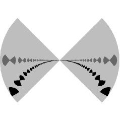
Figure 9. This is a schematic presentation of the values of the complex rotation $\alpha$ where one and two iterates of the top and bottom near-parabolic renormalizations are defined. The light gray region sows the set $A(r_{3})$. The darker gray region is where $\operatorname{{\mathcal{R}}_{\scriptscriptstyle NP-t}^{\circ{2}}}$ and $\operatorname{{\mathcal{R}}_{\scriptscriptstyle NP-b}}\circ\operatorname{{\mathcal{R}}_{\scriptscriptstyle NP-t}}$ are defined. On the black region the iterates $\operatorname{{\mathcal{R}}_{\scriptscriptstyle NP-b}^{\circ{2}}}$ and $\operatorname{{\mathcal{R}}_{\scriptscriptstyle NP-t}}\circ\operatorname{{\mathcal{R}}_{\scriptscriptstyle NP-b}}$ are defined.

When a map is infinitely near-parabolic renormalizable, one may obtain fine scale understanding of the dynamics of that map. For example, for $\kappa$ of constant type $\kappa_{i}=t$ for all $i\geq 1$, this has lead to important properties of the dynamics of quadratic polynomials $Q_{\alpha}$, with irrational $\alpha$ of high type, in [BC12], [Che10b], [Che13], [AC12], and [CC15]. Thus, it is a significant problem to understand when a map is infinitely near-parabolic renormalizable. By virtue of Theorem 2.9, the covering structure of the top and bottom renormalizations of a one time renormalizable map are determined. Thus, the answer to this question relies on controlling the multipliers of the successive renormalizations of the map at the origin.

5.1. Cantor structure in the bifurcation loci

Let $\kappa=(\kappa_{1},\kappa_{2},\kappa_{3},\dots)\in{\mathcal{T}}$, and $r\in(0,r_{3}]$, where $r_{3}$ is the constant obtained in Proposition 2.6. Define $\Lambda_{r}(\kappa_{1})=A(r)$. By Theorem 2.9, for every $f\in\mathcal{I}\mathcal{S}$ and $\alpha\in A(r)$, $\operatorname{\mathcal{R}_{\scriptscriptstyle NP-t}}(\alpha\ltimes f)$ and $\operatorname{\mathcal{R}_{\scriptscriptstyle NP-b}}(\alpha\ltimes f)$ are defined. For integers $n\geq 1$, we consider

(37) $$\Lambda_{r}(\langle\kappa_{i}\rangle_{i=1}^{n})=\Big{\{}\alpha\ltimes f\;\Big{|}\;\begin{array}[]{rr}\operatorname{{\mathcal{R}}_{\scriptscriptstyle NP-\kappa_{n}}}\circ\dots\circ\operatorname{{\mathcal{R}}_{\scriptscriptstyle NP-\kappa_{1}}}(\alpha\ltimes f)\text{ is defined}\\ \text{ and }\forall i\text{ with }1\leq i\leq n,\alpha_{i}\in A(r).\end{array}\Big{\}}.$$

We recall that in the above definition, $\alpha_{i}$ is the rotation number of the map $\operatorname{{\mathcal{R}}_{\scriptscriptstyle NP-\kappa_{i-1}}}\circ\dots\circ\operatorname{{\mathcal{R}}_{\scriptscriptstyle NP-\kappa_{1}}}(\alpha\ltimes f)$ at $0$. In other words, $\Lambda_{r}(\kappa_{1},\dots,\kappa_{n})$ is the set of maps $\alpha\ltimes f$ that are $n$ times near parabolic renormalizable of type $\kappa_{1},\dots,\kappa_{n}$ with the rotation number of all the successive renormalizations in the set $A(r)$. Given $\kappa\in{\mathcal{T}}$, one naturally defines

$$\Lambda_{r}(\kappa)=\bigcap_{n=1}^{\infty}\Lambda_{r}(\langle\kappa_{i}\rangle_{i=1}^{n}).$$

The main result of this paper is stated in the following theorem. We recall that $k_{1}$ and $r_{4}$ are the constant obtained in Proposition 3.1.

Theorem 5.1.

For all $k_{1}$-horizontal family of maps $\Upsilon:A(r_{4})\to{A(r_{4})}\ltimes\mathcal{I}\mathcal{S}$ and all $\kappa\in{\mathcal{T}}$, every connected component of the set $\Lambda_{r_{4}}(\kappa)\cap\Upsilon(A(r_{4}))$ is a single point.

In particular, for all $f\in\mathcal{I}\mathcal{S}\cup\{Q_{0}\}$, and all $\kappa\in{\mathcal{T}}$, every connected component of the set $\Lambda_{r_{4}}(\kappa)\cap(A(r_{4})\ltimes f)$ is a single point.

Proof.

Let $A_{1}$ be a connected component of $\Lambda_{r_{4}}(\kappa)\cap\Upsilon(A(r_{4}))$. By definition, for every $n\geq 1$, every point in $A_{1}$ is near parabolic renormalizable of type $\langle\kappa_{i}\rangle_{i=1}^{k}$. Inductively define the sets $A_{n+1}=\operatorname{{\mathcal{R}}_{\scriptscriptstyle NP-\kappa_{n}}}(A_{n})$, for $n\geq 1$. By Proposition 3.1, each $A_{i}$, $i\geq 1$, is a $k_{1}$-horizontal curves.

Let us define the numbers $\vartheta_{i}$ as the diameter of the projection of the set $A_{i}$ onto the $\alpha$ coordinate. Then, since the diameter of each component of $A(r_{4})$ is equal to $\sqrt{2}r_{4}$, we have $\vartheta_{i}\leq\sqrt{2}r_{4}$. On the other hand, by Proposition  3.3, $\operatorname{\mathcal{R}_{\scriptscriptstyle NP-t}}$ and $\operatorname{\mathcal{R}_{\scriptscriptstyle NP-b}}$ are strictly expanding in horizontal direction. We must have $\vartheta_{i}=0$, for all $i\geq 1$. It follows from the definition of $k_{1}$- horizontal curves that the diameter of each $A_{i}$ must be zero. Indeed, the uniform contraction implies that there are constants $C$ and $\mu\in(0,1)$ such that for all $k_{1}$-horizontal family of maps $\Upsilon:A(r_{4})\to{A(r_{4})}\ltimes\mathcal{I}\mathcal{S}$ and all $\kappa\in{\mathcal{T}}$

$$\operatorname{diam}\,\big{(}\Lambda_{r_{4}}(\langle\kappa_{i}\rangle_{i=1}^{n})\cap\Upsilon(A(r_{4}))\big{)}\leq C\mu^{n}.$$

The latter part of the theorem follows from the first part as the family $\Upsilon(\alpha)=(\alpha,f)$ may be thought of a $0$-horizontal family. ∎

The quadratic polynomial $P_{c}$, with $c\in{\mathbb{C}}$, is conformally conjugate to some $Q_{\alpha(c)}$, with $\operatorname{Re}\alpha(c)\in(-1/2,1/2]$. Indeed, there are two choices for $\alpha(c)$ with this property. The choice does not make any difference for the sake of the next statement, although we will make one of these choices in the next section for our convenience. An immediate corollary of Theorem 5.1 applied to the quadratic family is formulated in the next corollary.

It follows from the proof of the above theorem that the set $\Lambda_{r_{4}}(\kappa)\cap\Upsilon(A(r_{4}))$ is isomorphic to a $\mathcal{I}\mathcal{S}$-bundle over a Cantor set. This is, formulated in the next corollary.

Corollary 5.2.

For all $\kappa\in{\mathcal{T}}$ the restriction of the map $\alpha\ltimes h\mapsto h$ to each connected component of the set $\Lambda_{r_{4}}(\kappa)\cap\Upsilon(A(r_{4}))$ is one-to-one and onto whose image is equal to $\mathcal{I}\mathcal{S}$.

The operators $\operatorname{\mathcal{R}_{\scriptscriptstyle NP-t}}$ and $\operatorname{\mathcal{R}_{\scriptscriptstyle NP-b}}$ map the $\mathcal{I}\mathcal{S}$-fibers of the set $\cup_{\kappa\in{\mathcal{T}}}\Lambda_{r_{4}}(\kappa)\cap\Upsilon(A(r_{4}))$ to the fibers. Combining with the uniform contraction in Theorem 2.9, we obtain the uniform contraction of the operators $\operatorname{\mathcal{R}_{\scriptscriptstyle NP-t}}$ and $\operatorname{\mathcal{R}_{\scriptscriptstyle NP-b}}$ on the co-dimension one fibers.

Corollary 5.3.

Let $\langle p_{i}/q_{i}\rangle_{i=1}^{\infty}$ be a sequence of rational numbers in $(-1/2,1/2]$ and $\kappa\in{\mathcal{T}}$ be a type such that for all $c\in M(\langle p_{i}/q_{i}\rangle_{i=1}^{\infty})$, $Q_{\alpha(c)}$ is infinitely near parabolic renormalizable of type $\kappa$ and for every $i\geq 1$ the rotation number $\alpha_{i}$ of the $i$-th renormalization of $Q_{\alpha(c)}$ belongs to $A(r_{4})$. Then, the nest of Mandelbrot copies $M(\langle p_{i}/q_{i}\rangle_{i=1}^{n})$ shrinks (geometrically) to a single point as $n$ tends to infinity.

Although in the above corollary the sequence of rational numbers and the type $\kappa$ are not related apriori, in Section 6.3 we associate a canonic type $\kappa$ to any given sequence of rational numbers in $(-1/2,1/2]$.

6. Application to the complex quadratic polynomials

6.1. Modified continued fractions

We work with a modified notion of continued fractions that is more suitable in the study of the near-parabolic renormalization.

For $x\in{\mathbb{R}}$, let $[x]$ denote the closest integer to $x$, where we use the convention

$$x\in([x]-1/2,[x]+1/2],\text{for }x>0,$$

$$x\in[[x]-1/2,[x]+1/2),\text{for }x<0.$$

We have adapted the above convention to obtain a $x\mapsto-x$ symmetry in the continued fraction expansion introduced below.

Let $x\in[-1/2,1/2]\setminus\{0\}$ be a rational number and set $x_{1}=x$. There is a positive integer $n$ such that the numbers

(38) $$[x_{i+1}]=\frac{-1}{x_{i}}-\left[\frac{-1}{x_{i}}\right],1\leq i\leq n,$$

are defined and $x_{n+1}=0$. For $1\leq i\leq n$, we define the signs $\varepsilon_{i}^{\prime}=+1$ if $x_{i}>0$ and $\varepsilon^{\prime}_{i}=-1$ if $x_{i}<0$, and then define the integers $b_{i}\geq 2$ according to

$$b_{i}=\begin{cases}\big{[}\frac{-1}{x_{i}}\big{]}&\text{if }\varepsilon^{\prime}_{i}=-1,\\ \big{[}\frac{1}{x_{i}}\big{]}&\text{if }\varepsilon^{\prime}_{i}=+1.\end{cases}$$

It follows that $[-1/x_{i}]=\varepsilon^{\prime}_{i}b_{i}$, and hence $x_{i}^{-1}=\varepsilon^{\prime}_{i}b_{i}-x_{i+1}$. Now let us define the signs $\varepsilon_{1}=\varepsilon_{1}^{\prime}$, and $\varepsilon_{i}=(-1)\varepsilon^{\prime}_{i-1}\varepsilon^{\prime}_{i}$, for $2\leq i\leq n$. Then, one can see that $x$ is given by the finite continued fraction

$$x=x_{1} =1/(\varepsilon^{\prime}_{1}b_{1}-x_{2})=\varepsilon_{1}/(b_{1}-\varepsilon_{1}^{\prime}x_{2}),$$

$$=\cfrac{\varepsilon_{1}}{b_{1}-\varepsilon^{\prime}_{1}\cfrac{1}{\varepsilon^{\prime}_{2}b_{2}-x_{3}}}=\cfrac{\varepsilon_{1}}{b_{1}+\cfrac{-1\varepsilon_{1}^{\prime}\varepsilon_{2}^{\prime}}{b_{2}-\varepsilon_{2}^{\prime}x_{3}}}=\cfrac{\varepsilon_{1}}{b_{1}+\cfrac{\varepsilon_{2}}{b_{2}-\varepsilon_{2}^{\prime}x_{3}}}.$$

Inductively, repeating the above process until $x_{n+1}=0$, we obtain

$$x=\cfrac{\varepsilon_{1}}{b_{1}+\cfrac{\varepsilon_{2}}{\ddots+\cfrac{\varepsilon_{n}}{b_{n}}}}.$$

Remark 6.1.

The above continued fraction expansion is slightly different from the usual notion of modified (closest integer) continued fraction expansion in the literature, where we use $x-[x]$ instead of $d(x,{\mathbb{Z}})$ and allow $x_{i}$ to be negative as well as positive. However, the only difference between the two expansions is in the signs $\varepsilon_{i}$. The reason for adapting to the above algorithm is that we shall later extend the map $x\mapsto x-[x]$ to a holomorphic map on a neighborhood of the interval $[-1/2,1/2]$. This allows us to study the maps $\alpha\mapsto\operatorname{\mathcal{R}_{\scriptscriptstyle NP-t}}(\alpha\ltimes f)$ and $\alpha\mapsto\operatorname{\mathcal{R}_{\scriptscriptstyle NP-b}}(\alpha\ltimes f)$ as holomorphic maps of $\alpha$ rather than anti-holomorphic maps of $\alpha$.

Given $n\geq 1$ and a sequence of pairs $\langle b_{i}:\varepsilon_{i}\rangle_{i=1}^{n}$, where each $b_{i}\geq 2$ is an integer and $\varepsilon_{i}\in\{+1,-1\}$, we use the notation $[\langle b_{i}:\varepsilon_{i}\rangle_{i=1}^{n}]$ to denote the rational number generated by this sequence of pairs. That is,

$$[b_{1}:\varepsilon_{1}]=\frac{\varepsilon_{1}}{b_{1}},\quad[(b_{1}:\varepsilon_{1}),(b_{2}:\varepsilon_{2})]=\cfrac{\varepsilon_{1}}{b_{1}+\cfrac{\varepsilon_{2}}{b_{2}}},$$

and for $n\geq 3$,

$$[\langle b_{i}:\varepsilon_{i}\rangle_{i=1}^{n}]=\cfrac{\varepsilon_{1}}{b_{1}+\cfrac{\varepsilon_{2}}{\ddots+\cfrac{\varepsilon_{n}}{b_{n}}}}.$$

However, note that a rational number of the above form is not necessarily in the interval $[-1/2,1/2]$. But, it is fairly close. The only condition we need to impose to obtain a rational number in the interval $[-1/2,1/2]$ is that when $b_{1}=2$ we must have $\varepsilon_{1}\varepsilon_{2}=+1$.

6.2. Sequences of rational numbers

Let $n\geq 1$ be an integer, and let $m_{i}\geq 1$ and $b_{i,j}\geq 2$ be integers, and $\varepsilon_{i,j}\in\{+1,-1\}$, for $1\leq i\leq n$ and $1\leq j\leq m_{i}$. We define the notation

$$\langle m_{i}:b_{i,j}:\varepsilon_{i,j}\rangle_{i=1}^{n}$$

to represent the finite sequence of rational numbers

$$\langle[b_{i,j}:\varepsilon_{i,j}]_{j=1}^{m_{i}}\rangle_{i=1}^{n}$$

For each $i$ and $l$ with $1\leq i\leq n$ and $1\leq l\leq m_{i}$ we let

$$\frac{p_{i,l}}{q_{i,l}}=[\langle b_{i,j}:\varepsilon_{i,j}\rangle_{j=1}^{l}].$$

Thus,

$$\langle m_{i}:b_{i,j}:\varepsilon_{i,j}\rangle_{i=1}^{n}=\langle\frac{p_{i,m_{i}}}{q_{i,m_{i}}}\rangle_{i=1}^{n}.$$

Although we may remove the second subscript $m_{i}$ from the numerator and denominator of the above sequence to get the simpler notation $p_{i}/q_{i}=p_{i,m_{i}}/q_{i,m_{i}}$, these have been put there to avoid possible future confusions that the sequence $p_{i}/q_{i}$ forms the fractions of a single number. That is, a priori there is no relation between these fractions. When we are interested in infinite sequences of rational numbers, we shortened the notation $\langle m_{i}:b_{i,j}:\varepsilon_{i,j}\rangle_{i=1}^{\infty}$ to $\langle m_{i}:b_{i,j}:\varepsilon_{i,j}\rangle$.

By setting the initial data $p_{i,-1}=q_{i,0}=1$ and $p_{i,0}=q_{i,-1}=0$, we have the usual recursive formulas for the continued fractions $p_{i,l}/q_{i,l}$, $0\leq l\leq m_{i}$

$$q_{i,l+1}=b_{i,l+1}q_{i,l}+\varepsilon_{i,l}q_{i,l-1},\quad p_{i,l+1}=b_{i,l+1}p_{i,l}+\varepsilon_{i,l}p_{i,l-1},$$

By an inductive process, the above formulas imply that for all $i\geq 1,0\leq l\leq m_{i}-1$, we have

(39) $$q_{i,l+1}>q_{i,l}.$$

Moreover, for every $i\geq 1$,

(40) $$\frac{1}{q_{i,m_{i}}}=\Big{|}\prod_{k=1}^{m_{i}}[\langle b_{i,j}:\varepsilon_{i,j}\rangle_{j=k}^{m_{i}}]\Big{|}.$$

6.3. Pairs of multipliers vs pairs of complex rotations

Let $\kappa=(\kappa_{1},\kappa_{2},\kappa_{3},\dots)$ be in ${\mathcal{T}}$, where the set of types ${\mathcal{T}}$ is defined in Equation (33). In analogy with the set $\Lambda_{r}(\kappa_{1},\dots,\kappa_{n})$ defined in Equation (37), we consider the sets

$$\Lambda_{r}^{1}(\langle\kappa_{i}\rangle_{i=1}^{n})=\Big{\{}\alpha\in A(r_{3})\Big{|}\begin{array}[]{rr}\operatorname{{\mathcal{R}}_{\scriptscriptstyle NP-\kappa_{n}}}\circ\dots\circ\operatorname{{\mathcal{R}}_{\scriptscriptstyle NP-\kappa_{1}}}(Q_{\alpha})\text{ is defined}\\ \text{ and }\forall i\text{ with }1\leq i\leq n,\alpha_{i}\in A(r).\end{array}\Big{\}}$$

For example, by Theorem 2.9, $\operatorname{\mathcal{R}_{\scriptscriptstyle NP-t}}(Q_{\alpha})$ and $\operatorname{\mathcal{R}_{\scriptscriptstyle NP-b}}(Q_{\alpha})$ are defined for $\alpha\in\Lambda_{r_{3}}^{Q}(\kappa_{1})$.

Each $Q_{\alpha}$ with $\alpha\in{\mathbb{C}}$ is conformally conjugate to some quadratic polynomial $P_{c}$ with a unique $c\in{\mathbb{C}}$. The connectedness locus of the family $Q_{\alpha}$, that is, the set of $\alpha$ such that the Julia set of $Q_{\alpha}$ is connected, is ${\mathbb{Z}}$-periodic in $\alpha$. However, this connectedness locus modulo ${\mathbb{Z}}$ forms a double cover of the Mandelbrot set, branched over $c=1/4$ (which is only covered once). Here $\alpha=0$ is mapped to $c=1/4$. For each $c\in{\mathbb{C}}\setminus\{1/4\}$ there are two distinct parameters $w_{1}$ and $w_{2}$ in ${\mathbb{C}}$ such that for all $\alpha$ in $w_{1}+{\mathbb{Z}}$ and $w_{2}+{\mathbb{Z}}$, $Q_{\alpha}$ is conformaly conjugate to $P_{c}$. See Figure 10.

For $\alpha$ in the upper half plane, $0$ is an attracting fixed point of $Q_{\alpha}$, while for $\alpha$ in ${\mathbb{R}}$ the multiplier of $Q_{\alpha}$ at $0$ belongs to the unit circle. In analogy to the Mandelbrot set, the connectedness locus of $Q_{\alpha}$ minus ${\mathbb{R}}$ consists of the upper half plane and the connected components attached to the real line at rational values of $\alpha$. There is a unique connected component attached to the real line at $0$. We denote the closure of this component by $M_{\alpha}$. Then, there is a one-to-one correspondence between the Mandelbrot set and $M_{\alpha}$ such that the corersponding quadratic polynomials are conformally conjugate. Let $c\mapsto\alpha(c)$, from $M$ to $M_{\alpha}$, denote this bijection. We define the sets

$$M_{\alpha}(\big{\langle}\frac{p_{i}}{q_{i}}\big{\rangle}_{i=1}^{n})=\big{\{}\alpha(c)\mid c\in M(\big{\langle}\frac{p_{i}}{q_{i}}\big{\rangle}_{i=1}^{n})\big{\}}.$$

As in Section 4, the notions of dividing periodic points and their combinatorial rotation numbers are defined on the above components.

      

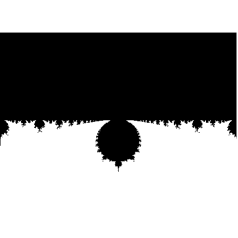
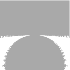
Figure 10. The connectedness locus of the family $Q_{\alpha}$ and a zoom into a neighborhood of $0$ on the right hand side. Need to produce better figures.

Let $Q_{\alpha}$ be an infinitely polynomial-like renormalizable. We denote the sequence of the dividing periodic points of $Q_{\alpha}$ by $\nu_{i}$, $i\geq 1$. In other words, $\nu_{i}$ in the periodic point of $Q_{\alpha}$ that is mapped to $a_{i}$ by the conformal map conjugating $Q_{\alpha(c)}$ to $P_{c}$, for each $i\geq 1$. We recall that $\nu_{1}$ is a fixed point. Note that $\nu_{i}$ is not an arbitrary element in the cycle of $\nu_{i}$. Rather, it is a particular point in this cycle. Let us denote the multiplier of $\nu_{i}$ by $\rho_{i}$, for $i\geq 1$. That is,

$$\rho_{1}=Q_{\alpha}^{\prime}(\nu_{1}),\;\rho_{2}=(Q_{\alpha}^{\circ{q_{1}}})^{\prime}(\nu_{2}),\;\rho_{n}=(Q_{\alpha}^{\circ{(q_{1}\dots q_{n-1})}})^{\prime}(\nu_{n}),n\geq 3.$$

For $\alpha\in M_{\alpha}\setminus\{0\}$, $0$ is a repelling fixed point of $Q_{\alpha}$ while $\sigma(Q_{\alpha})$ may be either attracting or repelling, depending on $\operatorname{Im}(\beta(Q_{\alpha}))$. For $\alpha\in M_{\alpha}\setminus\{0\}$, $\nu_{1}=\sigma_{1}=\sigma(Q_{\alpha})$ is the non-zero fixed point of $Q_{\alpha}$, and we have

(41) $$\beta_{1}=\frac{1}{2\pi\textnormal{{i}}}\log\rho_{1}.$$

Let $p_{i}/q_{i}$ be a sequence of non-zero rational numbers in $(-1/2,1/2]$. By the previous section, there is $\langle m_{i}:b_{i,j}:\varepsilon_{i,j}\rangle_{i=1}^{\infty}$, with integers $m_{i}\geq 1$, $b_{i,j}\geq 2$, and signs $\varepsilon_{i,j}$ for $i\geq 1$ and $1\leq j\leq m_{i}$, such that $p_{i}/q_{i}=p_{i,m_{i}}/q_{i,m_{i}}=[\langle b_{i,j}:\varepsilon_{i,j}\rangle_{i=1}^{m_{i}}]$, for $i\geq 1$. Then, we consider the integers

(42) $$l_{1}=0,\;l_{k}=\sum_{i=1}^{k-1}m_{i},k\geq 1.$$

Then, we define the map

(43) $$\kappa:\big{(}{\mathbb{Q}}\cap\big{(}(-1/2,0)\cup(0,1/2]\big{)}\big{)}^{\mathbb{N}}\to{\mathcal{T}},$$

as follows. Given $\langle m_{i}:b_{i,j}:\varepsilon_{i,j}\rangle$ in $\big{(}{\mathbb{Q}}\cap\big{(}(-1/2,0)\cup(0,1/2]\big{)}\big{)}^{\mathbb{N}}$ and $n\geq 1$, the $n$-th entry of $\kappa(\langle m_{i}:b_{i,j}:\varepsilon_{i,j}\rangle)$, denoted by $\kappa_{n}(\langle m_{i}:b_{i,j}:\varepsilon_{i,j}\rangle)$, is defined as

$$\kappa_{n}(\langle m_{i}:b_{i,j}:\varepsilon_{i,j}\rangle)=\begin{cases}b&\text{if }n\in\{l_{k}+1\mid k\geq 1\}\\ t&\text{ otherwise.}\end{cases}$$

In other words, the first $m_{1}$ entries of $\kappa$ are given by one “b” followed by $m_{1}-1$ times “t”, the next $m_{2}$ entries of $\kappa$ are given by one “b” followed by $m_{2}-1$ times “t”, and so on. The map $\kappa$ only depends on the sequence $m_{i}$ (the lengths of the rational numbers) rather than the entries in each rational number. The individual entries come into play later.

In the following proposition $r_{3}$ denotes the constant introduced in Proposition 2.6.

Proposition 6.2.

Let $\langle p_{i}/q_{i}\rangle_{i=1}^{\infty}=\langle m_{i}:b_{i,j}:\varepsilon_{i,j}\rangle$ be a sequence of non-zero rational numbers in $(-1/2,1/2]$ and consider the type $\kappa=\kappa(\langle m_{i}:b_{i,j}:\varepsilon_{i,j}\rangle)\in{\mathcal{T}}$. For every integer $k\geq 0$ and every $\alpha$ in the intersection of $M_{\alpha}(\langle p_{i}/q_{i}\rangle_{i=1}^{k})$ and $\Lambda_{r_{3}}^{1}(\kappa_{1},\dots,\kappa_{l_{k}})$, if $\alpha_{l_{k}+1}\in A(r_{3})$ then

$$\beta_{l_{k}+1}=\frac{1}{2\pi\textnormal{{{i}}}}\log\rho_{k}.$$

Proof.

Since $\alpha\in M_{\alpha}(p_{1}/q_{1},\dots,p_{k}/q_{k})$, for every integer $j$ with $1\leq j\leq k$ the dividing periodic point $\nu_{j}$ of $Q_{\alpha}$ is defined. In particular, the right hand side of the equality in the proposition is defined. On the other hand, as $\alpha\in\Lambda(\kappa_{1},\dots,\kappa_{l_{k}})$, for every integer $j$ with $2\leq j\leq l_{k}$ $f_{j+1}=\operatorname{{\mathcal{R}}_{\scriptscriptstyle NP-\kappa_{j}}}\circ\dots\circ\operatorname{{\mathcal{R}}_{\scriptscriptstyle NP-\kappa_{1}}}(Q_{\alpha})$ is defined. Moreover, by the definition of $\Lambda(\kappa_{1},\dots,\kappa_{l_{k}})$ and the assumption in the proposition for every $1\leq j\leq l_{k}+1$, $\alpha_{j}$ is defined and belongs to $A(r_{3})$. By Proposition 2.1, this implies that each $f_{j}$ has a unique non-zero fixed point $\sigma_{j}$ in the (fixed) neighborhood $W$ of $0$. In particular, $\beta_{l_{k}+1}$ in the left-hand side of the equation in the proposition is defined. It remains to relate these quantities.

Recall that for $\alpha\in M_{\alpha}(p_{1}/q_{1},\dots,p_{k}/q_{k})$, $\nu_{1}$ is a fixed point, and in general for $j$ with $2\leq j\leq k$, $\nu_{j}$ is a periodic point of period $\prod_{i=1}^{j-1}q_{i}$. Moreover, as $\alpha$ varies in $M_{\alpha}(p_{1}/q_{1},\dots,p_{j}/q_{j})$, $\nu_{j}$ has holomorphic dependence on $\alpha$. On the other hand, by the definition of the near-parabolic renormalizations, each $\sigma_{l_{j}+1}$, for $1\leq j\leq k$, lifts to a periodic cycle of $Q_{\alpha}$, which we denote by $O_{l_{j}+1}$. We claim that for each $j$ with $1\leq j\leq k$, $O_{l_{j}+1}$ is equal to the cycle of $\nu_{j}$. We prove this below by induction on $j$.

For $j=1$, $l_{1}=0$ and $O_{1}$ is equal to $\sigma_{1}=\sigma(Q_{\alpha})=\nu_{1}$. Assume that $O_{l_{j-1}+1}$ is equal to the cycle of $\nu_{j-1}$ for $j-1<l+1$ and we want to prove that $O_{l_{j}+1}$ is equal to the cycle of $\nu_{j}$. By the definition of the types, $\kappa_{l_{j-1}+1}=b$ and for all integers $i$ with $l_{j-1}+1<i\leq l_{j}$, we have $\kappa_{i}=t$. This implies that the zero fixed point of $f_{l_{j}+1}$ lifts to $\sigma_{l_{j-1}+1}$ on the dynamic pane of $f_{l_{j-1}+1}$ (in all the intermediate levels $i$ it lifts to $0$). Thus, by the induction hypothesis, the zero fixed point of $f_{l_{j}+1}$ lifts to the cycle of $\nu_{j-1}$. On the other hand, as $\alpha_{l_{j}+1}$ tends to $0$ in $A(r_{3})$, $\sigma_{l_{j}+1}$ tends to $0$ and $\sigma_{l_{j}+1}$ is the only fixed point of $f_{l_{j}+1}$ within $W$-neighborhood of $0$. This implies that the lift of this fixed point, which is the cycle $O_{l_{j}+1}$, tends to the cycle of $\nu_{j-1}$. However, as $\alpha\in M(p_{1}/q_{1},\dots,p_{j}/q_{j})$, $\nu_{j}$ is the only periodic point of $Q_{\alpha}$ that bifurcates from $\nu_{j-1}$. That is, for sufficiently small $\alpha_{l_{j}+1}$ (equivalently, for $\alpha$ sufficiently close to the root point of $M(p_{1}/q_{1},\dots,p_{j}/q_{j})$), $O_{l_{j}+1}$ is equal to the cycle of $\nu_{j}$. By the holomorphic dependence of the cycles of $\nu_{j}$ and $O_{l_{j}+1}$ on $\alpha$, we conclude that these cycles are equal on the connected components of $\Lambda(\kappa_{1},\dots,\kappa_{l_{j}})$.

By the above argument, $\sigma_{l_{k}+1}$ lifts to the orbit of $\nu_{k}$ through the changes of the coordinates in the near-parabolic renormalizations. In particular, these cycles must have the same multipliers, as in the equation in the proposition. ∎

Corollary 6.3.

Let $\langle m_{i}:b_{i,j}:\varepsilon_{i,j}\rangle$ be a sequence of non-zero rational numbers in $(-1/2,1/2]$. For every $\alpha$ in the intersection of $M_{\alpha}(\langle m_{i}:b_{i,j}:\varepsilon_{i,j}\rangle)$ and $\Lambda_{r_{3}}^{1}(\kappa(\langle m_{i}:b_{i,j}:\varepsilon_{i,j}\rangle))$, and every $k\geq 1$ we have

$$\beta_{l_{k}+1}=\frac{1}{2\pi\textnormal{{{i}}}}\log\rho_{k}.$$

6.4. The quadratic growth condition and the complex rotations

Here, our goal is to find a combinatorial condition, in terms of the combinatorial rotation numbers of the dividing periodic points, that guarantees an infinitely polynomial-like renormalizable map under that condition is infinitely near-parabolic renormalizable.

The algorithm defining the modified continued fraction expansion in Section 6.1 has a natural extension onto the complex plane which plays a crucial role in this section. It is defined as follows. Recall from Section 6.1 the closest integer function $[\cdot]$ defined on ${\mathbb{R}}$. We consider the map $\operatorname{inv}(z)=-1/z$, for $z\in{\mathbb{C}}\setminus\{0\}$, and the map $\operatorname{saw}(z)=z-[\operatorname{Re}(z)]$, for $z\in{\mathbb{C}}$. We shall work with the composition of these two maps denote by

$$G(z)=\operatorname{saw}\circ\operatorname{inv}(z),\forall z\in{\mathbb{C}}\setminus\{0\}.$$

Then, $G$ maps the interval $[-1/2,0)\cup(0,1/2]$ to $[-1/2,1/2]$, and for a non-zero rational number in $x_{1}$ in $[-1/2,1/2]$,

$$x_{i}=G^{\circ{i-1}}(x_{1}),1\leq i\leq n.$$

where the numbers $x_{i}$ are defined in Equation (38). In particular,

$$G([\langle b_{j}:\varepsilon_{j}\rangle_{j=i}^{n}])=-\varepsilon_{1}\cdot[\langle b_{j}:\varepsilon_{j}\rangle_{j=i+1}^{n}].$$

That is, applying $G$ to a continued fraction, removes the first pair from the expansion, and then only modifies the first sign in the remaining expansion. In particular,

$$G^{\circ{n-1}}([\langle b_{j}:\varepsilon_{j}\rangle_{j=1}^{n}])=\pm 1/b_{n},\;G^{\circ{n}}([\langle b_{j}:\varepsilon_{j}\rangle_{j=1}^{n}])=0.$$

For each integer $b_{1}\geq 2$ and $\varepsilon_{1}\in\{+1,-1\}$, the image of the round ball of radius $1/2$ centered at $-\varepsilon_{1}b_{1}$, $B(-\varepsilon_{1}b_{1},1/2)$, under the map $\operatorname{inv}$ is a round ball containing $\varepsilon_{1}/b_{1}$. Note that this ball is not centered at $\varepsilon_{1}/b_{1}$. Let ${\mathcal{F}}_{1}$ denote the collection of all these balls for integers $b_{1}\geq 2$ and $\varepsilon_{1}\in\{+1,-1\}$. If we care to determine a specific ball in this collection, we use the notation ${\mathcal{F}}_{1}(\langle b_{1}:\varepsilon_{1}\rangle)$ to denote the one containing $\varepsilon_{1}/b_{1}$. It follows that $G:{\mathcal{F}}_{1}(\langle b_{1}:\varepsilon_{1}\rangle)\to B(0,1/2)$ is a holomorphic bijection.

Similarly, for integers $n\geq 2$, we may define the collection ${\mathcal{F}}_{n}$ of round balls that are mapped onto $B(0,1/2)$ by the iterate $G^{\circ{n}}$. The element of ${\mathcal{F}}_{n}$ containing $[\langle b_{1}:\varepsilon_{1}\rangle_{i=1}^{n}]$ is denoted by ${\mathcal{F}}_{n}(\langle b_{i}:\varepsilon_{i}\rangle_{i=1}^{n})$ and we note that each such element is a disk that is symmetric with respect to the real line. Moreover,

$$G^{\circ{n}}:{\mathcal{F}}_{n}([\langle b_{i}:\varepsilon_{i}\rangle_{i=1}^{n}])\to B(0,1/2),n\geq 1,$$

is a holomorphic bijection given by a Möbius transformation that maps the real slice of the domain to the real slice of the image.

Lemma 6.4.

For every $n\geq 1$, every $[\langle b_{j}:\varepsilon_{j}\rangle_{j=1}^{n}]\in{\mathbb{Q}}$, every $z\in{\mathcal{F}}_{n}([\langle b_{j}:\varepsilon_{j}\rangle_{j=1}^{n}])$, and every $k$ with $0\leq k\leq n-1$, we have

$$\frac{4}{5}\cdot\frac{1}{b_{k+1}}\leq|G^{\circ{k}}(z)|\leq\frac{4}{3}\cdot\frac{1}{b_{k+1}},\quad\arg G^{\circ{k}}(z)\in\begin{cases}[\frac{-\pi}{4},\frac{\pi}{4}]&\text{if }\operatorname{Re}(G^{\circ{k}}(z))>0\\ [\frac{3\pi}{4},\frac{5\pi}{4}]&\text{if }\operatorname{Re}(G^{\circ{k}}(z))<0\end{cases}.$$

Proof.

First note that

$$G^{\circ{k}}\big{(}{\mathcal{F}}_{n}([\langle b_{j}:\varepsilon_{j}\rangle_{j=1}^{n}]\big{)}={\mathcal{F}}_{n-k}(G^{\circ{k}}([\langle b_{j}:\varepsilon_{j}\rangle_{j=1}^{n}])\subseteq{\mathcal{F}}_{1}(G^{\circ{k}}([\langle b_{j}:\varepsilon_{j}\rangle_{j=1}^{n}]).$$

and the first pair in the expansion of $G^{\circ{k}}([\langle b_{j}:\varepsilon_{j}\rangle_{j=1}^{n}]$ has the form $(b_{k+1},\pm 1)$. Hence, $G^{\circ{k}}(z)$ belongs to either ${\mathcal{F}}_{1}(1/b_{k+1})$ or ${\mathcal{F}}_{1}(-1/b_{k+1})$. Each of these sets is a round ball symmetric with respect to the real line passing through the pair of points $1/(b_{k+1}+1/2)$ and $1/(b_{k+1}-1/2)$ or the pair of points $-1/(b_{k+1}+1/2)$ and $-1/(b_{k+1}-1/2)$, respectively. In particular, for $G^{\circ{k}}(z)\in{\mathcal{F}}_{1}(\pm 1/b_{k+1})$,

$$\frac{4}{5}\cdot\frac{1}{b_{k+1}}\leq\frac{1}{b_{k+1}+1/2}\leq|z|\leq\frac{1}{(b_{k+1}-1/2)}\leq\frac{4}{3}\cdot\frac{1}{b_{k+1}}.$$

On the other hand, each of ${\mathcal{F}}_{1}(1/b_{k+1})$ and ${\mathcal{F}}_{1}(-1/b_{k+1})$ is a round disk of diameter

$$\frac{1}{b_{k+1}-1/2}-\frac{1}{b_{k+1}+1/2}\leq\frac{1}{\sqrt{2}b_{k+1}}.$$

Hence, ${\mathcal{F}}_{1}(\pm 1/b_{k+1})$ is contained in the round ball of radius $1/(\sqrt{2}b_{k+1})$ about $\pm 1/b_{k+1}$. This implies the bounds on $\arg(G^{\circ{k}}(z))$. ∎

Lemma 6.5.

There is a constant $C_{0}$ satisfying the following. Let $x=[\langle b_{j}:\varepsilon_{j}\rangle_{j=1}^{n}]\in{\mathbb{Q}}$, for some $n\geq 1$, and assume that $b_{j+1}\geq b_{j}^{2}$, for $1\leq j\leq n-1$. Define the numbers

$$x_{0}=1,x_{i}=G^{\circ{(i-1)}}(x),\quad 1\leq i\leq n.$$

Then,

$$\frac{|x_{n}|}{|x_{1}|}\leq C_{0}\cdot\prod_{i=0}^{n-1}|x_{i}|.$$

Proof.

For each $1\leq j\leq n$ we have

$$\big{(}1+\frac{1}{2b_{j}+1}\big{)}\frac{1}{b_{j}}=\frac{1}{b_{j}+1/2}\leq|x_{j}|\leq\frac{1}{b_{j}-1/2}=\frac{1}{b_{j}}\cdot\big{(}1+\frac{1}{2b_{j}-1}\big{)}.$$

Then, since $b_{j+1}\geq b_{j}^{2}$, by the above equation we have

$$|x_{j+1}|\leq\frac{1}{b_{j+1}}\big{(}1+\frac{1}{2b_{j+1}-1}\big{)}\\ \leq\frac{1}{b_{j}^{2}}\big{(}1+\frac{1}{2b_{j+1}-1}\big{)}\leq|x_{j}|^{2}\big{(}1+\frac{1}{2b_{j+1}-1}\big{)}\big{(}1-\frac{1}{2b_{j}+2}\big{)}^{2}\\ \leq|x_{j}|^{2}(1+\frac{C}{b_{j}}),$$

For some uniform constant $C$. Then,

$$\frac{|x_{n}|}{\prod_{i=0}^{n-1}|x_{i}|}=\prod_{i=0}^{n-1}\big{(}\frac{|x_{i+1}|}{|x_{i}|^{2}}\big{)}\leq|x_{1}|\big{(}\prod_{i=1}^{n-1}(1+\frac{C}{b_{i}})\big{)}\leq|x_{1}|\exp(\sum_{i=1}^{\infty}\frac{C}{b_{i}})\leq|x_{1}|e^{C}.$$

∎

Lemma 6.6.

There exists $C_{1}>0$ such that for every $n\geq 1$ and every disk $B_{n}$ in ${\mathcal{F}}_{n}$, the distortion of the map $G^{\circ{n}}:B_{n}\to B(0,1/2)$ is bounded by $C_{1}$, that is,

$$\forall z,w\in B_{n},\frac{1}{C_{1}}\leq\Big{|}\frac{(G^{\circ{n}})^{\prime}(z)}{(G^{\circ{n}})^{\prime}(w)}\Big{|}\leq C_{1}.$$

Proof.

Assume that $B$ and $B^{\prime}$ are round disks that are symmetric with respect to the real line (invariant under complex conjugation), and $g:B\to B^{\prime}$ be a Möbius map that sends $B\cap{\mathbb{R}}$ to $B^{\prime}\cap{\mathbb{R}}$. Then, the distortion of $g$ on $B$ is realized at the two end points of the interval $B\cap{\mathbb{R}}$. This implies that the distortion of the map $G^{\circ{n}}$ on $B_{n}$ is equal to its distortion on $B_{n}\cap{\mathbb{R}}$. Indeed, the latter statement is a classical result that follows from direct calculations. ∎

Let $N\geq 2$ be an integer and define the class of sequences of rational numbers

(44) $${\mathcal{QG}}_{N}=\Big{\{}\big{\langle}\frac{p_{i,m_{i}}}{q_{i,m_{i}}})\big{\rangle}_{i=1}^{\infty}=\langle m_{i}:b_{i,j}:\varepsilon_{i,j}\rangle\Big{|}\begin{array}[]{l}b_{1,1}\geq N;\forall i\geq 1,b_{i+1,1}\geq q_{i,m_{i}}^{2}\\ \forall i\geq 1,1\leq j\leq m_{i}-1,b_{i,j+1}\geq b_{i,j}^{2}.\end{array}\Big{\}}.$$

For example, if we let $m_{i}=1$ for all $i\geq 1$, then a sequence $\langle p_{i,1}/q_{i,1}\rangle_{i=1}^{\infty}$ belongs to ${\mathcal{QG}}_{N}$ if and only if $q_{1}\geq N$ and for all $i\geq 1$, $p_{i}\in\{+1,-1\}$ and $q_{i+1}\geq q_{i}^{2}$. However, choosing larger values of $m_{i}$ at different stages allows us to cover more rational number at stage $i$. This imposes a stronger condition on the size of the next denominator through $q_{i+1}\geq b_{i,m_{i}}^{2}$.

Proposition 6.7.

For every $r\in(0,1/2)$ there is a constant $N>0$ satisfying the following property. Let $\langle p_{i}/q_{i}\rangle_{i=1}^{\infty}$ belong to ${\mathcal{QG}}_{N}$ and define the integers

$$k_{1}=1,k_{n}=\prod_{i=1}^{n-1}q_{i,m_{i}},\forall i\geq 1.$$

Then, for every $i\geq 1$ and every $z\in{\mathbb{C}}$ satisfying

$$\Big{|}z-\big{(}\frac{p_{i}}{q_{i}}-\textnormal{{{i}}}\frac{k_{i}}{q_{i}}\frac{\log 2}{2\pi}\big{)}\Big{|}\leq\frac{\log 2}{2\pi}\frac{k_{i}}{q_{i}},$$

we have the following two properties.

• For every $n_{i}$ with $0\leq n_{i}\leq m_{i}-2$,

  $$|G^{\circ{n_{i}}}(z)|\leq r,\text{ and }\arg(G^{\circ{n_{i}}}(z))\in\begin{cases}[-\frac{\pi}{4},\frac{\pi}{4}]&\text{if }\operatorname{Re}(G^{\circ{n_{i}}}(z))>0\\ [\frac{3\pi}{4},\frac{5\pi}{4}]&\text{if }\operatorname{Re}(G^{\circ{n_{i}}}(z))<0\end{cases};$$

• $$|G^{\circ{(m_{i}-1)}}(z)|\leq r.$$

Proof.

Let us choose $\langle m_{i}:b_{i,j}:\varepsilon_{i,j}\rangle$ so that

$$\frac{p_{i}}{q_{i}}=\frac{p_{i,m_{i}}}{q_{i,m_{i}}}=[\langle b_{i,j}:\varepsilon_{i,j}\rangle_{j=1}^{m_{i}}].$$

Recall the constants $C_{0}$ and $C_{1}$ introduced in Lemmas 6.5 and 6.6. Then, choose $N\geq 2$ such that the following inequalities hold.

(45) $$\frac{1}{N}\frac{4}{3}\leq\frac{r}{2},$$

(46) $$\frac{1}{N}\frac{4}{3}C_{1}\leq\frac{1}{C_{1}}\cdot\frac{\sqrt{C_{1}}-1}{\sqrt{C_{1}}+1}\cdot\frac{r}{2},$$

(47) $$\frac{1}{N}C_{1}\frac{4}{3}\frac{\log 2}{2\pi}\frac{5}{4}C_{1}C_{0}\leq\frac{1}{C_{1}}\cdot\frac{\sqrt{C_{1}}-1}{\sqrt{C_{1}}+1}\cdot\frac{r}{2}$$

We break the proof into several steps.

Step 1. For $\langle m_{i}:b_{i,j}:\varepsilon_{i,j}\rangle\in{\mathcal{QG}}_{N}$, by Lemma 6.4, for every $i\geq 1$ and every $n_{i}$ with $0\leq n_{i}\leq m_{i}-1$, by Equation (45), we have

(48) $$\big{|}G^{\circ{n_{i}}}\big{(}[\langle b_{i,j}:\varepsilon_{i,j}\rangle_{j=1}^{m_{i}}]\big{)}\big{|}\leq\frac{4}{3}\cdot\frac{1}{b_{i,n_{i}+1}}\leq\frac{4}{3}\cdot\frac{1}{b_{i,1}}\leq\frac{4}{3}\cdot\frac{1}{b_{1,1}}\leq\frac{4}{3}\cdot\frac{1}{N}\leq\frac{r}{2}.$$

Step 2. By the definition of the class ${\mathcal{QG}}_{N}$ and Equation (39), for every $i\geq 1$,

(49) $$q_{i+1,m_{i+1}}\geq q_{i+1,1}=b_{i+1,1}\geq q_{i,m_{i}}^{2}.$$

For $i=1$, by Equation (45), we have

(50) $$\frac{\log 2}{2\pi}\cdot\frac{k_{1}}{q_{1,m_{1}}}=\frac{\log 2}{2\pi}\cdot\frac{1}{q_{1,m_{1}}}\leq\frac{\log 2}{2\pi}\cdot\frac{1}{b_{1,1}}\leq\frac{\log 2}{2\pi}\cdot\frac{1}{N}\leq\frac{r}{2}.$$

Recall that $q_{i,0}=1$, for $i\geq 1$. This is for the simplicity of the formulas in the following. For $i\geq 2$,

(51) $$\frac{\log 2}{2\pi}\cdot\frac{k_{i}}{q_{i,m_{i}}} =\frac{\log 2}{2\pi}\cdot\Big{(}\prod_{l=1}^{i-1}q_{l,m_{l}}\Big{)}\cdot\frac{1}{q_{i,m_{i}}}$$

$$\leq\frac{\log 2}{2\pi}\prod_{l=0}^{i-1}\Big{(}\frac{q_{l,m_{l}}^{2}}{q_{l+1,m_{l+1}}}\Big{)} \qquad(\text{Eq.}~{}\eqref{E:q-increment})$$

$$\leq\frac{\log 2}{2\pi}\cdot\frac{1}{q_{1,1}}\leq\frac{\log 2}{2\pi}\cdot\frac{1}{b_{1,1}}$$

$$\leq\frac{\log 2}{2\pi}\cdot\frac{1}{N}\leq\frac{r}{2}.$$

Step 3. Assume that $m_{i}=1$ for some $i\geq 1$. For every $z$ satisfying the hypothesis of the proposition, by Equations (48), (50), and (51), $z$ belongs to a disk of diameter bounded from above by $r/2$ attached to the real line at $p_{i,m_{i}}/q_{i,m_{i}}$ with $|p_{i,m_{i}}/q_{i,m_{i}}|\leq r/2$. Hence, $|z|\leq r/2+r/2=r$. This implies the inequality in part b), and there is nothing to prove for part a).

Let us fix an $i\geq 1$. From now on we assume that $m_{i}>1$.

Step 4. Recall that

$$G^{\circ{(m_{i}-1)}}:{\mathcal{F}}_{m_{i}-1}([\langle b_{i,j}:\varepsilon_{i,j}\rangle_{j=1}^{m_{i}-1}])\to B(0,1/2)$$

is a bijection. Let us define the set

(52) $$B_{i}^{r}\subseteq{\mathcal{F}}_{m_{i}-1}([\langle b_{i,j}:\varepsilon_{i,j}\rangle_{j=1}^{m_{i}-1}])$$

as the pre-images of $B(0,r)$ under the above restriction of $G^{\circ{(m_{i}-1)}}$. Then, $B_{i}^{r}$ is a round ball containing the point $[\langle b_{i,j}:\varepsilon_{i,j}\rangle_{j=1}^{m_{i}-1}]$.

Define the numbers $x_{i,l}$, for $i\geq 1$, as

$$x_{i,0}=1,$$

as well as the numbers $x_{i,l}$, for $i\geq 1$ and $1\leq l\leq m_{i}-1$, as

$$x_{i,l}=\prod_{k=1}^{l}\Big{|}[\langle b_{i,j}:\varepsilon_{i,j}\rangle_{j=k}^{m_{i}-1}]\Big{|}=\prod_{k=0}^{l-1}\big{|}G^{\circ{k}}([\langle b_{i,j}:\varepsilon_{i,j}\rangle_{j=1}^{m_{i}-1}])\big{|}.$$

For every $l$ with $0\leq l\leq m_{i}-1$ we have

(53) $$\big{|}(G^{\circ{l}})^{\prime}([\langle b_{i,j}:\varepsilon_{i,j}\rangle_{j=1}^{m_{i}-1}])\big{|}=(x_{i,l})^{-2}.$$

Hence, by the uniform bound on the distortion of $G^{\circ{m_{i}-1}}$ in Lemma 6.6, we have

(54) $$r\frac{1}{C_{1}}x_{i,m_{i}-1}^{2}\leq\operatorname{diam}\,(B_{i}^{r})\leq rC_{1}x_{i,m_{i}-1}^{2}.$$

Although the ball $B_{i}^{r}$ is not centered at $[\langle b_{i,j}:\varepsilon_{i,j}\rangle_{j=1}^{m_{i}-1}]$, the uniform bound on the distortion of $G^{\circ{m_{i}-1}}$ implies that the center of $B_{i}^{r}$ is not too far from $[\langle b_{i,j}:\varepsilon_{i,j}\rangle_{j=1}^{m_{i}-1}]$. One can verify that if $h$ is a Möbius map of the unit disk with $1/C_{1}\leq|h^{\prime}(x)|/|h^{\prime}(y)|\leq C_{1}$ for all $x$ and $y$ in the unit disk, then $|h(0)|\leq(\sqrt{C_{1}}-1)/(\sqrt{C_{1}}+1)$. By virtue of Lemma 6.6,

(55) $$B\Big{(}[\langle b_{i,j}:\varepsilon_{i,j}\rangle_{j=1}^{m_{i}-1}],\frac{1}{C_{1}}\frac{\sqrt{C_{1}}-1}{\sqrt{C_{1}}+1}x_{i,m_{i}-1}^{2}r\Big{)}\subseteq B_{i}^{r}.$$

That is, $B_{i}^{r}$ contains a round ball of size comparable to $rx_{i,m_{i}-1}^{2}$ about $[\langle b_{i,j}:\varepsilon_{i,j}\rangle_{j=1}^{m_{i}-1}]$. Let us define the constant

$$C_{2}=\frac{1}{C_{1}}\frac{\sqrt{C_{1}}-1}{\sqrt{C_{1}}+1}$$

Step 5. Define the numbers $y_{i,l}$ as

$$y_{i,0}=1,\;i\geq 1,$$

(56) $$y_{i,l}=\prod_{k=1}^{l}\Big{|}[\langle b_{i,j}:\varepsilon_{i,j}\rangle_{j=k}^{m_{i}}]\Big{|}=\prod_{k=0}^{l-1}\big{|}G^{\circ{k}}([\langle b_{i,j}:\varepsilon_{i,j}\rangle_{j=1}^{m_{i}}])\big{|},\quad i\geq 1\text{ and }1\leq l\leq m_{i}.$$

By Equation (40), we have

$$\frac{1}{q_{i,m_{i}}}=y_{i,m_{i}}.$$

By Lemma 6.6, we have

$$\frac{1}{C_{1}}x_{i,m_{i}-1}\leq y_{i,m_{i-1}}\leq C_{1}x_{i,m_{i}-1},$$

which implies

(57) $$\frac{1}{C_{1}}x_{i,m_{i}-1}\frac{1}{b_{i,m_{i}}}\leq\frac{1}{q_{i,m_{i}}}=y_{i,m_{i}}\leq C_{1}x_{i,m_{i}-1}\frac{1}{b_{i,m_{i}}}$$

Step 6. By the uniform bound on the distortion of $G^{\circ{m_{i}-1}}$ and Equations (46) and (53),

(58) $$\Big{|}\frac{p_{i,m_{i}}}{q_{i,m_{i}}}-[\langle b_{i,j}:\varepsilon_{i,j}\rangle_{j=1}^{m_{i}-1}]\Big{|}\leq C_{1}x_{i,m_{i}-1}^{2}\cdot\frac{4}{3}\cdot\frac{1}{b_{i,m_{i}}}\\ \leq C_{1}x_{i,m_{i}-1}^{2}\cdot\frac{4}{3}\cdot\frac{1}{b_{i,1}}\leq C_{1}x_{i,m_{i}-1}^{2}\cdot\frac{4}{3}\cdot\frac{1}{b_{1,1}}\\ \leq C_{1}x_{i,m_{i}-1}^{2}\cdot\frac{4}{3}\cdot\frac{1}{N}\leq\frac{r}{2}\cdot C_{2}\cdot x_{i,m_{i}-1}^{2}.$$

Step 7. We have,

$$\frac{k_{i}}{q_{i,m_{i}}}\cdot\frac{1}{x_{i,m_{i}-1}^{2}} \leq C_{1}\frac{k_{i}}{1}\cdot\frac{x_{i,m_{i}-1}}{b_{i,m_{i}}x_{i,m_{i}-1}^{2}} (\text{Eq. }\eqref{E:q-compare-beta})$$

$$\leq C_{1}\frac{k_{i}}{b_{i,1}}\cdot\frac{b_{i,1}}{b_{i,m_{i}}x_{i,m_{i}-1}}$$

$$\leq C_{1}\frac{4}{3}\frac{k_{i}}{q_{i-1}^{2}}\cdot\frac{5}{4}\frac{1}{y_{i,1}b_{i,m_{i}}x_{i,m_{i}-1}} (\text{Eq. }\eqref{E:q-increment},\text{Lem. }\ref{L:F-balls-in-cone})$$

$$\leq C_{1}\frac{4}{3}\frac{1}{N}\cdot\frac{5}{4}C_{1}\frac{1}{y_{i,1}b_{i,m_{i}}^{2}y_{i,m_{i}}} (\text{Eq. }\eqref{E:period-over-rays},\text{Eq. }\eqref{E:q-compare-beta})$$

$$\leq C_{1}\frac{4}{3}\frac{1}{N}\cdot\frac{5}{4}C_{1}\frac{1}{y_{i,1}y_{i,m_{i}-1}}\cdot\frac{1}{b_{i,m_{i}}} (\text{Eq. }\eqref{E:Def-y_il})$$

$$\leq C_{1}\frac{4}{3}\frac{1}{N}\cdot\frac{5}{4}C_{1}C_{0} (\text{Lem. }\ref{L:simple-q-growth})$$

In particular, by Equation (47), the above inequalities imply that

(59) $$\frac{\log 2}{2\pi}\cdot\frac{k_{i}}{q_{i,m_{i}}}\leq\frac{r}{2}C_{2}x_{i,m_{i}-1}^{2}.$$

Step 8. Let $z\in{\mathbb{C}}$ be a point satisfying the hypothesis of the proposition. By Equation (59), $z$ belongs to a ball of diameter at most $\frac{r}{2}C_{2}x_{i,m_{i}-1}^{2}$ that is tangent to the real line $p_{i,m_{i}}/q_{i,m_{i}}$. On the other hand, by Equation (58), $p_{i,m_{i}}/q_{i,m_{i}}$ is within $\frac{r}{2}C_{2}x_{i,m_{i}-1}^{2}$ distance from $[\langle b_{i,j}:\varepsilon_{i,j}\rangle_{j=1}^{m_{i}-1}]$. Hence, $|z-[\langle b_{i,j}:\varepsilon_{i,j}\rangle_{j=1}^{m_{i}-1}]|\leq\frac{r}{2}C_{2}x_{i,m_{i}-1}^{2}$. By Equations (55) and (52), the above inequality implies that

$$z\in B_{i}^{r}\subseteq{\mathcal{F}}_{m_{i}-1}([\langle b_{i,j}:\varepsilon_{i,j}\rangle_{j=1}^{m_{i}-1}]).$$

This finishes the proof of the proposition, by virtue of Lemma 6.4. ∎

6.5. Rigidity of complex quadratic polynomials

Recall the constant $r_{1}$ introduced in Proposition 2.1.

Lemma 6.8.

There is a constant $r_{5}>0$ satisfying the following. Let $f\in{A(r_{1})}\ltimes\mathcal{I}\mathcal{S}$ or $f\in A(r_{3})\ltimes\{Q_{0}\}$, with $|f^{\prime}(0)|\geq 1$. If $\beta(f)\in A(r_{5})$ then $\alpha(f)\in A(r_{3})$.

Proof.

Recall the domain $W$ from Lemma 2.1 and the constant $B_{4}$ from Lemma 3.24 such that for every $f\in{A(r_{3})}\ltimes\mathcal{I}\mathcal{S}$ or $f\in A(r_{3})\ltimes\{Q_{0}\}$ we have

$$\frac{1}{2\pi}\Big{|}\int_{\partial W}\frac{1}{z-f(z)}\,dz\Big{|}\leq B_{4}.$$

By the holomorphic index formula (1), this implies that

$$\big{|}\frac{1}{1-e^{2\pi\textnormal{{i}}\alpha(f)}}+\frac{1}{1-e^{2\pi\textnormal{{i}}\beta(f)}}\Big{|}\leq B_{4},$$

On the other hand, since $|f^{\prime}(0)|\geq 1$ and $|f^{\prime}(\sigma(f))|\geq 1$, we must have $\operatorname{Im}\alpha(f)\leq 0$ and $\operatorname{Im}\beta(f)\geq 0$. By an elementary calculation one can verify that there is $r_{5}>0$ such that if $\beta(f)\in A(r_{5})$ then $\alpha(f)\in A(r_{3})$. ∎

Remark 6.9.

Indeed, the proof of the above lemma implies an stronger remarkable property on the relation between $\alpha(f)$ and $\beta(f)$. That is, the set of $\alpha(f)$ such that $\beta(f)$ is real and belongs to $(-4_{5},r_{5})$, is tangent to the real line at $0$ with the order of the tangency being quadratic. One may use the pre-compactness of the $\mathcal{I}\mathcal{S}$ to prove stronger bounds on the location of this curve, which in turn may be used to give estimates on the location of the multipliers of the dividing periodic points of corresponding $Q_{\alpha}$.

The following proposition is the main statement of this section. Recall the integers $l_{k}$ introduced in Equation (42) and the map $\kappa$ introduced in Equation (43).

Proposition 6.10.

Given $r_{3}>0$ as in Theorem 2.9 there is an integer $N>0$ such that for every sequence of rational numbers $\langle m_{i}:b_{i,j}:\varepsilon_{i,j}\rangle\in{\mathcal{QG}}_{N}$ in the interval $(-1/2,1/2]$ and every integer $k\geq 1$, $M_{\alpha}(\langle m_{i}:b_{i,j}:\varepsilon_{i,j}\rangle_{i=1}^{k})$ is contained in $\Lambda(\langle\kappa_{i}\rangle_{i=1}^{l_{k}})$, where $\kappa=\kappa(\langle m_{i}:b_{i,j}:\varepsilon_{i,j}\rangle)$.

The above proposition combined with Theorem 2.9 provides us with a constant $N$ such that for every $\langle m_{i}:b_{i,j}:\varepsilon_{i,j}\rangle\in{\mathcal{QG}}_{N}$ and every $\alpha\in M_{\alpha}(\langle m_{i}:b_{i,j}:\varepsilon_{i,j}\rangle)$, $Q_{\alpha}$ is infinitely near-parabolic renormalizable of type $\kappa(\langle m_{i}:b_{i,j}:\varepsilon_{i,j}\rangle)$.

Proof.

Let $r_{5}$ be the constant obtained in Lemma 6.8. Let $N_{1}$ be the constant obtained in Proposition 6.7 with $r=\min\{r_{5},r_{3}\}$, and choose $N\geq N_{1}$ such that

$$\frac{\log 2}{2\pi}\cdot\frac{1}{N}\leq\frac{r_{3}}{2},\;\frac{4}{3}\cdot\frac{1}{N}\leq\frac{r_{3}}{2}.$$

Fix $\langle m_{i}:b_{i,j}:\varepsilon_{i,j}\rangle$ in ${\mathcal{QG}}_{N}$, $k\geq 1$, and $\alpha\in M_{\alpha}(\langle m_{i}:b_{i,j}:\varepsilon_{i,j}\rangle_{i=1}^{k})$. Define the type $\kappa=\kappa(\langle m_{i}:b_{i,j}:\varepsilon_{i,j}\rangle)$. We need to show that starting with $f_{1}=Q_{\alpha}$, the sequence of maps $f_{i}$, for $1\leq i\leq l_{k}$, in equation (34) is defined, and each $\alpha_{i}\in A(r_{3})$. We prove this by an inductive argument.

Recall that $\beta_{1}=\frac{1}{2\pi\textnormal{{i}}}\log\rho_{1}$, Equation (41). By the PLY inequality (32), and the above condition on $N$, $\alpha$ is contained in a disk of radius bounded by $r_{3}/2$ attached to the real line at $[\langle b_{1,i}:\varepsilon_{1,i}\rangle_{i=1}^{m_{1}}]$. Moreover, by Equation 48,

$$\big{|}[\langle b_{1,i}:\varepsilon_{1,i}\rangle_{i=1}^{m_{1}}]\big{|}\leq\frac{4}{3}\cdot\frac{1}{N}\leq\frac{r_{3}}{2}.$$

Hence, $\alpha$ is contained in $A(r_{3})$. Therefore, by Theorem 2.9 and Definition 2.11, $f_{1}$ is near-parabolic renormalizable of type $\kappa_{1}=b$. That is, $\operatorname{\mathcal{R}_{\scriptscriptstyle NP-b}}(Q_{\alpha})$ is defined.

By the definitions, $l_{2}=m_{1}$ and $\alpha_{2}=-1/\beta_{1}$. Also, for all $i$ with $2\leq i\leq l_{2}$ (if there is any), we have $\kappa_{i}=t$. Thus, for all such $i$, we have $\alpha_{i+1}=-1/\alpha_{i}$. Proposition 6.7, combined with the PLY inequality, implies that, for every $i$ with $2\leq i\leq l_{2}$, $\alpha_{i}\in A(r_{3})$. In particular, this implies that for every $i$ with $2\leq i\leq l_{2}+1$, $f_{i}$ is defined. But we still don’t know whether $\alpha_{l_{2}+1}$ belongs to $A(r_{3})$ or not.

Let $j$ be an integer with $1\leq j\leq k-1$. For $\alpha\in M_{\alpha}(\langle m_{i}:b_{i,j}:\varepsilon_{i,j}\rangle_{i=1}^{k})$, we want to show that if $\alpha\in\Lambda_{r_{3}}(\langle\kappa_{i}\rangle_{i=1}^{l_{j}})$ then $\alpha\in\Lambda_{r_{3}}(\langle\kappa_{i}\rangle_{i=1}^{l_{j+1}})$. Since $\alpha\in\Lambda_{r_{3}}(\langle\kappa_{i}\rangle_{i=1}^{l_{j}})$, by definition, $\alpha_{l_{j}}$ belongs to $A(r_{3})$ and hence, $f_{l_{j}+1}$ is defined. However, since $\alpha$ belongs to $M_{\alpha}(\langle m_{i}:b_{i,j}:\varepsilon_{i,j}\rangle_{i=1}^{j+1})$, PLY inequality and Proposition 6.7 with $n_{j}=0$, imply that $\beta_{l_{j}+1}\frac{1}{2\pi\textnormal{{i}}}\log\rho_{j+1}$ belongs to $A(r_{5})$. Then, by Lemma 6.8, $\alpha_{l_{j}+1}$ belongs to $A(r_{3})$, and therefore, $\operatorname{\mathcal{R}_{\scriptscriptstyle NP-b}}(f_{l_{j}+1})$ is defined. Note the choice of $N$ and $N_{1}$ at the beginning of the proof. By the definition, $\kappa_{l_{j}+1}=b$ and for all $l$ with $l_{j}+2\leq l\leq l_{j+1}$ (if there is any) $\kappa_{l}=t$. That is, $\alpha_{l_{j}+2}=-1/\beta_{l_{j}+1}$ and $\alpha_{l+1}=-1/\alpha_{l}$ for all $l$ with $l_{j+1}+2\leq l\leq l_{j+1}$. Now we use Proposition 6.7 to conclude that for every $l$ with $l_{j}\leq l\leq l_{j+1}$, $\alpha_{l}\in A(r_{3})$ and $f_{l}+1$ is defined.

By an inductive argument, the proposition follows from the above paragraphs. ∎

Proposition 6.11.

Let $p_{i}/q_{i}$, $i\geq 1$, be a sequence of non-zero rational numbers in $(-1/2,1/2]$ such that for every $c$ in $M(\langle p_{i}/q_{i}\rangle_{i=1}^{\infty})$, $Q_{\alpha(c)}$ is infinitely near parabolic renormalizable and for every $n\geq 1$ the rotation $\alpha_{n}$ belongs to $A(r_{3})$. Then, the nest of Mandelbrot copies $M(\langle p_{i}/q_{i}\rangle_{i=1}^{n})$ shrinks to a single point.

Proof.

By the hypothesis, $M_{\alpha}(p_{1}/q_{1},p_{2}/q_{2},\dots)$ is contained in $\Lambda_{r_{3}}(\kappa)$, where

$$\kappa=\kappa(\langle p_{i}/q_{i}\rangle_{i=1}^{\infty})$$

is defined in Equation (43). By Theorem 5.1, the connected set $M_{\alpha}(\langle p_{i}/q_{i}\rangle_{i=1}^{\infty})$ must be a single point. ∎

We will not use the following proposition in this paper, but it is stated for future purposes.

Proposition 6.12.

For every sequence of rational numbers $\langle m_{i}:a_{i,j}:\varepsilon_{i,j}\rangle$ with $a_{i,j}\geq N$, there is $\alpha\in M_{\alpha}(\langle m_{i}:a_{i,j}:\varepsilon_{i,j}\rangle)$ such that $Q_{\alpha}$ is infinitely near-parabolic renormalizable of type $\kappa(\langle m_{i}:b_{i,j}:\varepsilon_{i,j}\rangle)$.

Proof.

By the continuity of the relations between $\alpha_{n}$ and $\beta_{n}$ as well as $\alpha_{n-1}$ in terms of $\alpha_{n}$ or $\beta_{n}$, there is $\alpha\in A(r_{3})$ such that $Q_{\alpha}$ is infinitely near parabolic renormalization of type $\kappa$. On the other hand, if $Q_{\alpha}$ is infinitely near-parabolic renormalizable, then the orbit of the critical point remains uniformly bounded in ${\mathbb{C}}$. This implies that $\alpha$ belongs to $M_{\alpha}$. It is not difficult to see that $Q_{\alpha}$ has the correct combinatorial rotations a the dividing periodic points. More details shall be added later. ∎

References

- [AB60] Lars Ahlfors and Lipman Bers, Riemann’s mapping theorem for variable metrics, Ann. of Math. (2) 72 (1960), 385–404. MR 0115006 (22 #5813)
- [AC12] Artur Avila and Davoud Cheraghi, Statistical properties of quadratic polynomials with a neutral fixed point, preprint: http://arxiv.org/abs/1211.4505, 2012.
- [Ahl63] Lars V. Ahlfors, Quasiconformal reflections, Acta Math. 109 (1963), 291–301. MR 0154978 (27 #4921)
- [AKLS09] Artur Avila, Jeremy Kahn, Mikhail Lyubich, and Weixiao Shen, Combinatorial rigidity for unicritical polynomials, Ann. of Math. (2) 170 (2009), no. 2, 783–797. MR 2552107 (2011d:37078)
- [AL11] Artur Avila and Mikhail Lyubich, The full renormalization horseshoe for unimodal maps of higher degree: exponential contraction along hybrid classes, Publ. Math. Inst. Hautes Études Sci. (2011), no. 114, 171–223. MR 2854860 (2012k:37089)
- [BBCO10] A. Blokh, X. Buff, A. Chéritat, and L. Oversteegen, The solar Julia sets of basic quadratic Cremer polynomials, Ergodic Theory Dynam. Systems 30 (2010), no. 1, 51–65. MR 2586345 (2011a:37103)
- [BC12] Xavier Buff and Arnaud Chéritat, Quadratic julia sets with positive area, Ann. of Math. (2) 176 (2012), no. 2, 673–746.
- [Bea91] Alan F. Beardon, Iteration of rational functions, Graduate Texts in Mathematics, vol. 132, Springer-Verlag, New York, 1991, Complex analytic dynamical systems. MR MR1128089 (92j:30026)
- [CC15] Davoud Cheraghi and Arnaud Chéritat, A proof of the Marmi-Moussa-Yoccoz conjecture for rotation numbers of high type, Invent. Math. (2015), no. (to appear), 1–67.
- [Che10a] Davoud Cheraghi, Combinatorial rigidity for some infinitely renormalizable unicritical polynomials, Conform. Geom. Dyn. 14 (2010), 219–255. MR 2719786 (2011j:37091)
- [Che10b] by same author, Typical orbits of quadratic polynomials with a neutral fixed point: non-Brjuno type, Preprint http://arxiv.org/abs/1001.4030, 2010.
- [Che13] by same author, Typical orbits of quadratic polynomials with a neutral fixed point: Brjuno type, Comm. Math. Phys. 322 (2013), no. 3, 999–1035. MR 3079339
- [Ché14] Arnaud Chéritat, Near parabolic renormalization for unisingular holomorphic maps, Preprint: http://arxiv.org/abs/1404.4735, 2014.
- [CvS15] Trevor Clarck and Sebastian van Strien, Quasi-symmetric rigidity in one dimensional dynamics, manuscript in preparation, 2015.
- [CvST13] Trevor Clarck, Sebastian van Strien, and Sofia Trejo, Complex box bounds for real maps, Preprint, http://arxiv.org/abs/1310.8338v2, 2013.
- [DCLM05] A. De Carvalho, M. Lyubich, and M. Martens, Renormalization in the Hénon family. I. Universality but non-rigidity, J. Stat. Phys. 121 (2005), no. 5-6, 611–669. MR 2192529 (2007k:37052)
- [dF92] Edson de Faria, Proof of universality for critical circle mappings, ProQuest LLC, Ann Arbor, MI, 1992, Thesis (Ph.D.)–City University of New York. MR 2688469
- [dF99] by same author, Asymptotic rigidity of scaling ratios for critical circle mappings, Ergodic Theory Dynam. Systems 19 (1999), no. 4, 995–1035. MR 1709428 (2001d:37047)
- [dFdM00] Edson de Faria and Welington de Melo, Rigidity of critical circle mappings. II, J. Amer. Math. Soc. 13 (2000), no. 2, 343–370. MR 1711394 (2001d:37049)
- [dFdMP06] Edson de Faria, Welington de Melo, and Alberto Pinto, Global hyperbolicity of renormalization for unimodal mappings, Ann. of Math. (2) 164 (2006), no. 3, 731–824. MR 2259245 (2009b:37071)
- [DGP79] B. Derrida, A. Gervois, and Y. Pomeau, Universal metric properties of bifurcations of endomorphisms, J. Phys. A 12 (1979), no. 3, 269–296. MR 524170 (80k:58078)
- [DH84] Adrien Douady and John Hamal Hubbard, Étude dynamique des polynômes complexes. Partie I-II, Publications Mathématiques d’Orsay [Mathematical Publications of Orsay], vol. 84-85, Université de Paris-Sud, Département de Mathématiques, Orsay, 1984.
- [DH85] by same author, On the dynamics of polynomial-like mappings, Ann. Sci. École Norm. Sup. (4) 18 (1985), no. 2, 287–343.
- [dMvS93] Welington de Melo and Sebastian van Strien, One-dimensional dynamics, Ergebnisse der Mathematik und ihrer Grenzgebiete (3) [Results in Mathematics and Related Areas (3)], vol. 25, Springer-Verlag, Berlin, 1993. MR 1239171 (95a:58035)
- [EE86] J.-P. Eckmann and H. Epstein, On the existence of fixed points of the composition operator for circle maps, Comm. Math. Phys. 107 (1986), no. 2, 213–231. MR 863640 (88g:58128)
- [EL89] A. È. Erëmenko and G. M. Levin, Periodic points of polynomials, Ukrain. Mat. Zh. 41 (1989), no. 11, 1467–1471, 1581. MR 1036486 (90m:58102)
- [Fat20] P. Fatou, Sur les équations fonctionnelles, Bull. Soc. Math. France 48 (1920), 33–94.
- [Fei78] Mitchell J. Feigenbaum, Quantitative universality for a class of nonlinear transformations, J. Statist. Phys. 19 (1978), no. 1, 25–52. MR 0501179 (58 #18601)
- [GdM13] Pablo Guarino and Wellington de Melo, Rigidity of smooth critical circle maps, Preprint http://arxiv.org/abs/1303.3470, 2013.
- [GL00] Frederick P. Gardiner and Nikola Lakic, Quasiconformal Teichmüller theory, Mathematical Surveys and Monographs, vol. 76, American Mathematical Society, Providence, RI, 2000. MR 1730906 (2001d:32016)
- [GŚ97] Jacek Graczyk and Grzegorz Światek, Generic hyperbolicity in the logistic family, Ann. of Math. (2) 146 (1997), no. 1, 1–52. MR 1469316 (99b:58079)
- [GvST89] J.-M. Gambaudo, S. van Strien, and C. Tresser, Hénon-like maps with strange attractors: there exist Kupka-Smale diffeomorphisms on with neither sinks nor sources, Nonlinearity 2 (1989), no. 2, 287–304. MR 994094 (90b:58154)
- [Hin00] Benjamin Hinkle, Parabolic limits of renormalization, Ergodic Theory Dynam. Systems 20 (2000), no. 1, 173–229. MR 1747025 (2002b:37050)
- [Hub93] J. H. Hubbard, Local connectivity of Julia sets and bifurcation loci: three theorems of J.-C. Yoccoz, Topological methods in modern mathematics (Stony Brook, NY, 1991), Publish or Perish, Houston, TX, 1993, pp. 467–511.
- [IS06] Hiroyuki Inou and Mitsuhiro Shishikura, The renormalization for parabolic fixed points and their perturbation, Preprint available at https://www.math.kyoto-u.ac.jp/~mitsu/pararenorm/, 2006.
- [IT92] Y. Imayoshi and M. Taniguchi, An introduction to Teichmüller spaces, Springer-Verlag, Tokyo, 1992, Translated and revised from the Japanese by the authors. MR 1215481 (94b:32031)
- [Kah06] Jeremy Kahn, A priori bounds for some infinitely renormalizable maps: I. bounded primitive combinatorics, Preprint, IMS at Stony Brook, 2006/05, 2006.
- [KK14] Konstantin Khanin and Saša Kocić, Renormalization conjecture and rigidity theory for circle diffeomorphisms with breaks, Geom. Funct. Anal. 24 (2014), no. 6, 2002–2028. MR 3283933
- [KL08] Jeremy Kahn and Mikhail Lyubich, A priori bounds for some infinitely renormalizable quadratics. II. Decorations, Ann. Sci. Éc. Norm. Supér. (4) 41 (2008), no. 1, 57–84.
- [KSvS07] O. Kozlovski, W. Shen, and S. van Strien, Rigidity for real polynomials, Ann. of Math. (2) 165 (2007), no. 3, 749–841.
- [KvS09] Oleg Kozlovski and Sebastian van Strien, Local connectivity and quasi-conformal rigidity of non-renormalizable polynomials, Proc. Lond. Math. Soc. (3) 99 (2009), no. 2, 275–296. MR 2533666 (2011a:37096)
- [Lan82] Oscar E. Lanford, III, A computer-assisted proof of the Feigenbaum conjectures, Bull. Amer. Math. Soc. (N.S.) 6 (1982), no. 3, 427–434. MR 648529 (83g:58051)
- [Leh76] Olli Lehto, On univalent functions with quasiconformal extensions over the boundary, J. Analyse Math. 30 (1976), 349–354. MR 0466544 (57 #6422)
- [Leh87] by same author, Univalent functions and Teichmüller spaces, Graduate Texts in Mathematics, vol. 109, Springer-Verlag, New York, 1987. MR 867407 (88f:30073)
- [Lev91] G. M. Levin, On Pommerenke’s inequality for the eigenvalues of fixed points, Colloq. Math. 62 (1991), no. 1, 167–177. MR 1114630 (92h:30053)
- [Lev11] Genadi Levin, Rigidity and non-local connectivity of Julia sets of some quadratic polynomials, Comm. Math. Phys. 304 (2011), no. 2, 295–328. MR 2795323 (2012c:37089)
- [Lev14] by same author, Addendum to: Rigidity and non-local connectivity of Julia sets of some quadratic polynomials [mr2795323], Comm. Math. Phys. 325 (2014), no. 3, 1171–1178. MR 3152750
- [LŚ02] G. Levin and G. Świa̧tek, Universality of critical circle covers, Comm. Math. Phys. 228 (2002), no. 2, 371–399. MR 1911739 (2004f:37054)
- [LŚ05] Genadi Levin and Grzegorz Świa̧tek, Dynamics and universality of unimodal mappings with infinite criticality, Comm. Math. Phys. 258 (2005), no. 1, 103–133. MR 2166842 (2007a:37048)
- [LŚ12] by same author, Common limits of Fibonacci circle maps, Comm. Math. Phys. 312 (2012), no. 3, 695–734. MR 2925132
- [LvS98] Genadi Levin and Sebastian van Strien, Local connectivity of the Julia set of real polynomials, Ann. of Math. (2) 147 (1998), no. 3, 471–541.
- [LvS00] by same author, Bounds for maps of an interval with one critical point of inflection type. II, Invent. Math. 141 (2000), no. 2, 399–465. MR 1775218 (2001i:37061)
- [LY97] Mikhail Lyubich and Michael Yampolsky, Dynamics of quadratic polynomials: complex bounds for real maps, Annales de l’institut Fourier (1997), 1219–1255.
- [Lyu97] Mikhail Lyubich, Dynamics of quadratic polynomials. I, II, Acta. Math. (1997), 185–247, 247–297.
- [Lyu02] by same author, Almost every real quadratic map is either regular or stochastic, Ann. of Math. (2) 156 (2002), no. 1, 1–78. MR 1935840 (2003i:37032)
- [Mar98] Marco Martens, The periodic points of renormalization, Ann. of Math. (2) 147 (1998), no. 3, 543–584. MR 1637651 (99h:58057)
- [McM94] Curtis T. McMullen, Complex dynamics and renormalization, Annals of Mathematics Studies, vol. 135, Princeton University Press, Princeton, NJ, 1994.
- [McM96] by same author, Renormalization and 3-manifolds which fiber over the circle, Annals of Mathematics Studies, vol. 142, Princeton University Press, Princeton, NJ, 1996.
- [McM98] by same author, Self-similarity of Siegel disks and Hausdorff dimension of Julia sets, Acta Math. 180 (1998), no. 2, 247–292. MR 1638776 (99f:58172)
- [Mil00] John Milnor, Periodic orbits, externals rays and the Mandelbrot set: an expository account, Astérisque (2000), no. 261, xiii, 277–333, Géométrie complexe et systèmes dynamiques (Orsay, 1995).
- [Mil06] by same author, Dynamics in one complex variable, third ed., Annals of Mathematics Studies, vol. 160, Princeton University Press, Princeton, NJ, 2006.
- [Pet93] Carsten Lunde Petersen, On the Pommerenke-Levin-Yoccoz inequality, Ergodic Theory Dynam. Systems 13 (1993), no. 4, 785–806. MR 1257034 (94k:58122)
- [Pom86] Ch. Pommerenke, On conformal mapping and iteration of rational functions, Complex Variables Theory Appl. 5 (1986), no. 2-4, 117–126. MR 846481 (87i:30045)
- [PT15] Wenjuan Peng and Lei Tan, Quasi-conformal rigidity of multicritical maps, Trans. Amer. Math. Soc. 367 (2015), no. 2, 1151–1182. MR 3280040
- [Sch04] Dierk Schleicher, On fibers and local connectivity of Mandelbrot and Multibrot sets, Fractal geometry and applications: a jubilee of B. Mandelbrot. Part 1, Proc. Sympos. Pure Math., vol. 72, Amer. Math. Soc., Providence, RI, 2004, pp. 477–517. MR 2112117 (2006b:37088)
- [Shi98] Mitsuhiro Shishikura, The Hausdorff dimension of the boundary of the Mandelbrot set and Julia sets, Ann. of Math. (2) 147 (1998), no. 2, 225–267. MR MR1626737 (2000f:37056)
- [Shi00] by same author, Bifurcation of parabolic fixed points, The Mandelbrot set, theme and variations, London Math. Soc. Lecture Note Ser., vol. 274, Cambridge Univ. Press, Cambridge, 2000, pp. 325–363.
- [Sør00] Dan Erik Krarup Sørensen, Infinitely renormalizable quadratic polynomials, with non-locally connected Julia set, J. Geom. Anal. 10 (2000), no. 1, 169–206. MR 1758587 (2001e:37057)
- [Sul92] Dennis Sullivan, Bounds, quadratic differentials, and renormalization conjectures, American Mathematical Society centennial publications, Vol. II (Providence, RI, 1988), Amer. Math. Soc., Providence, RI, 1992, pp. 417–466.
- [TC78] Charles Tresser and Pierre Coullet, Itérations d’endomorphismes et groupe de renormalisation, C. R. Acad. Sci. Paris Sér. A-B 287 (1978), no. 7, A577–A580. MR 512110 (80b:58043)
- [Yam02] Michael Yampolsky, Hyperbolicity of renormalization of critical circle maps, Publ. Math. Inst. Hautes Études Sci. (2002), no. 96, 1–41 (2003). MR 1985030 (2004j:37071)
- [Yam08] by same author, Siegel disks and renormalization fixed points, Holomorphic dynamics and renormalization, Fields Inst. Commun., vol. 53, Amer. Math. Soc., Providence, RI, 2008, pp. 377–393.
- [Yoc95] Jean-Christophe Yoccoz, Théorème de Siegel, nombres de Bruno et polynômes quadratiques, Astérisque (1995), no. 231, 3–88, Petits diviseurs en dimension .