Hypergeometric Galois Actions

Abstract

We outline a project to study the Galois action on a class of modular graphs (special type of dessins) which arise as the dual graphs of the sphere triangulations of non-negative curvature, classified by Thurston. Because of their connections to hypergeometric functions, there is a hope that these graphs will render themselves to explicit calculation for a study of Galois action on them, unlike the case of a general dessin.

1 Introduction

How to get useful information about the absolute Galois group from dessins? In order to reply to this question, i.e. to compute the Galois action on a dessin, we need to compute its Belyi map. This problem is algorithmically solvable, but often returns some complicated expressions which are hard to treat in a systematic manner in the full generality of the problem. On the other hand, even if we are able to compute the Galois action on an individual dessin, this is just a finite action of $G_{\mathbb{Q}}$ and cannot yield information about its profinite structure.

We are thus led to seek some special infinite families of dessins which can be studied in a systematic manner. We may reformulate this problem in terms of the coverings

$$X\rightarrow\mathbb{P}^{1}(\mathbf{C})\setminus\{0,1,\infty\}$$

of the thrice-punctured sphere. As is well-known, these coverings correspond in a 1-1 manner to dessins. In terms of coverings, we are interested in infinite “systems” of essentially non-abelian coverings.

The thrice-punctured sphere has the standard ideal triangulation which consists of two triangles with vertices at $0,1,\infty$. Lifting this triangulation via the covering map, we obtain a triangulation of the covering surface $X$. The idea of the present paper is to impose a cone metric on $X$ by declaring these triangles to be congruent euclidean (flat) equilateral triangles. We are interested in the case where $X$ is a punctured sphere (the corresponding dessin being a dessin on a punctured sphere).

Thus we have a punctured sphere with an ideal triangulation, and we are led to the question: is it possible to understand sphere triangulations in a systematic manner? It turns out that, if we impose a certain “non-negative curvature” condition on the induced cone metric, then answer to this question is very positive. These triangulations are parametrized by the points lying inside a cone in a certain 20-dimensional integral lattice modulo some automorphism group of the lattice. They can be explicitly constructed by cut-and-glue operations.

Not every triangulation comes from a covering, but there is a remedy for this problem, by considering the graph dual to the triangulation. We start the Section 2 at this point, and show that a triangulation is nothing but a covering of the modular curve. Section 3 introduces the metric point of view and provides the first contact with Thurston’s classification. In addition, we point out to some amusing connections with chemistry and the genus-0 phenomenon of moonshine. In Section 4 we come back to the covering interpretation of triangulations and present a simple application of the Riemann-Hurwitz formula. As a result we rediscover the famous list of integer tuples (Appendix 1) due to Terada, Deligne&Mostow, reproduced in an alternative way by Thurston. We speculate on the existence of other types of classifiable branching problems and perform some numerology. Results are given in Appendix 2-3. Section 5 is devoted to an exposition of Thurston’s theory and also provides a contact with hypergeometric functions. The section ends with a series of problems related to arithmetic aspects. Section 6 is an exposition of a chapter of İsmail Sağlam’s thesis [33] and gives a case study of the simplest “system” of triangulations. In Section 7 we shortly explain how one can go beyond Thurston’s classification.

As its name suggests, this quest aspires to be a continuation of the “Geometric Galois Actions” initiative of Schneps and Lochak [37], [38], [35] from the 90’s. The paper by Zvonkine and Magot [29] is another precursor of our approach in that it studies the Belyi maps related to some Archimedean polyhedra, a few being related to the triangulations of non-negative curvature. To our knowledge, besides our work [52], [45], [32], [33] there are no other attempts to realize Grothendieck’s dream in the hypergeometric context.

2 Category of coverings of the modular curve

For more details on this section, see [APanoramaoftheFundamentalGroupoftheModularCurveUludag-Zeytin]. Our aim is here to establish an equivalence between triangulations of surfaces and the bipartite dual graphs, constructed by putting a vertex of type $\bullet$ at the center of each triangle, connecting these vertices via edges and putting a vertex of type $\circ$ whenever this edge meets an arc of the triangulation. We call these graphs modular graphs, including the duals of degenerate triangulations. If the triangulation is finite and consists of $n$ non-degenerate triangle, then its dual modular has $3n$ edges.

Modular graphs constitute a special class of dessins. Just as dessins classify the conjugacy classes of subgroups of the thrice-punctured sphere, modular graphs classify the conjugacy classes subgroups of the modular group. This correspondence extends to a correspondence between modular graphs with a chosen edge and subgroups (i.e. not only conjugacy classes) of the modular group. Denote by ${\rm{\bf FSub}}(\mathrm{PSL}_{2}(\mathbb{Z}))$ the category of all finite-index subgroups of $\mathrm{PSL}_{2}(\mathbb{Z})$, with inclusions as morphisms. Our claim is that (pointed) modular graphs constitute a category with coverings as morphisms, and the pointed former category is equivalent to the category ${\rm{\bf FSub}}(\mathrm{PSL}_{2}(\mathbb{Z}))$.

Consider the arc connecting the two elliptic points on the boundary of the standard fundamental domain of the $\mathrm{PSL}_{2}(\mathbb{Z})$ action on $\mathbb{H}$. Then the $\mathrm{PSL}_{2}(\mathbb{Z})$-orbit of this arc is a tree $\mathcal{F}$, called the Farey tree. This tree admits a $\mathrm{PSL}_{2}(\mathbb{Z})$-action by definition, and the quotient graphs by subgroups of finite or infinite index $G<\mathrm{PSL}_{2}(\mathbb{Z})$ gives precisely the modular graphs [46] introduced above as duals of triangulations. In particular, the quotient orbi-graph $\mathcal{F}/\mathrm{PSL}_{2}(\mathbb{Z})$ is an arc connecting the two orbifold points of the modular orbifold $\mathbb{H}/\mathrm{PSL}_{2}(\mathbb{Z})$. We call this the modular arc and denote it by $\circ-\!\!\!-\bullet$. Its (pointed) covering category is defined respectively by ${\rm{\bf FCov}}^{*}(\mbox{$\circ-\!\!\!-\bullet$})$ and ${\rm{\bf FCov}}(\mbox{$\circ-\!\!\!-\bullet$})$, and consists precisely of modular graphs, i.e. duals graphs of triangulations including degenerate ones. The claimed equivalence follows.

The quotient of the upper half plane under the $\mathrm{PSL}_{2}(\mathbb{Z})$ action is called the modular orbifold and denoted $\mathcal{M}$. It can be identified with the sphere with a puncture at infinity and with two orbifold points 0 and 1 with $\mathbb{Z}/2\mathbb{Z}$ and $\mathbb{Z}/3\mathbb{Z}$-inertia respectively. The fundamental group of the modular orbifold is $\mathrm{PSL}_{2}(\mathbb{Z})$. By the usual correspondence from topology, its pointed covering category ${\rm{\bf FCov}^{*}}(\mathcal{M})$ is arrow-reversing equivalent to the category ${\rm{\bf FSub}}(\mathrm{PSL}_{2}(\mathbb{Z}))$. Since this latter is precisely the category of modular graphs, we see that the modular graphs classify the coverings of the modular orbifold.

Since the modular graphs are dual to surface triangulations, we see that a non-degenerate surface triangulation with $n$ triangles is nothing but a degree $3n$-covering of the modular orbifold.

As the simplest instance of this correspondence, recall that the congruence modular group $\Gamma(2)<\mathrm{PSL}_{2}(\mathbb{Z})$ acts on $\mathbb{H}$ freely, the quotient being the thrice-punctured sphere $\mathbb{P}^{1}(\mathbf{C})\setminus\{0,1,\infty\}$. This sphere admits a unique ideal triangulation with two triangles. The dual modular graph has six edges, two type-$\bullet$ and three type-$\circ$ vertices. So we rediscover the well-known fact that, $\mathbb{P}^{1}(\mathbf{C})\setminus\{0,1,\infty\}$ is a degree-6 covering of the modular orbifold.

3 Clash of Geometrizations

Until now, we had algebra, arithmetic and combinatorics in the picture, but we have not made an essential use of a metric.

Being a quotient of the upper half plane under the action of a subgroup $G<\mathrm{PSL}(2,\mathbb{Z})$ which preserves the hyperbolic metric, every surface $\mathbb{H}/G$ carries a canonical hyperbolic metric. This is a punctured surface and the metric becomes infinite at the cusps. We have seen that the covering $\mathbb{H}/G\to\mathcal{M}$ is also determined by the combinatorial class of an ideal triangulation, (including degenerate ones) with vertices at the cusps. Now we introduce a flat metric on the modular orbifold $\mathcal{M}$, as follows. First put the flat metric on the canonical ideal triangulation of $\mathbb{P}^{1}(\mathbf{C})\setminus\{0,1,\infty\}$ by identifying its triangles by a equilateral euclidean triangle. This metric also admits a $\Sigma_{3}$ symmetry and defines a metric on the quotient surface $\mathcal{M}$. This metric lifts to every covering of $\mathcal{M}$ and this way every $\mathbb{H}/G$ becomes $\diamond$ an equilateral-triangulated surface (for degenerate triangulations one must modify this claim a bit). For example, the thrice-punctured sphere becomes equilaterally triangulated with two equilateral triangles with vertices at the cusps 0,1,$\infty$.

There is an abrupt change of geometry in the above paragraph which precisely occurs at the $\diamond$ sign: every surface $\mathbb{H}/G$ has been endowed with a Euclidean structure. Is this a natural structure? Yes, if you think that it is natural to identify the modular tile with the equilateral triangle modulo $\Sigma_{3}$. But somebody else may find it natural to identify it with a spherical triangle, see [fengluo].

Figure 1: The simplest hypergeometric sphere triangulations – the sphere is obtained by gluing two copies of the triangles along their boundaries.

We do think that this structure is useful from the point of view of arithmetic. For example, there is a natural operation on the set of equilateral triangulations, i.e. the simultaneous subdivision of all its triangles, see the picture below. Note that this operation adds new vertices (cusps) to the triangulation. Although very neatly organized with respect to each other, these triangulations do not constitute a chain of coverings inside $\mathbf{FCov}(\mathcal{M})$. Nevertheless, thanks to their connections with elliptic curves, we have succeeded in determining their Belyi maps in terms of the Weierstrass $\mathcal{P}$-function [46] (the same for the quadrangulations below, [50]). Hence, this is a new kind of natural structure inside the category $\mathbf{FCov}(\mathcal{M})$, which has its origins in geometry; or rather hypergeometry, as we shall see.

Figure 2: The simplest hypergeometric sphere quadrangulations – the sphere is obtained by gluing two copies of the quadrangles along their boundaries.

cone picture	$d$ (vertex degree)	$6-d$	$\kappa$ (curvature)	$\theta=2\pi-\kappa$ (cone angle)
	6	0	$\kappa=0$	$2\pi$
	5	1	$\kappa=\frac{2\pi}{6}=\frac{\pi}{3}$	$\frac{5\pi}{3}$
	4	2	$\kappa=\frac{4\pi}{6}=\frac{2\pi}{3}$	$\frac{4\pi}{3}$
	3	3	$\kappa=\frac{6\pi}{6}=\pi$	$\pi$
	2	4	$\kappa=\frac{8\pi}{6}=\frac{4\pi}{3}$	$\frac{2\pi}{3}$
	1	5	$\kappa=\frac{10\pi}{6}=\frac{5\pi}{3}$	$\frac{\pi}{3}$

.

A vertex of an equilateral triangulation is said to be non-negatively curved if there are at most six triangles meeting at that vertex and positively curved if there are at most 5 triangles meeting at that vertex. A triangulation is said to be non-negatively curved if all its vertices are non-negatively curved. Non-negatively curved triangulations form a very special class. Basic application of Euler’s formula shows that a sphere triangulation of non-negative curvature may have at most 12 vertices of positive curvature.

Note that one may simultaneously subdivide any Euclidean triangulation, the vertices added in the process will be of zero curvature. Hence we may view these subdivisions as integers rescalings of the original Euclidian structure.

3.1 Hypergeometric triangulations.

Thurston studied in the eighties non-degenerate sphere triangulations of non-negative curvature. He gave a very concrete and explicit classification and a construction of these sphere triangulations. These triangulations are related to the works of Picard, Terada, Deligne and Mostow (PTMD) on higher dimensional hypergeometric functions. It seems appropriate to call these triangulations hypergeometric . To any sphere triangulation, there correspond a genus-0 covering of the modular orbifold , a modular graph, and a subgroup of the modular group , each of which we shall call hypergeometric if the triangulation is hypergeometric. Recall that the non-degeneracy of the triangulation translates as the absence of terminal edges in the modular graph; or absence of torsion elements in the subgroup and in this case the covering orbifold is actually a surface.

Thurston showed that hypergeometric triangulations come in (essentially) finitely many infinite families. These families are parametrized by a finite number of vectors $\mu=(\mu_{1},\cdots,\mu_{k})\in\mathbb{Q}_{>0}^{k}$. The family corresponding to the parameter $(\frac{1}{6},\frac{1}{6},\dots)$ of length 12 is the largest family, and all other families can be obtained from this family by certain degeneration operations. We shall denote by $HG(\mu)$ the family of hypergeometric coverings related to the parameter $\mu$. One has thus

$$HG(\mu)\subseteq{\rm{\bf FCov}}_{0}(\mathcal{M}),$$

where the right-hand side means the genus-0 piece of the covering category. The parameters $\mu$ also appear in PTMD theory and corresponds to some discrete complex hyperbolic groups of finite covolume. There is an alternative way to understand these parameters, as we detail in the next section.

There is another way of introducing a flat structure on a curve, via quadrangulations instead of triangulations. This approach is related to the ${\rm\bf FSub}$ of the group $\mathbb{Z}\!/\!2\mathbb{Z}*\mathbb{Z}\!/\!4\mathbb{Z}$. Quadrangulations are related to the ring of Gaussian integers. Triangulations are related to the ring of Eisenstein integers. Although it is not explicitly stated in Thurston’s paper, one of the lattices (and its degenerations) he discovered classifies hypergeometric square tilings.

Before going to the heart of the matter, we want to point out two amusing connections.

3.2 Fullerenes, quilts and netballs

The most famous one among the hypergeometric triangulations is the icosahedral triangulation, which belongs to the biggest family of triangulations mentioned above. Many combinatorial objects with nice properties can be naturally related to hypergeometric triangulations. They appear spontaneously in diverse fields and there is a very rich terminology surrounding them. Triangulated spheres are sometimes called deltahedra . Polyhedra with all vertices of degree 3 are named trivalent polyhedra . In organic chemistry, trivalent polyhedra with only pentagonal or hexagonal vertices are called fullerenes (alternative names are: footballene, buckyballs, buckminsterfullerenes). Fullerenes are studied in chemistry in connection with the discovery of some complex molecules formed by carbon atoms. In the chemistry literature, there are catalogs of fullerenes [14]. Any trivalent polyhedron yields an associated deltahedron (i.e. a sphere triangulation) via central subdivision, the associated deltahedron of a fullerene is then a hypergeometric triangulation lying in the class which also contains the icosahedral triangulation. The icosahedron itself corresponds to the molecule $C_{60}$. In the context of chemistry, coverings in $HG(\mu)$ with the same branch behavior (passport) appear as isomers. The question of isomer counting of fullerenes is also being studied in the chemistry literature. The hypergeometric connection relates this problem to counting orbits of points of a certain lattice, under the action of a group of automorphisms.

The fullerenes appear in another, even more surprising context. Quilts were invented by Norton to study the “genus-0 phenomenon” related to the monster group [21]. We may understand quilts as dessins supplied with some extra information. There is a special class of quilts, named footballs or netballs by Norton, they appear in the study of monster and its subgroups. In fact, the netball quilts are precisely fullerenes, and fullerenes are hypergeometric. It seems that the celebrated genus-0 phenomenon have some connection to hypergeometric triangulations. An independent sign indicating a possible relevance of hypergeometric triangulations and hyperbolic geometry to the monster is given by the conjectural “monstrous proposal” [3].

4 Branched covers of the sphere.

There is a well-known classification of branched Galois coverings $\mathbb{P}^{1}\rightarrow\mathbb{P}^{1}$; their signature belong to the list $(m,m)$, $(2,2,m)$, $(2,3,3)$, $(2,3,4)$, $(2,3,5)$. It is also known that the signatures $(2,3,6)$, $(2,4,4)$ or $(3,3,3)$ and $(2,2,\infty)$ are realized by branched Galois coverings of $\mathbb{P}^{1}$ by elliptic curves (or by ${\mathbb{A}}^{1}$).

The problem of existence, enumeration and classification of all branched coverings (Galois or not) of $\mathbb{P}^{1}$ is an important problem and with the discovery of connection with moduli spaces, considerable current research is being devoted to this topic. We may call this bundle of problems “the Hurwitz program” . This program is of course intractable in this generality and it is necessary to impose some restrictions, i.e. on the branching behavior of the coverings. Let us consider the following special instance of the Hurwitz program:

Problem E. Classify all covers $f:\mathbb{P}^{1}\rightarrow\mathbb{P}^{1}$ such that $f$ has ramification index 2 at each fiber above $0\in\mathbb{P}^{1}$, ramification index 3 at each fiber above $1\in\mathbb{P}^{1}$ and has $k_{i}\geq 0$ points of ramification index $i$ above $\infty\in\mathbb{P}^{1}$ for $i=1,2,3,\dots$.

We shall see that this problem admits a complete and beautiful solution (by Thurston), under the assumption that $k_{i}=0$ for $i\geq 7$. Obviously, solving it amounts to the classification of subgroups of the modular group satisfying a certain regularity condition (of being genus-0 and torsion-free; equivalently the covering must factor through the covering of the modular orbifold by $\mathbb{P}^{1}\backslash\{0,1,\infty\}$). Suppose $f$ is of degree $d$.The Riemann-Hurwitz formula yields

$$2=e(\mathbb{P}^{1})=d\cdot e(\mathbb{P}^{1}\backslash\{0,1,\infty\})+\frac{d}{2}+\frac{d}{3}+\sum_{i=1}^{\infty}k_{i}=-\frac{d}{6}+\sum_{i=1}^{\infty}k_{i}$$ (4.1)

where $e(\mathbb{P}^{1}\backslash\{0,1,\infty\})=-1$ is the Euler characteristic. Since $\sum_{i=1}^{\infty}ik_{i}=d$, one has

$$\sum_{i=1}^{\infty}(6-i)k_{i}=12$$ (4.2)

The above-mentioned regularity conditions says in effect: the standart triangulation of $\mathbb{P}^{1}$ with two triangles having vertices at 0, 1 and $\infty$ lifts to a triangulation of $\mathbb{P}^{1}$ in a nice manner. Assume now that $k_{i}=0$ for $i>6$ and note that the number $k_{6}$ does not have any effect in the above formula. According to the terminology of Thurston, the condition $k_{i}=0$ for $i>6$, means that the lifted triangulation is of non-negative combinatorial curvature. Quilts satisfying this condition are called 6-transposition quilts, since the icosahedral quilt is a football, Norton also suggested the name netballs (see [21]). We shall simply call them (be it quilt, triangulation, subgroup or covering): hypergeometric.

By $[n]_{k}$ we shall denote a sequence which consists of $k$ repetitions of $n$.

We may present the solutions of (4.2) subject to the restriction $k_{i}=0$ for $i>6$ by vectors $\mu=([1]_{k_{1}},[2]_{k_{2}},[3]_{k_{3}},[4]_{k_{4}},[5]_{k_{5}})$ (if we ignore $k_{6}$ then the list is finite). Let us denote by $HG_{Eis}(\mu)$ (read as: “the class of hypergeometric curves of type $\mu$”) the corresponding set of branched coverings, so one has a natural inclusion

$$HG_{Eis}(\mu)\subseteq{\rm{\bf FCov}}_{0}\mathcal{M}.$$

A solution of (4.2) is $([5]_{12})$. If $k_{6}=0$ it is known that there exists indeed a covering with this branch data, namely the icosahedral covering of signature $(2,3,5)$. Simultaneous subdivisions are also of the same type. Hence, the set $HG_{Eis}(\mu)$ is infinite for $\mu=([5]_{12})$. In fact, the set $HG_{Eis}(\mu)$ contains many other elements as we shall see below. What is surprising is that the full set of solutions of (4.2) yields exactly those entries in Picard-Terada-Deligne-Mostow’s list of reflection groups that corresponds to Eisenstein integers; these solutions are tabulated in the appendix. Apparently, there is an alternative way of understanding Deligne-Mostow’s integrality conditions, which may explain some surprising coincidences appearing in this field. Notice the change of view here: 12 moving points of Deligne and Mostow are rigidified and become fibers above infinity of a covering of the modular orbifold, in other words, cusps of a modular curve.

4.1 The Gaussian Case.

The solution of Problem E is connected to Eisenstein integers. There is another problem which admits a similar solution, which is connected to Gaussian integers.

Problem G. Classify all covers $f:\mathbb{P}^{1}\rightarrow\mathbb{P}^{1}$ such that $f$ has ramification index 2 at each fiber above $0\in\mathbb{P}^{1}$, ramification index 4 at each fiber above $1\in\mathbb{P}^{1}$ and has $k_{i}\geq 0$ points of ramification index $i$ above $\infty\in\mathbb{P}^{1}$ for $i=1,2,3,\dots$.

We shall see that this problem admits a complete and beautiful solution, under the assumption that $k_{i}=0$ for $i\geq 5$. Obviously, solving it amounts to the classification of subgroups of the triangle group $\mathbb{Z}\!/\!2\mathbb{Z}\star\!\mathbb{Z}\!/\!4\mathbb{Z}$, satisfying a certain regularity condition (of being genus-0 and torsion-free; equivalently the covering must factor through the (non-Galois) covering of the triangle orbifold of signature $(2,4,\infty)$ by $\mathbb{P}^{1}\backslash\{0,1,\infty\}$. Note that the existence of this covering shows that this triangle orbifold is commensurable with the modular orbifold.) Suppose $f$ is of degree $d$. The Riemann-Hurwitz formula yields

$$2=e(\mathbb{P}^{1})=d\cdot e(\mathbb{P}^{1}\backslash\{0,1,\infty\})+\frac{d}{2}+\frac{d}{4}+\sum_{i=1}^{\infty}k_{i}=-\frac{d}{4}+\sum_{i=1}^{\infty}k_{i}$$ (4.3)

where $e(\mathbb{P}^{1}\backslash\{0,1,\infty\})=-1$ is the Euler characteristic.

Since $\sum_{i=1}^{\infty}ik_{i}=d$, one has

$$\sum_{i=1}^{\infty}(4-i)k_{i}=8$$ (4.4)

The maximal abelian covering of the triangle orbifold of signature $(2,4,\infty)$ is a punctured torus. Coverings of the latter orbifold yields quadrangulated surfaces, (or origamis ) which is studied in the context of billards and in Teichmüller theory. Assume now that $k_{i}=0$ for $i>5$ and note that the number $k_{4}$ does not have any effect in the above formula. The condition $k_{i}=0$ for $i>6$, means that the lifted square tiling is of non-negative combinatorial curvature . We shall call these tilings hypergeometric. (The class of quadrangulations studied in billards usually possess singularities of negative combinatorial curvature, so they are not hypergeometric in this sense).

We may present the solutions of (4.2) subject to the restriction $k_{i}=0$ for $i>4$ by vectors $\mu=([1]_{k_{1}},[2]_{k_{2}},[3]_{k_{3}})$ (if we ignore $k_{4}$ then the list is finite). Let us denote by $HG_{Gauss}(\mu)$ (read as: “the class of hypergeometric quadrangulations of type $\mu$”) the corresponding set of branched coverings, so one has a natural inclusion

$$HG_{Gauss}(\mu)\subseteq{\rm{\bf FSub}}_{0}^{*}\,\mathbb{Z}\!/\!2\mathbb{Z}*\mathbb{Z}\!/\!4\mathbb{Z}$$

where on the right we have the conjugacy classes of finite-index subgroups inside $\mathbb{Z}\!/\!2\mathbb{Z}*\mathbb{Z}\!/\!4\mathbb{Z}$. A solution of (4.4) is $([3]_{8})$. If $k_{4}=0$ it is known that there exists indeed a covering with this branch data, namely the tetrahedral covering of signature $(2,4,3)$. Hence, the set $HG_{Gauss}(\mu)$ is non-empty for $\mu=([5]_{12})$. What is surprising is that the full set of solutions of (4.4) yields exactly those entries in Picard-Terada-Deligne-Mostow’s list of reflection groups that corresponds to Gaussian integers; these solutions are tabulated below.

dim	$k_{1}$	$k_{2}$	$k_{3}$	​deg​	​​Compct?​​	​Number​	​Pure?​	​ar?​
5	0	0	8	2	N	3	P	AR
4	0	1	6	2	N	4	P	AR
3	1	0	5	2	N	5	P	AR
3	0	2	4	2	N	6	P	AR
2	1	1	3	2	N	7	P	AR
2	0	3	2	2	N	8	P	AR
1	2	0	2	-	N			AR
1	1	2	1	-	N			AR
1	0	4	0	-	-	self		AR
0	2	1	0	-	-	self		AR

4.2 Some Numerology.

The fact that a Hurwitz-type classification problems A and B admits a very nice solution is encouraging. Can one relax the above-mentioned conditions of regularity to obtain classifications of some new families of triangulations and discover new discrete complex hyperbolic groups generated by reflections? Let us relax Problem E as follows:

Problem E^′. Classify all covers $f:\mathbb{P}^{1}\rightarrow\mathbb{P}^{1}$ such that $f$ has ramification index 2 or 1 at each fiber above $0\in\mathbb{P}^{1}$, ramification index 3 or 1 at each fiber above $1\in\mathbb{P}^{1}$ and has $k_{i}\geq 0$ points of ramification index $i$ above $\infty\in\mathbb{P}^{1}$ for $i=1,2,3,\dots$.

Suppose $f$ is of degree $d$. Let $m_{i}$ be the number of points above $0$ of ramification index $i$ for $i=1,2$. Similarly, let $n_{i}$ be the number of points above $1$ of ramification index $i$ for $i=1,3$. Thus, $m_{1}+2m_{2}=n_{1}+3n_{3}=\sum_{i=1}^{\infty}ik_{i}=d$. The Riemann-Hurwitz formula yields

$$2=-d+(m_{1}+m_{2})+(n_{1}+n_{3})+\sum_{i=1}^{\infty}k_{i}=-d+\frac{d+m_{1}}{2}+\frac{d+2n_{1}}{3}+\sum_{i=1}^{\infty}k_{i}$$ (4.5)

Therefore

$$2=-\frac{d}{6}+\frac{m_{1}}{2}+\frac{2n_{1}}{3}+\sum_{i=1}^{\infty}k_{i},$$

and setting $d=\sum_{i=1}^{\infty}ik_{i}$ yields

$$\sum_{i=1}^{\infty}(6-i)k_{i}=12-3m_{1}-4n_{1}.$$ (4.6)

The case $m_{1}=n_{1}=0$ was considered in Problem E. Assuming that at least one of $m_{1}$ and $n_{1}$ is non-zero, we get the table in Appendix 2.

Of special interest are those cases where the number of fibers above is at least five. There are 22 of them; they will conjecturally classify some degenerate triangulations and yield some lattices. Equivalently, this will give a classification of a certain family of subgroups in the modular group, of genus 0 and with some torsion. There is a possibility that these lattices are all commensurable with those in the PTDM list.

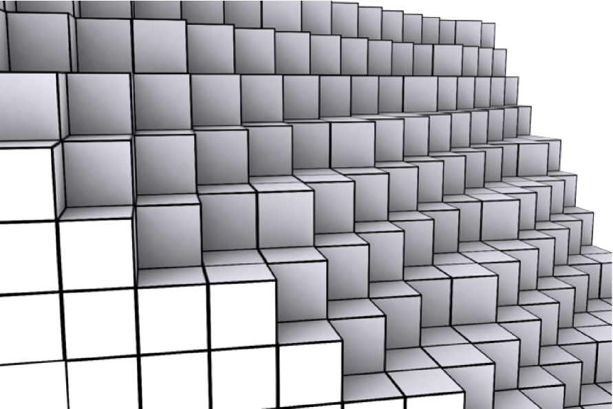
Figure 3: A non-hypergeometric quadrangulation - which points are of positive, zero and negative curvature? (graphics: courtesy of Mick West)

In the Gaussian case, one has an analogous modification.

Problem G^′. Classify all covers $f:\mathbb{P}^{1}\rightarrow\mathbb{P}^{1}$ such that $f$ has ramification index 2 or 1 at each fiber above $0\in\mathbb{P}^{1}$, ramification index 4, 2 or 1 at each fiber above $1\in\mathbb{P}^{1}$ and has $k_{i}\geq 0$ points of ramification index $i$ above $\infty\in\mathbb{P}^{1}$ for $i=1,2,3,\dots$.

Suppose $f$ is of degree $d$. Let $m_{i}$ be the number of points above $0$ of ramification index $i$ for $i=1,2$. Similarly, let $n_{i}$ be the number of points above $1$ of ramification index $i$ for $i\in\{1,2,4\}$. Thus, $m_{1}+2m_{2}=n_{1}+2n_{2}+4n_{4}=\sum_{i=1}^{\infty}ik_{i}=d$.The Riemann-Hurwitz formula yields

$$2=-d+(m_{1}+m_{2})+(n_{1}+n_{2}+n_{4})+\sum_{i=1}^{\infty}k_{i}.$$ (4.7)

Therefore

$$2=-\frac{d}{4}+\frac{m_{1}}{2}+\frac{3n_{1}+2n_{2}}{4}+\sum_{i=1}^{\infty}k_{i},$$

and setting $d=\sum_{i=1}^{\infty}ik_{i}$ yields

$$\sum_{i=1}^{\infty}(4-i)k_{i}=8-2m_{1}-3n_{1}-2n_{2}.$$ (4.8)

The case $m_{1}=n_{1}=n_{2}=0$ was considered in Problem G. Assuming that at least one of $m_{1}$, $n_{1}$ and $n_{2}$ is non-zero, we get the table in Appendix 3.

Figure 4: A hypergeometric sphere triangulation

5 Thurston’s work on sphere triangulations

We must stress that the lists of the previous section are purely hypothetical. Numerology exhibits potentialities but doesn’t say anything about their realizations. Attacking this problem in a straightforward manner requires studying monodromy presentations, which is a time and space consuming combinatorial problem that one may hope to attack by a computer. In contrast with this, one of the results stated in Thurston’s 1987 preprint is the following theorem

Theorem (Thurston, [42]) (Polyhedra are lattice points) There is a lattice ${\cal L}$ in complex Lorenz space $\mathbf{C}^{(1,9)}$ and a group $\Gamma_{DM}$ of automorphisms, such that sphere triangulations of non-negative combinatorial curvature are elements of ${\cal L}_{+}/\Gamma_{DM}$, where ${\cal L}_{+}$ is the set of lattice points of positive square-norm. The square norm of a lattice point is the number of triangles in the triangulation. The projective action of $\Gamma_{DM}$ on complex projective hyperbolic space $\mathbf{C}{\mathbb{H}}^{9}$ (the unit ball in $\mathbf{C}^{9}\subset\mathbf{C}{\mathbb{\mathbb{P}}}^{9}$) has quotient of finite volume.

This lattice was explicitly identified by Allcock [3]. Triangulations lying on the same line through the origin are simultaneous subdivisions of a “primitive” triangulation on the line and therefore define isometric polyhedra. Hence the projectification

$$\mathbb{P}{\cal L}_{+}/\Gamma_{DM}\subset{\cal M}_{DM}:=\mathbf{C}{\mathbb{H}}^{9}/\Gamma_{DM}$$

classifies the isometry classes (“shapes” in Thurston’s terms) of polyhedra, where ${\cal M}_{DM}$ is the ball-quotient space $\mathbf{C}{\mathbb{H}}^{9}/\Gamma_{DM}$. We shall call these “hypergeometric points” of the moduli space. Thurston also describes a very explicit method to construct these triangulations and gives the estimation $O(n^{10})$ for the number of triangulations in $HG_{Eis}([1]_{12})$ with up to $2n$ triangles.

Problem: (Isomer counting) Let $\Delta_{n}(\mu)$ be the number of triangulations in $HG(\mu)$ with $n$ triangles. Find an appropriate generating function $T_{\mu}$ for the numbers $\Delta_{n}(\mu)$.

It must be possible to complete Thurston’s results as follows:

Theorem. Let $\mu$ be an admissible curvature vector of length $\ell(\mu)=\ell$. There is a lattice ${\cal L(\mu)}$ in complex Lorenz space $\mathbf{C}^{(1,\ell-3)}$ and a group $\Gamma(\mu)$ of automorphisms, such that triangulations of type $\mu$ are elements of ${\cal L}_{+}(\mu)/\Gamma(\mu)$, where ${\cal L}_{+}(\mu)$ is the set of lattice points of positive square-norm. The projective action of $\Gamma{(\mu)}$ on complex projective hyperbolic space $\mathbf{C}{\mathbb{H}}^{\ell-3}$ (the unit ball in $\mathbf{C}^{\ell-3}\subset\mathbf{C}{\mathbb{\mathbb{P}}}^{\ell-3}$) has quotient of finite volume. The square norm of a lattice point is the number of triangles in the triangulation.

The previous theorem corresponds to the longest parameter $\mu=[1]_{12}$, and the other pairs $({\cal L(\mu)},\Gamma(\mu))$ arise as degenerations of this one. As abstract groups, $\Gamma{(\mu)}$ are braid group quotients. We denote the quotient

$$\mathbf{C}{\mathbb{H}}^{\ell-3}/\Gamma(\mu)=:\mathcal{M}_{\mu}.$$

As above, there is a dense subset of hypergeometric points inside the ball quotient space $M_{\mu}$:

$$\mathbb{P}{\cal L_{+}(\mu)}/\Gamma(\mu)\subset{\cal M}_{\mu}.$$

These points are conjecturally defined over $\overline{\mathbb{Q}}$. It is an important task to understand the structure of the “hypergeometric web” , i.e. various degenerations of triangulations in this 9-dimensional moduli space (with respect to the Galois action). Even the integral lattices themselves have not been explicitly identified in the literature. İsmail Sağlam [33], [32] proved this theorem for the cases $\mu=[2]_{6}$ and $\mu=[3]_{4}$ (and also $\mu=[1]_{12}$), using alternative and more explicit methods than Thurston’s hard-going paper. His proof gives a construction of those triangulations and also applies to Ayberk Zeytin’s theorem concerning quadrangulations presented below. In case $\mu=[3]_{4}$, the group in question is the modular group, i.e. $\Gamma([3]_{4})\simeq\mathrm{PSL}_{2}(\mathbb{Z})$ and provides the most amenable family of triangulations and polyhedra on which the Galois action should be studied. We shall give a construction of this family in the last section of the current paper.

Allcock gave in the late 1990’s a more direct construction of $\Gamma_{DM}$ as a group of automorphisms of the lattice ${\cal L}$ and imitated this construction to build a 13-dimensional ball quotient related to a lattice ${\cal L}^{A}$ which is derived from the Leech lattice [3]. His construction is conjecturally related to the Monster group in a precise way [4]. The connection we unearthed above between the hypergeometric triangulations and the quilts related to the monster (see [21], Chapter 11) reveals that there is something about the monster in the hypergeometric world. Is there a similar combinatorial interpretation of Allcock’s lattice ${\cal L}^{A}$ i.e. as a set of triangulations? If yes, most of the questions we raise here about the Deligne-Mostow’s ball quotients and related objects could be formulated for Allcock’s ball-quotient as well.

As for the quadrangulations, one has the following result

Theorem (Ayberk Zeytin [51], [45]) (Quadrangulations are lattice points) There is a lattice ${\cal L}$ in complex Lorenz space $\mathbb{C}^{(1,8)}$ and a group $\Gamma_{DM}$ of automorphisms, such that quadrangulations of non-negative combinatorial curvature are elements of ${\cal L}_{+}/\Gamma_{DM}$, where ${\cal L}_{+}$ is the set of lattice points of positive square-norm. The projective action of $\Gamma_{DM}$ on complex projective hyperbolic space $\mathbf{C}{\mathbb{H}}^{9}$ (the unit ball in $\mathbf{C}^{9}\subset\mathbf{C}{\mathbb{\mathbb{P}}}^{9}$) has quotient of finite volume. The square of the norm of a lattice point is the number of quadrangles in the triangulation.

Figure 5: A hypergeometric sphere quadrangulation

5.1 Hypergeometric functions, ball-quotients of Picard, Terada, Deligne and Mostow and the transcendence results of Wolfart and Shiga.

Multivariable hypergeometric functions arise as the uniformization maps of the moduli spaces ${\mathcal{M}}_{\mu}$.

The hypergeometric differential equation was first discovered by Euler, the term hypergeometric is even older; the name Gauss’ hypergeometric functions is also frequently used after Gauss’s contributions. Appell introduced a two-variable hypergeometric function, which was further generalized to arbitrary many variables by Lauricella. Following the works of Riemann and Schwarz in dimension one, Picard studied the finiteness and discreteness of monodromy for Appell’s hypergeometric functions. Terada extended this work to the Lauricella hypergeometric functions in the 1970’s. Deligne and Mostow’s paper on Lauricella hypergeometric functions appeared in the1980’s and gave a uniform and rigorous treatment of discreteness using algebraic geometry (see [28] for an elementary treatment). Thurston used geometric methods to reprove these discreteness results, without mentioning hypergeometric functions at all [42]. By using the numerical ball-quotient criterion (Miyaoka-Yau proportionality) Hirzebruch, Holzapfel and followers discovered some other discrete complex hyperbolic groups generated by reflections, but they all turned out to be commensurable with a lattice in Picard-Terada-Deligne-Mostow’s (PTMD) list [12]. Recently, Heckman-Couwenberg-Looijenga gave another generalization and obtained some other complex hyperbolic reflection groups [9]. However, it is not known if these lattices are commensurable with the PTMD lattices. Yoshida and collaborators gave alternative modular interpretations of hypergeometric functions and studied their properties [49].

Transcendence problems for the (multivalued) Schwarz maps have been studied by Cohen, Wohlfart, Shiga and Suzuki, their result for higher dimensions roughly reads: “if the Schwarz map value at $\tau$ is algebraic, then a certain Prym variety parametrized by $\tau$ has CM”. On the reverse direction, it is a natural wonder what the images of lattice points under the ball-quotient maps (inverse Schwarz maps) are. Is it possible to compute their precise values? We conjecture that the images of lattice points are dense, and algebraic. Finally, the Galois action is compatible with the action on the corresponding hypergeometric curves. Moreover, the Galois action must respect the structure of the “hypergeometric web”, which is formed by the degenerations in the 9-dimensional ancestral ball-quotient.

5.2 Questions.

In the light of their connections to hypergeometric functions, combinatorics and group theory, there is a well-founded hope that hypergeometric curves will render themselves to explicit calculation and unlike the case of a general dessin, we can study the Galois action on them. There are several circles of questions that appear:

By “hypergeometric triangulation or quadrangulation” (equivalently “hypergeometric dessin”) of type $\mu$, we both mean a point in ${\mathcal{L}}(\mu)$ and the sphere triangulation defined by this point. “Hypergeometric curve” (or “hypergeometric cover”) of type $\mu$ means the covering of the Riemann sphere defined by a hypergeometric triangulation of type $\mu$. A “hypergeometric point” of type $\mu$ is an element of $\mathbb{P}{\cal L_{+}(\mu)}/\Gamma(\mu)\subset{\cal M}_{\mu}$, in other words it is a shape parameter of a polyhedra. Every hypergeometric point represents a ray of hypergeometric triangulations, all obtained from a basic triangulation by simultaneous subdivision.

5.2.1 Group theory and combinatorics.

Which hypergeometric curves are modular (i.e. dominated by congruence modular curves)? Given a hypergeometric curve, find the smallest Galois cover that dominates it. Characterize the monodromy groups of hypergeometric covers. Compare these monodromy groups with nilpotent and solvable groups; are these groups non-abelian in an essential manner? Given two hypergeometric covers, find the (dessin of) smallest covering that dominates both. Find also the smallest Galois covering that dominates both. Find an appropriate generating function for the number of hypergeometric triangulations of the same type $\mu$ (isomer counting).

5.2.2 Field theory and Galois action.

Given a hypergeometric triangulation, describe the corresponding Belyi map explicitly and study the Galois action. Are the Galois action on ${\cal L_{+}(\mu)}/\Gamma(\mu)$ (defined via hypergeometric curves) and the Galois action on the hypergeometric points $\mathbb{P}{\cal L_{+}(\mu)}/\Gamma(\mu)$ compatible? Does this action respect degeneration of triangulations? Is the Galois action faithful on hypergeometric curves? (probably it isn’t).

Describe the fields of definitions of hypergeometric covers. Describe the minimal field of definitions $F_{\mu}^{d}$ of hypergeometric covers of the same type $\mu$ and degree $d$, and estimate the order of growth of $[F_{\mu}^{d}:\mathbb{Q}]$ as $d\rightarrow\infty$. Describe the minimal field of definition of all hypergeometric covers of the same type $\mu$. Characterize the minimal field of definition of all hypergeometric covers.

5.2.3 Moduli space, transcendence, rational point counting.

Show that the hypergeometric points are dense. Calculate some hypergeometric points explicitly. Is it possible to obtain a triangulation represented by a hypergeometric point ? Describe the fields of definitions of hypergeometric points. Give examples of non-hypergeometric algebraic points of ${\cal M}_{\mu}$.

The minimal number of triangles of hypergeometric triangulations represented by a hypergeometric point $p_{\cal T}$ defines a “height” function on the points $p_{\cal T}$. Describe the minimal field of definitions $K_{\mu}^{d}$ of hypergeometric points of the same type $\mu$ and height, and estimate the order of growth of $[K_{\mu}^{d}:\mathbb{Q}]$ as $d\rightarrow\infty$. Describe the minimal field of definition of all hypergeometric points of the same type $\mu$. Characterize the minimal field of definition of all hypergeometric points. Count the hypergeometric points.

5.2.4 Moonshine.

Elucidate the connections between the netballs of Norton (group theory), triangulations of non-negative curvature of Thurston (geometry), hypergeometric curves (algebraic geometry) and Allcock’s “monstrous proposal” (complex hyperbolic geometry). We invite you to inspect the quilts in [21] to realize that they are all hypergeometric.

5.2.5 Hypergeometric Grothendieck-Teichmüller Theory.

The $\overline{{\cal M}}_{DM}$ includes all families of hypergeometric triangulations as degenerations. Let us call this structure the “hypergeometric web”. Devise a hypergeometric version of the Grothendieck-Teichmüller group $\widehat{GT}$, deduced from the relations of the “hypergeometric web” instead of the greater Teichmüller tower.

5.2.6 Other lattices.

Thurston’s article includes more lattices than those classifying the hypergeometric triangulations and hypergeometric square tilings. Is there a combinatorial interpretation of these lattices, similar to triangulations or tilings? Are these lattices connected to some arithmetic curves in some other way? Do they admit a Galois action?

5.3 Hypergeometric completion of the profinite modular group.

Let $G$ be a finitely presented group and let $\widehat{G}$ be its profinite completion. Let ${\mathbb{H}}=\{H_{\alpha}\}_{\alpha\in I}$ be a system of finite index subgroups of $G$, satisfying the property:

(*) for any $i\in\mathbb{Z}_{>0}$, there are only a finite number of $\alpha$’s such that $[G:H_{\alpha}]\leq i$.

To ${\mathbb{H}}$, one may of associate a quotient $\widehat{G}_{\mathbb{H}}$ of $\widehat{G}$ as follows: Let $\overline{\mathbb{H}}:=\{\overline{H}_{\alpha}\}_{\alpha\in I}$, where $\overline{H}_{\alpha}:=\bigcap_{g\in G}gH_{\alpha}g^{-1}$ is the normal core of $H_{\alpha}$. Then $\overline{\mathbb{H}}$ also satisfies the property (*), and the normal subgroups

$$H(i):=\bigcap_{[G:H_{\alpha}]\leq i}H_{\alpha}$$

are of finite index in $G$ as well. Then $G\rhd H(1)\rhd H(2)\rhd\dots$ is a chain of normal subgroups of $G$. Put $\widehat{G}_{\mathbb{H}}:=\lim_{\leftarrow}G/H(i)$. One may call $\widehat{G}_{\mathbb{H}}$: “the completion of $G$ with respect to the system ${\mathcal{H}}$”. Any system ${\mathbb{H}}$ can be enriched by the set of all co-nilpotent (or co-pro-$\ell$, or co-solvabe.) normal subgroups of all elements in ${\mathbb{H}}$, yielding a greater system and an induced “enriched” completion.

If we take $G=\mathrm{PSL}(2,\mathbb{Z})$ and ${\cal H}=HG(\mu)$, then the above procedures yield completions (“enriched” if we wish) $\widehat{\mathrm{PSL}}^{\mu}(2,\mathbb{Z})$. This is a somewhat artificial construction, but it seems that this is the only algebraic object at our immediate disposal, which is derived from hypergeometry and on which we can study the Galois representation (and not merely a Galois action). Questions: Is $\widehat{\mathrm{PSL}}^{\mu}(2,\mathbb{Z})$ metamotivic? meaning: is it essentially “larger” from almost nilpotent completions? What is the kernel of the corresponding Galois representation? Can we get an analogue of the Grothendieck-Teichmüller group by considering the total structure of the hypergeometric web?

6 Case study: the simplest families of triangulations and quadrangulations

Here we give an overview of some results from the second named author’s thesis [33] to describe the family of triangulations $HG_{Eis}([3]_{4})$ and the family of quadrangulations $HG_{Gauss}([2]_{4})$. The set $HG_{Eis}([3]_{4})$ is the set of triangulations with 4 singular vertices (vertices of non-zero combinatorial curvature) such that each of these vertices is incident to 3 triangles. Similarly, $HG_{Gauss}([2]_{4})$ is the set of quadrangulations with 4 singular vertices such that each singular vertex is incident to 2 quadrangles.

We need to introduce some terminology from the theory of cone metrics on 2-dimensional surfaces.

6.1 Cone Metrics on Surfaces

Our reference in this section is [43] and [44]. A triangulated surface is roughly a surface with an Euclidean triangulation on it. Here is the formal definition.

Definition 6.1.

A triangulated surface is a surface $S$ together with a set of pairs $\mathbf{T}=\{(T_{\alpha},f_{\alpha})\}_{\alpha\in A}$ where each $T_{\alpha}$ is a compact subset of $S$ and each $f_{\alpha}:T_{\alpha}\rightarrow\mathbb{R}^{2}$ a diffeomorphism with a non-degenerate euclidean triangle such that

• $T_{\alpha}$’s cover $S$.

• If $\alpha\neq\beta$ then intersection of $T_{\alpha}$ and $T_{\beta}$ is either empty or edge or a vertex.

• If $T_{\alpha}\cap T_{\beta}$ is not empty then there is an element $g_{\alpha\beta}$ $\in E(2)$ (the group of isometries Euclidean plane) such that $f_{\alpha}=g_{\alpha\beta}f_{\beta}$.

Definition 6.2.

A cone metric on a triangulated surface is a metric obtained by using given triangulation.

A surface with a cone metric will be called flat surface. It is clear that for each point $p$ on a flat surface $S$ there is a notion of angle, $\theta_{p}$. The value $\kappa_{p}=2\pi-\theta_{p}$ is called the curvature at $p$. With this preparation we may present the Gauss-Bonnet Theorem and Hopf-Rinow Theorem for flat surfaces:

Theorem 6.3.

(Gauss-Bonnet) Denote by $\chi(S)$ the Euler charateristic of $S$. For any compact flat surface $S$ without boundary we have

$$\sum_{p\in S}(2\pi-\theta_{p})=\chi(S).$$

This formula is easily established by summing angles at singular vertices and counting number of triangles used.

Theorem 6.4.

(Hopf-Rinow) Let $S$ be a complete, connected, flat surface. Then any two points in $S$ can be joined by a shortest geodesic in $S$.

How can we obtain cone metrics on sphere? To be more precise, assume that we are given positive numbers $\theta_{1},\theta_{2},\theta_{3}$ so that

$$\theta_{1}+\theta_{2}+\theta_{3}=2\pi.$$ (6.9)

Can we find a cone metric with 3 singular points such that cone angles at these points are $\theta_{1},\theta_{2}$ and $\theta_{3}$? Answer for this question is affirmative, see Figure  6.

Figure 6: Constructing a cone metric with 3 singular points

In Figure  6 lengths of $l_{1}$ and $l_{1}^{\prime}$ are equal. Also lengths of $l_{2}$ and $l_{2}^{\prime}$ are equal. If we glue $l_{1}$ with $l_{1}^{\prime}$ and $l_{2}$ with $l_{2}^{\prime}$ , we get a cone metric on sphere with desired properties. Indeed, this is the only cone metric with above property up to homothety and orientation preserving isometry.

At this point, it is natural to ask whether every cone metric on sphere can be obtained from a polygon in Euclidean plane by identifying some of its edges appropriately. This is not possible in general. However, if all curvatures at singular points are positive, the answer is affirmative and is given by Alexandrov Unfolding Process.

6.1.1 Alexandrov Unfolding Process.

Let $\mu$ be a cone metric on sphere with $n$ ($n>2$) singular points of positive curvature. Call these singular points $v_{1},v_{2},\dots,v_{n}$. Let $s_{i}$ ($2\leq i\leq n$) be a length minimizing geodesic joining $v_{1}$ to $v_{i}$. These geodesics exists by Hopf-Rinow Theorem. It is well known that $s_{i}$ and $s_{j}$ intersect at only $v_{1}$ when $i\neq j$. If we cut sphere along $s_{i}$’s, then we can unfold it to the plane without overlapping as a polygon with $2n-2$ vertices. Resulting polygon $P$ has $n-1$ vertices coming from $v_{1}$ and $n-1$ vertices corresponding to $v_{i}$’s ($i>1$). If we glue edeges of this polygon appropriately we get a cone metric on sphere with $n$ singular points. Indeed, this metric, after some normalization, is nothing else than $\mu$.

This process, Alexandrov Unfolding, briefly says that any cone metric of the positive curvature on sphere can be obtained from a special type of polygon in the plane.

6.2 Triangulations

Up to now, we have talked about cone metrics. Now we start to investigate triangulations of sphere. We consider, following [42], a triangulation as a cone metric by assuming that each triangle in triangulation is Euclidean equilateral triangle of edge length 1. We say that two triangulations are equivalent if corresponding metrics are isometric by an orientation preserving isometry sending edges, vertices and triangles to edges, vertices and triangles, respectively.

How can we construct sphere triangulations? We don’t have any means of constructing and classifying them in a systematic manner, other then drawing them by hand. So let us ask a simpler question: How can we obtain elements in $HG_{Eis}([4]_{3})$?

Figure 7: Obtaining an element of $HG_{Eis}([4]_{3})$ from a lattice point.

Let $\mathbf{Eis}$ be the ring of Eisenstein integers. Observe that $\mathbf{Eis}$ gives a triangulation of the plane. We will obtain desired triangulations from this triangulation. Consider the polygon in Figure  7 with the following properties:

• vertices of the polygon are in $\mathbf{Eis}$,

• lengths of $l_{1}$ and $l_{1}^{\prime}$ are equal,

• lengths of $l_{2}$ and $l_{2}^{\prime}$ are equal,

• angles at $\alpha$ and origin are $\frac{2\pi}{3}$,

• angles at the other two vertices are $\frac{\pi}{3}$.

If we glue $l_{1}$ with $l_{1}^{\prime}$ and $l_{2}$ with $l_{2}^{\prime}$ we get a triangulation of sphere. Moreover the vertices corresponding to $0$ and $\alpha$ are incident to two triangles. Also the other two vertices form a single vertex of the triangulation which is incident to two triangles. Therefore we obtain an element in $HG_{Eis}([4]_{3})$.

It is natural to ask whether all elements in $HG_{Eis}([4]_{3})$ can be obtained in this manner. The answer is affirmative. Start with a triangulation of desired type and unfold it to the plane accordingly by Alexandrov Unfolding Process. The polygon you get has the properties described before. Glue it as before to get the triangulation back.

It is also natural to ask whether two different polygons satisfying above properties give rise to different triangulations. In this case answer is not affirmative. To see this, first observe that any such polygon is uniquely determined by it’s vertex $\alpha$. Let $\delta=e^{\frac{2\pi\sqrt{-1}}{6}}$. If we change $\alpha$ with $\delta\alpha$, original polygon will be rotated in counter-clockwise direction by an angle of $\frac{2\pi}{6}$ around the origin. Therefore triangulation will not be changed. Hence we have a map

$$\mathbf{Eis}/\langle\delta\rangle\rightarrow HG_{Eis}([4]_{3})$$ (6.10)

and indeed, this map is also injective.

Observe that area of the polygon is proportional to the square-norm $\alpha\overline{\alpha}$, hence, square-norm of a lattice point gives number of triangles in the triangulation. This case, $HG_{Eis}([4]_{3})$, is also explained in [42].

We summarize the results of this section in the following theorem.

Theorem 6.5.

There is a bijection

$$\mathbf{Eis}/\langle\delta\rangle\equiv HG_{Eis}([4]_{3})$$ (6.11)

such that square-norm of a lattice point gives number of triangles in corresponding triangulation.

6.3 Shapes of Tetrahedra

Let $C(\pi,\pi,\pi,\pi)$ be the set of cone metrics on sphere with four singular points of cone angle $\pi$, up to homotety and orientation preserving isometry. The aim of this section is to describe this set.

Consider the following complex vector space

$$H=\{(z_{1},z_{2}):z_{1},z_{2}\in\mathbb{C}\},$$ (6.12)

with the Hermitian form

$$\langle(z_{1},z_{2}),(w_{1},w_{2})\rangle=\frac{\sqrt{-1}}{4}\{z_{1}\bar{w_{2}}-z_{2}\bar{w_{1}}\}.$$ (6.13)

If we regard an element $(z_{1},z_{2})$ as triangle in complex plane with vertices $0,z_{1},z_{2}$, the square-norm of $(z_{1},z_{2})$

$$\frac{\sqrt{-1}}{4}\{z_{1}\bar{z_{2}}-z_{2}\bar{z_{1}}\}.$$

gives signed area of the triangle, see Figure 8.

Figure 8: Cone Metric from an element in $H^{+}$

Since there are both triangles of positive area and triangles of negative area, signature of this area Hermitian form is $(1,1)$. Let

$$H^{+}=\{z\in H:\langle z,z\rangle>0\}.$$ (6.14)

be the positive part of $H$ with respect to area Hermitian form. $H^{+}$ consists of positively oriented triangles. There is a nice way to obtain cone metrics from these triangles. Consider the triangle in Figure 8 again. Glue the line segment $a$ with $a^{\prime}$ and $b$ with $b^{\prime}$. By this way we obtain a cone metric on sphere. It is clear that angles at the vertices corresponding to $\frac{z_{1}}{2},\frac{z_{2}}{2},\frac{z_{1}+z_{2}}{2}$ are $\pi$. Also observe that the vertices $0,z_{1},z_{2}$ come together to form a vertex having angle $\pi$. Therefore we get an element in $C(\pi,\pi,\pi,\pi)$.

Figure 9: First Cutting Operation

Can every element in $C(\pi,\pi,\pi,\pi)$ be obtained from an element in $H^{+}$ by using the process above? Indeed, by Alexandrov Unfolding Process, we can cut-open an element in $C(\pi,\pi,\pi,\pi)$ to a polygon, actually a triangle, in $H^{+}$. We can glue edges of this triangle to get the cone metric back. Therefore we have a surjective map

$$H^{+}\rightarrow C(\pi,\pi,\pi,\pi).$$ (6.15)

This map is far away from being injective. Let $\alpha\in\mathbb{C}$ be a complex number and $(z_{1},z_{2})\in H^{+}$. The triangle

$$\alpha(z_{1},z_{2})=(\alpha z_{1},\alpha z_{2})$$

is obtained by rotating (around origin) and rescaling the triangle $(z_{1},z_{2})$. Therefore triangles $(z_{1},z_{2})$ and $\alpha(z_{1},z_{2})$ give rise to the same element in $C(\pi,\pi,\pi,\pi)$. Hence we have a map

$$\mathbb{P}H^{+}=\mathbb{H}=\mathbb{H}_{\mathbb{C}}^{1}\rightarrow C(\pi,\pi,\pi,\pi).$$ (6.16)

where $\mathbb{P}H^{+}$ is complex projectification of $H^{+}$ which is same as one dimensional complex hyperbolic space and 2 dimensional real hyperbolic space.

This map is not injective neither. Consider Figure 9. Given the triangle $(z_{1},z_{2})$ in $H^{+}$, we cut it through the line segment $[0,\frac{z_{1}+z_{2}}{2}]$ and glue edges $b$ with $b^{\prime}$ by a rotation of angle $\pi$ around $\frac{z_{1}+z_{2}}{2}$ to get the triangle $(z_{1},z_{1}+z_{2})$. Observe that the following elements gives the same cone metric:

$$\begin{pmatrix}z_{1}\\ z_{2}\end{pmatrix}\,\mbox{ and }\,\begin{pmatrix}1&0\\ 1&1\end{pmatrix}\begin{pmatrix}z_{1}\\ z_{2}\end{pmatrix}=\begin{pmatrix}z_{1}\\ z_{1}+z_{2}\end{pmatrix}$$

Figure 10: Second Cutting Operation

Now consider Figure 10. Cut the triangle $(z_{1},z_{2})$ from the line segment $[z_{2},\frac{z_{1}}{2}]$ and glue $a$ with $a^{\prime}$ by a rotation of angle $\pi$ around $\frac{z_{1}}{2}$. You will get the triangle $(z_{1}-z_{2},z_{2})$ as in Figure 10.

Observe that the following elements gives the same cone metric.

$$\begin{pmatrix}z_{1}\\ z_{2}\end{pmatrix}\,\mbox{ and }\,\begin{pmatrix}1&-1\\ 0&1\end{pmatrix}\begin{pmatrix}z_{1}\\ z_{2}\end{pmatrix}=\begin{pmatrix}z_{1}-z_{2}\\ z_{2}\end{pmatrix}$$

The group generated by the matrices

$$\begin{pmatrix}1&0\\ 1&1\end{pmatrix},\begin{pmatrix}1&-1\\ 0&1\end{pmatrix}$$ (6.17)

in $\mathrm{PSL}(2,\mathbb{R})$ is the modular group $\mathrm{PSL}(2,\mathbb{Z})$. Thus there is a well-defined map

$$\mathbb{P}H^{+}/\mathrm{PSL}(2,\mathbb{Z})\rightarrow C(\pi,\pi,\pi,\pi)$$ (6.18)

We summarize results obtained in this section as follows:

Theorem 6.6.

There is a map

$$\mathbb{P}H^{+}/\mathrm{PSL}(2,\mathbb{Z})\rightarrow C(\pi,\pi,\pi,\pi)$$ (6.19)

which is both injective and surjective.

This bijection is not just a set theoretic bijection: one can naturally give, in some sense, complex structures to both $\mathbb{P}H^{+}/\mathrm{PSL}(2,\mathbb{Z})$ and $C(\pi,\pi,\pi,\pi)$. The bijection above respects these structures. Also observe that above theorem means that $C(\pi,\pi,\pi,\pi)$ is nothing else than the modular orbifold.

6.4 Back to triangulations

Set $\mathbb{E}^{+}=\mathbb{E}\cap H$, where

$$\mathbb{E}=2\mathbf{Eis}\bigoplus 2\mathbf{Eis}=\{z=(2z_{1},2z_{2}):z_{i}\in\mathbf{Eis}\}\subset H.$$

Our next objective is to derive triangulations of type $[3]_{4}$ from $\mathbb{E}^{+}$. Observe that the elements in $\mathbb{E}^{+}$ can be thought as positively oriented triangles whose vertices and midpoints of the edges are in $\mathbf{Eis}$. See Figure 11.

Figure 11: Triangulations from Eisenstein Lattice

There is a well-defined map

$$\mathbb{E}^{+}\rightarrow HG_{Eis}([3]_{4}),$$ (6.20)

given as follows. Take an element $(2z_{1},2z_{2})$ as in Figure 11. Glue the segment $[0,z_{1}]$ with $[z_{1},2z_{1}]$ as we did before. Do the same for the segments $[2z_{1},z_{1}+z_{2}]$, $[z_{1}+z_{2},2z_{2}]$ and $[2z_{2},z_{2}]$, $[0,z_{2}]$. By this way, we get a triangulation of the sphere. Observe that the vertices incident to $z_{1},z_{2},z_{1}+z_{2}$ are incident to 3 triangles. The vertices $0,2z_{1},2z_{2}$ come together to form just one vertex of the triangulation which is also incident to 3 triangles. Therefore we obtain an element in $HG_{Eis}([3]_{4})$.

This map is surjective by Alexandrov Unfolding Process, one can cut-open a triangulation to obtain an element in $\mathbb{E}^{+}$ and glue this element appropriately to get the initial triangulation back.

This map is not injective. First of all, if $(2z_{1},2z_{2})\in\mathbb{E}^{+}$ is a triangle, then multiplication by $\delta=e^{\frac{2\pi\sqrt{-1}}{6}}$ transforms this triangle to $(2\delta z_{1},2\delta z_{2})\in\mathbb{E}^{+}$ which is a triangle obtained by rotating the former triangle by an angle of $\frac{2\pi}{6}$ around origin. Therefore it does not change triangulation. Also cutting and gluing operations defined in the pervious section respect triangulations. Hence we have a map

$$\mathbb{E}^{+}/\langle\delta\rangle\times\mathrm{SL}(2,\mathbb{Z})\rightarrow HG_{Eis}([3]_{4}).$$ (6.21)

This map is both injective and surjective. The area Hermitian form

$$\langle(z_{1},z_{2}),(w_{1},w_{2})\rangle=\frac{\imath}{4}\{z_{1}\bar{w_{2}}-z_{2}\bar{w_{1}}\}.$$ (6.22)

defined in the previous section gives the area of the triangle considered. Therefore if we restrict our attention to $\mathbb{E}^{+}$, it gives us number of triangles in corresponding triangulation. Next theorem summarizes the results obtained in this section. See also [32], [33], [42].

Theorem 6.7.

There is a bijection

$$\mathbb{E}^{+}/\langle\delta\rangle\times\mathrm{SL}(2,\mathbb{Z})\equiv HG_{Eis}([3]_{4}),$$ (6.23)

such that the square-norm of each element gives number of triangles in the triangulation.

6.5 Shapes of quadrangulations

Set $\mathbb{G}^{+}=\mathbb{G}\cap H$, where $\mathbb{G}$ is given by

$$\mathbb{G}=2\mathbb{Z}[\sqrt{-1}]\bigoplus 2\mathbb{Z}[\sqrt{-1}]=\{z=(2z_{1},2z_{2}):z_{1},z_{2}\in\mathbb{Z}[\sqrt{-1}]\}\subset H$$

We will obtain quadrangulations of type $[2]_{4}$ from $\mathbb{G}^{+}$. We consider quadrangulations as cone metrics by assuming that each quadrangle is unit square. Observe that element in $\mathbb{G}^{+}$ can be regarded as triangles in complex plane whose vertices and midpoints of the edges are in the ring of Gaussian integers; $\mathbb{Z}[\sqrt{-1}]$. See Figure 12.

Figure 12: Quadrangulations from Gaussian Lattice

Gluing process explained before provides us a map

$$\mathbb{G}^{+}\rightarrow HG_{Gauss}([2]_{4}).$$ (6.24)

This map is surjective by Alexandrov Unfolding Process, but it is not injective. Multiplication of a lattice element by $\sqrt{-1}$ just rotates the triangle by an angle of $\frac{\pi}{2}$ around origin; thus it respects quadrangulation. Also cutting and gluing operations defined before respect quadrangulation. We have a map

$$\mathbb{G}^{+}/\langle\sqrt{-1}\rangle\times\mathrm{SL}(2,\mathbb{Z})\rightarrow HG_{Gauss}([2])_{4}.$$ (6.25)

which is both injective and surjective.

Observe that area Hermitian form give the number of quadrangles in corresponding quadrangulation. Following theorem summarizes the results obtained in this section.

Theorem 6.8.

There is a bijection

$$\mathbb{G}^{+}/\langle\sqrt{-1}\rangle\times\mathrm{SL}(2,\mathbb{Z})\equiv HG_{Gauss}([2]_{4})$$ (6.26)

such that square-norm of each element gives number of quadrangles in the quadrangulation.

7 Beyond Hypergeometric

It must be possible to extend the classification of results of triangulations of non-negative curvature to more general triangulations (same for the quadrangulations). To achieve this, we need the right conditions to control the curvature. Suggestions: “just one point of negative curvature above infinity”, or “just one point of negative curvature above infinity, whose curvature is bounded below by $\kappa$ ”, or “just one point of fixed curvature $\kappa$ above infinity” (in each case, the points of non-negative curvature are arbitrary). We may also allow for a fixed number of points with controlled negative curvature. These relaxed conditions may bring in non-discrete groups into the picture, the signatures of the Hermitian forms will change, complex hyperbolic structure will decay, and there is a possibility that the parameter spaces will brake up into disconnected components. On the other hand, the relaxed conditions may lead to the discovery of other arithmetic and non-arithmetic discrete groups acting on some symmetric or non-symmetric spaces, e.g. “complex deSitter spaces”.

If we further relax the control of the points of negative curvature by simply requiring that it be bounded globally from below, then things will totally go out of control. Indeed it is easy to illustrate how wild things may become in terms of quadrangulations. Consider a big cube as in Figure 5, with $6n^{2}$ quadrangles. Its surface is a hypergeometric sphere quadrangulation (there are 8 points of positive curvature). Now imagine that this cube is made of $n^{3}$ smaller cubes. Imagine that you are a sculpture. Then by removing smaller cubes you may carve out any three-dimensional figure with galleries inside, and the curvature will remain bounded below by $-\pi/2-$ -which is already the greatest negative value that the curvature may attain in this case. In fact you may decide to glue little cubes to form self-overlaps of the 3-d figure.

It is much harder to describe the situation as the curvature goes deeper, since the shapes become non-embeddable locally in this case. So, it seems that abolishing all restrictions on the curvature (including the condition of being bounded from below) do not lead to a well-posed problem, neither.

$\blacktriangleright$It might be appropriate to conclude this text with an apology: The term “hypergeometric curve” is used in the literature to refer to some families of cyclic branched coverings of the projective line. Here this term refers to certain rigid (arithmetic) curves, which can be described by some special dessins (equivalently by triangulations, origamis, quilts, etc). Since this terminology seems to unify the rich vocabulary surrounding the hypergeometric phenomena, we could not resist the temptation to call these curves hypergeometric.

Acknowledgements. We are thankful to Athanase Papadopoulos for inviting us to publish in this volume. Both authors were funded by the grant TUBITAK-110T690. The first named is author was funded by a Galatasaray University Research Grant and the grant TUBITAK-114R073.

APPENDIX 1

dim	$k_{1}$	$k_{2}$	$k_{3}$	$k_{4}$	$k_{5}$	​deg​	​​Compct?​​	​Number​	​Pure?​	​ar?​
9	0	0	0	0	12	2	N	10	I	AR
8	0	0	0	1	10	2	N	11	I	AR
7	0	0	1	0	9	2	N	12	I	AR
7	0	0	0	2	8	2	N	13	I	AR
6	0	1	0	0	8	2	N	14	I	AR
6	0	0	1	1	7	2	N	15	I	AR
5	1	0	0	0	7	2	N	16	I	AR
6	0	0	0	3	6	2	N	17	I	AR
5	0	1	0	1	6	2	N	18	I	AR
5	0	0	2	0	6	2	N	19	I	AR
5	0	0	1	2	5	2	N	20	I	AR
4	1	0	0	1	5	2	N	22	I	AR
4	0	1	1	0	5	2	N	23	I	AR
5	0	0	0	4	4	2	N	24	I	AR
4	0	0	2	1	4	2	N	25	I	AR
3	1	0	1	0	4	2	N	26	I	AR
3	0	2	0	0	4	2	N	27	I	AR
4	0	0	1	3	3	2	N	28	I	AR
3	1	0	0	2	3	2	N	29	I	AR
3	0	1	1	1	3	2	N	30	I	AR
3	0	0	3	0	3	2	N	31	I	AR
3	0	0	0	6	0	2	N	1	P	AR
2	0	1	0	4	0	2	N	2	P	AR
2	1	1	0	0	3	2	N	32	I	AR
4	0	0	0	5	2	2	N	33	I	AR
4	0	2	0	3	2	2	N	34	I	AR
3	0	0	2	2	2	2	N	35	I	AR
2	1	0	1	1	2	2	N	36	I	AR
2	0	2	0	1	2	2	N	37	I	AR
2	1	0	2	0	2	2	N	38	I	AR
3	0	0	1	4	1	2	N	39	P	AR
2	1	0	0	3	1	2	N	40	P	AR
2	0	1	1	2	1	2	N	41	P	AR
2	0	0	3	1	1	2	N	42	P	AR
2	0	0	2	3	0	2	N	43	P	AR
1	1	0	1	2	0	-	N	-		AR
1	1	0	2	0	1	-	N	-		AR
1	1	1	0	1	1	-	N	-		AR
1	0	1	2	1	0	-	N	-		AR
1	0	2	0	2	0	-	N	-		AR
1	0	2	1	0	1	-	N	-		AR
1	0	0	4	0	0	-	N	-		AR
0	1	1	1	0	0	-	self	-
0	2	0	0	0	1	-	-	-
0	2	0	0	1	0	-	-	-
0	0	3	0	0	0	-	self	-

APPENDIX 2

dim	$m_{1}$	$n_{1}$	$k_{1}$	$k_{2}$	$k_{3}$	$k_{4}$	$k_{5}$
*6	1	0	0	0	0	0	9
*5	1	0	0	0	0	1	7
*4	1	0	0	0	1	0	6
*4	1	0	0	0	0	2	5
*3	1	0	0	1	0	0	5
*3	1	0	0	0	1	1	4
*2	1	0	1	0	0	0	4
*3	1	0	0	0	0	3	3
*2	1	0	0	0	2	0	3
*2	1	0	0	1	0	1	3
*2	1	0	0	0	1	2	2
1	1	0	0	1	1	0	2
1	1	0	1	0	0	1	2
*2	1	0	0	0	0	4	1
1	1	0	0	1	0	2	1
0	1	0	0	2	0	0	1
0	1	0	1	0	1	0	1
1	1	0	0	0	1	3	0
0	1	0	1	0	0	2	0
0	1	0	0	1	1	1	0
-1	1	0	1	1	0	0	0
*3	2	0	0	0	0	0	6
*2	2	0	0	0	0	1	4
1	2	0	0	0	1	0	3
1	2	0	0	0	0	2	2
0	2	0	0	1	0	0	2
-1	2	0	1	0	0	0	1
0	2	0	0	1	1	0	1
0	2	0	0	0	0	3	0
-1	2	0	0	0	2	0	0
0	3	0	0	0	0	0	3
-1	3	0	0	0	0	1	1
-2	3	0	0	0	1	0	0

dim	$m_{1}$	$n_{1}$	$k_{1}$	$k_{2}$	$k_{3}$	$k_{4}$	$k_{5}$
*5	0	1	0	0	0	0	8
*4	0	1	0	0	0	1	6
*3	0	1	0	0	1	0	5
*3	0	1	0	0	0	2	4
*2	0	1	0	1	0	0	4
*2	0	1	0	0	1	1	3
1	0	1	1	0	0	0	3
*2	0	1	0	0	0	3	2
1	0	1	0	0	2	0	2
1	0	1	0	1	0	1	2
1	0	1	0	0	1	2	1
0	0	1	0	1	1	0	1
0	0	1	1	0	0	1	1
1	0	1	0	0	0	4	0
0	0	1	0	1	0	2	0
-1	0	1	0	2	0	0	0
-1	0	1	1	0	1	0	0
1	0	2	0	0	0	0	4
1	0	2	0	0	1	1	2
0	0	2	1	0	1	0	1
-1	0	2	0	0	0	2	0
-2	0	2	0	1	0	0	0
-3	0	3	0	0	0	0	0
*2	1	1	0	0	0	0	5
1	1	1	0	0	0	1	3
0	1	1	0	0	1	0	2
-1	1	1	0	1	0	0	1
-2	1	1	1	0	0	0	0
-1	2	1	0	0	0	0	2
-2	2	1	0	0	0	1	0
-2	1	2	0	0	0	0	1
-3	4	0	0	0	0	0	0

APPENDIX 3

($m_{1}$, $n_{1}$, $n_{2}$)=(1,0,0) or (0,0,1)	dim $k_{1}$ $k_{2}$ $k_{3}$ 3 0 0 6 2 0 1 4 2 1 0 3 1 0 2 2 0 1 1 1 0 0 3 0 -1 2 0 0
($m_{1}$, $n_{1}$, $n_{2}$)=(0,1,0)	dim $k_{1}$ $k_{2}$ $k_{3}$ 2 0 0 5 1 0 1 3 0 1 0 2 0 0 2 1 -1 1 1 0
($m_{1}$, $n_{1}$, $n_{2}$)=(2,0,0), (0,0,2) or (1,0,1)	dim $k_{1}$ $k_{2}$ $k_{3}$ 1 0 0 4 0 0 1 2 -1 1 0 1 -1 0 2 0 0 0 0 3 -1 0 1 1 -2 1 0 0
($m_{1}$, $n_{1}$, $n_{2}$)=(1,1,0), (0,1,1)	dim $k_{1}$ $k_{2}$ $k_{3}$ 0 0 0 3 -1 0 1 1 -2 1 0 0
($m_{1}$, $n_{1}$, $n_{2}$)=(0,2,0)	dim $k_{1}$ $k_{2}$ $k_{3}$ -1 0 0 2 -2 0 1 0
($m_{1}$, $n_{1}$, $n_{2}$)=(2,1,0) or (0,1,2)	dim $k_{1}$ $k_{2}$ $k_{3}$ -2 0 0 1
($m_{1}$, $n_{1}$, $n_{2}$)=(1,2,0), (0,2,1), (4,0,0), (0,0,4)	dim $k_{1}$ $k_{2}$ $k_{3}$ -3 0 0 0

References

- [1]
- [2] N.M. Adrainov, N. Y. Amburg and V. A. Dremov, et al, Catalogue of dessins d’enfants with edges. Preprint, 2007; arXiv:0710.2658v1 [math.AG] .
- [3] D. Allcock, New complex- and quaternionic- hyperbolic reflection groups. Duke Math. J. 103 (2000), 303–333.
- [4] D. Allcock, A Monstrous proposal. Preprint, 2006; arXiv:math/0606043v2 [math.GR].
- [5] M. Atiyah and P. Sutcliffe, Polyhedra in physics, chemistry and geometry. Preprint, 2003; arXiv:math-ph/0303071v1
- [6] J. Bétréma and A. Zvonkin, Plane trees and Shabat polynomials. Discrete Math. 153 (1996), 47–58.
- [7] I. I. Bouw and M. Möller, Teichmüller curves, triangle groups, and Lyapunov exponents. Preprint, 2006; arXiv:math/0511738v2 [math.AG].
- [8] R. Boston and N. Jones, Arboreal Galois representations. Geom. Dedicata 124 (2007), 27–35 .
- [9] W. Couweberg, G. Heckman and E. Looijenga, Geometric structures on the complement of a projective arrangement. Publ. Math. IHES 101, 69–161.
- [10] P. Deligne, Le groupe fondamental de la droite projective moins trois points. In Galois groups over , MSRI Publ. 1, Springer 1989, 79–297.
- [11] P. Deligne and A. Goncharov, Groupes fondamentaux motiviques de Tate mixte. Ann. Sci. École Norm. Sup. (4) 38 (2005), 1–56.
- [12] P. Deligne and G. Mostow, Commensurabilities among lattices in . Annals of Mathematics Studies 132, Princeton University Press, Princeton, NJ, 1993.
- [13] H. Furusho, Geometric and arithmetic subgroups of the Grothendieck-Teichmüller group. Math. Res. Lett. 10 (2003), 97–108.
- [14] E. W. Godly and R. Taylor, Nomenclature and terminology of fullerenes: a preliminary survey. Pure and Applied Chemistry, 69, Blackwell Scientific, 1996.
- [15] A. Grothendieck, Revêtements étales et groupe fondamental. Lecture Notes in Math., 224, Springer-Verlag, Berlin 1971.
- [16] A. Grothendieck, La longue marche in à travers la théorie de Galois. University of Montpellier preprint series, 1996, edited by J. Malgoire.
- [17] A. Grothendieck, Esquisse d’un program. In Geometric Galois actions 1. L. Schneps et al. (Eds.) Cambridge University Press, LMS Lect. Note Ser. 242, 1997, 5-48 .
- [18] R. Hain and M. Matsumoto, Weighted completion of Galois groups and Galois actions on fundamental group of . Comp. Math. 139 (2003), 119–167.
- [19] W. J. Harvey, Teichmüller spaces, triangle groups and Grothendieck dessins. In Handbook of Teichmüller Theory. (A. Papadopoulos, ed.), Volume \@slowromancapi@, EMS Publishing House, Zurich 2007, 249-292.
- [20] F. Herrlich and G. Scmithhüsen, A comb of origami curves in the moduli space with three dimensional closure. Geom. Dedicata, to appear;: arXiv:math/0703205v1[math.AG].
- [21] T. Hsu, Quilts: Central Extansions, Braid Actions and Finite Groups. LNM 1731, Springer-Verlag, Berlin 2000.
- [22] M. Kato, On uniformizations of orbifolds. In Homotopy theory and related topics, Advanced Studies in Pure and Applied Mathematics 9, Elsevier Science, Amstardam, Newyork, 1987,149-172.
- [23] M. Kisin, What is a Galois representation? Notices AMS 54 (2007), 718–719 .
- [24] R. S. Kulkarni, An arithmetic-geometric method in the study of the subgroups of the modular group. Amer. J. Math. 113 (1991), 1053–1133.
- [25] S. K. Lando and A. K. Zvonkin, Graphs on surfaces and applications. Encylopedia of Math.141 , Spriger, 2004.
- [26] P. Lochak, Fragments of nonlinear Grothendieck-Teichmüller theory. Woods Hole math. , Ser. Knots Everything 34 (2004), World Sci. Publ. NJ, 225-262.
- [27] P. Lochak, On arithmetic curves in the moduli spaces of curves. J. Inst. Math. Jussieu 4 (2005), 443–508.
- [28] E. Looijenga, Uniformization by Lauricella functions–an overview of the theory of Deligne-Mostow. Progr. Math. 260 (2007), Birkhäuser, Basel, 207–244.
- [29] N. Magot and A. Zvonkin, Belyi actions for archimedean solids. Formal power series and algebraic combinatorics. Discrete Math. 217 (2000), 249–271 .
- [30] G. Mostow, Braids, hypergeometric functions, and lattices. Bull. AMS 16 (1987), 225–246 .
- [31] R. C. Penner, Decorated Teichmuller theory. The QGM Master Class Series, European Mathematical Society, 2012.
- [32] İ. Sağlam, Triangulations and quadrangulations of the sphere. Int. Jour. Math. 26 (2015).
- [33] İ. Sağlam, Triangulations of the sphere after Thurston, Ph.D. Thesis (2015),Koç University, Ankara.
- [34] J. H. Silverman, The Arithmetic of Elliptic Curves. Graduate Texts in Mathematics , Springer, 2009.
- [35] L. Schneps (Ed.), The Grothendieck theory of dessins d’enfants. LMS Lecture Note Series 200, Cambridge University Press, Cambridge, 1994 .
- [36] L. Schneps, The Grothendieck-Teichmüller group: a survey. In Geometric Galois Theory I. LMS Lecture Notes 242 , Cambridge U. Press, 1997.
- [37] L. Schneps and P. Lochak (Eds.), Geometric Galois actions 1. LMS Lecture Note Series 242, Cambridge University Press, Cambridge, 1997.
- [38] L. Schneps and P. Lochak (Eds.), Geometric Galois actions 2. LMS Lecture Note Series 243, Cambridge University Press, Cambridge, 1997.
- [39] J. P. Serre, Arbres, Amalgames, . Astérisque, 46 (1977). SMF, Paris.
- [40] H. Shiga, Y. Suzuki and J. Wolfart, Arithmetic properties of Schwartz maps. Version August 2008 (from Y. Suzuki’s web page)
- [41] G. B. Shabat and V. A. Voevodsky, Drawing curves over number field. In The Grothendieck Festschrift, Vol. III, Progr. Math. 88, Birkhäuser, 1990, 199-227.
- [42] W. Thurston, Shapes of polyhedra and triangulations of the sphere. Geom. Topol. Monogr. 1 (1998).
- [43] M. Troyanov, On the moduli space of singular Euclidean surfaces. In Handbook of Teichmüller theory, (A. Papadopoulos, ed.), Volume \@slowromancapi@, EMS Publishing House, Zurich 2007, 507–540
- [44] M. Troyanov, Les surfaces Euclidiennes á Singularités Coniques, L’Enseignement Mathématique 32, 1986, 79–94.
- [45] M. Uludağ and A. Zeytin, Qudrangulations of sphere, ball quotients. Mathematische Nachrichten 287 (2014), 105–121.
- [46] M. Uludağ, A. Zeytin and M. Durmuş, Binary quadratic forms as dessins. Preprint, 2015; arXiv:1508.01677 [math.NT].
- [47] W.A. Veech, Flat Surfaces. Amer. J. Math. 115 (1993), 589-689.
- [48] M. Yoshida, Fuchsian differential equations. Aspects of Mathematics, Springer, 1987.
- [49] M. Yoshida, Hypergeometric functions, my love. Aspects of Mathematics, Springer, 1997.
- [50] A. Zeytin, An explicit method to write Belyi Morphisms. Preprint, 2010; arXiv:1011.5644 [math.AG].
- [51] A. Zeytin, Algebraic Curves, Hermitian Lattices, Hypergeometric Functions, Ph.D. Thesis (2011), METU, Ankara.
- [52] A. Zeytin, Polygonal Belyi Morphisms. Preprint.