Explicit non-canonical symplectic algorithms for charged particle dynamics

Abstract

We study the non-canonical symplectic structure, or $K$-symplectic structure inherited by the charged particle dynamics. Based on the splitting technique, we construct non-canonical symplectic methods which is explicit and stable for the long-term simulation. The key point of splitting is to decompose the Hamiltonian as four parts, so that the resulting four subsystems have the same structure and can be solved exactly. This guarantees the $K$-symplectic preservation of the numerical methods constructed by composing the exact solutions of the subsystems. The error convergency of numerical solutions is analyzed by means of the Darboux transformation. The numerical experiment display the long-term stability and efficiency for these methods.

I Introduction

In the application of magnetized plasmas, the motion of charged particles under the influence of electromagnetic fields is the most fundamental process. The long-term simulation of the dynamics with better accuracy is significant for various multi-timescale problems, such as particles in tokamaks. It is a recent successful development to apply the idea of geometric numerical methods hairerlw06gni in simulating the dynamics of charged particle equations. In heslq15vpa ; heslq15hov , according to the volume-preserving nature of the charged particle system the (high-order) numerical methods have been constructed in order to preserve the volume in phase space. Compared with the standard methods such as the fourth order Runge-Kutta method, this kind of volume-preserving numerical methods can bound the errors of conservative laws of the given system, and yield accurate numerical result over long time.

In a given electromagnetic field ${\bf E(x)}$ and ${\bf B(x)}$, the motion of a single particle admits the Lorentz force law with which the dynamical system can be described as

$$\dot{\bf x}={\bf v},\quad m\dot{\bf v}=q\left({\bf E(x)}+{\bf v}\times{\bf B(x)}\right).$$ (1)

It is well known that the system has a canonical structure in coordinates ${(\bf x},{\bf p})$heslq15hov . However, generally classical canonical symplectic methods for this system can not be implemented explicitly. Notice that Eqs. (1) itself is separable and equipped with a non-canonical symplectic structure. It motivates us to construct a new kind of explicit numerical methods based on this property.

With this purpose, we rewrite (1) as

$$\left(\begin{array}[]{cc}-q\hat{\bf B}({\bf x})&-mI\\ mI&0\end{array}\right)\left(\begin{array}[]{c}\dot{{\bf x}}\\ \dot{{\bf v}}\\ \end{array}\right)=\left(\begin{array}[]{c}q\nabla\varphi({\bf x})\\ m{\bf v}\\ \end{array}\right),$$ (2)

where ${\hat{\bf B}({\bf x})}=\left(\begin{smallmatrix}0&-B_{3}({\bf x})&B_{2}({\bf x})\\ B_{3}({\bf x})&0&-B_{1}({\bf x})\\ -B_{2}({\bf x})&B_{1}({\bf x})&0\end{smallmatrix}\right)$ is defined by the magnetic field ${\bf B}$. It is in a more compact form as

$$\dot{\bf z}=K^{-1}({\bf z})\nabla H({\bf z}),$$ (3)

with ${\bf z}=[{\bf x}^{\top},{\bf v}^{\top}]^{\top}$, $K({\mathbf{z}})$ the skew-symmetric matrix on the left side of Eq. (1), and $H({\bf x,v})=m{\bf v}\cdot{\bf v}/2+q\varphi({\bf x})$ the energy. Denote a two-form in phase space $({\bf x},{\bf v})$ with the entries of $K({\bf z})$ as

$$\Omega=q/2{\rm d}{\bf x}\wedge\hat{\bf B}({\bf x}){\rm d}{\bf x}+m{\rm d}{\bf x}\wedge\rm{d}{\bf v}.$$ (4)

It is clear from (4) that $\rm{d}\Omega=0$ for $\nabla\cdot{\bf B}({\bf x})=0$. Thus, the skew-symmetric matrix $K({\bf z})$ defines a non-canonical symplectic structure in $({\bf x},{\bf v})$. This implies that the phase flow $\varphi_{t}:{\bf z}\mapsto\varphi_{t}({\bf z})$ of system (3) preserves the $K$-symplectic structure, which is

$$\frac{d}{dt}{\rm d}\varphi_{t}({\bf z})\wedge K(\varphi_{t}({\bf z})){\rm d}\varphi_{t}({\bf z})=0.$$ (5)

The purpose of the current work is to present a class of explicit $K$-symplectic structure-preserving methods. They are constructed using the Hamiltonian splitting which decomposes the given system as several solvable subsystems. We organize the paper as follows. In section 2, we present the construction of $K$-symplectic numerical methods based on splitting technique. We also provide the theoretical results on error of numerical solutions by Darboux transformation. Experiments are shown in section 3. Section 4 concludes this paper. For simplicity, in the following discussions the equations are all normalized.

II $K$-symplectic structure-preserving methods

We start this section by introducing a definition of $K$-symplectic structure-preserving methods.

Definition II.1.

A numerical method ${\bf z}_{n+1}=\varphi_{h}({\bf z}_{n})$ applied to system (3) is called $K$-symplectic structure-preserving if it satisifes

$${\rm d}\varphi_{h}({\bf z}_{n})\wedge K(\varphi_{h}({\bf z}_{n})){\rm d}\varphi_{h}({\bf z}_{n})={\rm d}{\bf z}_{n}\wedge K({\bf z}_{n}){\rm d}{\bf z}_{n},$$ (6)

or, alternatively

$$\left(\frac{\partial\varphi_{h}}{\partial{\bf z}_{n}}\right)^{\top}K(\varphi_{h}({\bf z}_{n}))\frac{\partial\varphi_{h}}{\partial{\bf z}_{n}}=K({\bf z}_{n}).$$ (7)

It is clear that (6) is a discretization of (5). The questions arises as to how the $K$-symplectic-preserving numerical methods can be constructed. Already it is known that the traditional numerical methods can not, in general, preserve the $K$-symplectic structure. Nevertheless, possible construction can be accomplished if the concerned system can be split as several solvable subsystems which share the same structure as the original system. Due to this, we rewrite the Hamiltonian as

$$H({\bf x,v})=\frac{1}{2}\sum\limits_{i=1}^{3}v_{i}^{2}+\varphi({\bf x}):=\sum\limits_{i=1}^{3}H_{v_{i}}+H_{\varphi}.$$

The Lorenz force system is, therefore, equivalent to

$${\dot{\bf z}}=\sum\limits_{i=1}^{3}K^{-1}({\bf z})\nabla H_{v_{i}}+K^{-1}({\bf z})\nabla H_{\varphi}.$$ (8)

This leads to four subsystems possessing the same structure (5). It is observed that all the subsystems can be solved explicitly. The solutions are displayed as below.

Firstly we consider the dynamics generated by $H_{\varphi}$, it is

$$\dot{{\bf x}}={\bf 0},$$ (9)

$$\dot{{\bf v}}={\bf E(x)}.$$

It is obviously an integrable system. From the point ${\bf z}(t)=({\bf x}(t),{\bf v}(t))$, the exact solution flow of this subsystem denoted by ${\bf z}(t+h)=\phi_{h}^{H_{\varphi}}({\bf z}(t))$ is

$$\left\{\begin{aligned} {\bf x}(t+h)&={\bf x}(t),\\ {\bf v}(t+h)&={\bf v}(t)+h{\bf E}({\bf x}(t)).\end{aligned}\right.$$ (10)

For a given $i$ ($i=1,2,3$), the subsystem associated with $H_{v_{i}}$ is

$$\dot{{\bf x}} =v_{i}{\bf e}_{i},$$ (11)

$$\dot{{\bf v}} =v_{i}\sum\limits_{j=1}^{3}{\hat{B}}_{ij}({\bf x}){\bf e}_{j},$$

where ${\bf e}_{i}$ is the three-dimensional vector with the $i$-th element being 1, and ${\hat{B}}_{ij}$ is the entry in the $i$th row and $j$th column of ${\hat{\bf B}}$. As $v_{i}$ is constant along time, the subsystem is also exactly solvable. From the given point $({\bf x}(t),{\bf v}(t))$, the solution of the subsystem (11) denoted by ${\bf z}(t+h)=\phi_{h}^{H_{v_{i}}}({\bf z}(t))$ is

$$\left\{\begin{aligned} {\bf x}(t+h)&={\bf x}(t)+hv_{i}(t){\bf e}_{i},\\ {\bf v}(t+h)&={\bf v}(t)+\sum\limits_{l=1}^{3}{\bf e}_{l}\int_{x_{i}(t)}^{x_{i}(t)+hv_{i}(t)}{\hat{B}}_{il}({\bf x}(t))dx_{i},\\ \end{aligned}\right.$$ (12)

More specifically, when $i=1$ the solution is

$${\bf x}(t+h) ={\bf x}(t)+hv_{1}(t){\bf e}_{1},$$

$${\bf v}(t+h) ={\bf v}(t)+F_{2}^{(1)}({\bf x}(t),{\bf v}(t),h){\bf e}_{2}+F_{3}^{(1)}({\bf x}(t),{\bf v}(t),h){\bf e}_{3},$$

where $F_{2}^{(1)}({\bf x},{\bf v},h)=-\int_{x_{1}}^{x_{1}+hv_{1}}B_{3}(\xi,x_{2},x_{3})d\xi$ and $F_{3}^{(1)}({\bf x},{\bf v},h)=\int_{x_{1}}^{x_{1}+hv_{1}}B_{2}(\xi,x_{2},x_{3})d\xi.$ We note that the integrals in Eq. (12) should be evaluated exactly, which is feasible when the magnetic field is given in terms of familiar functions. When the integrals cannot be evaluated exactly, we can chose a discretization of the magnetic field such that the integrals can be exactly evaluated under this discretization. For example, we can discretize the magnetic field on a Cartesian grid using piece-wise polynomials. Then the non-canonical symplectic structure associated with a given discretized magnetic field is preserved exactly by $\phi_{h}^{H_{v_{i}}}$. In practice, the magnetic field is often specified discretely.

By composing the solutions in Eqs. (10) and (12) of the four subsystems, we obtain a $K$-symplectic method for the Lorenz force system (3) with the accuracy of order 1 as

$$\Phi_{h}^{1}=\phi^{H_{v_{1}}}_{h}\circ\phi^{H_{v_{2}}}_{h}\circ\phi^{H_{v_{3}}}_{h}\circ\phi^{H_{\varphi}}_{h}.$$ (13)

The $K$-symplectic method up to second order accuracy can be gained by a symmetric composition, which is

$$\Phi_{h}^{2}=\phi^{H_{v_{1}}}_{h/2}\circ\phi^{H_{v_{2}}}_{h/2}\circ\phi^{H_{v_{3}}}_{h/2}\circ\phi^{H_{\varphi}}_{h}\circ\phi^{H_{v_{3}}}_{h/2}\circ\phi^{H_{v_{2}}}_{h/2}\circ\phi^{H_{v_{1}}}_{h/2}.$$ (14)

By definition II.1, it is clear that the methods (13) and (14) are $K$-symplectic because of the group property. Furthermore, it is possible to increase the accuracy of the numerical methods by various compositions mclachlanq02sm ; hairerlw06gni . It is obvious that the numerical methods (13) and (14) presented here are all explicit and easy to compute.

Taking the determinate of (7) on both sides, we get

$${\rm det}\left(\frac{\partial\varphi_{h}}{\partial{\bf z}_{n}}\right)^{2}{\rm det}(K(\varphi_{h}({\bf z}_{n})))={\rm det}(K({\bf z}_{n})).$$

The above equality provides ${\rm det}\left(\frac{\partial\varphi_{h}}{\partial{\bf z}_{n}}\right)=1$ via using the definition of $K(z)$. This implies that for the Lorentz force system the $K$-symplectic method is also volume-preserving.

By Darboux’s theorem, there exists a coordinate transformation ${\bf z}=T({\bf y})$ such that a non-canonical system (3) can be turned into a canonical system

$$\dot{\bf y}=J^{-1}\nabla{\bar{H}}({\bf y}),$$ (15)

where ${\bar{H}}({\bf y})=H(T({\bf y}))$. Under the coordinate transformation, a $K$-symplectic numerical method (7) is also transformed to a symplectic method. As ${\bar{H}}({\bf y})=H(T({\bf y}))=H({\bf z})$, under the conditions of Theorem IV.8.1 in hairerlw06gni we have the numerical energy error estimate for the $K$-symplectic methods of order $p$

$$H({\bf z}_{n})=H({\bf z}_{0})+{\cal O}(h^{p}),\quad nh\leq e^{h_{0}/2h}.$$ (16)

Assume that the transformation function $T$ is bounded, under the condition of Theorem X.3.1 we have the following error estimate for the numerical solution

$$||{\bf z}_{n}-{\bf z}(t)||\leq Cth^{p},\quad\hbox{for}\,\,t=nh\leq h^{-p}.$$ (17)

These results guarantee that the $K$-symplectic methods can bound the energy error over exponentially long time. Moreover, the global solution error is restricted to linear growth, which is much smaller than the quadratic or exponential error growth of standard methods.

III Numerical experiments

In this section, we test the non-canonical symplectic methods presented in the above section by simulating the charged particle dynamics in a given electromagnetic field. We consider the two dimensional dynamics of a charged particle under the symmetric static electromagnetic field,

$${\bf B}=R{\bf e}_{3},\quad{\bf E}=\frac{10^{-2}}{R^{3}}(x_{1}{\bf e}_{1}+x_{2}{\bf e}_{2})$$ (18)

where $R=\sqrt{x_{1}^{2}+x_{2}^{2}}.$ In the implementation of the numerical method (13) or (14), it is noticed from (12) that we need to calculate an integral of the magnetic field ${\bf B}$. It usually can be computed explicitly. In this example, integrating ${\bf B}$ with respect to $x_{1}$ gives

$$\int_{x_{1}-tv_{1}}^{x_{1}}B_{3}(\xi,x_{2},x_{3})d\xi=f(x_{1},x_{2})-f(x_{1}-tv_{1},x_{2})$$

with $f(x_{1},x_{2})=x_{1}\sqrt{{x_{1}}^{2}+{x_{2}}^{2}}/2+{x_{2}}^{2}\ln\left(x_{1}+\sqrt{{x_{1}}^{2}+{x_{2}}^{2}}\right)/2$.

Firstly, we illustrate the long-term behavior of a second order non-canonical symplectic method, compared with the traditional 4-th order Runge-Kutta method. The initial position and velocity are taken as ${\bf x}_{0}=-{\bf e}_{2}$ and ${\bf v}_{0}=0.2{\bf e}_{1}+0.1{\mathbf{e}}_{2}$. With the step size $h=\pi/10$, we perform the two methods over the time $[0,2\times 10^{4}h]$.

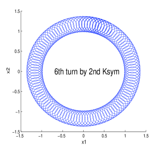
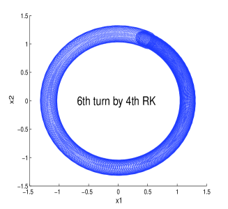
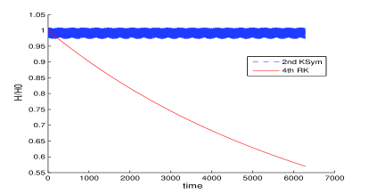
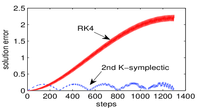
Figure 1: (a) Numerical orbits of the 2nd order K-symplectic method from the 190000-th step. (b) Numerical orbits of the 4th order RK method from the 190000-th step. (c) Energy error of the two methods as a function of the computing steps till the 20000-th step. (d) Solution error as a function of the computing steps, the step size in this sub-figure is $h=0.23\pi$.

In Fig. 1(a) and (b), numerical orbits of the two methods from the 190000-th step are plotted. Theoretical analysis shows that the particle’s orbit is a spiraling circle with constant radius, where the large circle corresponds to the drift of the guiding center, and the small circle is the fast-scale gyromotion. From Fig. 1(a) it is observed that after long computation time the 2nd order K-symplectic method still gives a correct orbit, while in Fig. 1(b) the 4-th order RK method fails because of the dissipated numerical gyromotion. This can be explained partly by their performances at the energy. The obvious energy damping by the 4nd order Runge-Kutta method is demonstrated in Fig. 1(c). On the contrary, the second order $K$ symplectic numerical method can bound the energy up to error $h^{2}$ (see Figs.1(c), 2(b)) which agrees with the theoretical error analysis. In Fig.1(d), we show the error growth of the numerical solution along with the simulation time. The step size is chosen to be $h=0.23\pi$. It can be seen that the error caused by the Runge-kutta method is smaller at the first few steps, but grows larger than that of the $K$-symplectic method rapidly.

Next, we study the accuracy and computing amount of the $K$-symplectic methods. Fig.2(a) displays the solution error as a function of the computing cost. When the requirement on solution error is smaller than $1\%$, the second order method needs less computing time and is more efficient than the first order method.

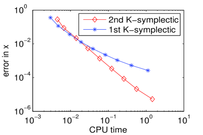
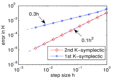
Figure 2: (a) Solution error as a function of the computing time. (b) Error of the numericl energy as a function of the step size $h$.

IV Conclusion

In this paper, we have constructed numerical methods for the Lorentz force system focusing on its $K$-symplectic structure. As there exists a Darboux transformation such that the $K$-symplectic structure can be turned into the standard symplectic structure, the error analysis for the canonical numerical methods can be generalized to the $K$-symplectic numerical methods. However, the Darboux transformation usually is not able to be expressed explicitly. Thus, it is generally not easy to design the $K$-symplectic numerical methods. For our study, we decompose successfully the Lorentz force system as four subsystems which can be solved explicitly. The resulting numerical methods by composing the exact solutions of the four subsystems naturally preserve the $K$-symplectic structure. The numerical experiment shows the superior long-term performances of the new derived numerical methods. More theoretical and numerical analysis of the K-symplectic methods will be reported in future publications. The splitting idea has been generalized to construct the numerical methods for the Vlasov-Maxwell equations in heqinsun15him .

References

- (1) Y. He, Y. Sun, J. Liu, H. Qin, Volume-preserving algorithms for charged particle dynamics, J. Comput. Phys. 281 (2015) 135–147.
- (2) Y. He, Y. Sun, J. Liu, H. Qin, Higher order volume-preserving schemes for charged particle dynamics, submitted.
- (3) R. I. McLachlan, G. R. W. Quispel, Splitting methods, Acta Numer. 11 (2002) 341–434.
- (4) S. A. Chin, Symplectic and energy-preserving algorithms for solving magnetic field trajectories, Phy. Rev. E 77 (2008) 066401.
- (5) E. Hairer, C. Lubich, and G. Wanner, Geometric Numerical Integration: Structure-preserving algorithms for ordinary differential equations, 2nd Edition, Springer-Verlag, Berlin, 2006.
- (6) Y. He, H. Qin, Y. Sun, J. Xiao, R. Zhang, J. Liu, Hamiltonian time integrators for Vlasov-Maxwell equations, submitted.