Transmission Properties of Branched Atomic Wires

1 Abstract

The renormalization-decimation method is used to study the transmittivity of atomic wires, with one or more side branches attached at multiple sites. The rescaling process reduces all the branches, attached at an atomic site, to an equivalent impurity, from which the transmission probability can be calculated using the Lippmann-Schwinger equation. Numerical results show that the subsequent $T(E)$ curves, where particular attention is paid to the numbers and locations of resonances and anti-resonances, are highly sensitive to the values of each system’s key parameters. These findings provide insight into the design of wires with specific desired properties.

2 Introduction

Modern fabrication techniques allow electronic devices to be designed and constructed at the molecular level. Consequently, it is instructive to investigate possible structures theoretically, with a view to their varying physical properties, as a guide to designing devices with the desired characteristics. Of interest here are the electronic transmission aspects of the atomic wire, and how they can be modified by the attachment of one or more atoms (or groups of atoms) at various points on the wire.

An early study, along these lines, was that of Guinea and Vergés [1], who investigated the electronic properties of a chain with linear side branches and loops. The work concentrated on the local densities of states, but also considered the implications for transmission. A key finding was that the irregularities in geometric structure lead to the blocking of transmission, at certain energies. A later treatment, focusing on transmisison through a chain, was performed by Singha Deo and Basu [2].They showed that an interplay between substitutional impurities and topological defects (such as a side branch) can make the band asymmetric, with resulting effects on the transmission. The effect can arise with as little as a single impurity present in an otherwise periodic chain. More recently, Kalyanaraman and Evans [3] also considered electron transfer along an atomic wire with a side branch, and with particular attention paid to dendritic structures. The main result was that such structures can exhibit larger conductance than linear chains, with the position and topology of the side branches being crucial in determining the transport properties. Farchioni et al [4] utilised the renormalization method (see, e.g., [5]) to study electron transmission through a ladder (two coupled chains) with a side-attached impurity, observing that the effects are quite different than for a substitutional impurity.

The present authors [6] used a tensorial Green-function method to study overlap effects on electron transmission through the simplest type of branched atomic wire, namely, a T-junction consisting of a chain of atoms with just a single additional atom attached to its side. It was observed that overlap can either enhance or suppress transmission, and does so in a different way than does the presence of an impurity or a branch in the chain.

The present paper extends the previous work [6] to consider more elaborate attachments, specifically, longer branches with sub-branches and multiple branches at a single site, and branches at two sites along the atomic wire. The method used is the tensorial Green-function technique of earlier work [6, 7], which allows for the inclusion of overlap both in the atomic wire and any attached structures. The renormalization method [5] provides an efficient way to treat a complicated attachment, by rescaling it to an energy-dependent substitutional impurity at the chain site to which the structure is attached. As we are considering such attachments at either one or two sites, such systems can thus be reduced to atomic wires with one or two impurities. As previously mentioned, the former has been considered by us [7], while the latter has only been treated in the zero-overlap case [8]. Thus, the methodology, discussed in the next sections, firstly extends the theory of electron transmission through double-impurity wires, so as to incorporate overlap, which is similar to the single-impurity theory, then, secondly, uses the renormalization technique to reduce complicated branched structures to single atomic wires containing one or two impurities.

3 Transmission through Double-impurity Wires, including Overlap

In this section, we look briefly at the theory of electron transmission through an atomic wire, with two impurities at a separation $d$, as shown in Figure 1.

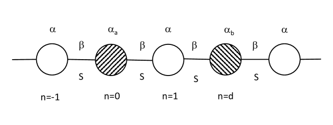
Figure 1: Atomic wire with 2 impurities, at separation $d$.

The wire is modelled by a linear chain of atoms, with $\alpha$ being the atomic-site energy, $\beta$ the bond energy, and $S$ the nearest-neighbour overlap. The impurities, at the sites $n=0$ and $n=d$, have modified site energies $\alpha_{a}$ and $\alpha_{b}$, respectively, with the obvious feature that the system reduces to a one-impurity chain by setting $\alpha_{b}=\alpha$. Transmission through such a wire for the case of no overlap ($S=0$) has been treated by Mišković et al [8], from which the extension to the case $S\neq 0$ is straightforward, using the method of reference [7]. To this end, with some changes in notation, the Mišković equation (21) for the transmission probability becomes

$$T(E)=|\tau|^{2}=|(1-ic_{a})(1-ic_{b})+c_{a}c_{b}t^{2d}|^{-2},$$ (1)

where

$$c_{k}=s(\alpha_{k}-\alpha)(1-\xi^{2})^{-1/2}/(4\beta Y)~{},~{}k=a~{}{\rm or}~{}b,$$ (2)

and

$$t=\left\{\begin{array}[]{ll}\xi+s(\xi^{2}-1)^{1/2},&|\xi|>1,\\ \xi+is(1-\xi^{2})^{1/2},&|\xi|<1,\\ \end{array}\right.$$ (3)

with

$$s=\pm 1~{}{\rm so~{}that}~{}|t|<1.$$ (4)

Here,

$$\xi=X/2Y=(E-\alpha)/2(\beta-ES),$$ (5)

where

$$X=(E-\alpha)/2\beta,$$ (6)

and

$$Y=(1-\alpha S/\beta-2SX)/2.$$ (7)

The fundamental mathematical change in including overlap is that the bond energy $\beta$ is replaced by the energy-dependent quantity $\beta-ES$. Conversely, if overlap is removed by setting $S=0$, then the above results reduce to those of [7].

4 Renormalization Technique

The renormalization technique [5] provides an efficient avenue to investigate complicated structures, by rescaling them into simpler ones, with one or more parameters becoming energy-dependent. Although the method is most commonly used without inclusion of overlap, it is straightforward to do so. We here illustrate the method by looking at its application to the simplest system of interest in this paper, namely a linear chain with a single extra atom attached at the side of site 0 (see Figure 2(a)).

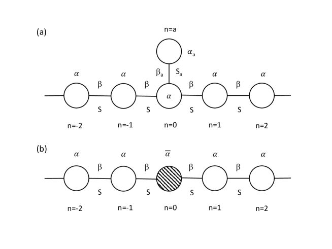
Figure 2: (a) Chain with one side-atom attached. (b) Rescaled chain with side-atom deleted.

The pure chain is as described in the last section, while the side-atom has a site energy $\alpha_{a}$, bond energy $\beta_{a}$ and overlap $S_{a}$. Within the tight-binding approximation, the discretized Schrödinger equation takes the well-known form [7] of a set of second-order difference equations, which for the system under consideration is:

$$(E-\alpha)c_{n}=(\beta-ES)(c_{n-1}+c_{n+1})~{},~{}n\neq 0,a,$$ (8)

$$(E-\alpha)c_{0}=(\beta-ES)(c_{-1}+c_{1})+(\beta_{a}-ES_{a})c_{a},$$ (9)

$$(E-\alpha_{a})c_{a}=(\beta_{a}-ES_{a})c_{0}.$$ (10)

Renormalization proceeds by eliminating $c_{a}$ from the set. Equation (10) can be solved as

$$c_{a}={(\beta_{a}-ES_{a})\over(E-\alpha_{a})}c_{0},$$ (11)

which, when substituted into (9), produces

$$(E-\bar{\alpha})c_{0}=(\beta-ES)(c_{-1}+c_{1}),$$ (12)

where

$$\bar{\alpha}=\alpha+{(\beta_{a}-ES_{a})^{2}\over(E-\alpha_{a})}$$ (13)

is the renormalized site energy. Thus, equation (10) has been eliminated, leaving the system of equations as (8) along with (12), and represented schematically by Figure 2(b). The procedure can be extended to more complicated systems, as will be seen in the next section, by eliminating sites, one-by-one, starting at the end of a branch, which corresponds mathematically to recursive application of (13) to produce the renormalized site energy at the “root” site, which appears as an impurity in the chain.

5 Application to Branched Atomic Wires

5.1 Chain with Branch and Sub-branch

We now proceed to investigate electron transmission through certain branched atomic-wire systems, by using the renormalization method to reduce such systems to linear chains with one or two impurities, whose transmission is then given by (1). The first system under study is an atomic wire with a single side branch, which itself has a sub-branch (see Figure 3(a)).

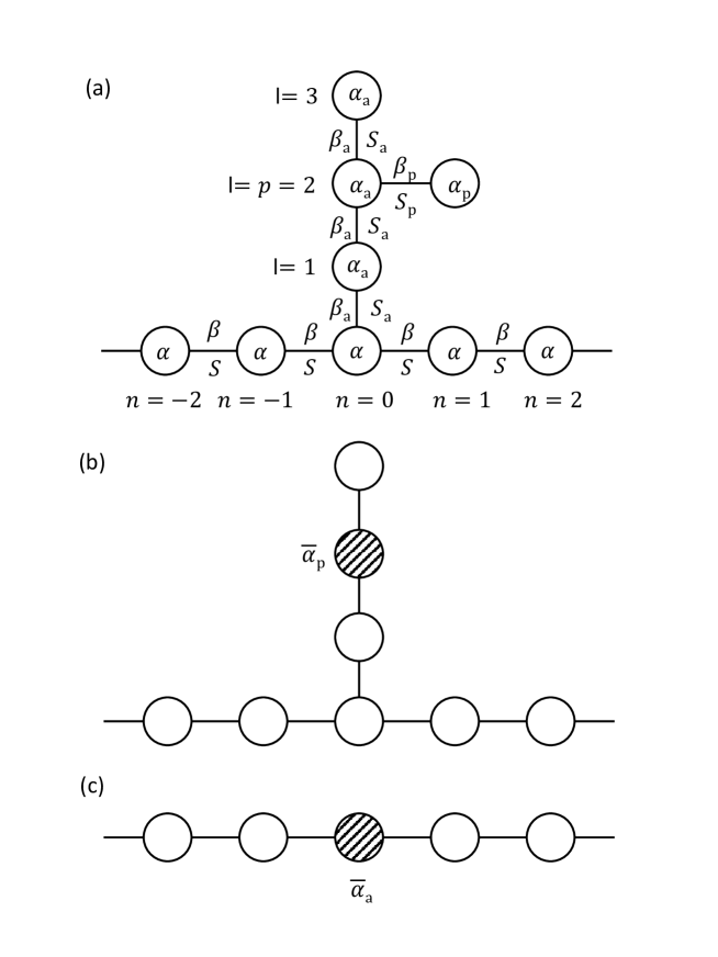
Figure 3: (a) Chain with one branch plus side-atom. (b) Result of first renormalization. (c) Final result of renormalization process.

The branch is of length $l_{a}$, and is attached to the main wire at site $n=0$. Each atom in the side branch has site energy $\alpha_{a}$, bond energy $\beta_{a}$ and overlap $S_{a}$. The sub-branch is attached to the primary branch at site $l=p$, and, for simplicity, the sub-branch is taken to consist of just a single atom, although the generalization to a longer sub-branch is straightforward. The atom comprising the sub-branch is taken to have site energy $\alpha_{p}$, bond energy $\beta_{p}$ and overlap $S_{p}$. The first step in the renormalization process is to delete the sub-branch atom, resulting in a rescaled atom at site $l=p$ (Figure 3(b)), whose site energy, using (13), is

$$\bar{\alpha}_{p}=\alpha_{a}+{(\beta_{p}-ES_{p})^{2}\over(E-\alpha_{p})}.$$ (14)

The second step is to decimate the branch, atom by atom, starting at the free end ($l=l_{a}$), through repeated application of (13), resulting in only a chain with a rescaled atom at site $n=0$ (Figure 3(c)), whose site energy can be written in continued-fraction form as

$$\bar{\alpha}_{a}=\alpha+{(\beta_{a}-ES_{a})^{2}\over E-\alpha_{a}-}~{}{(\beta_{a}-ES_{a})^{2}\over E-\alpha_{a}-}\cdots{(\beta_{a}-ES_{a})^{2}\over E-\bar{\alpha}_{p}-}\cdots{(\beta_{a}-ES_{a})^{2}\over E-\alpha_{a}},$$ (15)

where the term $\bar{\alpha}_{p}$ occurs at position $p$ (counting from the left end of the continued fraction). Alternatively, (15) can be expressed more compactly using Gauss’ notation as

$$\bar{\alpha}_{a}=\alpha-{\rm K}_{l=1}^{l=l_{a}}\Big{[}{-(\beta_{a}-ES_{a})^{2}\over E-\alpha_{l}}\Big{]},$$ (16)

where

$$\alpha_{l}=\left\{\begin{array}[]{ll}\alpha_{a},&l\neq p,\\ \bar{\alpha}_{p},&l=p.\\ \end{array}\right.$$ (17)

Hence, the transmission can be calculated as that through a 1-impurity wire, by using equations (1)-(7), with $\alpha_{a}\rightarrow\bar{\alpha}_{a}$ and $\alpha_{b}\rightarrow\alpha$.

5.2 Chain with Multiple Branches at One Site

Next, we turn to the system of an atomic wire with $M$ branches attached at the same site ($n=0$), as shown in Figure 4.

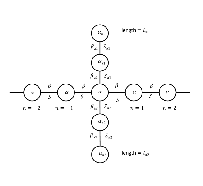
Figure 4: Chain with side branches at one site.

On branch $m$ ($=1,...,M$), which is of length $l_{m}$, the atoms have site energy $\alpha_{am}$, bond energy $\beta_{am}$ and overlap $S_{am}$. Each branch can be decimated via the renormalization procedure, as was done in the previous subsection, albeit without sub-branches attached. Consequently, each branch contributes to $\bar{\alpha}_{a}$ a continued fraction of the form appearing in (16), resulting in the rescaled site-energy at site $n=0$ being

$$\bar{\alpha}_{a}=\alpha-{\textstyle\sum_{m=1}^{m=M}}\Big{(}{\rm K}_{l=1}^{l=l_{m}}\Big{[}{-(\beta_{am}-ES_{am})^{2}\over E-\alpha_{am}}\Big{]}\ \Big{)}.$$ (18)

Thus, as in the last subsection, the transmission is through a rescaled 1-impurity wire, with $\alpha_{a}\rightarrow\bar{\alpha}_{a}$ and $\alpha_{b}\rightarrow\alpha$.

5.3 Chain with Branches at Two Sites

The last system under investigation is an atomic wire, with a pair of branches attached at sites $n=0$ and $n=d$ (see Figure 5).

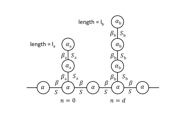
Figure 5: Chain with side branches at two sites, at separation $d$.

The branches are of lengths $l_{a}$ and $l_{b}$, respectively, and have associated site energies $\alpha_{k}$, bond energies $\beta_{k}$ and overlaps $S_{k}$, with $k=a~{}{\rm or}~{}b$. Each branch can be decimated, atom by atom, as in the preceding subsections by the repeated application of (13). Consequently, sites 0 and $d$ of the chain become occupied by rescaled atoms with site energies

$$\bar{\alpha}_{k}=\alpha-{\rm K}_{l=1}^{l=l_{k}}\Big{[}{-(\beta_{k}-ES_{k})^{2}\over E-\alpha_{k}}\Big{]},~{}k=a~{}{\rm or}~{}b,$$ (19)

respectively. Hence, the transmission $T(E)$ can be calculated, via (1), as that through a 2-impurity wire, with $\alpha_{a}\rightarrow\bar{\alpha}_{a}$ and $\alpha_{b}\rightarrow\bar{\alpha}_{b}$.

6 Results and Discussion

We now proceed to examine the $T(E)$ curves for the three systems, for some specific values of the various parameters. In order to provide some degree of uniformity, we take as “standard” values, all site energies $\alpha$’s to be 0, bond energies $\beta$’s to be -0.5 and overlaps $S$’s to be 0.25, except as otherwise stated.

Turning first to the system of a chain with one branch plus a side-atom, the key parameters to investigate are the length of the branch $l_{a}$ and the postion $p$ of the side-atom on that branch. With respect to the former, Figure 6 shows the $T(E)$ graphs for several branch lengths, with the side-atom set at position $p=1$, i.e., attached to the branch-atom closest to the main chain.

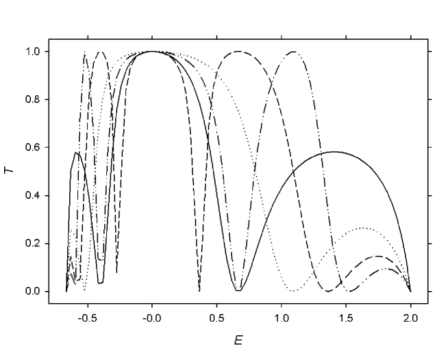
Figure 6: $T(E)$ for chain with branch, plus side-atom attached at position $p=1$. The branch is of length $l_{a}=$ (a) 1 (solid curve), (b) 2 (dotted), (c) 3 (dashed), (d) 4 (dash-dotted).

Starting with the case $l_{a}=1$ (Figure 6(a)), we see a single resonance ($T=1$) at $E=0$, flanked by a pair of anti-resonances ($T=0$), which separate the central peak from two smaller ones nearer the band edges. By comparison, $T(E)$ for a chain with a branch, but no side-atom, shows one resonance and just a single anti-resonance (see Figure 2 of [6]), while that for a bare chain, with no branch, shows only the single resonance and no anti-resonances at all (see Figure 5 of [7]). Moving to a branch of length $l_{a}=2$ (Figure 6(b)), we see a very similar $T(E)$ curve, namely, a large central peak with resonance at $E=0$, with 2 smaller peaks at the sides, albeit with the 2 anti-resonances shifted somewhat outwards, towards the band edges. However, further lengthening of the branch to $l_{a}=3$ (Figure 6(c)) produces a very different $T(E)$ curve, in which the central peak has split into 3, each achieving a resonance, while the 2 outermost peaks are further diminished, and also narrowed, by virtue of their bounding anti-resonances again moving further outwards. These features are repeated in the next longer branch ($l_{a}=4$ in Figure 6(d)), but once more with all anti-resonances moving outwards. This pattern is repeated as the branch is further lengthened (graphs not shown), with pairs of graphs for branch lengths $2m-1$ and $2m$ appearing very similar, but with an additional pair of anti-resonances appearing, due to a split of the central peak, in going to lengths $2m+1$ and $2m+2$.

The dependence of the $T(E)$ curves, on the position $p$ of the side-atom on the branch, is illustrated in Figure 7, for a branch of length $l_{a}=4$.

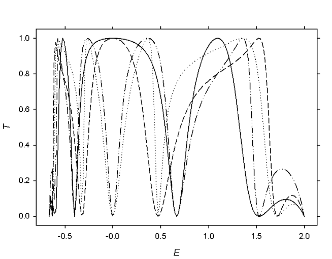
Figure 7: $T(E)$ for chain with branch of length $l_{a}=4$, plus side-atom attached at position $p=$ (a) 1 (solid curve), (b) 2 (dotted), (c) 3 (dashed), (d) 4 (dash-dotted).

The graph for $p=1$ (Figure 7(a)), it should be noted, is that appearing in Figure 6(d), again showing the structure of 5 peaks, 3 of them resonances, divided by 4 anti-resonances. When the side-atom is moved outwards along the branch to position $p=2$ (Figure 7(b)), the central resonance, centered at $E=0$, is split into a pair of narrower resonances, accompanied by some shifting of the anti-resonances, so as to broaden the other 2 resonances. As the side-atom is moved again to $p=3$ (Figure 7(c)), however, these 2 new resonances recombine into a single one at $E=0$, with the 2 outer resonances relatively unchanged. The graph now looks very similar to that for $p=1$ in Figure 7(a), in terms of number of resonances and anti-resonances, except that the central resonance peak has been narrowed, allowing broadening of the outer two. With an increase to $p=4$ (Figure 7(d)), the central resonance agains splits into a pair of resonances. This pattern repeats itself, on branches of arbitrary length, as $p$ increases, namely, the number of resonances oscillates as the central resonance splits in two and then recombines.

A detailed mathematical analysis can reveal much about the features seen in Figures 6 and 7 and, in particular, about the dependance on the parameters of the number of anti-resonances, which largely determines the overall structure of the graphs. Referring to equation (1), it can be seen that in order for an anti-resonance to occur, i.e., $T=0$, it is necessary that $c_{l}\rightarrow\pm\infty$. Looking at (2), $\alpha_{b}\rightarrow\alpha$ (as indicated in section 5.1) giving $c_{b}=0$, thus leaving only $c_{a}$ to consider. For $c_{a}\rightarrow\pm\infty$ in (2) requires that $\bar{\alpha}_{a}-\alpha\rightarrow\pm\infty$, as it can be shown that $Y\neq 0$ and $1-\xi^{2}=0$ only at the band edges (where T always equals 0, so these two energies are not considered to be anti-resonances). Thus, anti-resonances correspond to singularities of $\bar{\alpha}_{a}-\alpha$, which can be located by analyzing (16), with the result that the maximum, and “usual”, number of anti-resonances equals $l_{a}+1$, namely, the total number of atomic sites in the entire side-structure (branch plus side-atom). However, for some parameter values, symmetry considerations can cause a coalescence of 2 anti-resonances, in a situation reminiscent of degeneracy. Suppose $\alpha_{a}=\alpha_{p}$, as is the case here. If, for example, $p=l_{a}-1$, then the side-structure has a symmetrical Y-shape, which results in the coalescence of 2 anti-resonances, thus dropping the total number to just $l_{a}$. This feature does not happen when $p=l_{a}$ or $l_{a}-2$. It depends upon the parity (even or odd) of $p$ compared to that of $l_{a}$, and it turns out that the number of anti-resonances is $l_{a}+1$ when $p$ and $l_{a}$ have the same parity, but the number drops to $l_{a}$, when they have opposite parity. It should be noted that, if $\alpha_{a}\neq\alpha_{p}$, then the symmetry consideration does not hold, and the number of anti-resonances is $l_{a}+1$. These considerations explain the basic structure of the two figures. Firstly, in Figure 6, increasing $l_{a}$, while holding $p$ constant, switches the parity back and forth, resulting in pairs of graphs, with branch lengths $2m-1$ and $2m$, having the same number of anti-resonances. Secondly, in Figure 7, increasing $p$, while holding $l_{a}$ constant, also flips the parity, causing the number of anti-resonances to oscillate up and down.

Turning next to the system of a chain with multiple branches attached at one site, the most important parameters are the number of branches $M$ and their lengths $l_{m}$. The variation of $T(E)$ with the number of branches is illustrated in Figure 8, for branches of length 2.

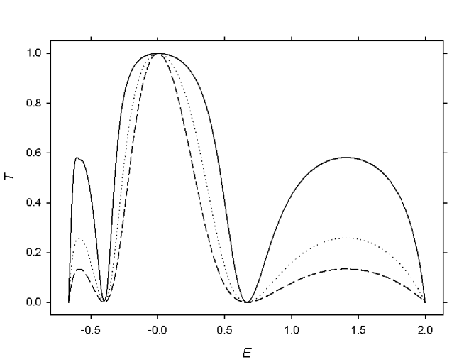
Figure 8: $T(E)$ for chain with branches of length $l_{m}=2$, the number of branches being $M=$ (a) 1 (solid curve), (b) 2 (dotted), (c) 3 (dashed).

For only a single branch (Figure 8(a)), $T(E)$ shows a single resonance peak at $E=0$, with a pair of smaller peaks to the sides, separated by a pair of anti-resonances, at $E=-0.4$ and $E=0.65$. Adding a second branch produces a similar $T(E)$ curve (Figure 8(b)), in that the resonance and the two anti-resonances persist at their previous energies. However, there is a general dampening of the transmission, resulting in lower $T(E)$ at all energies, except the resonance. This effect is enhanced with the addition of a third branch (Figure 8(c)), where transmission is further suppressed, but with the resonance and both anti-resonances preserved. In the more general situation, where atoms on different branches have different site energies ($\alpha$’s), more anti-resonances (and, hence, more peaks) appear, but the addition of more branches again has the overall effect of lowering transmission. Thus, we make the general observation that more branches is inhibitive to transmission.

The dependence of $T(E)$ on the length of branches is shown in Figure 9, where the number of branches is taken to be 3.

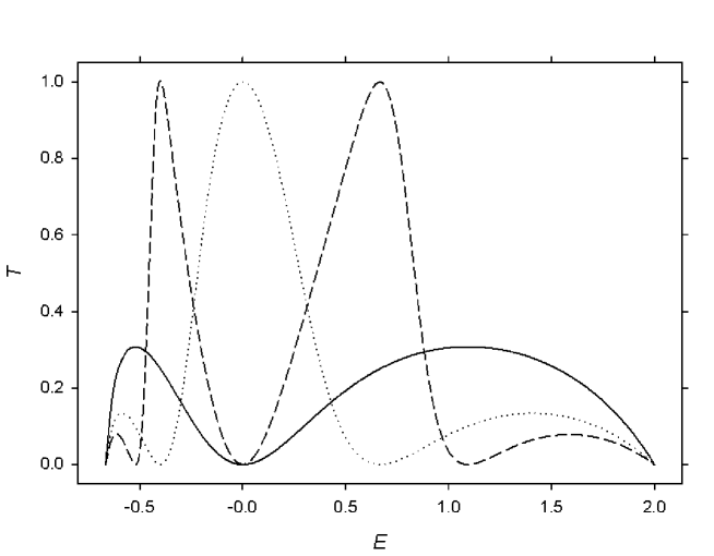
Figure 9: $T(E)$ for chain with $M=3$ branches, all of length $l_{m}=$ (a) 1 (solid curve), (b) 2 (dotted), (c) 3 (dashed).

For branches of length 1 (i.e., they are individual atoms), the $T(E)$ curve (Figure 9(a)) shows relatively low transmission at all energies, with a single anti-resonance at $E=0$ separating two small peaks. Increasing the lengths of the branches to 2 produces a markedly different structure (Figure 9(b)), in which a central peak, with a resonance at $E=0$, appears, with 2 much smaller peaks to the sides, and a pair of anti-resonances separating them from the central peak. A further increase of the branch lengths to 3 (Figure 9(c)) produces a third anti-resonance, with the 2 central peaks now becoming resonances, and the 2 outside peaks showing even lower transmission. This trend continues as the chains are further lengthened, with additional anti-resonances appearing and all the resulting peaks, except the 2 outer ones, showing resonances. As an individual branch is lengthened (graphs not shown), the number of anti-resonances increases in a pattern similar to that noted earlier, in the discussion of Figure 6.

Much of the basic structure of this system can be illuminated by, as before, analyzing the number of anti-resonances, as illustrated in Figures 8 and 9. As with the first system, anti-resonances are calculated as singularities of $\bar{\alpha}_{a}-\alpha$, now using (18). The main result from earlier is still valid, namely, that the maximum number of anti-resonances arising from a branch equals the length $l_{m}$ of the branch. Thus, for a system with $M$ branches, the maximum number of anti-resonances in the system equals $l_{1}+\cdots+l_{M}$. However, for the parameter values used here, where each branch is assumed to have identical atoms, so that corresponding parameters ($\alpha_{am}$, etc,) are equal, the number of anti-resonances may turn out to be less than the maximum. In particular, if the branches all have equal length, as is the case in Figures 8 and 9, then the anti-resonances arising from one branch coincide with those from the other branches, so that the number of anti-resonances equals the common branch length $l_{m}$. But if the branch lengths are unequal, then typically the anti-resonances from different branches do not coincide, and there is no reduction in total number from the maximum.

Lastly, turning to the system of a chain with a pair of branches, at separate sites, the significant parameters are the separation $d$ between the two branches, and their lengths $l_{a}$ and $l_{b}$. The variation of $T(E)$ with the separation between branches is shown in Figure 10, for branches of fixed lengths 1 and 3.

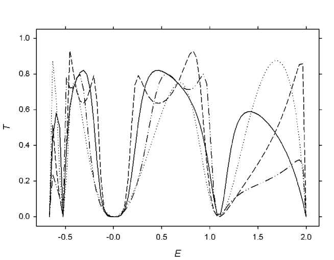
Figure 10: $T(E)$ for chain with 2 branches, of lengths $l_{a}=1$ and $l_{b}=3$, and at separation $d=$ (a) 1 (solid curve), (b) 2 (dotted), (c) 3 (dashed), (d) 4 (dash-dotted).

(It should be noted that $T(E)$ is invariant to interchange of the lengths $l_{a}$ and $l_{b}$.) When the branches are attached to adjacent sites in the chain, corresponding to $d=1$ (Figure 10(a)), the $T(E)$ curve shows a structure which is quasi-symmetric about $E=0$. (In the case where there is no overlap, the curve is precisely symmetric.) There are 3 anti-resonances, including one at $E=0$, which divide the band region into 4 zones of transmission, albeit with no resonances. As the separation increases (Figure 9(b-d)), the number and positions of the anti-resonances do not change, leading to a very similar graph for $d=2$, but to noticeably different ones for $d=3$ and 4, where the inner pair of peaks exhibit some rearrangement to produce double-peaked structures, while the outer pair are greatly diminished, at least for $d=4$. For further increases in separation (graphs not shown), the three anti-resonances remain pinned at their energy values, while the transmittivity continues to be dominated by the inner pair of sub-bands, which gradually add extra peaks within each zone.

The variation of $T(E)$ with branch length is exemplified by Figure 11, where the length $l_{b}$ of one branch is varied, while the other $l_{a}=1$ is held constant, with fixed separation $d=2$.

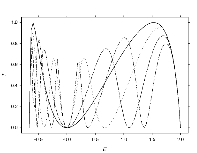
Figure 11: $T(E)$ for chain with 2 branches, at separation $d=2$, and lengths $l_{a}=1$ and $l_{b}=$ (a) 1 (solid curve), (b) 2 (dotted), (c) 3 (dashed), (d) 4 (dash-dotted).

For the shortest branch $l_{b}=1$ (Figure 11(a)), there is a single anti-resonance at $E=0$ separating two bands of transmission, with resonances at about $E=-0.5$ and $E=1.5$. The asymmetry, produced by the presence of overlap, distorts the $T(E)$ curve, so that the part of the band most amenable to transmission is at the higher energies. As the branch is lengthened to $l_{b}=2$ (Figure 11(b)), each region of transmission is split into two by the creation of a pair on anti-resonances, while the heights of all 4 peaks are lowered, so as to remove both resonances. The result, then, is an overall weakening of the transmittivity of the wire, except at certain energies. Lengthening the branch again to $l_{b}=3$ (Figure 11(c)) produces a graph very similar to the previous one, with the same number of anti-resonances and peaks, but with some shifting of their energies (except, noticeably, the anti-resonance at $E=0$). However, a further lengthening of the branch to $l_{b}=4$ creates a splitting of the two inner peaks (Figure 11(d)), for a total of 6, separated by 5 anti-resonances (including the fixed one at $E=0$). The net effect is an overall lowering of the transmittivity, except at and near the peaks. The structure in the graph for $l_{b}=4$ persists at $l_{b}=5$ (not shown), but when $l_{b}=6$, there is a further splitting of the innermost pair of peaks, accompanied by the appearance of an extra pair of anti-resonances. Thus, we see a pattern that is reminiscent of that observed with the lengthening of branches in the two earlier systems.

An analysis of the anti-resonances follows similar lines to that presented for the other two systems, but now utilizing (19). First, we note that the number and positions of anti-resonances are independent of the separation $d$ between the two branches, as can be seen in Figure 10. In general, there are anti-resonances associated with each branch, the number being equal to the length of the branch, so that the maximum number of anti-resonances is $l_{a}+l_{b}$. However, as in the earlier systems, taking corresponding parameters on the two branches to be equal, typically reduces the actual number of anti-resonances. Specifically, this reduction occurs when $l_{a}$ and $l_{b}$ are both odd, which results in $E=\alpha_{a}=\alpha_{b}$ being an anti-resonance energy for both branches, thus reducing the total number, by 1, to $l_{a}+l_{b}-1$. For certain other combinations of lengths, the total number of anti-resonances can also be reduced. A special situation occurs when $l_{a}=l_{b}$, with corresponding parameters equal, so that the two branches are identical. In this case, the number of anti-resonances equals the common length $l_{a}$. These considerations explain the pattern of anti-resonances seen in Figure 11.

7 Conclusion

Starting from the bare atomic wire, more complicated electronic systems can be built, by adding one or more side branches, at one or more sites, along the wire. By examining these different structures, we can gain insight into those variations which produce the most useful properties. The present work utilizes the renormalization-decimation method, whereby all the side branches, attached to a particular site, were reduced to an impurity replacing the original atom at that site. Subsequently, the transmission probability $T(E)$ through the wire was calculated by means of the established Lippmann-Schwinger technique.

In all of the three systems examined, the key to understanding the $T(E)$ curve lies in the number and positions of anti-resonances and resonances (or smaller maxima). These in turn can be varied and controlled by means of the system’s main parameters, such as the length of a side branch, thus indicating that the wire can be constructed to have a fairly specific $T(E)$ profile, through a judicious choice of the attached structures.

It is interesting to note that the results of the present study indicate that the renormalization-decimation technique may be a useful tool in the area of chemisorption. For example, it could be used to investigate the chemisorption properties of a molecule adsorbed onto an atomic wire, by treating the admolecule similarly to the side-structures of this paper. In such a case, the admolecule can be renormalized down to a single impurity in the wire, thus simplifying the chemisorption calculation.

8 Keywords

Branched atomic wires, molecular electronics, renormalization-decimation technique, semi-empirical calculations

References

- [1] F. Guinea, J.A. Vergés, Phys. Rev. B 1987, 35, 979.
- [2] P. Singha Deo, C. Basu, Phys. Rev. B 1995, 52, 10685.
- [3] C. Kalyanaraman, D.G.Evans, Nano. Lett. 2002, 2, 437.
- [4] R. Farchioni, G. Grosso, G.P. Parravicini, Eur. Phys. J. B 2011, 84, 227.
- [5] R. Farchioni, G. Grosso, P. Vignolo, Organic Electronic Materials, (Eds. R. Farchioni, G. Grosso), Springer, Berlin, 2001, pp. 89-125.
- [6] K.W. Sulston, S.G. Davison, Int. J. Qu. Chem. 2013, 113, 1498.
- [7] K.W. Sulston, S.G. Davison, Phys. Rev. B 2003, 67, 195326.
- [8] Z.L. Mišković, R.A. English, S.G. Davison, F.O. Goodman, Phys. Rev. B, 1996, 54, 255.