Jet-Medium Interactions at NLO in a Weakly-Coupled Quark-Gluon Plasma

Abstract

We present an extension to next-to-leading order in the strong coupling constant $g$ of the AMY effective kinetic approach to the energy loss of high momentum particles in the quark-gluon plasma. At leading order, the transport of jet-like particles is determined by elastic scattering with the thermal constituents, and by inelastic collinear splittings induced by the medium. We reorganize this description into collinear splittings, high-momentum-transfer scatterings, drag and diffusion, and particle conversions (momentum-preserving identity-changing processes). We show that this reorganized description remains valid to NLO in $g$, and compute the appropriate modifications of the drag, diffusion, particle conversion, and inelastic splitting coefficients. In addition, a new kinematic regime opens at NLO for wider-angle collinear bremsstrahlung. These semi-collinear emissions smoothly interpolate between the leading order high-momentum-transfer scatterings and collinear splittings. To organize the calculation, we introduce a set of Wilson line operators on the light-cone which determine the diffusion and identity changing coefficients, and we show how to evaluate these operators at NLO.

1 Introduction

Jets are a key observable in the relativistic heavy-ion program Roland:2014jsa ; d'Enterria:2009am ; Majumder:2010qh ; Mehtar-Tani:2013pia . Advances in reconstructing jets at the LHC Aad:2010bu ; Chatrchyan:2011sx challenge our ability to understand the difference between jet development in the hot medium created in a heavy ion collision, compared to development in the vacuum or near-vacuum environment of a proton-proton collision. While early theoretical studies concentrated on understanding the leading hadron in a jet (see ref. Burke:2013yra for an overview), the more inclusive jet reconstructions which are now possible experimentally demand a theoretical description of the full jet evolution, including the evolution of all radiated daughters.

Several groups have put forward modeling frameworks for doing this Majumder:2013re ; Zapp:2011ya ; Schenke:2009gb ; Renk:2010zx ; Armesto:2009fj . It is fair to say that these approaches have some commonalities. Generally they separate the excitations into high-energy partons associated with the jet, and low-energy partons or a scattering medium with a characteristic energy scale $T$ (the local medium temperature). Then, one attempts to follow the evolution of the high energy partons, which will eventually create the hadrons reconstructed as a jet. The jet partons are considered to interact with the medium in two important ways. They scatter elastically, and they are induced to radiate or split. Different frameworks differ in whether both possibilities are considered, and in exactly how the splitting processes are computed (how is long-distance coherence handled? Is the radiated daughter assumed to have a small fraction of the energy? What model for the medium interactions, and what other approximations are made?).

Typically the division of processes into distinct types – here elastic scattering and inelastic radiation – is justified at leading order, but at subleading orders they often cannot be clearly distinguished. What happens to the treatment of jet-medium interaction at subleading order? Is it possible to pursue a next-to-leading order (NLO) calculation, in the sense that the elastic and splitting interactions between the jet partons and the medium are treated beyond leading perturbative order? In this paper we explore this question by extending a framework where it is clearly posed – the AMY/McGill/MARTINI approach Arnold:2002ja ; Arnold:2002zm ; Jeon:2003gi ; Qin:2007rn ; Schenke:2009ik ; Schenke:2009gb , where there is a clear power-counting prescription for determining what is leading and subleading order for the jet-medium interaction. The approach starts with the assumptions that the medium is thermal and weakly coupled, so the interactions between jet partons and the medium can be computed in thermal perturbation theory. One also assumes that the medium is thick, such that the formation times of processes under consideration are shorter than the scale of variation of the medium. This approximation has sometimes been criticized, and it can be improved upon without overturning the rest of the approach CaronHuot:2010bp . But for the processes which will be most interesting here – processes involving small momentum transfer or intermediate opening angles – the scattering or formation times are relatively short, so this should be considered a separate issue.

The philosophy of the framework is as follows. We follow one or more “hard” approximately on shell partons traversing the medium. We assume that the medium has a local temperature $T\gg\Lambda_{\mathrm{QCD}}$, and distinguish a parton as hard if its energy $E$ satisfies $\exp(-E/T)\ll 1$. Particles failing this criterion are assumed to join the thermal medium; but no attempt is made to track the back-reaction on the medium properties Iancu:2015uja .

The jet parton evolution and jet-medium interactions are dictated by finite temperature perturbation theory. Whereas vacuum perturbation theory is an expansion in the strong fine-structure constant $\alpha_{\mathrm{s}}=g^{2}/4\pi$, this expansion is spoiled by soft-particle statistical functions $n_{\scriptscriptstyle B}(\omega\sim gT)\sim 1/g$ entering in thermal Feynman graphs. These soft contributions must be resummed to obtain a finite leading order answer, and give rise to subleading corrections suppressed by a single power of $g$. We have recently shown how to compute these subleading corrections in the context of hard real Ghiglieri:2013gia and virtual Ghiglieri:2014kma photon production. Here we extend that treatment to the case of jet-medium interactions.

As a scattering environment, the essential attribute of QCD (or any gauge theory) is that there is a large cross section for small-momentum-transfer scattering processes. These are responsible for the high rate of particle splitting. They also cause complications when including elastic scattering, since they give a large rate of small momentum exchanges, both in the transverse and longitudinal components of the momentum. At next-to-leading (NLO) order, new processes arise, which can be understood physically as overlap and interference between sequential scattering processes and as scatterings with the emission or absorption of soft ($E\sim gT$) excitations simonguy . These contribute both to transverse momentum broadening and to longitudinal momentum loss and broadening. They are most easily computed in a way which does not cleanly separate them into elastic and inelastic processes, and indeed it is not clear that the distinction is important or well posed. And they overlap with the infrared limits of both the elastic scattering and the splitting processes. However, frequent and small momentum exchanges need not be separately identified and tracked. In traversing enough medium to significantly modify a jet, the jet partons will undergo several such soft processes, in which case a statistical description should be sufficient. This motivates an approach in which we give a Fokker-Planck (Langevin) description of soft scatterings, as drag and diffusion processes.

The philosophy of our approach will therefore be the following. We will introduce infrared scales $\mu_{\perp}$, $\mu_{\parallel}$. All scattering and emission processes which change a jet parton’s momentum by more than $\mu_{\perp,\parallel}$ will be handled explicitly. All processes which change momentum by less than this scale, including the NLO effects alluded to above, will be incorporated as momentum diffusion and drag coefficients, which can be neatly defined in field theory as correlators of field strength operators on light-like Wilson lines. We will compute these drag and diffusion coefficients at the NLO level, as well as providing an NLO accurate procedure for computing the larger-transfer elastic and splitting processes. We will show explicitly how to perform a matching so that the choice of the scale $\mu$ drops out in the final results.

The drag and diffusion coefficients account for momentum exchange with the medium through soft gauge-boson exchange. Soft fermion exchange with the medium can change the identity of a quark to a gluon and vice versa. We call such identity changing processes conversion processes, and introduce a medium coefficient (analogous to the transverse momentum broadening coefficient $\hat{q}$ or the energy loss $\hat{e}$) which parameterizes this conversion rate. As with the drag and diffusion coefficients, all identity changing scattering processes with momentum exchange greater than $\mu$ will be treated explicitly, while identity changing scatterings with small momentum transfer are incorporated into the conversion rate. The conversion rate will be defined as a correlator of soft fermionic operators on light-like Wilson lines.

The calculation of the processes involving soft momentum transfers (drag, diffusion, and conversions) and of the corresponding light-cone Wilson line correlators requires a resummation scheme known as the Hard Thermal Loop (HTL) effective theory Braaten:1989mz ; Braaten:1991gm , which is the QCD analog of the Vlasov equations Blaizot:2001nr . These formalisms are well known to be computationally complex, and at first sight, any calculation beyond leading order in the coupling would seem extremely challenging (see simonguy for an example). However, Caron-Huot has shown CaronHuot:2008ni that HTL correlators (and statistical correlators more generally) simplify greatly when computed at light-like separations, which are exactly those that must be evaluated to determine the energy loss, diffusion, conversion, and collinear radiation rates of highly energetic particles propagating in a plasma.

Intuitively, these simplifications can be seen to arise because the energetic partons are propagating almost exactly along the light cone. Hence they are probing an essentially undisturbed plasma, at least as far as the soft, classical background is concerned. Informally, we can say that this background “can’t keep up” with the hard particles traversing the plasma. Thus, the soft correlations that the latter probe are statistical in nature rather than dynamical. Those simplifications, as we shall show, are at the base of the NLO extension being presented.

A pedagogical review of these recent developments in the understanding of HTLs has been presented by two of us in Ghiglieri:2015zma . There the main results of this paper, i.e. the reorganization of the kinetic theory we have mentioned, as well as the results of the computations to NLO of the needed rates and coefficients, have been partly anticipated. Due to the review nature of Ghiglieri:2015zma , the presentation there has been more pedagogical and most details and technical aspects have been omitted for the sake of brevity and clarity. Here we will present the detailed derivation of the reorganization of the kinetic approach, as well as the explicit calculations of the coefficients and rates. Furthermore, Ghiglieri:2015zma was limited to a plasma of gluons only, again for ease of illustration. We advise readers unfamiliar with Hard Thermal Loops, and especially with the recent developments discussed before, to explore Ghiglieri:2015zma first.

The paper is organized as follows: in Sec. 2 we present the LO framework in the standard formulation, which divides into elastic (${2\leftrightarrow 2}$) and inelastic (${1\leftrightarrow 2}$) processes. Readers familiar with that approach can skip directly to Sec. 3, where we introduce our reorganization in terms of large-angle scatterings, diffusion, conversion and collinear processes. In Sec. 4 we give an overview of the NLO corrections, which are dealt with in detail in Sec. 5 for collinear processes, Sec. 6 for diffusion, Sec. 7 for conversion and finally Sec. 8 for the semi-collinear processes, which first contribute at NLO and smoothly interpolate between the other three. A summary is presented in Sec. 9, together with our conclusions. Extensive technical details are to be found in the appendices, such as the NLO calculation of longitudinal momentum diffusion.

The paper is rather long and detailed. Some readers will be more interested in learning how to apply its results to their own (numerical) treatment of jet modification, without necessarily following all the details. In the online version of the paper, we have put boxes around the key equations which must be included in an implementation of our results. These readers can skip most of the text and focus on these boxed equations.

2 The leading-order kinetic approach

Our aim is to track the time evolution of a small number of highly-energetic jet-like particles as they propagate through a medium. We will refer to energies and momenta of order $E$ as hard, of order $T$ as thermal and of order $gT$ as soft. The hard particles are very close to the mass shell, with energy $p^{0}\sim p\sim E$ and virtuality $|p_{0}-p|{\ \lower-1.2pt\vbox{\hbox{\hbox to0.0pt{$<$\hss}\lower 6.0pt\vbox{\hbox{$\sim$}}}}\ }g^{2}T$. We will assume that this energy is large enough that $\exp(-E/T)\ll 1$ and can be neglected, but we will not treat $T/E$ as an explicit expansion parameter. Thus, for instance, we do not distinguish between a rate that is of order $g^{4}T$ and one that is $g^{4}\sqrt{TE}$. Moreover, we will often find convenience in using light-cone coordinates, specifically those defined by the hard four-vector $P$. If, without loss of generality in an isotropic medium, ${\bm{p}}$ points in the $\hat{z}$ direction, then for a generic vector $K$ we can define $k^{-}\equiv k^{0}-k^{z}$ and $k^{+}\equiv\frac{k^{0}+k^{z}}{2}$. This normalization, already adopted in Ghiglieri:2013gia , is nonstandard, but we find it convenient because $dk^{0}dk^{z}=dk^{+}dk^{-}$, and because we will frequently encounter cases in which $k^{-}\approx 0$, in which case $k^{z}\approx k^{0}\approx k^{+}$ with our conventions. The transverse coordinates are written as $\mathbf{k}_{\perp}$, with modulus $k_{\perp}$.

Let us start from the effective kinetic theory developed in Arnold:2002zm . The Boltzmann equation reads

$$\left(\frac{\partial}{\partial t}+\mathbf{v}\cdot\bm{\nabla}_{\bm{x}}\right)f^{a}({\bm{p}},{\bm{x}},t)=-C_{a}^{2\leftrightarrow 2}[f]-C_{a}^{1\leftrightarrow 2}[f],$$ (1)

where $f^{a}({\bm{p}},{\bm{x}},t)$ is the phase space distribution for a single color and helicity state quasiparticle of type $a$ ($f^{a}=dN^{a}/(d^{3}xd^{3}p)$). In the collision operator, at leading order in the coupling $g$, one needs to account for ${2\leftrightarrow 2}$ and effective ${1\leftrightarrow 2}$ processes. The ${2\leftrightarrow 2}$ rates are given by the simple ${2\leftrightarrow 2}$ diagrams of QCD, such as those shown in Fig. 1, which also establishes our graphical conventions.

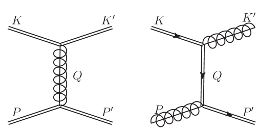
Figure 1: Typical diagrams contributing to ${2\leftrightarrow 2}$ processes at LO. Double lines represent hard or thermal particles, which have at least one momentum component of the order of the temperature or larger. Parallel double lines without arrows can be either gluons or quarks. When particle identities need to be specified, quarks are identified by the fermion flow arrow and gluons by the curly line. In all diagrams in the paper, time is understood to flow from left to right.

The ${1\leftrightarrow 2}$ rates describe the collinear radiation from the jet-like particles, which is induced by multiple soft scatterings with the background plasma, see Fig. 2. Although apparently suppressed by powers of $g$, multiple scatterings contribute at leading order under the provision that: (a) the momenta of the hard lines are nearly on shell and collinear to each other (i.e.  $\theta{\ \lower-1.2pt\vbox{\hbox{\hbox to0.0pt{$<$\hss}\lower 6.0pt\vbox{\hbox{$\sim$}}}}\ }g$, where $\theta$ is the emission angle), and (b) the momenta $K$ of the soft gluons are space-like $k^{+},k_{\perp}\sim gT$ and $k^{-}{\ \lower-1.2pt\vbox{\hbox{\hbox to0.0pt{$<$\hss}\lower 6.0pt\vbox{\hbox{$\sim$}}}}\ }g^{2}T$. A complete leading order treatment of collinear radiation must consistently resum these soft scatterings to account for the Landau-Pomeranchuk-Migdal (LPM) effect Baier:1994bd ; Baier:1996kr ; Zakharov:1996fv ; Zakharov:1997uu ; Arnold:2002ja .

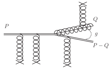
Figure 2: A typical diagram contributing to ${1\leftrightarrow 2}$ processes at LO. The single curly line is a soft gluon. The crosses represent the soft thermal scattering centers – see, for instance, ref. Arnold:2002ja .

In detail, the collision operator reads (dropping for brevity the spacetime dependence, which is local)

$$C_{a}^{2\leftrightarrow 2}[f]({\bm{p}}) = \frac{1}{4|{\bm{p}}|\nu_{a}}\sum_{bcd}\int_{{\bm{k}}{\bm{p}}^{\prime}{\bm{k}}^{\prime}}\left|{\cal M}^{ab}_{cd}({\bm{p}},{\bm{k}};{\bm{p}}^{\prime},{\bm{k}}^{\prime})\right|^{2}\>(2\pi)^{4}\,\delta^{(4)}(P+K-P^{\prime}-K^{\prime})$$ (2)

$$\hskip 65.04256pt{}\times\Bigl{\{}f^{a}({\bm{p}})\,f^{b}({\bm{k}})\,[1{\pm}f^{c}({\bm{p}}^{\prime})]\,[1{\pm}f^{d}({\bm{k}}^{\prime})]$$

$$\hskip 72.26999pt{}-f^{c}({\bm{p}}^{\prime})\,f^{d}({\bm{k}}^{\prime})\,[1{\pm}f^{a}({\bm{p}})]\,[1{\pm}f^{b}({\bm{k}})]\Bigr{\}}\,,$$

and

$$C_{a}^{1\leftrightarrow 2}[f]({\bm{p}}) = \frac{(2\pi)^{3}}{2|{\bm{p}}|^{2}\nu_{a}}\sum_{bc}\int_{0}^{\infty}dp^{\prime}\>dq^{\prime}\;\delta(|{\bm{p}}|-p^{\prime}-q^{\prime})\;\gamma^{a}_{bc}({\bm{p}};p^{\prime}\hat{\bm{p}},q^{\prime}\hat{\bm{p}})$$ (3)

$$\hskip 30.00005pt{}\times\Bigl{\{}f^{a}({\bm{p}})\,[1{\pm}f^{b}(p^{\prime}\hat{\bm{p}})]\,[1{\pm}f^{c}(q^{\prime}\hat{\bm{p}})]-f^{b}(p^{\prime}\hat{\bm{p}})f^{c}(q^{\prime}\hat{\bm{p}})\,[1{\pm}f^{a}({\bm{p}})]\Bigr{\}}$$

$$+ \frac{(2\pi)^{3}}{|{\bm{p}}|^{2}\nu_{a}}\sum_{bc}\int_{0}^{\infty}dq\>dp^{\prime}\;\delta(|{\bm{p}}|+q-p^{\prime})\;\gamma_{ab}^{c}(p^{\prime}\hat{\bm{p}};{\bm{p}},q\,\hat{\bm{p}})$$

$$\hskip 20.00003pt{}\times\Bigl{\{}f^{a}({\bm{p}})\,f^{b}(q\hat{\bm{p}})[1{\pm}f^{c}(p^{\prime}\hat{\bm{p}})]-f^{c}(p^{\prime}\hat{\bm{p}})\,[1{\pm}f^{a}({\bm{p}})][1{\pm}f^{b}(q\hat{\bm{p}})]\Bigr{\}},\quad$$

where the sum runs over the species $bc(d)$ in the scattering/splitting event, and the splitting kernel $\gamma^{a}_{bc}$ is defined in Eq. (5.1–5.4) of Ref. Arnold:2002zm , see also Eq. (45). We are also using the shorthand notation

$$\int_{\bm{k}}\ldots\equiv\int\frac{d^{3}k}{2k(2\pi)^{3}}\ldots$$ (4)

for the Lorentz-invariant integration. The matrix elements $\mathcal{M}$ and transverse-momentum integrated matrix elements $\gamma$ will be discussed in the following. $\nu^{a}=2d_{R}$ is the degeneracy of the particle $a$: two spin degrees of freedom and $d_{R}$ color degrees of freedom, where $d_{R}$ is the dimension of the representation of $a$. For quarks it is $d_{F}=N_{c}$, for gluons $d_{A}=N_{c}^{2}-1$.

The hard particles are very dilute, and therefore we only need to track the interactions of these modes with the thermal and soft constituents. This can be done by defining $\delta\!f$

$$f^{a}({\bm{p}},{\bm{x}},t)=n^{a}({\bm{p}},T({\bm{x}},t),{\bm{u}}({\bm{x}},t))+\delta\!f^{a}({\bm{p}},{\bm{x}},t),$$ (5)

and linearizing the Boltzmann equation in this quantity. Here $n$ is the (local) equilibrium distribution, written generally as a function of the local temperature $T$ and flow velocity ${\bm{u}}$. In the following we will work in the local rest frame where $n$ becomes the Fermi–Dirac distribution $n_{\scriptscriptstyle F}(p)$ or the Bose–Einstein distribution $n_{\scriptscriptstyle B}(p)$. Substituting Eq. (5) in the collision operator and dropping terms which are of order $e^{-p/T}$ yields

$$C_{a}^{2\leftrightarrow 2}[\delta\!f]({\bm{p}}) = \frac{1}{4|{\bm{p}}|\nu_{a}}\sum_{bcd}\int_{{\bm{k}}{\bm{p}}^{\prime}{\bm{k}}^{\prime}}\left|{\cal M}^{ab}_{cd}({\bm{p}},{\bm{k}};{\bm{p}}^{\prime},{\bm{k}}^{\prime})\right|^{2}\>(2\pi)^{4}\,\delta^{(4)}(P+K-P^{\prime}-K^{\prime})$$ (6)

$${}\times\Bigl{\{}\delta\!f^{a}({\bm{p}})\,n^{b}(k)\,[1{\pm}n^{c}(p^{\prime}){\pm}n^{d}(k^{\prime})]-\delta\!f^{c}({\bm{p}}^{\prime})\,n^{d}(k^{\prime})\,[1{\pm}n^{b}(k)]$$

$$\phantom{\times\Bigl{\{}}{}-n^{c}(p^{\prime})\,\delta\!f^{d}({\bm{k}}^{\prime})\,[1{\pm}n^{b}(k)]\Bigr{\}}\,,$$

and

$$C_{a}^{1\leftrightarrow 2}[\delta\!f]({\bm{p}}) = \frac{(2\pi)^{3}}{2|{\bm{p}}|^{2}\nu_{a}}\sum_{bc}\int_{0}^{\infty}dp^{\prime}\>dq^{\prime}\;\delta(|{\bm{p}}|-p^{\prime}-q^{\prime})\;\gamma^{a}_{bc}({\bm{p}};p^{\prime}\hat{\bm{p}},q^{\prime}\hat{\bm{p}})$$ (7)

$${}\times\Bigl{\{}\delta\!f^{a}({\bm{p}})\,[1{\pm}n^{b}(p^{\prime}){\pm}n^{c}(q^{\prime})]-[\delta\!f^{b}(p^{\prime}\hat{\bm{p}})n^{c}(q^{\prime})+n^{b}(p^{\prime})\delta\!f^{c}(k^{\prime}\hat{\bm{p}})]\Bigr{\}}$$

$$+ \frac{(2\pi)^{3}}{|{\bm{p}}|^{2}\nu_{a}}\sum_{bc}\int_{0}^{\infty}dq\>dp^{\prime}\;\delta(|{\bm{p}}|+q-p^{\prime})\;\gamma_{ab}^{c}(p^{\prime}\hat{\bm{p}};{\bm{p}},q\,\hat{\bm{p}})$$

$${}\times\Bigl{\{}\delta\!f^{a}({\bm{p}})\,n^{b}(q)-\delta\!f^{c}(p^{\prime}\hat{\bm{p}})[1{\pm}n^{b}(q)]\Bigr{\}}.\quad$$

These are to be used in a linearized Boltzmann equation for the hard components $\delta\!f^{a}({\bm{p}})$,

$$\left(\frac{\partial}{\partial t}+v_{\bm{x}}\cdot\bm{\nabla}_{x}\right)\delta\!f^{a}({\bm{p}},{\bm{x}},t)=-C_{a}^{\mathrm{LO}}[\delta\!f]=-C_{a}^{2\leftrightarrow 2}[\delta\!f]-C_{a}^{1\leftrightarrow 2}[\delta\!f]\,.$$ (8)

In the ${2\leftrightarrow 2}$ collision integrals, soft gluon and fermion exchanges must be screened to avoid logarithmic divergences. At leading order, the bare $t-$ and $u-$channel propagators may be replaced with their Hard Thermal Loop counterparts in the infrared to render the collision integrals finite. This procedure (which is detailed in Appendix A of Arnold:2003zc ) provides the leading weak-coupling description for soft exchanges, and is correct to order $g^{2}$ for hard exchanges. However, while this regularization prescription provides the correct leading order answer, it is not easily generalized to NLO. Further, the approach mixes different physics at different scales. In the next section we will re-examine the ${2\leftrightarrow 2}$ collision rates, incorporating soft $t,u-$channel exchanges into drag, diffusion, and conversion coefficients, which cleanly reflect the physics of the Debye sector. Then, in Sec. 4, we will compute these transport parameters at NLO.

3 A reorganization of leading order: large-angle scattering, drag and diffusion, and conversions

The leading order picture we have just described, with distinct ${1\leftrightarrow 2}$ collinear processes and ${2\leftrightarrow 2}$ processes dressed with HTLs for IR finiteness, starts to be ill-defined at NLO. Consider the soft limit of the ${2\leftrightarrow 2}$ processes. In the case of a soft gluon exchange, as shown in Fig. 3,

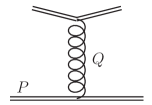
Figure 3: The soft limit of a $t-$ or $u-$channel gluon exchange diagram. $P$ is the hard momentum and $Q$ is the soft gluon momentum.

we obtain a process which changes the hard four-momentum $P$ by a small amount $Q\sim gT$, without changing the particle identity. We call such a process a diffusion process, since, as described in Sec. 3.2, they can be treated in a diffusion approximation.

In the case of a soft quark exchange, as shown in Fig. 4, one obtains an identity-changing process.

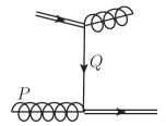
Figure 4: The soft limit of a $t-$ or $u-$channel quark exchange diagram. $P$ is the hard momentum and $Q$ is the soft quark momentum.

Here a hard gluon with momentum $P$ is turned into a quark with an almost equivalent momentum, up to $O(gT)$. We then call these processes conversion processes, and we will deal with them in a different way, inspired by the NLO thermal photon rate Ghiglieri:2013gia .

Now consider a collinear ${1\leftrightarrow 2}$ process in the limit where one of the hard/thermal legs becomes soft, as shown in Fig. 5.

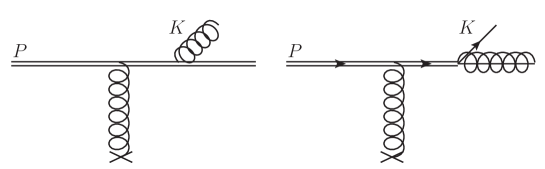
Figure 5: The soft-$K$ limits of a ${1\leftrightarrow 2}$ process. The diagram on the left amounts to a diffusion process at NLO, whereas the diagram on the right amounts to a conversion process.

In the first graph, the soft gluon emission contributes to the (longitudinal) diffusion of the hard particle. Similarly the soft quark emission contributes to the hard quark conversion rate. At NLO we will then need to subtract these limits from the collinear ${1\leftrightarrow 2}$ region and treat them as part of the diffusion or conversion processes respectively.

To summarize, at leading order we can rewrite the right-hand side of Eq. (8) as

$$-C_{a}^{\mathrm{LO}}[\delta\!f]=-C_{a}^{\mathrm{large}}[\delta\!f]-C_{a}^{\mathrm{coll}}[\delta\!f]-C_{a}^{\mathrm{diff}}[\delta\!f]-C_{a}^{\mathrm{conv}}[\delta\!f].$$ (9)

Here $C^{\mathrm{large}}$ is the ${2\leftrightarrow 2}$ collision operator restricted to large momentum transfers, $Q\gg gT$. Defining this scattering rate requires regularization procedure, which we describe in the next section, Sec. 3.1. $C^{\mathrm{diff}}$ notates a diffusion approximation to the collision integral for small momentum transfer, $Q\sim gT$. This is discussed in Sec. 3.2, where the LO longitudinal and transverse diffusion coefficients are extracted from the screened $2\leftrightarrow 2$ rates. Similarly, $C^{\mathrm{conv}}$ notates the conversion processes, and the appropriate LO conversion coefficients are found in Sec. 3.3. The precise value of these diffusion and conversion coefficients depends on the regulator, but the dependence on the regulator cancels to leading order when $C^{\rm large},C^{\rm diff}$, and $C^{\rm conv}$ are taken together in Eq. (9). Finally, $C^{\mathrm{coll}}$ consists of the collinear ${1\leftrightarrow 2}$ rates $C^{{1\leftrightarrow 2}}$ after excluding (or subtracting) the diffusion and conversion-like emissions shown in Fig. 5. These soft emissions (which were originally included in the $C^{{1\leftrightarrow 2}}$ rates) are limited in phase space to $K\sim gT$, and their exclusion constitutes an $\mathcal{O}(g)$ correction. Thus, at leading order $C_{a}^{\mathrm{coll}}[\delta\!f]=C^{{1\leftrightarrow 2}}[\delta\!f]$. We therefore will present the explicit form of $C^{\mathrm{coll}}$ only when we describe its NLO corrections in Sec. 5.

3.1 Large-angle scattering

In this section, we describe the integration of the $2\leftrightarrow 2$ matrix elements with large momentum transfer, $Q\gg gT$, which enters in the leading order collision kernel $C_{a}^{\mathrm{large}}$ in Eq. (9). This is completely straightforward, but integrals of the bare matrix elements must be regulated with some scheme. The cutoff regulator chosen in this section conveniently matches with the calculations of the diffusion and conversion coefficients in Sec. 3.2 and 3.3.

In more detail, to evaluate $C_{a}^{\mathrm{large}}[\delta\!f]$, one needs integrate the matrix elements listed in Table 1, i.e. the standard, leading-order QCD matrix elements, summed over all color and spin indices, with the Mandelstam variables $s=-(P+K)^{2}$, $t=-(P-P^{\prime})^{2}$ and $u=-(P-K^{\prime})^{2}$. To regulate gluon and fermion exchanges in the $t$ and $u$ channels we use the integration technology of Ref. Arnold:2003zc , which treats each channel differently.

$ab\leftrightarrow cd$	$\qquad\left|{\cal M}^{ab}_{cd}\right|^{2}/g^{4}$
$\begin{array}[]{c}q_{1}q_{2}\leftrightarrow q_{1}q_{2}\,,\\ q_{1}\bar{q}_{2}\leftrightarrow q_{1}\bar{q}_{2}\,,\\ \bar{q}_{1}q_{2}\leftrightarrow\bar{q}_{1}q_{2}\,,\\ \bar{q}_{1}\bar{q}_{2}\leftrightarrow\bar{q}_{1}\bar{q}_{2}\end{array}$	$\displaystyle 8\,\frac{d_{F}^{2}\,C_{F}^{2}}{d_{A}}\left(\frac{s^{2}+u^{2}}{\underline{t^{2}}}\right)$
$\begin{array}[]{c}q_{1}q_{1}\leftrightarrow q_{1}q_{1}\,,\\ \bar{q}_{1}\bar{q}_{1}\leftrightarrow\bar{q}_{1}\bar{q}_{1}\end{array}$	$\displaystyle 8\,\frac{d_{F}^{2}\,C_{F}^{2}}{d_{A}}\left(\frac{s^{2}+u^{2}}{\underline{t^{2}}}+\frac{s^{2}+t^{2}}{\underline{u^{2}}}\right)+16\,d_{F}\,C_{F}\left(C_{F}{-}\frac{C_{A}}{2}\right)\frac{s^{2}}{tu}$
$q_{1}\bar{q}_{1}\leftrightarrow q_{1}\bar{q}_{1}$	$\displaystyle 8\,\frac{d_{F}^{2}\,C_{F}^{2}}{d_{A}}\left(\frac{s^{2}+u^{2}}{\underline{t^{2}}}+\frac{t^{2}+u^{2}}{s^{2}}\right)+16\,d_{F}\,C_{F}\left(C_{F}{-}\frac{C_{A}}{2}\right)\frac{u^{2}}{st}$
$q_{1}\bar{q}_{1}\leftrightarrow q_{2}\bar{q}_{2}$	$\displaystyle 8\,\frac{d_{F}^{2}\,C_{F}^{2}}{d_{A}}\left(\frac{t^{2}+u^{2}}{s^{2}}\right)$
$q_{1}\bar{q}_{1}\leftrightarrow g\,g$	$\displaystyle 8\,d_{F}\,C_{F}^{2}\left(\frac{u}{\underline{\underline{t}}}+\frac{t}{\underline{\underline{u}}}\right)-8\,d_{F}\,C_{F}\,C_{A}\left(\frac{t^{2}+u^{2}}{s^{2}}\right)$
$\begin{array}[]{c}q_{1}\,g\leftrightarrow q_{1}\,g\,,\\ \bar{q}_{1}\,g\leftrightarrow\bar{q}_{1}\,g\end{array}$	$\displaystyle-8\,d_{F}\,C_{F}^{2}\left(\frac{u}{s}+\frac{s}{\underline{\underline{u}}}\right)+8\,d_{F}\,C_{F}\,C_{A}\left(\frac{s^{2}+u^{2}}{\underline{t^{2}}}\right)$
$g\,g\leftrightarrow g\,g$	$\displaystyle 16\,d_{A}\,C_{A}^{2}\left(3-\frac{su}{\underline{t^{2}}}-\frac{st}{\underline{u^{2}}}-\frac{tu}{s^{2}}\right)$

Table 1: Squares of vacuum matrix elements for $2\leftrightarrow 2$ particle processes in QCD-like theories, summed over all spins and colors. $q_{1}$ and $q_{2}$ represent fermions of distinct flavors, $\bar{q}_{1}$ and $\bar{q}_{2}$ are the associated antifermions, and $g$ represents a gluon.

Singly-underlined matrix elements come from gluon exchange diagrams, and are those that, in the soft limit, give rise to gluonic IR divergences, corresponding to diffusion processes. Similarly, doubly-underlined matrix elements come from fermion-exchange diagrams and give rise, in the same limit, to conversion processes. To illustrate the regularization scheme, let us consider the contribution from the scattering of different quark species $q_{1}q_{2}\leftrightarrow q_{1}q_{2}$, which is given by the square of a single $t$-channel diagram. The $q_{1}q_{2}\leftrightarrow q_{1}q_{2}$ contribution to $C_{q_{1}}^{\mathrm{large}}[\delta\!f]$ reads

$$C_{q_{1}}^{\mathrm{large}}[\delta\!f] \supset \frac{g^{4}}{(2\pi)^{3}}\frac{C_{F}}{16p^{2}}\int_{-\infty}^{+\infty}d\omega\int_{0}^{2p-\omega}dq\int_{(q-\omega)/2}^{\infty}dk\theta(q-|\omega|)\int_{0}^{2\pi}\frac{d\phi}{2\pi}\frac{s^{2}+u^{2}}{t^{2}}$$ (10)

$$\times\Bigl{\{}\delta\!f^{q_{1}}(p)\,n_{\scriptscriptstyle F}(k)\,[1-n_{\scriptscriptstyle F}(p-\omega)-n_{\scriptscriptstyle F}(k+\omega)]$$

$$\hskip 14.22636pt-\big{[}\delta\!f^{q_{1}}(p-\omega)\,n_{\scriptscriptstyle F}(k+\omega)+\delta\!f^{q_{2}}(k+\omega)\,n_{\scriptscriptstyle F}(p-\omega)\big{]}\,[1-n_{\scriptscriptstyle F}(k)]\Bigr{\}},$$

where the techniques of Arnold:2003zc have been followed, by (i) eliminating one of the three integration variables in Eq. (6) with the momentum-conserving $\delta$-function, (ii) shifting one of the remaining ones to ${\bm{q}}\equiv{\bm{p}}-{\bm{p}}^{\prime}={\bm{k}}^{\prime}-{\bm{k}}$, (iii) introducing $\omega\equiv p-p^{\prime}=k^{\prime}-k$, and (iv) performing the angular integrations. The remaining angle $\phi$ represents the azimuthal angle between the $({\bm{p}},{\bm{q}})$ plane and the $({\bm{k}},{\bm{q}})$ plane.

The Mandelstam variables become

$$s=-\frac{t}{2q^{2}}\left[(p+p^{\prime})(k+k^{\prime})+q^{2}-\cos(\phi)\sqrt{(4pp^{\prime}+t)(4kk^{\prime}+t)}\right],\quad t=\omega^{2}-q^{2},$$ (11)

and $p^{{}^{\prime}0}=p^{\prime}$, $k^{{}^{\prime}0}=k^{\prime}$ imply

$$\omega-\hat{{\bm{p}}}\cdot{\bm{q}}=\frac{\omega^{2}-q^{2}}{2p},\qquad\omega-\hat{{\bm{k}}}\cdot{\bm{q}}=-\frac{\omega^{2}-q^{2}}{2k}.$$ (12)

It is then easy to see how the unscreened logarithmic divergences show up for $\omega,q\sim gT\ll k,p$. To separate off the divergent region (which will match with the diffusion operator $C^{\mathrm{diff}}[\delta\!f]$ described in Sec. 3.2), we change integration variables from $\omega,q$ to $\omega,\tilde{q}_{\perp}$ with $\tilde{q}_{\perp}\equiv\sqrt{-t}=\sqrt{q^{2}-\omega^{2}}$. We can then place an IR cutoff $T\gg\mu_{\tilde{q}_{\perp}}\gg gT$ on $\tilde{q}_{\perp}$, leaving

$$C_{q_{1}}^{\mathrm{large}}[\delta\!f]\supset \frac{g^{4}}{(2\pi)^{3}}\frac{C_{F}}{16p^{2}}\int_{-\infty}^{p}d\omega\int_{\mu_{\tilde{q}_{\perp}}}^{\sqrt{4p(p-\omega)}}d\tilde{q}_{\perp}\frac{\tilde{q}_{\perp}}{q}\int_{(q-\omega)/2}^{\infty}dk\int_{0}^{2\pi}\frac{d\phi}{2\pi}\frac{s^{2}+u^{2}}{t^{2}}$$

$$\times\Bigl{\{}\delta\!f^{q_{1}}(p)\,n_{\scriptscriptstyle F}(k)\,[1-n_{\scriptscriptstyle F}(p-\omega)-n_{\scriptscriptstyle F}(k+\omega)]$$

$$\hskip 14.22636pt-\big{[}\delta\!f^{q_{1}}(p-\omega)\,n_{\scriptscriptstyle F}(k+\omega)+\delta\!f^{q_{2}}(k+\omega)\,n_{\scriptscriptstyle F}(p-\omega)\big{]}\,[1-n_{\scriptscriptstyle F}(k)]\Bigr{\}}.$$ (13)

Eq. (13) implicitly depends on the cutoff $\mu_{\tilde{q}_{\perp}}$. For small $\tilde{q}_{\perp}$ the dominant $\omega$ region is also small, and the fermion distribution can be approximated as, $n_{\scriptscriptstyle F}(p-\omega)\simeq n_{\scriptscriptstyle F}(p)$.

In the small $\tilde{q}_{\perp}$ regime, the scattering rate integrated over $\omega$ turns out to take a very simple form in terms of this variable, which is the real motivation for its use. In addition, the physical interpretation of $\tilde{q}_{\perp}$ in this regime is the transverse momentum transferred to the ${\bm{p}}$ particle; specifically, in terms of the $P$-defined light-cone coordinates, we have for soft $Q$

$$\tilde{q}_{\perp}^{2} = q_{\perp}^{2}\left(1+\frac{q^{+}}{p}+\mathcal{O}\left(\frac{g^{2}T^{2}}{p^{2}}\right)\right),\qquad\omega=q^{+}-\frac{q_{\perp}^{2}}{4p}+\mathcal{O}\left(\frac{g^{2}T^{2}}{p^{2}}\right),$$

$$q^{z} = q^{+}+\frac{q_{\perp}^{2}}{4p}+\mathcal{O}\left(\frac{g^{2}T^{2}}{p^{2}}\right)=\omega+\frac{\tilde{q}_{\perp}^{2}}{2p}+\mathcal{O}\left(\frac{g^{2}T^{2}}{p^{2}}\right).$$ (14)

Finally, let us analyze the power counting. Above the cutoff, when angles are large, the contribution to the collision operator is of order $g^{4}T$, up to powers of $T/E$. When $q,\omega\sim gT$, the $\phi$-averaged matrix element is proportional to $p^{2}k^{2}/q^{4}\sim 1/g^{4}$, up to corrections, which combined with $dqd\omega\sim g^{2}$ and with another $g^{2}$ coming from the expansion of the curly brackets for small $Q$ make the singly-underlined exchanges contribute to LO in the soft region, with a $\ln(g)$ enhancement. The same happens (without cancellations) for the doubly-underlined matrix elements. Non-underlined matrix elements with $st$ or $tu$ at the denominator are suppressed by a further power of $g^{2}$ in the soft region. Since the integration is finite, $\mu_{\tilde{q}_{\perp}}$ can be pushed to zero there for simplicity. Singly underlined matrix elements with a $u^{2}$ at the denominator present the same divergences; they can be dealt with by swapping the $k^{\prime}$ and $p^{\prime}$ labels and using the same parameterization. Matrix elements with $s^{2}$ at the denominator are not sensitive to the soft region; hence, at leading order, they can be integrated without cutoffs as well.

Fermion exchanges, and in particular the log-divergent doubly-underlined $t$- or $u$-channel exchanges, can be treated with the same techniques and $\mu_{\tilde{q}_{\perp}}$ cutoffs. For illustration, the $t$-channel quark exchange contribution to $q_{1}\bar{q}_{1}\leftrightarrow gg$ scattering is

$$C_{q_{1}}^{\mathrm{large}}[\delta\!f]\supset \frac{g^{4}}{(2\pi)^{3}}\frac{C_{F}^{2}}{8p^{2}}\int_{-\infty}^{p}d\omega\int_{\mu_{\tilde{q}_{\perp}}}^{\sqrt{4p(p-\omega)}}d\tilde{q}_{\perp}\frac{\tilde{q}_{\perp}}{q}\int_{(q-\omega)/2}^{\infty}dk\int_{0}^{2\pi}\frac{d\phi}{2\pi}\frac{u}{t}$$

$$\times\Bigl{\{}\delta\!f^{q_{1}}(p)\,n_{\scriptscriptstyle F}(k)\,[1+n_{\scriptscriptstyle B}(p-\omega)+n_{\scriptscriptstyle B}(k+\omega)]$$

$$\hskip 14.22636pt-\big{[}\delta\!f^{g}(p-\omega)\,n_{\scriptscriptstyle B}(k+\omega)+\delta\!f^{g}(k+\omega)\,n_{\scriptscriptstyle B}(p-\omega)\big{]}\,[1-n_{\scriptscriptstyle F}(k)]\Bigr{\}}.$$ (15)

The cancellations of the leading IR behavior in the gluon exchanges, as well as the matching to the diffusion and conversion processes will be dealt with in the next sections and in App. D.

3.2 Diffusion processes

In this section we will describe the diffusion collision kernel, $C^{\mathrm{diff}}$, in greater detail. The cumulative effect of a large number of small momentum-transfer collisions that preserve the identity of the hard particles can be summarized by a Fokker-Plank equation Svetitsky:1987gq ; Moore:2004tg

$$C_{a}^{\mathrm{diff}}[\delta\!f]\equiv-\frac{\partial}{\partial p^{i}}\bigg{[}\eta_{\scriptscriptstyle D}(p)p^{i}\delta\!f^{a}({\bm{p}})\bigg{]}-\frac{1}{2}\frac{\partial^{2}}{\partial p^{i}\partial p^{j}}\left[\left(\hat{p}^{i}\hat{p}^{j}\hat{q}_{\scriptscriptstyle L}(p)+\frac{1}{2}(\delta^{ij}-\hat{p}^{i}\hat{p}^{j})\hat{q}(p)\right)\delta\!f^{a}({\bm{p}})\right].$$ (16)

App. D directly shows how the diffusion operator arises at leading order from the screened $2\leftrightarrow 2$ collisions kernel, Eq. (2). There are three coefficients that enter in this effective description: $\hat{q}$ is the standard transverse momentum broadening, $\hat{q}_{\scriptscriptstyle L}$ is the longitudinal momentum broadening and $\eta_{\scriptscriptstyle D}$ is the drag coefficient. They are defined as

$$\eta_{\scriptscriptstyle D}(p)=-\frac{1}{p_{\scriptscriptstyle L}}\frac{dp_{\scriptscriptstyle L}}{dt},\qquad\hat{q}(p)\equiv\frac{d}{dt}\left\langle(\Delta p_{\perp})^{2}\right\rangle,\qquad\hat{q}_{\scriptscriptstyle L}(p)\equiv\frac{d}{dt}\left\langle(\Delta p_{\scriptscriptstyle L})^{2}\right\rangle,$$ (17)

where $p_{\scriptscriptstyle L}$ and ${\bm{p}}_{\perp}$ are the longitudinal and transverse components relative to the large momentum ${\bm{p}}$.

These coefficients can be determined through the interaction rates Svetitsky:1987gq ; Braaten:1991jj ; Moore:2004tg , i.e.

$$\frac{dp_{\scriptscriptstyle L}}{dt} = -\int dq^{z}\,q^{z}\,\frac{d\Gamma({\bm{p}},{\bm{p}}-{\bm{q}})}{dq^{z}},$$ (18)

$$\hat{q}_{\scriptscriptstyle L}(p) = \int dq^{z}\,(q^{z})^{2}\,\frac{d\Gamma({\bm{p}},{\bm{p}}+{\bm{q}})}{dq^{z}},$$ (19)

$$\hat{q}(p) = \int d^{2}q_{\perp}\,q_{\perp}^{2}\,\frac{d\Gamma({\bm{p}},{\bm{p}}+{\bm{q}})}{d^{2}q_{\perp}},$$ (20)

where $\Gamma({\bm{p}},{\bm{p}}\pm{\bm{q}})$ is the transition rate from initial hard momentum ${\bm{p}}$ to final hard momentum ${\bm{p}}\pm{\bm{q}}$, with ${\bm{q}}$ soft. A regulator which cuts off the $Q$ integrations is implicit, and the values of these coefficients will in general depend on the chosen scheme. Rather than determining $\Gamma({\bm{p}},{\bm{p}}\pm{\bm{q}})$ and evaluating the integrals in these equations directly, it is convenient (especially at NLO) to use field-theoretical definitions for the coefficients in Eq. (16)

The transverse scattering rate $d\Gamma/d^{2}q_{\perp}$ at large momentum is traditionally parameterized by ${\mathcal{C}}(q_{\perp})$

$$\lim_{p\to\infty}\frac{d\Gamma({\bm{p}},{\bm{p}}+{\bm{q}}_{\perp})}{d^{2}q_{\perp}}=\frac{{\mathcal{C}}(q_{\perp})}{(2\pi)^{2}}.$$ (21)

In $p\to\infty$ limit the hard particle’s behavior eikonalizes, and ${\mathcal{C}}(q_{\perp})$ can be defined in terms of a specific Wilson loop CaronHuot:2008ni ; Benzke:2012sz in the $(x^{+},x_{\perp})$ plane (for propagation in the positive $z$ direction). Using this Wilson loop definition, ${\mathcal{C}}(q_{\perp})$ and $\hat{q}$ have been evaluated at leading Aurenche:2002pd and next-to-leading orders CaronHuot:2008ni . In particular, at leading order the result is

$${\mathcal{C}}_{R}(q_{\perp})=g^{2}C_{R}\int\frac{dq^{0}dq_{z}}{(2\pi)^{2}}2\pi\delta(q^{0}-q_{z})G_{rr}^{--}(Q)=g^{2}C_{R}T\frac{m_{\scriptscriptstyle D}^{2}}{q_{\perp}^{2}(q_{\perp}^{2}{+}m_{\scriptscriptstyle D}^{2})}\,,$$ (22)

where $R$ labels the representation of the source and $m_{\scriptscriptstyle D}^{2}=g^{2}T^{2}(N_{c}/3+N_{f}/6)$ is the leading order Debye mass. $\hat{q}$ then reads at LO

$$\hat{q}=\int\frac{d^{2}q_{\perp}}{(2\pi)^{2}}q_{\perp}^{2}{\mathcal{C}}_{R}(q_{\perp})=g^{2}C_{R}T\int\frac{d^{2}q_{\perp}}{(2\pi)^{2}}\frac{m_{\scriptscriptstyle D}^{2}}{(q_{\perp}^{2}{+}m_{\scriptscriptstyle D}^{2})}=\frac{g^{2}C_{R}Tm_{\scriptscriptstyle D}^{2}}{2\pi}\ln\frac{\mu_{\tilde{q}_{\perp}}}{m_{\scriptscriptstyle D}}\,,$$ (23)

where, since we are in the $p\to\infty$ limit, $\tilde{q}_{\perp}=q_{\perp}$ and we have used $\mu_{\tilde{q}_{\perp}}$ as UV regulator.

What makes the Wilson loop definition particularly attractive is that it can be evaluated CaronHuot:2008ni using the (much simpler) Euclidean, dimensionally-reduced Electrostatic QCD (EQCD) Braaten:1994na ; Braaten:1995cm ; Braaten:1995jr ; Kajantie:1995dw ; Kajantie:1997tt . This made the NLO computation possible CaronHuot:2008ni , and opened the door to recent non-perturbative lattice measurements Laine:2013lia ; Panero:2013pla . These formal definitions, as well as those for related light-front operators, are summarized in App. B of Ghiglieri:2013gia and reviewed in Ghiglieri:2015zma .

These techniques and results, like most eikonal expansions, are based on a large momentum expansion, $p\gg T$ or $gT$. In App. D we study the finite-$p$ corrections, showing that $T/p$ suppressed corrections are really corrections in $gT/p$; and the first correction involves vanishing odd integrands, so the first nonzero corrections from this expansion are $\mathcal{O}(g^{2})$ even for $p\sim T$, and are therefore irrelevant at the level of precision we are seeking here. Therefore we can use the leading (and later, subleading) order calculations in the strict Wilson-line limit which we have just discussed.

To fully specify the diffusion operator $C^{\mathrm{diff}}$ in Eq. (16) we also need to evaluate the longitudinal diffusion and drag coefficients, $\hat{q}_{\scriptscriptstyle L}$ and $\eta_{\scriptscriptstyle D}$. To this end, we will first compute the diffusion coefficient $\hat{q}_{\scriptscriptstyle L}$ and then use fluctuation-dissipation relations to determine the drag (see below). At the practical level, we introduce a Wilson-line based definition for $\hat{q}_{\scriptscriptstyle L}$ in the $p\to\infty$ limit, or equivalently at leading order in $T/p$. In App. C we will give a more formal justification for our definition, whereas in App. D we show that, as in the previous paragraph, finite-momentum corrections start at $\mathcal{O}(g^{2})$, and are thus irrelevant to current accuracy.

Intuitively, longitudinal momentum diffusion occurs because the longitudinal force along the particle’s trajectory has a nonzero correlator. Experience with $\hat{q}$ and heavy quark diffusion CasalderreySolana:2006rq ; Gubser:2006nz suggests that $\hat{q}_{\scriptscriptstyle L}$ should be given by a lightlike longitudinal force-force correlator. The force is determined by the electric field in the direction of propagation, which motivates the following operator definition for $\hat{q}_{\scriptscriptstyle L}$ in the large momentum limit:

$$\hat{q}_{\scriptscriptstyle L} = \frac{g^{2}}{d_{R}}\int_{-\infty}^{+\infty}dx^{+}\,\mathrm{Tr}\left\langle U_{R}(-\infty,0,0_{\perp};x^{+},0,0_{\perp})\bar{v}_{\mu}v_{\nu}F^{\mu\nu}(x^{+},0,0_{\perp})\right.$$ (24)

$$\hskip 85.35826pt\left.U_{R}(x^{+},0,0_{\perp};0,0,0_{\perp})F^{\rho\sigma}(0)U_{R}(0;-\infty,0,0_{\perp})\bar{v}_{\rho}v_{\sigma}\right\rangle.$$

Here $v\equiv(1,0,0,1)$ and $\bar{v}\equiv(1/2,0,0,-1/2)$ are null vectors that are chosen to maintain our light-cone conventions (i.e. $p^{+}\equiv-\bar{v}\cdot P$, $p^{-}\equiv-v\cdot P$), and $F^{\mu\nu}\bar{v}_{\mu}v_{\nu}=F^{+-}=E^{z}$ is the electric field along the propagation direction. We are using a matrix notation, so that $F^{\mu\nu}=F^{\mu\nu\,a}T^{a}_{R}$, and $U_{R}$ is a straight Wilson line in the representation $R$ of the source

$$U_{R}(Y;X)=P\exp\left(-ig\int_{0}^{1}ds\,(Y-X)\cdot A_{R}(s(Y-X)+X)\right).$$ (25)

Gauge fields and matrices in the Wilson lines are both to be understood as path ordered. Eq. (24) comes from the eikonal approximation, i.e. the replacement of the highly energetic particle with momentum ${\bm{p}}$ with a Wilson line in the appropriate representation along its classical trajectory. We also note that this definition of $\hat{q}_{\scriptscriptstyle L}$ has the correct “amplitude times conjugate amplitude” structure required to enter in a rate.

We now evaluate Eq. (24) at LO: we simply contract the two $F$ fields, obtaining a forward Wightman correlator, i.e. the diagram shown in Fig. 6,

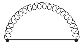
Figure 6: The leading-order soft contribution to $\hat{q}_{\scriptscriptstyle L}$. The Wilson lines before and after the two black dots, which represent the $F^{+-}$ vertices, cancel at leading order, whereas the one between the two dots always turns into an adjoint line, which we have represented as a double line. The curly line is a soft HTL gluon.

which reads

$$\hat{q}_{\scriptscriptstyle L}=g^{2}C_{R}\int_{-\infty}^{+\infty}dx^{+}\int\frac{d^{4}Q}{(2\pi)^{4}}e^{-iq^{-}x^{+}}(q^{+})^{2}G^{--\,>}(Q),$$ (26)

where $G^{>}(Q)$ is the HTL-resummed forward propagator and the integral is understood to run over soft momenta only. The $x^{+}$ integration sets $q^{-}$ to zero and, as we show in App. D, brings this expression into agreement with the one obtained from the rate-based definition in Eq. (19). Note that only the even-in-$q^{+}$ part of $G^{>}(q^{+},q^{-}=0,q_{\perp})$ contributes to the integral. Then, using the fluctuation-dissipation theorem, $G^{>}(Q)=(1+n_{B}(q^{0}))\rho(Q)$ with $\rho(Q)=G_{R}(Q)-G_{A}(Q)$, we expand for small $q^{0}=q^{+}\sim gT$ to find

$$\hat{q}_{\scriptscriptstyle L}=g^{2}C_{R}\int\frac{dq^{+}d^{2}q_{\perp}}{(2\pi)^{3}}Tq^{+}(G^{--}_{R}(q^{+},q_{\perp})-G^{--}_{A}(q^{+},q_{\perp})),$$ (27)

up to an $\mathcal{O}(g^{2})$ correction. Numerical integration is straightforward, using the HTL propagators given in App. B. Beyond leading order, however, one would be plagued with intricate multi-dimensional numerical integrals. However, as we anticipated in the introduction, we can perform the $q^{+}$ integration (and similar ones elsewhere) by resorting to the analyticity sum rule techniques developed in CaronHuot:2008ni ; Ghiglieri:2013gia . Since retarded (advanced) two-point functions are analytic in the upper (lower) half-plane in any time-like or light-like variable, we can deform the integration contours away from the real axis onto $\mathcal{C}_{R}$ ($|q^{+}|\gg gT$, $\mathrm{Im}\,q^{+}>0$) and $\mathcal{C}_{A}$ ($|q^{+}|\gg gT$, $\mathrm{Im}\,q^{+}<0$), as depicted in Fig. 7.

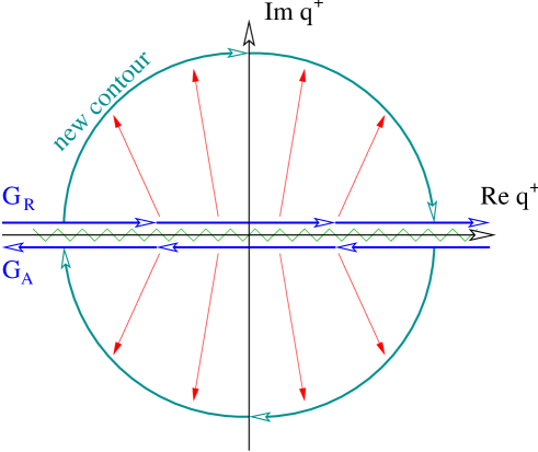
Figure 7: Integration contour in the complex $q^{+}$ integration, and the deformation we use to render $q^{+}\gg gT$. $G_{R}$ runs above the real axis and $G_{A}$ below.

Along the arcs the longitudinal and transverse propagators simplify greatly, i.e.

$$G^{--}_{R}(P)\to\frac{i}{(q^{+})^{2}}\left(1+\frac{q^{-}}{q^{+}}\right)\frac{2q^{+}q^{-}-M_{\infty}^{2}}{2q^{+}q^{-}-q_{\perp}^{2}-M_{\infty}^{2}}\Big{|}_{\mathcal{C}_{R}},$$ (28)

where $M_{\infty}^{2}\equiv m_{\scriptscriptstyle D}^{2}/2$ is the gluon asymptotic thermal mass. The end result is then

$$\hat{q}_{\scriptscriptstyle L}=g^{2}C_{R}T\int\frac{d^{2}q_{\perp}}{(2\pi)^{2}}\frac{M_{\infty}^{2}}{q_{\perp}^{2}+M_{\infty}^{2}}=\frac{g^{2}C_{R}T}{2\pi}M_{\infty}^{2}\ln\frac{\mu_{\tilde{q}_{\perp}}}{M_{\infty}},$$ (29)

where contributions smaller than $1/q^{+}$ in Eq. (28) are not needed, as they would only give rise to power-law terms in the cutoff on $q^{+}$ which would then cancel against contributions from larger scales. As in the $\hat{q}$ case, we have used $\mu_{\tilde{q}_{\perp}}$ as a transverse regulator, since the $(q^{+},q_{\perp})$ and $(\omega,\tilde{q}_{\perp})$ coordinates differ by $\mathcal{O}(g^{2})$ (all $\mathcal{O}(g)$ corrections vanish under integration).

The sum rule we have just obtained is the bosonic equivalent of the one presented in Ghiglieri:2013gia . Let us remark that the longitudinal and transverse contributions to $G_{R}^{--}(Q)$ contain poles at $q^{+}=q^{-}/2\pm iq_{\perp}$ ($q^{2}=0$), which, being on both sides of the complex plane, appear to violate analyticity. However their residue cancels in the sum of longitudinal and transverse components. As observed in CaronHuot:2008ni , they are artifacts of the decomposition into Lorentz-variant longitudinal and transverse modes and their contribution has to vanish in all gauge-invariant quantities.

We also remark that the same result (29) has been obtained in a different way in Peigne:2007sd for energy loss, which is related by an Einstein relation. As shown there, once the difference in regularization between $q_{\perp}<\mu_{\tilde{q}_{\perp}}$ and $q<\mu_{q}$ is taken into account, Eq. (29) agrees with the numerical results of Braaten and Thoma Braaten:1991jj for $v\to 1$.

Having determined $\hat{q}_{\scriptscriptstyle L}$, the drag coefficient $\eta_{\scriptscriptstyle D}(p)$ is constrained by the requirements that the Fokker-Planck description be equivalent to the Boltzmann one and that interactions with the medium tend to drive the hard excitations towards equilibrium Arnold:1999uza ; Arnold:1999va ; Moore:2004tg . Since we have taken a classical particle approximation for the hard particles, the equilibrium form is $\delta\!f({\bm{p}})\propto\exp(-p/T)$. The drag (in a given regularization scheme) is determined from $\hat{q}_{\scriptscriptstyle L}(p)$ and $\hat{q}(p)$ by adjusting the value of $\eta_{\scriptscriptstyle D}(p)$ so that Eq. (16) approaches equilibrium, i.e. its right-hand side vanishes for $\delta\!f({\bm{p}})\propto\exp(-p/T)$. Since $\hat{q}$ and $\hat{q}_{\scriptscriptstyle L}$ are $p$-independent up to $\mathcal{O}(g^{2})$, the equilibration condition yields to following relation:

$$\eta_{\scriptscriptstyle D}(p)=\frac{\hat{q}_{\scriptscriptstyle L}}{2Tp}+\frac{1}{2p^{2}}(\hat{q}-2\hat{q}_{\scriptscriptstyle L}).$$ (30)

The consistency of this condition is verified by direct computation of $\eta_{\scriptscriptstyle D}(p)$ and $\hat{q}_{\scriptscriptstyle L}$ at leading order in App. D. Inserting this relation between the coefficients into the diffusion equation, Eq. (16), we find

$$C_{a}^{\mathrm{diff}}[\delta\!f]=-\left[\frac{\delta\!f({\bm{p}})}{Tp}+\frac{2T+p}{2pT}\frac{d\delta\!f({\bm{p}})}{dp^{z}}+\frac{1}{2}\frac{d^{2}\delta\!f({\bm{p}})}{d(p^{z})^{2}}\right]\hat{q}_{\scriptscriptstyle L}-\left[-\frac{1}{2p}\frac{d\delta\!f({\bm{p}})}{dp^{z}}+\frac{1}{4}\nabla^{2}_{p_{\perp}}\delta\!f({\bm{p}})\right]\hat{q},$$ (31)

which is our final form for the diffusion operator.

We end by making a few remarks about the equilibrium condition and $\eta_{\scriptscriptstyle D}$. The first term in Eq. (30) comes from the simple Einstein relation that arises in the infinite momentum limit, i.e. $\hat{q}_{\scriptscriptstyle L}=-2Tdp_{\scriptscriptstyle L}/dt+\mathcal{O}(1/p)$. The relative $\mathcal{O}(1/p)$ terms can then be obtained by imposing equilibration on Eq. (16). In App. D we will show how, at leading order, those $1/p$ terms can be determined explicitly, how the diffusion picture matches exactly with $C^{\mathrm{large}}[\delta\!f]$ at large $Q$ and how different cutoff schemes can be implemented. It is also worth stressing that the $1/p$ terms to Eq. (30) and equivalently to $\eta_{\scriptscriptstyle D}$ do not come from a $T/p$ expansion, but only from the $g\ll 1$ expansion. Up to relative $\mathcal{O}(g^{2})$, there are no $1/p^{2}$ terms. Finally we remark that, in the simpler case where $\delta\!f$ is a function of $p$ rather than ${\bm{p}}$, as in footnote 6, the contribution proportional to $\hat{q}$ vanishes in Eq. (31).

3.3 Conversion processes

The conversion-process part of the collision operator can be simplified as

$$C_{q_{i}}^{\mathrm{conv}}[\delta\!f]= \delta\!f^{q_{i}}({\bm{p}})\Gamma^{\mathrm{conv}}_{q\to g}(p)-\delta\!f^{g}({\bm{p}})\frac{d_{A}}{d_{F}}\Gamma^{\mathrm{conv}}_{g\to q}(p),$$ (32)

$$C_{\bar{q}_{i}}^{\mathrm{conv}}[\delta\!f]= \delta\!f^{\bar{q}_{i}}({\bm{p}})\Gamma^{\mathrm{conv}}_{\bar{q}\to g}(p)-\delta\!f^{g}({\bm{p}})\frac{d_{A}}{d_{F}}\Gamma^{\mathrm{conv}}_{g\to\bar{q}}(p),$$ (33)

$$C_{g}^{\mathrm{conv}}[\delta\!f]= \sum_{i=1}^{N_{f}}\bigg{\{}\delta\!f^{g}({\bm{p}})\bigg{[}\Gamma^{\mathrm{conv}}_{g\to q_{i}}(p)+\Gamma^{\mathrm{conv}}_{g\to\bar{q}_{i}}(p)\bigg{]}$$

$$\hskip 56.9055pt-\frac{d_{F}}{d_{A}}\bigg{[}\delta\!f^{q_{i}}({\bm{p}})\Gamma^{\mathrm{conv}}_{q\to g}(p)+\delta\!f^{\bar{q}_{i}}({\bm{p}})\Gamma^{\mathrm{conv}}_{\bar{q}\to g}(p)\bigg{]}\bigg{\}},$$ (34)

representing a rate for each species to disappear due to conversion to another type, and a rate for that species to appear due to the conversion of another type to the type in question. The conversion rates $\Gamma^{\mathrm{conv}}$ describing these processes can depend on momentum $p$, and they also implicitly depend on the regularization scheme. They do not, however, depend on the exchanged momentum at leading or next-to-leading order. To see this, consider Eq. (15) for $\omega,\tilde{q}_{\perp}\sim g$. One has that the statistical factors, once expanded for $g\ll 1$, yield

$$\bigg{\{}\delta\!f^{q_{1}}(p)\,n_{\scriptscriptstyle F}(k)[1+n_{\scriptscriptstyle B}(k)]-\delta\!f^{g}(p)\,n_{\scriptscriptstyle B}(k)[1-n_{\scriptscriptstyle F}(k)]\bigg{\}}\left(1+\mathcal{O}\left(\frac{\omega}{T},\frac{\omega}{p}\right)\right).$$ (35)

Similarly, as we shall show in more detail in App. D.2, the HTL-resummed and $\phi$-averaged matrix elements, once expanded for small $Q$, are to leading order even in $\omega$, up to $\mathcal{O}(\omega/T,\omega/p)$ corrections. Furthermore, the $(\omega,\tilde{q}_{\perp})$ and $(q^{+},q_{\perp})$ coordinates are equivalent up to another odd-in-$\omega$ correction, as shown in Eq. (14). All these odd, subleading corrections vanish upon $d\omega$ integration, so corrections first arise from $\omega^{2}/T^{2}$ type corrections or the product of two $\omega/T$ corrections, which are both safely NNLO.

At leading order the rates can simply be obtained from the aforementioned even-in-$\omega$ term in the HTL-resummed, doubly underlined matrix elements, whereas at next-to-leading order soft-gluon loop corrections need to be considered. To this end, we find it convenient to define the conversion rates in terms of gauge-invariant Wilson line operators, following the work on the soft contribution to the photon rate in Ghiglieri:2013gia , where we showed that the leading and next-to-leading order soft contributions were obtained from similar operators. Physically, the amplitude for a quark to convert to a gluon involves a quark propagating in from an early initial time, and being converted to a gluon by the insertion of a quark destruction operator $\psi$. The rate is the product of this amplitude with its conjugate, and we must integrate over the time difference between the quark annihilation event in the amplitude and in its conjugate. Eikonalizing, the propagation of the quark turns into a fundamental Wilson line, while the gluon which propagates between the earlier and later $\psi,\bar{\psi}$ insertion is represented by an adjoint line. This leads to the following Wilson-line representations for the conversion processes:

$$\Gamma^{\mathrm{conv}}_{q\to g}(p) = -\frac{g^{2}}{8d_{F}p}\int_{-\infty}^{+\infty}dx^{+}\left\langle\mathrm{Tr}\big{[}U_{F}(-\infty,0,0_{\perp};x^{+},0,0_{\perp})T^{a}\bar{\psi}(x^{+},0,0_{\perp})\not{v}\right.$$ (36)

$$\times\left.U_{A}(x^{+},0,0;0,0,0_{\perp})\psi(0)T^{b}U_{F}(0;-\infty,0,0_{\perp})\big{]}\right\rangle,$$

$$\Gamma^{\mathrm{conv}}_{g\to q}(p) = -\frac{g^{2}}{8d_{A}p}\int_{-\infty}^{+\infty}dx^{+}\left\langle\mathrm{Tr}\big{[}U_{A}(-\infty,0,0_{\perp};x^{+},0,0_{\perp})T^{a}\bar{\psi}(x^{+},0,0_{\perp})\not{v}\right.$$ (37)

$$\times\left.U_{F}(x^{+},0,0;0,0,0_{\perp})\psi(0)T^{b}U_{A}(0;-\infty,0,0_{\perp})\big{]}\right\rangle,$$

$$\Gamma^{\mathrm{conv}}_{\bar{q}\to g}(p) = \Gamma^{\mathrm{conv}}_{q\to g}(p),\qquad\Gamma^{\mathrm{conv}}_{g\to\bar{q}}(p)=\Gamma^{\mathrm{conv}}_{g\to q}(p).$$ (38)

The traces appearing in the rates are over the Dirac and color indices. At leading order the rates read

$$\Gamma^{\mathrm{conv}}_{q\to g}(p)\Big{|}_{\mathrm{LO}}= -\frac{g^{2}C_{F}}{8p}\int\frac{d^{4}Q}{(2\pi)^{4}}\textrm{Tr}\left[\not{v}S^{>}(Q)\right]2\pi\delta(q^{-})$$

$$= \frac{g^{2}C_{F}}{4p}\int\frac{d^{2}q_{\perp}}{(2\pi)^{2}}\frac{m_{\infty}^{2}}{q_{\perp}^{2}+m_{\infty}^{2}}=\frac{g^{2}C_{F}m_{\infty}^{2}}{8\pi p}\ln\frac{\mu_{\tilde{q}_{\perp}}}{m_{\infty}^{2}},$$ (39)

$$\Gamma^{\mathrm{conv}}_{g\to q}(p)\Big{|}_{\mathrm{LO}}= \frac{d_{F}}{d_{A}}\Gamma^{\mathrm{conv}}_{q\to g}(p)\Big{|}_{\mathrm{LO}},$$ (40)

where we have used the light-cone sum rule obtained in Besak:2012qm ; Ghiglieri:2013gia . $m_{\infty}^{2}\equiv g^{2}C_{F}T^{2}/4$ is the asymptotic mass of quarks. The $\mu_{\tilde{q}_{\perp}}$ regulator is the same used in the large angle and diffusion regions. In App. D.2 we show how the evaluation of the appropriate part of the HTL-resummed $2\leftrightarrow 2$ collision operator in this momentum region leads to the same result.

4 Next-to-leading order corrections: Overview

The reorganization we have presented in the previous section allows us to introduce $\mathcal{O}(g)$ corrections to the collision operator. For convenience we identify two different sources, i.e. loop corrections and mistreated regions. The former arise by adding a soft gluon loop to a diagram, which, in the finite-temperature power counting, gives rise to an $\mathcal{O}(g)$ contribution. The latter instead originate from integrating over $\mathcal{O}(g)$ regions of the leading-order phase space where one particle becomes soft, without being treated correctly as an HTL quasiparticle. One such example is mentioned at the end of Sec. 3 and in Fig. 5, where a soft, final-state gluon in a ${1\leftrightarrow 2}$ process gives rise to a finite contribution to the LO ${1\leftrightarrow 2}$ collision operator. As we shall show, this indeed represents an $\mathcal{O}(g)$ region of the ${1\leftrightarrow 2}$ phase space; its evaluation, as well as the evaluation of all such mistreated regions, requires the identification of the limiting behavior of the LO calculation in that region. Such behavior will then have to be subtracted from the proper, HTL-resummed, evaluation of that region, which, in the example of Fig. 5, will be done when dealing with $\hat{q}_{\scriptscriptstyle L}$ at NLO.

In the large-angle region, loop corrections are suppressed by a factor of $g^{2}$, as long as the momentum transfer stays large. But the LO evaluation, in the form of Eqs. (13) and (15), mistreats the region where an incoming gluon is soft. This region will be properly addressed in the semi-collinear region, which we shall introduce later on. We defer other considerations on the necessary subtraction to that point and to Sec. 8.

In the collinear region, we will encounter both loop corrections and subtraction regions. The former arise from adding extra soft gluons to the scatterings that broaden the hard particles, inducing their splitting. They correspond to the NLO corrections to ${\mathcal{C}}(q_{\perp})$ CaronHuot:2008ni , which have been already mentioned after Eq. (21). The asymptotic masses of the hard particles also receive $\mathcal{O}(g)$ corrections that contribute at NLO. In Sec. 5 we will discuss in detail those corrections, as well as three mistreated regions: the aforementioned overlap with the diffusion region, an altogether equivalent one with the conversion sector and finally one with the semi-collinear region.

In the diffusion sector, Eq. (16) remains valid to NLO. Its coefficients $\eta_{\scriptscriptstyle D}$, $\hat{q}_{\scriptscriptstyle L}$ and $\hat{q}$ all receive $\mathcal{O}(g)$ loop corrections. Those to $\hat{q}$ are known CaronHuot:2008ni . In Sec. 6 we will set up the calculation of the $\mathcal{O}(g)$ corrections to $\hat{q}_{\scriptscriptstyle L}$, through the field-theoretical definition (24) and the causality-based sum rules. The details of the evaluation will be presented in App. F. It requires the subtraction of a mistreated $\mathcal{O}(g)$ region in its LO evaluation, as well as of the aforementioned diffusion limit of the collinear sector. Finally, $\eta_{\scriptscriptstyle D}$ can be determined through the equilibration condition (30).

In the conversion sector, the operators defined in Eqs. (36)-(38) receive $\mathcal{O}(g)$ loop corrections from the addition of one extra soft gluon. In Sec. 7 we will show how these operators are equivalent up to NLO to their abelian counterparts. Hence, the $\mathcal{O}(g)$ corrections can be extracted from the soft-sector contribution to the NLO photon rate in Ghiglieri:2013gia . In this case too there are subtractions from mistreated regions in the LO conversion and collinear rates.

Finally, a new kinematical region enters at NLO, the aforementioned semi-collinear region. It corresponds to medium-induced splittings with larger virtuality, transverse momenta and opening angle, respectively of order $gT^{2}$, $gT^{2}$ and $\sqrt{g}$. Other differences with respect to the collinear region are that the kinematics now allow the soft gluons to be either space-like or time-like (hence the overlap with the soft limit of the large-angle region), that LPM interference is suppressed and that the soft gluons can change the small minus component of the hard/thermal particles’ momentum. We will deal with this sector in detail in Sec. 8. As mentioned, we will have to subtract the mistreated overlap regions of the large-angle and collinear regions.

We conclude this overview by sketching the form of the NLO corrections:

$$\delta C_{a}[\delta\!f]= \delta C^{\mathrm{coll}}_{a}[\delta\!f]+\delta C^{\mathrm{diff}}_{a}[\delta\!f]+\delta C^{\mathrm{conv}}_{a}[\delta\!f]+\delta C^{\mathrm{semi-coll}}_{a}[\delta\!f]$$ (41)

Here and in what follows $\delta$ refers to an NLO contribution. The first term consists of the loop correction to the collinear sector. In the second term the form of the diffusion equation (31) remains unchanged, but the parameters, $\hat{q}$ and $\hat{q}_{L}$, receive NLO corrections from soft loops. In particular, the corrections to the longitudinal diffusion coefficient, $\delta\hat{q}_{\scriptscriptstyle L}(\mu_{\perp}^{\mathrm{NLO}})$, depends logarithmically on an ultraviolet cutoff, $\mu_{\perp}^{\mathrm{NLO}}$. Similarly, the momentum dependence of the conversion rates remains unchanged, $\propto 1/p$, but the overall magnitude of the rate depends logarithmically on $\mu_{\perp}^{\mathrm{NLO}}$. This dependence on the ultraviolet cutoff in the diffusion and conversions collision kernel cancels in the complete kernel when the semi-collinear emission rates are included. In the semi-collinear case, $\mu_{\perp}^{\mathrm{NLO}}$ serves as an infrared cutoff limiting the semi-collinear emission of soft quarks and gluons.

To compute each of the collision operators in $\delta C$, the phase space regions which were mistreated at LO must be subtracted as counterterms. This replaces the mistreated LO terms with the full NLO result, and generally removes power divergences in soft loop integrals:

$$\delta C^{\mathrm{diff}}_{a}[\delta\!f]= \Delta C^{\mathrm{diff}}_{a}[\delta\!f]-\delta C_{a\;\mathrm{coll\,subtr.}}^{\mathrm{diff}}[\delta\!f]-\delta C_{a\;\mathrm{diff\,subtr.}}^{\mathrm{diff}}[\delta\!f],$$ (42)

$$\delta C^{\mathrm{conv}}_{a}[\delta\!f]= \Delta C^{\mathrm{conv}}_{a}[\delta\!f]-\delta C_{a\;\mathrm{coll\,subtr.}}^{\mathrm{conv}}[\delta\!f]-\delta C_{a\;\mathrm{conv\,subtr.}}^{\mathrm{conv}}[\delta\!f],$$ (43)

$$\delta C^{\mathrm{semi-coll}}_{a}[\delta\!f]= \Delta C^{\mathrm{semi-coll}}_{a}[\delta\!f]-\delta C_{a\;\mathrm{coll\,subtr.}}^{\mathrm{semi-coll}}[\delta\!f]-\delta C_{a\;\mathrm{large\,subtr.}}^{\mathrm{semi-coll}}[\delta\!f].$$ (44)

In each case, the subtraction terms arise from a mistreatment in a specific region of phase space from one of the four LO collision kernels in Eq. (9). For example, in the first line $\Delta C^{\mathrm{diff}}$ treats the diffusion process with NLO accuracy by including the appropriate soft loops, while the two counterterms arise because the LO collinear and LO diffusion collision kernels give incomplete contributions to the diffusion process at NLO.

We will devote the next four sections to evaluating in turn the four contributions to the NLO collision operator given in Eq. (41).

5 The collinear region

Here we discuss the NLO corrections, and subtractions, needed to establish splitting processes to this order. But for completeness and context, and to set notation, we begin by presenting the leading-order result.

5.1 Leading-order recapitulation

At LO $C_{a}^{\mathrm{coll}}[\delta\!f]=C_{a}^{{1\leftrightarrow 2}}[\delta\!f]$, which is Jeon:2003gi

$$-C_{q,\bar{q}}^{\mathrm{coll}}[\delta\!f]= \int_{-\infty}^{+\infty}d\omega\delta\!f_{q,\bar{q}}((p+\omega)\hat{\bm{p}})\frac{d\Gamma^{q}_{qg}(p+\omega,\omega)}{d\omega}\Big{|}_{\mathrm{coll}}-\delta\!f_{q,\bar{q}}({\bm{p}})\frac{d\Gamma^{q}_{qg}(p,\omega)}{d\omega}\Big{|}_{\mathrm{coll}}$$

$$+\delta\!f_{g}((p+\omega)\hat{\bm{p}})\frac{d_{A}}{d_{F}}\frac{d\Gamma^{g}_{q\bar{q}}(p+\omega,\omega)}{d\omega}\Big{|}_{\mathrm{coll}},$$ (45)

$$-C_{g}^{\mathrm{coll}}[\delta\!f]= \int_{-\infty}^{+\infty}d\omega\delta\!f_{g}((p+\omega)\hat{\bm{p}})\frac{d\Gamma^{g}_{gg}(p+\omega,\omega)}{d\omega}\Big{|}_{\mathrm{coll}}$$

$$+\left[\sum_{i=1}^{N_{f}}\bigg{(}\delta\!f_{q_{i}}((p+\omega)\hat{\bm{p}})+\delta\!f_{\bar{q}_{i}}((p+\omega)\hat{\bm{p}})\bigg{)}\right]\frac{d_{F}}{d_{A}}\frac{d\Gamma^{q}_{qg}(p+\omega,\omega)}{d\omega}\Big{|}_{\mathrm{coll}}$$

$$-\delta\!f_{g}({\bm{p}})\left(N_{f}\frac{d\Gamma^{g}_{q\bar{q}}(p,\omega)}{d\omega}\Big{|}_{\mathrm{coll}}+\theta(p-2\omega)\frac{d\Gamma^{g}_{gg}(p,\omega)}{d\omega}\Big{|}_{\mathrm{coll}}\right),$$ (46)

where the $\theta$-function multiplying the last term prevents a double counting of the $gg$ final states (equivalently one may use a $\frac{1}{2}$ symmetry factor). $\Gamma^{a}_{bc}(p,\omega)=\Gamma({\bm{p}},\hat{p}\omega)$ is the rate for a particle $a$ with hard momentum ${\bm{p}}$ to emit ($\omega>0$) or absorb ($\omega<0$) a gluon (quark in the case $\Gamma^{g}_{q\bar{q}}$) with energy (longitudinal momentum) $\omega$. $\delta\!f_{q,\bar{q}}$ is either $\delta\!f_{q_{i}}$ or $\delta\!f_{\bar{q}_{i}}$: Eq. (45) applies both for quarks and antiquarks, provided a consistent labeling of $\omega$ in $\Gamma^{g}_{q\bar{q}}$ is chosen. At leading order these rates read Arnold:2002ja ; Jeon:2003gi

$$\frac{d\Gamma(p,\omega)}{d\omega}\Big{|}_{\mathrm{coll}}= \frac{g^{2}C_{R}}{16\pi p^{7}}(1\pm n(\omega))(1\pm n(p-\omega))\left\{\begin{array}[]{cc}\frac{1+(1-x)^{2}}{x^{3}(1-x)^{2}}&q\to qg\\ \frac{d_{F}}{d_{A}}\frac{x^{2}+(1-x)^{2}}{x^{2}(1-x)^{2}}&g\to q\bar{q}\\ \frac{1+x^{4}+(1-x)^{4}}{x^{3}(1-x)^{3}}&g\to gg\end{array}\right\}$$ (50)

$$\times\int\frac{d^{2}h}{(2\pi)^{2}}2\mathbf{h}\cdot\mathrm{Re}\,\mathbf{F}(\mathbf{h},p,\omega),$$ (51)

where $x\equiv\omega/p$ is the momentum fraction of the outgoing gluon or, in the $q\bar{q}$ final state, of one of the two fermions. $\mathbf{h}\equiv{\bm{p}}\times{\bm{q}}$ is the two-dimensional invariant describing the transverse separation of the final states. Note that for QCD, in the cases $q\to qg$ and $g\to q\bar{q}$ $C_{R}=C_{F}$, whereas for $g\to gg$ $C_{R}=C_{A}$. $\mathbf{F}(\mathbf{h},p,\omega)$ determines the transverse evolution of the system; it is to be determined through an equation which resums multiple soft interactions. In momentum space it has the form of an integral equation, whereas in position space it is a differential one. The latter will be described in App. E; the former reads Arnold:2002ja

$$2\mathbf{h} = i\delta E(\mathbf{h},p,\omega)\mathbf{F}(\mathbf{h})+\int\frac{d^{2}k_{\perp}}{(2\pi)^{2}}\frac{\mathcal{C}_{F}(k_{\perp})}{C_{F}}\bigg{\{}(C_{R}-C_{A}/2)[\mathbf{F}(\mathbf{h})-\mathbf{F}(\mathbf{h}-\omega\mathbf{k}_{\perp})]$$ (52)

$$+\frac{C_{A}}{2}[\mathbf{F}(\mathbf{h})-\mathbf{F}(\mathbf{h}+p\mathbf{k}_{\perp})]+\frac{C_{A}}{2}[\mathbf{F}(\mathbf{h})-\mathbf{F}(\mathbf{h}-(p-\omega)\mathbf{k}_{\perp})]\bigg{\}}.$$

For the case of $g\to q\bar{q}$, $(C_{R}-C_{A}/2)$ multiplies the term with $\mathbf{F}(\mathbf{h}-p\mathbf{k}_{\perp})$ rather than $\mathbf{F}(\mathbf{h}-\omega\mathbf{k}_{\perp})$. The equation depends on two inputs, $\mathcal{C}_{F}(k_{\perp})$ and $\delta E(\mathbf{h},p,\omega)$. The former is $\mathcal{C}(k_{\perp})$ for a fundamental source, whereas $\delta E$ is the energy difference between the initial and final collinear particles. It reads

$$\delta E(\mathbf{h},p,\omega)=\frac{h^{2}}{2p\omega(p-\omega)}+\frac{m^{2}_{\infty\,\omega}}{2\omega}+\frac{m^{2}_{\infty\,p-\omega}}{2(p-\omega)}-\frac{m^{2}_{\infty\,p}}{2p},$$ (53)

where $m_{\infty\,p}^{2}$ is the asymptotic mass of the particle with momentum $p$, as summarized in Eq. (101).

5.2 The collinear sector at next-to-leading order

Subleading corrections to collinear splitting are treated, for the case of photon production, in Ghiglieri:2013gia ; the case here is conceptually similar. We must identify any NLO corrections to splitting for generic kinematics; and we must identify any limits of the kinematics which contribute an $\mathcal{O}(g)$ faction of the total splitting rate, but which overlap with the kinematics in another region we are studying.

The NLO corrections for generic kinematics enter as two corrections which arise when solving Eq. (52), specifically, $\mathcal{O}(g)$ corrections to ${\mathcal{C}}(q_{\perp})$ and to the asymptotic masses entering in $\delta E$. The computation of these masses to NLO has been carried out in CaronHuot:2008uw using Euclidean techniques and is reviewed in Ghiglieri:2013gia ; Ghiglieri:2015zma . It is only due to soft gluons and depends on the nature of the particle (quark or gluon) through a simple Casimir scaling:

$$\delta m_{\infty}^{2}=-g^{2}C_{F}\frac{Tm_{\scriptscriptstyle D}}{2\pi},\qquad\delta M_{\infty}^{2}=-g^{2}C_{A}\frac{Tm_{\scriptscriptstyle D}}{2\pi}.$$ (54)

The NLO collision kernel $\delta{\mathcal{C}}(q_{\perp})$ has been computed in CaronHuot:2008ni , as a first application of the mapping to the Euclidean theory. All one needs to do to treat generic momenta at NLO is to include these two corrections into Eq. (52). We review how to do so, using impact-parameter-space methods, in App. E.

5.3 Subtraction regions

Besides these generic-momentum corrections, there are also corners of the collinear-splitting kinematics where it starts to overlap with other processes – momentum diffusion, identity change, and ${2\leftrightarrow 2}$ scattering. Each regime represents an $\mathcal{O}(g)$ suppressed fraction of the total contribution from splitting processes, so a correct leading-order treatment is sufficient. Unfortunately, in each regime at least one approximation made in arriving at Eq. (51), Eq. (52), Eq. (22), or Eq. (53) breaks down. We handle this in two steps. First, we find out what contribution the (naive) leading-order splitting calculation actually contributes in each region. Then, we perform a more complete NLO calculation of the specific kinematic corner of interest, subtracting the (naive) leading-order splitting contribution we have found, since it is already incorporated via the LO splitting treatment. The remainder of this section carries out the calculation of the LO splitting behavior in each kinematical corner.

In each relevant corner, $\delta E\gg\int d^{2}k_{\perp}\mathcal{C}(k_{\perp})$, so that, physically, the formation time $1/\delta E$ of the collinear particles becomes much shorter than the time between collisions, estimated by $(\int d^{2}k_{\perp}\mathcal{C}(k_{\perp}))^{-1}$. In this case emission amplitudes associated with different scattering events become incoherent, and it is sufficient to treat emission as a sum of the rate arising from each scattering event (LPM suppression is small), up to $\mathcal{O}(g)$ corrections which we can neglect. In the diffusion and conversion cases this happens because the denominators in Eq. (53) become smaller by a factor of $g$, whereas in the semi-collinear case $h^{2}$ becomes larger by $1/g$. Therefore, we first obtain the generic solution for $\delta E\gg\int d^{2}k_{\perp}\mathcal{C}(k_{\perp})$: if we solve Eq. (52) by substitution as in Arnold:2001ms ; Ghiglieri:2013gia we have at leading order

$$\mathrm{Im}\,\mathbf{F}(\mathbf{h},p,\omega)=\frac{-2\mathbf{h}}{\delta E(\mathbf{h},p,\omega)},$$ (55)

which in turn yields

$$\mathrm{Re}\,\mathbf{F}(\mathbf{h},p,\omega) = \frac{2}{\delta E(\mathbf{h},p,\omega)}\int\frac{d^{2}k_{\perp}}{(2\pi)^{2}}\frac{\mathcal{C}_{F}(k_{\perp})}{C_{F}}\bigg{\{}\left(C_{R}-\frac{C_{A}}{2}\right)\left[\frac{\mathbf{h}}{\delta E(\mathbf{h})}-\frac{\mathbf{h}-\omega\,\mathbf{k}_{\perp}}{\delta E(\mathbf{h}-\omega\,\mathbf{k}_{\perp})}\right]$$ (56)

$$+\frac{C_{A}}{2}\left[\frac{\mathbf{h}}{\delta E(\mathbf{h})}-\frac{\mathbf{h}+p\,\mathbf{k}_{\perp}}{\delta E(\mathbf{h}+p\,\mathbf{k}_{\perp})}\right]+\frac{C_{A}}{2}\left[\frac{\mathbf{h}}{\delta E(\mathbf{h})}-\frac{\mathbf{h}-(p-\omega)\mathbf{k}_{\perp}}{\delta E(\mathbf{h}-(p-\omega)\mathbf{k}_{\perp})}\right]\bigg{\}}.$$

5.3.1 The diffusion limit

Let us now specialize to the soft gluon region, which corresponds to the diffusion limit. Explicitly, one has $\omega\to gT$ in the $q\leftrightarrow gq$ and $g\leftrightarrow gg$ processes. In the case of the latter process, there is also a $(p-\omega)\sim gT$ region which appears in the loss term in Eq. (46) but is absent from the gain term. Since its contribution is identical (the loss term and Eq. (51) are symmetric around $\omega=p/2$) this compensates for the relative factor of two between $g\leftrightarrow gg$ gain and loss terms in Eq. (46), yielding for Eq. (46) a limit of the form of the $\hat{q}_{\scriptscriptstyle L}$-proportional part of Eq. (31). We then have

$$\delta E(\mathbf{h},p,\omega)=\frac{h^{2}}{2(p)^{2}\omega}+\frac{M_{\infty}^{2}}{2\omega}+\mathcal{O}\left(g^{2}T\right),$$ (57)

which indeed is of order $gT$ and larger than the collision operator by a factor of $1/g$. Eq. (56) can be integrated over $d^{2}h$, symmetrized and expanded for small $\omega$ to become

$$\int\frac{d^{2}h}{(2\pi)^{2}}2\mathbf{h}\cdot\mathrm{Re}\,\mathbf{F}(\mathbf{h},p,\omega)\Big{|}_{\mathrm{soft\,g}}$$

$$= 8p^{6}C_{A}x^{2}(1-2x)\int\frac{d^{2}q_{\perp}}{(2\pi)^{2}}\int\frac{d^{2}k_{\perp}}{(2\pi)^{2}}\frac{\mathcal{C}_{F}(k_{\perp})}{C_{F}}\left[\frac{\mathbf{q}_{\perp}}{q_{\perp}^{2}+M_{\infty}^{2}}-\frac{\mathbf{q}_{\perp}+\mathbf{k}_{\perp}}{(\mathbf{k}_{\perp}+\mathbf{q}_{\perp})^{2}+M_{\infty}^{2}}\right]^{2},$$

where we have relabeled $\mathbf{h}=p\mathbf{q}_{\perp}$ on the r.h.s. and kept the subleading term in $x\sim g$, which is necessary to match to the diffusion equation. Indeed, one can check that, upon plugging Eq. (5.3.1) in Eqs. (46)-(51) and expanding consistently for $x\sim g$, the diffusion structure described in detail in App. D and in particular in Eq. (121) appears. The subtraction term then reads

$$\delta C_{a\,\mathrm{coll\,subtr}}^{\mathrm{diff}}[\delta\!f]=-\left[\frac{1}{Tp}\delta\!f({\bm{p}})+\left(\frac{1}{p}+\frac{1}{2T}\right)\frac{d\delta\!f({\bm{p}})}{dp^{z}}+\frac{1}{2}\frac{d^{2}\delta\!f({\bm{p}})}{d(p^{z})^{2}}\right]\delta\hat{q}_{\scriptscriptstyle L}\Big{|}^{\mathrm{coll}}_{\mathrm{subtr.}},$$ (59)

with

$$\delta\hat{q}_{\scriptscriptstyle L}\Big{|}^{\mathrm{coll}}_{\mathrm{subtr.}} \!\equiv\! \int_{-\mu_{\omega}}^{\mu_{\omega}}d\omega\,\omega^{2}\frac{d\Gamma(p,\omega)}{d\omega}\Big{|}^{\mathrm{coll}}_{\mathrm{soft\,g}}=\frac{g^{2}C_{R}T}{8\pi p^{4}}\int_{-\mu_{\omega}}^{\mu_{\omega}}\frac{d\omega}{\omega^{2}}\int\frac{d^{2}h}{(2\pi)^{2}}2\mathbf{h}\cdot\mathrm{Re}\,\mathbf{F}(\mathbf{h},p,\omega)\Big{|}_{\mathrm{soft\,g}}$$

$$=\frac{g^{2}C_{R}C_{A}T}{\pi}\int_{-\mu_{\omega}}^{\mu_{\omega}}d\omega\int\frac{d^{2}q_{\perp}}{(2\pi)^{2}}\int\frac{d^{2}k_{\perp}}{(2\pi)^{2}}\frac{\mathcal{C}_{F}(q_{\perp})}{C_{F}}\left[\frac{\mathbf{q}_{\perp}}{q_{\perp}^{2}{+}M_{\infty}^{2}}-\frac{\mathbf{k}_{\perp}{+}\mathbf{q}_{\perp}}{(\mathbf{k}_{\perp}{+}\mathbf{q}_{\perp})^{2}+M_{\infty}^{2}}\right]^{2},$$

where we have dropped the statistical factor on $p$. The subleading term in $\omega$ in Eq. (5.3.1), while vanishing in Eq. (LABEL:collsoftct), is critical in obtaining the necessary $\propto p^{-1}$ terms in Eq. (59). $\mu_{\omega}{\ \lower-1.2pt\vbox{\hbox{\hbox to0.0pt{$<$\hss}\lower 6.0pt\vbox{\hbox{$\sim$}}}}\ }T$ is a UV regulator for this region, as the approximations we have taken for the derivation of Eq. (LABEL:collsoftct) fail when $\omega\sim T$. Indeed, there $\delta E$ becomes of the same size of $\int d^{2}k_{\perp}\mathcal{C}(k_{\perp})$ and the LPM effect intervenes, so that the complete leading-order rate, as given by Eq. (51), is finite.

5.3.2 The conversion limit

We now need to consider the $q\leftrightarrow gq$ process with $(p-\omega)\sim gT$ and the $g\leftrightarrow q\bar{q}$ one with either $\omega$ or $p-\omega$ soft, which yields again a factor of 2. An altogether similar treatment then results in

$$\delta C_{q_{i}\,\mathrm{coll\,subtr}}^{\mathrm{conv}}[\delta\!f]=\delta\!f^{q_{i}}({\bm{p}})\delta\Gamma^{\mathrm{conv}}_{q\to g}(p)\Big{|}^{\mathrm{coll}}_{\mathrm{subtr.}}-\delta\!f^{g}({\bm{p}})\frac{d_{A}}{d_{F}}\delta\Gamma^{\mathrm{conv}}_{g\to q}(p)\Big{|}^{\mathrm{coll}}_{\mathrm{subtr.}},$$ (61)

and similarly the antiquark and gluon terms have the same structure as their leading-order counterparts Eqs. (33)-(34), with the leading-order conversion rates replaced by subtraction rates $\delta\Gamma$. These subtraction rates read

$$\delta\Gamma^{\mathrm{conv}}_{a\to b}(p)\Big{|}^{\mathrm{coll}}_{\mathrm{subtr.}} = \frac{g^{2}}{4\pi p}\left\{\begin{array}[]{cc}C_{F}&q\to g\\ \frac{1}{2}&g\to q,\bar{q}\end{array}\right\}\int_{-\mu_{\omega}}^{\mu_{\omega}}d\omega\int\frac{d^{2}q_{\perp}}{(2\pi)^{2}}\int\frac{d^{2}k_{\perp}}{(2\pi)^{2}}$$ (65)

$$\hskip 50.00008pt\times\mathcal{C}_{F}(k_{\perp})\left[\frac{\mathbf{q}_{\perp}}{q_{\perp}^{2}+m_{\infty}^{2}}-\frac{\mathbf{q}_{\perp}+\mathbf{k}_{\perp}}{(\mathbf{q}_{\perp}+\mathbf{k}_{\perp})^{2}+m_{\infty}^{2}}\right]^{2}.$$

Subleading corrections to the expansion of Eq. (56) are not needed in this case.

5.3.3 The semi-collinear limit

As we shall explain in more detail in 8, the semi-collinear regime refers to the region where $q_{\perp}^{2}\sim gT^{2}$ and no leg is soft, i.e. $\omega{\ \lower-1.2pt\vbox{\hbox{\hbox to0.0pt{$>$\hss}\lower 6.0pt\vbox{\hbox{$\sim$}}}}\ }T$, $p-\omega{\ \lower-1.2pt\vbox{\hbox{\hbox to0.0pt{$>$\hss}\lower 6.0pt\vbox{\hbox{$\sim$}}}}\ }T$. This in turn implies that $h^{2}/(\omega(p-\omega))\sim gT^{2}\gg k_{\perp}^{2},M_{\infty}^{2},m_{\infty}^{2}$. In this case, we have

$$\delta E\equiv\delta E(\mathbf{h},p,\omega)\simeq\frac{h^{2}}{2p\omega(p-\omega)},$$ (66)

which is larger than $\int d^{2}k_{\perp}{\mathcal{C}}_{F}(k_{\perp})$ so that the integrated and symmetrized version of Eq. (56) becomes

$$\int\frac{d^{2}h}{(2\pi)^{2}}2\mathbf{h}\cdot\mathrm{Re}\,\mathbf{F}(\mathbf{h})\Big{|}_{\mathrm{semi-coll}} = \int\frac{d^{2}h}{(2\pi)^{2}}\int\frac{d^{2}k_{\perp}}{(2\pi)^{2}}\frac{2}{\delta E^{2}}\frac{k_{\perp}^{2}\mathcal{C}_{F}(k_{\perp})}{C_{F}}\bigg{[}\left(C_{R}-\frac{C_{A}}{2}\right)\omega^{2}$$ (67)

$$\hskip 105.2751pt+\frac{C_{A}}{2}\left(p^{2}+(p-\omega)^{2}\right)\bigg{]}.$$

Its equivalent for the $g\to q\bar{q}$ process can be easily obtained. Since, as we shall show, the collision operator for the semi-collinear sector is conveniently formulated in the same form as Eq. (46), it suffices here to derive the subtraction rates, which read

$$\frac{d\Gamma(p,\omega)}{d\omega}\Big{|}^{\mathrm{coll\,subtr.}}_{\mathrm{semi-coll}} = \frac{g^{2}C_{R}\,}{2\pi p}(1\pm n(\omega))(1\pm n(p-\omega))\int\frac{d^{2}q_{\perp}}{(2\pi)^{2}}\int\frac{d^{2}k_{\perp}}{(2\pi)^{2}}\frac{k_{\perp}^{2}\mathcal{C}_{F}(k_{\perp})}{C_{F}q_{\perp}^{4}}$$ (71)

$$\times\left\{\begin{array}[]{cc}\frac{1+(1-x)^{2}}{x}\big{[}C_{F}x^{2}+C_{A}(1-x)\big{]}&q\to qg\\ \frac{d_{F}}{d_{A}}(x^{2}+(1-x)^{2})\big{[}C_{F}+C_{A}x(1-x)\big{]}&g\to q\bar{q}\\ \frac{1+x^{4}+(1-x)^{4}}{x(1-x)}C_{A}\big{[}1-x+x^{2}\big{]}&g\to gg\end{array}\right\},$$

where we have relabeled $h^{2}=p^{2}q_{\perp}^{2}$.

6 The diffusion sector at NLO

We now compute the NLO corrections to the diffusion coefficients of Eq. (31),

$$\hat{q}_{\scriptscriptstyle\mathrm{NLO}}=\mbox{Eq.~{}\eqref{qhat_LO}}\,+\delta\hat{q}\,,\qquad\hat{q}_{\scriptscriptstyle L,\mathrm{NLO}}=\mbox{Eq.~{}\eqref{lofinal}}\,+\delta\hat{q}_{\scriptscriptstyle L}\,.$$ (73)

The NLO corrections to $\hat{q}$ have been previously calculated, CaronHuot:2008ni :

$$\delta\hat{q}=\frac{g^{4}C_{R}C_{A}T^{3}}{32\pi^{2}}\frac{m_{\scriptscriptstyle D}}{T}\left(3\pi^{2}+10-4\ln 2\right),$$ (74)

so we focus on the corrections to $\hat{q}_{\scriptscriptstyle L}$. These corrections will be the sum of three terms:

$$\delta\hat{q}_{\scriptscriptstyle L}=\delta\hat{q}_{\scriptscriptstyle L}\Big{|}_{\mathrm{loop}}-\delta\hat{q}_{\scriptscriptstyle L}\Big{|}_{\mathrm{subtr.}}^{\mathrm{coll}}-\delta\hat{q}_{\scriptscriptstyle L}\Big{|}_{\mathrm{subtr.}}^{\mathrm{diff}}\,,$$ (75)

where the three $\delta\hat{q}_{\scriptscriptstyle L}$ encode respectively the $\mathcal{O}(g)$ loop corrections to longitudinal momentum diffusion, the collinear counterterm obtained in Eqs. (59)-(LABEL:collsoftct) and a counterterm for a mistreated region in the LO calculation of $\hat{q}_{\scriptscriptstyle L}$.

We start with $\delta\hat{q}_{\scriptscriptstyle L}\Big{|}_{\mathrm{loop}}$, the NLO soft contribution to Eq. (24) arising from adding one extra soft gluon. A first reduction in the number of relevant diagrams comes from the fact that, as observed in simonguy , we can write $F^{+-}$ as $F^{+-}=\partial^{+}A^{-}-[D^{-},A^{+}]$ and use the equation of motion of the Wilson line, $D_{x^{+}}^{-}U(x^{+};0)=0$, so that

$$U(a;x^{+})[D^{-},A^{+}(x^{+})]U(x^{+};b)=\frac{d}{dx^{+}}\left(U(a;x^{+})\,A^{+}(x^{+})\,U(x^{+};b)\right),$$ (76)

i.e.  the commutator acts as a total derivative ($d^{-}$) and can be discarded in the $dx^{+}$ integration, provided that the boundary term vanishes. This is true in all non-singular gauges, where the $A^{+}$ field vanishes at large $x^{+}$, such as the Coulomb or covariant gauge (or, trivially, in the singular $A^{+}=0$ gauge). Using translation invariance and shifting the integration by $-x^{+}$ the same trick can be applied to the other field strength insertion, so that in the end in Coulomb or covariant gauge we need to worry only about

$$\hat{q}_{\scriptscriptstyle L}=\frac{g^{2}}{d_{R}}\int_{-\infty}^{+\infty}dx^{+}\,\mathrm{Tr}\left\langle U(-\infty;x^{+})\partial^{+}A^{-}(x^{+})U(x^{+};0)\partial^{+}A^{-}(0)U(0;-\infty)\right\rangle,$$ (77)

where we have suppressed the trivial dependence of gauge fields and Wilson lines on the constant $x^{-}$ and $x_{\perp}$ coordinates. A second simplification comes from noting that, similarly to leading order, at NLO operator ordering is not relevant in the soft sector in this case. Since in a first approximation $G^{>}\sim G^{<}\sim G_{rr}\sim G_{F}\sim 1/gG_{R}$, all gauge fields must connect to the Wilson lines as $r$ fields simonguy , so that we can replace the more complicated contour in Eq. (77) with a simpler adjoint Wilson line, i.e.

$$\hat{q}_{\scriptscriptstyle L}=\frac{g^{2}C_{R}}{d_{A}}\int_{-\infty}^{+\infty}dx^{+}\left\langle\partial^{+}A^{-\,a}(x^{+})U^{ab}(x^{+};0)\partial^{+}A^{-\,b}(0)\right\rangle.$$ (78)

Its evaluation requires the computation of the diagrams shown in Fig. 8.

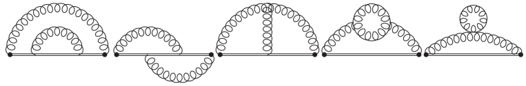
Figure 8: Diagrams contributing to $\delta\hat{q}_{\scriptscriptstyle L}\Big{|}_{\mathrm{loop}}$ at NLO.

$\delta\hat{q}_{\scriptscriptstyle L}\Big{|}_{\mathrm{subtr.}}^{\mathrm{diff}}$ arises from an $\mathcal{O}(g)$ error we have committed in the previous determination of $\hat{q}_{\scriptscriptstyle L}$ to LO. Namely, we have used and resummed HTL self-energies in the LO calculation, for instance, in Eq. (26), without worrying about the fact that the HTL loop integration extends down to zero momentum, where the hard approximations used to simplify the calculation of the HTL break down. In other words, the last two diagrams in Fig. 8 have already been included in our LO calculation, but using approximations which are invalid for small loop momentum. To fix this, we should subtract off the large-momentum limiting behavior of these diagrams when we evaluate them in the NLO computation.

We present the details of the calculation of both terms in App. F. Here we just mention that the general structure corresponds to what was found for the soft contribution to the photon rate Ghiglieri:2013gia . Schematically, the same sum-rule technology can be applied: the Wilson line propagators depend only on the minus components of the momenta, so that we can again deform the contour when integrating the plus component, which we call $q^{+}$. This corresponds to expanding those diagrams for large, complex $q^{+}$. The leading contribution should be of order $(q^{+})^{0}$ and the subleading one of order $(q^{+})^{-1}$. Higher-order terms are suppressed and can be neglected. The leading, $\mathcal{O}((q^{+})^{0})$ term, once integrated along the contour, will give rise to a linear divergence. An analogous linear divergence appears in $\delta\hat{q}_{\scriptscriptstyle L}\Big{|}^{\mathrm{coll}}_{\mathrm{subtr.}}$, as shown in Eq. (LABEL:collsoftct). As expected, these linear divergences cancel.

A term behaving as $\mathcal{O}(1/q^{+})$ at large $q^{+}$ has an interpretation of an asymptotic mass, which is why our LO result, Eq. (29), can be written in terms of the LO asymptotic mass. Therefore it is not surprising that the NLO correction is found by substituting the NLO form of the asymptotic mass $M_{\infty}^{2}\to M_{\infty}^{2}+\delta M_{\infty}^{2}$, as defined in Eq. (54), into Eq. (29), and then expanding to linear order in $\delta M_{\infty}^{2}$:

$$\frac{M_{\infty}^{2}}{q_{\perp}^{2}+M_{\infty}^{2}}\;\to\;\frac{M_{\infty}^{2}+\delta M_{\infty}^{2}}{q_{\perp}^{2}+M_{\infty}^{2}+\delta M_{\infty}^{2}}\simeq\frac{M_{\infty}^{2}}{q_{\perp}^{2}+M_{\infty}^{2}}+\delta M_{\infty}^{2}\frac{q_{\perp}^{2}}{(q_{\perp}^{2}+M_{\infty}^{2})^{2}}.$$ (79)

From Eq. (79) we thus obtain

$$\delta\hat{q}_{\scriptscriptstyle L}\Big{|}_{\mathrm{loop}}-\delta\hat{q}_{\scriptscriptstyle L}\Big{|}^{\mathrm{coll}}_{\mathrm{subtr.}}-\delta\hat{q}_{\scriptscriptstyle L}\Big{|}^{\mathrm{diff}}_{\mathrm{subtr.}}= g^{2}C_{R}T\int\frac{d^{2}q_{\perp}}{(2\pi)^{2}}\frac{q_{\perp}^{2}\delta M_{\infty}^{2}}{(q_{\perp}^{2}+M_{\infty}^{2})^{2}}$$

$$= \frac{g^{2}C_{R}T\delta M_{\infty}^{2}}{4\pi}\left[\ln\left(\frac{\left(\mu_{\perp}^{\mathrm{NLO}}\right)^{2}}{M_{\infty}^{2}}\right)-1\right].$$ (80)

This simpleminded argument indeed reproduces the detailed explicit calculation of Appendix F.

Eq. (80) depends on a regulator $\mu_{\perp}^{\mathrm{NLO}}$. As we will show, the dependence of this term on the regulator and the dependence of the semi-collinear region will cancel. This completes the evaluation of the diffusion sector to NLO.

7 Conversion processes at NLO

According to Eq. (43), the NLO corrections to the conversion sector take the following form:

$$\delta C_{a}^{\mathrm{conv}}[\delta\!f]=\sum_{b\neq a}\bigg{[}\delta\!f^{a}({\bm{p}})\delta\Gamma^{\mathrm{conv}}_{a\to b}(p)-\delta\!f^{b}({\bm{p}})\frac{d_{b}}{d_{a}}\delta\Gamma^{\mathrm{conv}}_{b\to a}(p)\bigg{]},$$ (81)

where the sum is understood to give rise to the structure of Eqs. (32)-(34). The NLO conversion rates are composed of three parts, namely

$$\delta\Gamma^{\mathrm{conv}}_{a\to b}(p)=\delta\Gamma^{\mathrm{conv}}_{a\to b}(p)\Big{|}_{\mathrm{loop}}-\delta\Gamma^{\mathrm{conv}}_{a\to b}(p)\Big{|}_{\mathrm{subtr.}}^{\mathrm{coll}}-\delta\Gamma^{\mathrm{conv}}_{a\to b}(p)\Big{|}_{\mathrm{subtr.}}^{\mathrm{conv}}.$$ (82)

The first term on the right-hand side comes from the soft-gluon loop correction to the rates, as defined by the Wilson-line operators (36)-(38). The second is the subtraction term from the collinear region, as obtained in Eq. (65), and the third subtracts the Hard Thermal Loop approximated leading-order calculation, result (3.3), in complete analogy to $\delta\hat{q}_{\scriptscriptstyle L}\big{|}_{\mathrm{subtr.}}^{\mathrm{diff}}$ encountered in the previous section.

The first and the third term can then be evaluated from Eqs. (36)-(38), by adding one extra soft gluon to the LO term in Eq. (3.3). A key observation is that the power-counting arguments that lead to the simplified form for $\hat{q}_{\scriptscriptstyle L}$ given by Eq. (78) apply here as well: all soft gluons must connect to the Wilson line as $r$ fields, so that their ordering is not relevant simonguy . This implies that the fundamental and adjoint Wilson lines appearing in Eqs. (36)-(38) can be simplified to NLO to a simpler antifundamental line connecting the soft fermionic fields, i.e.

$$\Gamma^{\mathrm{conv}}_{q\to g}(p) = -\frac{g^{2}C_{F}}{8d_{F}p}\int_{-\infty}^{+\infty}dx^{+}\left\langle\mathrm{Tr}\big{[}\bar{\psi}(x^{+},0,0_{\perp})\not{v}U_{F}(0,0,0;x^{+},0,0_{\perp})\psi(0)\big{]}\right\rangle,$$ (83)

$$\Gamma^{\mathrm{conv}}_{g\to q}(p) = \frac{d_{F}}{d_{A}}\Gamma^{\mathrm{conv}}_{q\to g}(p).$$ (84)

This corresponds to an effective abelianization of these operators, which, we note, are the same as those appearing in the fermionic sector of the Hard Thermal Loop action Braaten:1991gm . Indeed, an altogether similar abelianization happens for instance when obtaining the effective $qqg$ HTL vertex in QCD.

The diagrams necessary for the NLO evaluation of Eqs. (83) and (84) are shown in Fig. 9.

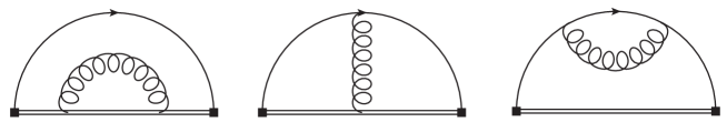
Figure 9: Diagrams obtained from Eq. (83) at NLO. The double line is the fundamental Wilson line and the black squares are the insertion of the soft fermion fields.

However, we note that, in their abelianized forms, Eqs. (83) and (84) correspond, up to the prefactors, to the soft-sector contribution to the NLO photon rate in Ghiglieri:2013gia . Therefore we can directly use that result, which was obtained using the same sum-rule techniques employed in the previous section. Indeed, as we observed there, the two results are remarkably similar, the only difference being given by the different asymptotic masses. Here the relevant one is the quark one and we then have

$$\delta\Gamma^{\mathrm{conv}}_{q\to g}(p)=\frac{g^{2}C_{F}}{4p}\int\frac{d^{2}q_{\perp}}{(2\pi)^{2}}\frac{q_{\perp}^{2}\,\delta m_{\infty}^{2}}{(q_{\perp}^{2}+m_{\infty}^{2})^{2}}=\frac{g^{2}C_{F}\delta m_{\infty}^{2}}{16\pi p}\left[\ln\left(\frac{\left(\mu_{\perp}^{\mathrm{NLO}}\right)^{2}}{m_{\infty}^{2}}\right)-1\right],$$ (85)

where $\delta m_{\infty}^{2}$ is given by Eq. (54) and the linear divergence in the collinear counterterm canceled an opposite one coming from the loop corrections. The logarithmic UV divergence has been treated with the same UV regulator $\mu_{\perp}^{\mathrm{NLO}}$ used in the previous section for $\delta\hat{q}_{\scriptscriptstyle L}$.

8 The semi-collinear region

As we anticipated in Sec. 4, semi-collinear processes can be seen as ${1\leftrightarrow 2}$ splitting processes where the virtuality and correspondingly the opening angle are larger. Two examples are drawn in Fig. 10.

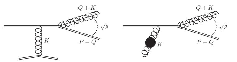
Figure 10: Diagrams for two typical semi-collinear processes. In the first case the soft gluon is in the space-like Landau cut, whereas in the second case it is on its time-like plasmon pole, represented by the black blob.

The scalings of this region are as follows: $K\sim gT$ is soft, whereas the two final-state particles are quasi-collinear, i.e. with an increased virtuality and opening angle with respect to the collinear sector. The leading contribution then comes from $q^{+}\sim T,\,q^{-}\sim gT,\,q_{\perp}^{2}\sim gT^{2}$, $Q^{2}\sim gT^{2}$ or, in the case of a democratic splitting, $q^{+}\sim E,\,q^{-}\sim gT,\,q_{\perp}^{2}\sim gTE$, $Q^{2}\sim gTE$. Naive power-counting arguments would suggest that the semi-collinear region should contribute to leading-order, as it is the largest slice of phase space where a soft gluon can attach to a ${1\leftrightarrow 2}$ process. However, once all diagrams are summed and squared, a cancellation, discussed in Arnold:2001ba in the context of photon radiation, introduces an extra $\mathcal{O}(g)$ suppression. Furthermore, as we shall show, the contribution from time-like soft gluons, e.g. plasmons, is now allowed.

The contribution $\delta C_{a}^{\mathrm{semi-coll}}$ to the collision operator can be written in the same way as the collinear one, as given by Eqs. (45)-(46), with the replacement of the collinear rates with semi-collinear ones. For instance, for quarks and antiquarks it reads

$$-\delta C_{q,\bar{q}}^{\mathrm{semi-coll}}[\delta\!f]({\bm{p}})= \int_{-\infty}^{+\infty}d\omega\delta\!f_{q,\bar{q}}((p+\omega)\hat{\bm{p}})\frac{d\Gamma^{q}_{qg}(p+\omega,\omega)}{d\omega}\Big{|}_{\mathrm{semi-coll}}$$

$$-\delta\!f_{q,\bar{q}}({\bm{p}})\frac{d\Gamma^{q}_{qg}(p,\omega)}{d\omega}\Big{|}_{\mathrm{semi-coll}}+\delta\!f_{g}((p+\omega)\hat{\bm{p}})\frac{d_{A}}{d_{F}}\frac{d\Gamma^{g}_{q\bar{q}}(p+\omega,\omega)}{d\omega}\Big{|}_{\mathrm{semi-coll}}.$$ (86)

The derivation of the semi-collinear rates then requires the evaluation of processes of the form of Fig. 10, with $p,q^{+}\gg q_{\perp}\gg k_{\perp},k^{+}$. Actually we have already evaluated these diagrams using the collinear expansion, since it is precisely these diagrams which give rise to the linear-in-collisions expressions we found in Subsec. 5.3.3. In particular, the subtraction term from the collinear region, Eq. (LABEL:colltosemi), was derived by making an expansion in $q^{+}\gg q_{\perp}$, and it still applies, under one condition. In evaluating the collision sector, we treated $q_{\perp}\sim k_{\perp}\sim gT$, leading to $\delta E\sim g^{2}T$. This let us neglect $\delta E$ when working out the kinematics of the soft gluons, so that ${\mathcal{C}}_{R}(k_{\perp})$ (see for instance Eq. (22)) is defined for $k^{-}=0$ and hence only space-like gluons contribute to it. But if $q_{\perp}^{2}\sim gT^{2},q^{+}\sim T$, or $q_{\perp}^{2}\sim gTE,q^{+}\sim E$, then $\delta E\sim gT$ and can no longer be neglected, opening up the time-like-gluon sector. In particular, when we put $(P-Q)$ and $(Q+K)$ on shell, we find, exactly as in the photon case Ghiglieri:2013gia , which we refer to for more details, that

$$\delta((Q+K)^{2})=\frac{\delta(k^{-}-\delta E)}{2|q^{+}|}+\mathcal{O}(\sqrt{g})\,,\qquad\delta E=\frac{p\,q_{\perp}^{2}}{2q^{+}(p-q^{+})}\approx\frac{p\,q_{\perp}^{2}}{2\omega(p-\omega)},$$ (87)

where the $\mathcal{O}(\sqrt{g})$ correction comes from $\mathbf{q}_{\perp}\cdot\mathbf{k}_{\perp}$ and always vanishes in the angular integrations. We see that $\delta E$ is exactly what we have used in Sec. 5.3.3. Therefore we must re-derive Eq. (LABEL:colltosemi) with these somewhat different kinematics. A straightforward computation shows that the findings in the case of photon radiation Ghiglieri:2013gia generalize to the present case. Namely, the quantity

$$\frac{\hat{q}}{g^{2}C_{R}}\equiv\frac{1}{g^{2}C_{R}}\int\frac{d^{2}k_{\perp}}{(2\pi)^{2}}\,k_{\perp}^{2}\,{\mathcal{C}}_{R}(k_{\perp})=\int\frac{d^{4}K}{(2\pi)^{3}}\delta(k^{-})k_{\perp}^{2}G_{rr}^{--}(K)\,,$$ (88)

physically interpreted as the transverse momentum diffusion coefficient and present in Eq. (LABEL:colltosemi), should be replaced with its finite $\delta E$ generalization,

$$\frac{\hat{q}(\delta E)}{g^{2}C_{R}}\equiv\int\frac{d^{4}K}{(2\pi)^{3}}\delta(k^{-}-\delta E)\left[k_{\perp}^{2}G^{--}_{rr}(K)+2G_{T}^{rr}(K)\left(\delta E^{2}-k^{+}\delta E\frac{k_{\perp}^{2}}{k^{2}}\right)\right],$$ (89)

which goes into Eq. (88) for $\delta E\to 0$ and corresponds to the leading-order soft term (in Coulomb gauge) in the evaluation of the operator

$$\hat{q}(\delta E)=\frac{g^{2}C_{R}}{d_{A}}\int_{-\infty}^{\infty}dx^{+}\,e^{ix^{+}\delta E}\,\langle v^{\mu}{F_{\mu}}^{\nu\,a}(x^{+},0,0_{\perp})U_{A}^{ab}(x^{+},0,0_{\perp};0,0,0_{\perp})v^{\rho}F^{b}_{\rho\nu}(0)\rangle,$$ (90)

which was first introduced in the photon case Ghiglieri:2013gia . In principle in the present case a more complicated “three-pole” operator should be needed CaronHuot:2008ni . However, at leading and next-to-leading order it would reduce to a set of three two-body exchanges of the form of (90), with the appropriate Casimir factors CaronHuot:2008ni .

Eq. (89) can be evaluated using Euclidean techniques, yielding Ghiglieri:2013gia

$$\frac{\hat{q}(\delta E)}{g^{2}C_{R}}=T\int\frac{d^{2}k_{\perp}}{(2\pi)^{2}}\bigg{[}\frac{m_{\scriptscriptstyle D}^{2}k_{\perp}^{2}}{(k_{\perp}^{2}+\delta E^{2})(k_{\perp}^{2}+\delta E^{2}+m_{\scriptscriptstyle D}^{2})}+\frac{2\delta E^{2}}{k_{\perp}^{2}+\delta E^{2}}\bigg{]}.$$ (91)

However, since this momentum region has overlap with both the collinear and the hard regions, there are two subtractions which must be conducted, corresponding to the treatments already included in those leading-order calculations. Therefore we must compute the behavior of this momentum region under each of those limiting kinematics and subtract them. The collinear case is treated by subtracting $\hat{q}$ from $\hat{q}(\delta E)$. For the hard region, we take the soft, bare limit ($n_{\scriptscriptstyle B}(k^{0})\to T/k^{0}$, $\rho(K)\to\rho^{(0)}(K)=2\pi\,\mathrm{sgn}(k^{0})\delta(K^{2})$) of Eq. (89), yielding

$$\frac{\hat{q}(\delta E)}{g^{2}C_{R}}\Big{|}_{\rm hard}\!=\int\frac{d^{4}K}{(2\pi)^{3}}\delta(k^{-}{-}\delta E)2G_{T}^{(0)rr}(K)\delta E^{2}=T\int\frac{d^{2}k_{\perp}}{(2\pi)^{2}}\frac{2\delta E^{2}}{k_{\perp}^{2}+\delta E^{2}},$$

The full semi-collinear rate is then obtained by replacing

$$\frac{\hat{q}}{g^{2}C_{R}}\to\frac{\hat{q}(\delta E)}{g^{2}C_{R}}-\frac{\hat{q}}{g^{2}C_{R}}-\frac{\hat{q}(\delta E)}{g^{2}C_{R}}\Big{|}_{\rm hard},$$ (92)

in Eq. (LABEL:colltosemi), which yields

$$\frac{d\Gamma(p,\omega)}{d\omega}\Big{|}_{\mathrm{semi-coll}}= \frac{g^{4}C_{R}T}{2\pi p}(1\pm n(\omega))(1\pm n(p-\omega))\int\frac{d^{2}q_{\perp}}{(2\pi)^{2}}\int\frac{d^{2}k_{\perp}}{(2\pi)^{2}}\frac{1}{q_{\perp}^{4}}$$

$$\times\left\{\begin{array}[]{cc}\frac{1+(1-x)^{2}}{x}\big{[}C_{F}x^{2}+C_{A}(1-x)\big{]}&q\to qg\\ \frac{d_{F}}{d_{A}}(x^{2}+(1-x)^{2})\big{[}C_{F}+C_{A}x(1-x)\big{]}&g\to q\bar{q}\\ \frac{1+x^{4}+(1-x)^{4}}{x(1-x)}C_{A}\big{[}1-x+x^{2}\big{]}&g\to gg\end{array}\right\}$$ (96)

$$\times\bigg{[}\frac{m_{\scriptscriptstyle D}^{2}k_{\perp}^{2}}{(k_{\perp}^{2}+\delta E^{2})(k_{\perp}^{2}+\delta E^{2}+m_{\scriptscriptstyle D}^{2})}-\frac{m_{\scriptscriptstyle D}^{2}}{k_{\perp}^{2}+m_{\scriptscriptstyle D}^{2}}\bigg{]}.$$ (97)

We stress that the collision operator has the same form as Eqs. (45)-(46).

The $q_{\perp}$ integration in Eq. (97) is to be understood as IR-regulated by $\mu_{\perp}^{\mathrm{NLO}}$. In App. G we show how the small-$\omega$-and-$q_{\perp}$ region gives rise to IR logarithms that cancel the $\mu_{\perp}^{\mathrm{NLO}}$ dependence of the diffusion and conversion sectors. We also give some details of how the transverse integrations can be carried out analytically. The $\omega$ integration remains to be performed numerically.

9 Summary and conclusions

The main aim of this paper has been to show how the propagation of highly energetic quarks and gluons through the QGP can be described at leading- and next-to-leading order by a Boltzmann equation encoding the interaction between these hard particles and the thermal and soft constituents of the plasma. Sec. 2 has been devoted to a brief review of the LO kinetic approach introduced in Arnold:2002zm and implemented in MARTINI. As Eq. (1) summarizes, the two processes it incorporates are ${2\leftrightarrow 2}$ scatterings with the thermal medium constituents and ${1\leftrightarrow 2}$ collinear splittings induced by the soft background.

In Sec. 3 we have shown how this approach is not optimal beyond leading order, where the distinction between the two classes would blur and the resummed matrix-element approach to ${2\leftrightarrow 2}$ scattering would become cumbersome. With these motivations, we have reorganized the LO collision operator into four separate processes which provide a sufficient description at NLO. They are large-angle scatterings, i.e. ${2\leftrightarrow 2}$ scatterings with $\mathcal{O}(1)$ angles or equivalently $\mathcal{O}(T)$ or larger transferred momentum, diffusion processes, caused by soft gluon exchanges, which preserve the identity of the hard particles while slightly affecting their momentum, conversion processes which instead turn quarks into gluons and vice versa through soft quark exchange and finally collinear processes, corresponding at LO to ${1\leftrightarrow 2}$ processes. In Sec. 3.1 we described in detail our description of large-angle processes, which require regularization to be kept separate from diffusion and conversion ones, as shown in Eqs. (13) and (15). Sec. 3.2 has been dedicated to diffusion processes, which are described by an effective Fokker-Planck equation, Eq. (16). The three physical effects of drag (energy loss), longitudinal and transverse momentum broadening are encoded in three corresponding coefficients. The requirements that the Fokker-Planck picture be equivalent to the Boltzmann one and that it approach equilibrium can be used to write the drag coefficient in terms of the other two, as per Eq. (30). The two momentum diffusion coefficients can then effectively be described by field strength correlators along Wilson lines on the light-cone direction of propagation of the hard particle, as in Eq. (24). The calculation of the transverse momentum diffusion coefficient $\hat{q}$ is mapped to a Euclidean one CaronHuot:2008ni , whereas for the longitudinal momentum diffusion coefficient $\hat{q}_{\scriptscriptstyle L}$ we introduce a sum rule which, through the analytical properties of amplitudes at light-like separations, makes it sensitive only to the gluon dispersion relation close to the light cone (see Eq. (29)). Similarly, conversion processes are shown in Sec. 3.3 to be described by effective Wilson line operators (Eqs. (36) and (37)), which are also computed through an equivalent light-cone sum rule mapping them to the quark dispersion relation. The UV log-divergence of the diffusion and conversion processes cancels with the opposite IR one in large-angle scatterings.

In Sec. 4 we introduced the NLO extension of this reorganized approach. All processes, with the exception of large-angle scatterings, are sensitive to $\mathcal{O}(g)$ corrections arising from the interactions with the soft background. Furthermore, some care is necessary in avoiding double countings in slices of the phase space, which were included at LO, where some particles become soft, introducing the need for a set of subtractions. The remaining sections are then devoted to the details of each process at NLO. In Sec. 5 we discuss the collinear region, which is sensitive to $\mathcal{O}(g)$ corrections in the interactions with the soft background that induce the splitting, as well as in the dispersion relation of the hard and thermal particles. We further identify all necessary subtractions.

Sec. 6 is dedicated to $\mathcal{O}(g)$ corrections to diffusion. In treating $\hat{q}$, we employ the NLO determination of CaronHuot:2008ni , whereas for $\hat{q}_{\scriptscriptstyle L}$ we perform the calculation using the light-cone sum rules introduced before. The details are to be found in App. F. The result is surprisingly simple: it just amounts to considering the soft correction to the gluon dispersion relation close to the light-cone (see Eq. (79)). Similarly, conversion processes are dealt with using the fermionic analogue of the same sum rule and require the inclusion of the soft correction to the quark asymptotic mass, as in Eq. (85). Both $\hat{q}_{\scriptscriptstyle L}$ and the conversion rate at NLO show an UV logarithmic divergence, which is removed once a new process, which only starts to contribute at NLO, is considered, the semi-collinear process. As illustrated in Sec. 8, this process appears as a bridge between the diffusion/conversion sector on one side and the collinear on the other. Indeed, while retaining a collinear kinematics, it shows relaxed constraints, going beyond strict collinearity and allowing the interactions with the soft background to be not just space-like (soft scatterings) but also time-like (plasmon absorption/emission). For its evaluation a modified form of $\hat{q}$, $\hat{q}(\delta E)$, is introduced in Eq. (90). It accounts for the changes in the small light-cone component $p^{-}$, which are no longer negligible. Euclidean techniques are used for its computation, as per Eq. (91).

We would like to emphasize the importance of Euclidean techniques, which map the calculation of ${\mathcal{C}}(k_{\perp})$, $\hat{q}$, $\hat{q}(\delta E)$, $\delta M_{\infty}^{2}$ and $\delta m_{\infty}^{2}$ into simpler calculations in dimensionally-reduced EQCD. Similarly, light-cone sum rules reduce the computation of $\hat{q}_{\scriptscriptstyle L}$ and of the conversion rates to the determination of the gluon and quark asymptotic masses at leading- and next-to-leading order. Without these recent theoretical developments, rooted in the causal properties of amplitudes at light-like separations, the calculations presented here would have required extensive, cumbersome numerical integrations over the intricate structures of loops composed of HTL propagators and vertices. Furthermore, as we have mentioned, Euclidean techniques also allow lattice determinations. The first measurements of $\hat{q}$ and ${\mathcal{C}}(x_{\perp})$ have recently been reported Laine:2013lia ; Panero:2013pla , opening up a new avenue of research. All other Euclidean operators can be computed on the lattice in the same way, creating the tantalizing possibility of a factorized approach to kinetics, where perturbation theory is used at the thermal and hard scales to compute the large-angle scatterings and the splittings, whereas the 3D lattice is employed at the soft (and ultrasoft) scale to determine non-perturbatively the transverse diffusion processes and the scatterings leading to collinear radiation.

A very important point we have not addressed in this paper, leaving it to future work, is the impact of the NLO corrections we have introduced on calculations of jet modification and their comparison to experimental data. As we mentioned, the Monte Carlo event generator MARTINI implements a kinetic approach corresponding to the one described in Sec. 2. This makes it an ideal candidate for the inclusion of the NLO corrections. Indeed, the reorganization of the LO collision operator in terms of large-angle, diffusion, conversion and collinear processes is underway, as well as the implementation of the NLO corrections. This could also be easily complemented by the inclusion of non-perturbative input, such as the existing determination of $\hat{q}$ and, should they become available, future determinations of $\hat{q}(\delta E)$ and of the asymptotic masses. It would also be interesting to study the angular structures of jets with this numerical implementation and compare it with the recent order-of-magnitude perturbative estimates from Kurkela:2014tla .

We remark that it is difficult for us to gauge a priori the impact of NLO corrections relative to LO. The recent NLO calculations of the thermal photon Ghiglieri:2013gia and low-mass dilepton Ghiglieri:2014kma rates, which include many of the features presented here, such as Euclidean techniques, light-cone sum rules, semi-collinear and collinear processes, showed how the NLO corrections naturally grouped into two classes of large, and largely canceling, contributions. The positive corrections were due to NLO modifications to the collinear processes, caused by the increased soft scattering rate and the reduced asymptotic masses, while semi-collinear and conversion processes decreased the rate by a similar magnitude. The large cancellation between these contribution is mostly accidental and furthermore depends significantly on the details of the medium, such as the numbers of colors and flavors. So, while we anticipate similar cancellations for the present energy loss case, we are at present unable to quantify their impact in more detail.

Finally, we believe that the approach presented here should go much of the way towards making possible NLO kinetic theory calculations of the shear viscosity and other transport coefficients of QCD. However, we have not resolved the issue of keeping track of where the energy from a soft scattering shows up amongst the other (thermal) particles, which so far prevents us from a true NLO calculation of QCD transport coefficients. We hope to return to this issue in the future. We do note, however, that for cases where the momentum dependence of the off-equilibrium distributions is isotropic, such as studies of isotropic thermalization York:2014wja ; Kurkela:2014tea , an extension to NLO appears within reach.

Appendix A Notation

We now summarize our notation. We will use capital letters for four-vectors, lowercase italic letters for the modulus of the spatial three-vectors, and the mostly-plus metric $\eta_{\mu\nu}=\mathrm{Diag}\>[{-}{+}{+}{+}]$, so that $P^{2}=p^{2}-p^{2}_{0}$.

For convenience we will mostly work in the Keldysh, or $r,a$ , basis of the real-time formalism for the computation of thermal expectation values. The two elements of this basis are defined as $\phi_{r}\equiv(\phi_{1}+\phi_{2})/2$, $\phi_{a}\equiv\phi_{1}-\phi_{2}$, $\phi$ being a generic field and the subscripts 1 and 2 labeling the time-ordered and anti-time-ordered branches of the Schwinger-Keldysh contour respectively. The propagator is a $2\times 2$ matrix, where one entry is always zero and only one entry depends on the thermal distribution, i.e.,

$$D=\left(\begin{array}[]{cc}D_{rr}&D_{ra}\\ D_{ar}&D_{aa}\end{array}\right)=\left(\begin{array}[]{ccc}\left(\frac{1}{2}\pm n(p^{0})\right)(D_{R}-D_{A})&&D_{R}\\ D_{A}&&0\end{array}\right),$$ (98)

where $D_{R}$ and $D_{A}$ are the retarded and advanced propagators, the plus (minus) sign refers to bosons (fermions). $n(p^{0})$ is the corresponding thermal distribution, either $n_{\scriptscriptstyle B}(p^{0})=(\exp(p^{0}/T)-1)^{-1}$ for bosons or $n_{\scriptscriptstyle F}(p^{0})=(\exp(p^{0}/T)+1)^{-1}$ for fermions. We also define the spectral function as the difference of the retarded and advanced propagators, $\rho\equiv D_{R}-D_{A}$. We will denote the gluon propagator by $G$ and the quark one $S$.

We will adopt strict Coulomb gauge throughout. The treatment of soft momenta in propagators and vertices requires the use of Hard Thermal Loop (HTL) resummation Braaten:1989mz . For convenience we list the Coulomb gauge retarded HTL resummed propagators for fermions and gluons in the next section.

Appendix B Hard Thermal Loop propagators

In this section we detail our conventions for the HTL propagators. Fermion propagators are most easily written in terms of components with positive and negative chirality-to-helicity ratio. The retarded fermion propagator reads

$$S_{R}(P)=h^{+}_{\bm{p}}S^{+}_{R}(P)+h^{-}_{\bm{p}}S^{-}_{R}(P)\,,$$ (99)

where

$$S^{\pm}_{R}(P)=\frac{i}{p^{0}\mp(p+\Sigma^{\pm}(p^{0}/p))}=\left.\frac{i}{\displaystyle p^{0}\mp\left[p+\frac{m_{\infty}^{2}}{2p}\left(1-\frac{p^{0}\mp p}{2p}\ln\left(\frac{p^{0}+p}{p^{0}-p}\right)\right)\right]}\right|_{p^{0}=p^{0}+i\epsilon},$$ (100)

where the upper (lower) sign refers to the positive (negative) chirality-to-helicity component. The projectors are $h^{\pm}_{\bm{p}}\equiv(\gamma^{0}\mp\vec{\gamma}\cdot\hat{p})/2$. Here $m_{\infty}^{2}$ is the fermionic asymptotic mass squared, defined such that the large-momentum dispersion relation for helicity=chirality fermions is $p_{0}^{2}=p^{2}+m_{\infty}^{2}$. We similarly define the asymptotic gluonic mass $M_{\infty}^{2}$. At leading order, their values are

$$M_{\infty}^{2}=\frac{m_{\scriptscriptstyle D}^{2}}{2}=\frac{g^{2}T^{2}}{6}\left(N_{c}+\frac{N_{f}}{2}\right),\qquad m_{\infty}^{2}=2m_{q}^{2}=C_{F}\frac{g^{2}T^{2}}{4},$$ (101)

where we have also shown the relations to the more commonly used Debye mass $m_{\scriptscriptstyle D}$ and quark “mass” $m_{q}$.

Gluons are described in the strict Coulomb gauge by

$$G^{00}_{R}(Q) = \frac{i}{\displaystyle q^{2}+m_{\scriptscriptstyle D}^{2}\left(1-\frac{q^{0}}{2q}\ln\frac{q^{0}+q+i\epsilon}{q^{0}-q+i\epsilon}\right)},$$ (102)

$$G^{ij}_{R}(Q) = (\delta^{ij}-\hat{q}^{i}\hat{q}^{j})G^{T}_{R}(Q)=\left.\frac{i(\delta^{ij}-\hat{q}^{i}\hat{q}^{j})}{\displaystyle q_{0}^{2}-q^{2}-M_{\infty}^{2}\left(\frac{q_{0}^{2}}{q^{2}}-\left(\frac{q_{0}^{2}}{q^{2}}-1\right)\frac{q^{0}}{2q}\ln\frac{q^{0}{+}q}{q^{0}{-}q}\right)}\right|_{q^{0}=q^{0}+i\epsilon}.$$

The other components of the propagators in the $r,a$ basis can be obtained through Eq. (98).

Appendix C Longitudinal momentum diffusion from Wilson lines

Eq. (24) is based on eikonalization, which naturally happens since $p$ is considered infinitely larger than all other scales at leading order. As such, it can be easily verified that the perturbative expansion of Eq. (24) agrees with the rate-based definition (19) at leading and next-to-leading order. We believe that, in the presence of a consistent UV regulator Eq. (24) is correct to all orders in $g$ at the leading order in $1/p$, up to possible Wilson lines along the $x^{-}$ direction at $x^{+}=-\infty$. Indeed, we believe that Eq. (24) can be rigorously obtained in dimensional regularization using SCET, analogously to what has been done in D'Eramo:2010ak ; Benzke:2012sz for $\hat{q}$. We sketch here a simplistic derivation. Since we are interested in the differential-in-$q^{z}$ rate for a fast particle propagating with $p^{0}=p^{z}$, it is natural to expect from the eikonal approximation a correlator of the form

$$(2\pi)\frac{d\Gamma}{dq^{z}}=(2\pi)\frac{d\Gamma}{dq^{+}}=\lim_{L\to\infty}\frac{1}{L}\int dx^{-}e^{iq^{+}x^{-}}\frac{1}{d_{R}}\big{\langle}\mathrm{Tr}U(-L/2,L/2;x^{-})U(L/2,-L/2;0)\big{\rangle},$$ (104)

where we have used the fact that in the infinite-$p$ limit $q^{z}=q^{+}$ and for simplicity we have introduced

$$U(a^{+},b^{+};c^{-})=P\exp\left(ig\int_{b^{+}}^{a^{+}}dl^{+}A^{-}(l^{+},c^{-})\right),$$ (105)

and for further convenience

$$\tilde{U}(a^{-},b^{-};c^{+})=P\exp\left(ig\int_{b^{-}}^{a^{-}}dl^{-}A^{+}(l^{-},c^{+})\right).$$ (106)

The Wilson line at $x^{-}=0$ is supported on the time-ordered branch of the Schwinger-Keldysh contour and conversely the other one is supported on the anti-time ordered branch, corresponding to the amplitude and conjugate amplitude entering the definition of the rate. Indeed, so far the techniques used in D'Eramo:2010ak ; Benzke:2012sz are exactly applicable here as well, so that Eq. (104) is also formally justified within SCET. It is however not gauge-invariant. Following the steps of Benzke:2012sz , we conjecture this form for its gauge-invariant dressing:

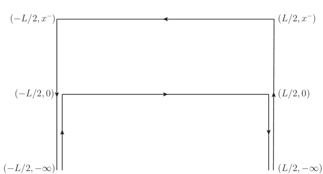
Figure 11: The Wilson loop giving rise to $\hat{q}_{\scriptscriptstyle L}$. The horizontal axis is the $+$ axis and the vertical one is the $-$ one. The points are given in $(x^{+},x^{-})$ coordinates, the constant transverse one is not shown.

$$(2\pi)\frac{d\Gamma}{dq^{+}} = \lim_{L\to\infty}\frac{1}{L}\int dx^{-}e^{iq^{+}x^{-}}\frac{1}{d_{R}}\big{\langle}\mathrm{Tr}\tilde{U}(-\infty,x^{-};-L/2)U(-L/2,L/2;x^{-})$$ (107)

$$\times\tilde{U}(x^{-},-\infty;L/2)\tilde{U}(-\infty,0;L/2)U(L/2,-L/2;0)\tilde{U}(0,-\infty;-L/2)\big{\rangle}.$$

The operator defined by Eq. (107) is sketched in Fig. 11. This particular ordering corresponds to having the upper three connected Wilson lines on the anti-time ordered branch of the Schwinger-Keldysh contour and the lower three on the time-ordered one. The “handle” on the bottom right corner can be trivially annihilated, but the same is not true for the one at the bottom left, since time-like separated fields appear between the two vertical Wilson lines there.

Finally, by using the definition of $\hat{q}_{\scriptscriptstyle L}$ and convoluting Eq. (107) with $(q^{+})^{2}$, the latter can be replaced by derivatives which, when acting on the Wilson loop, introduce the $F^{+-}$ electric fields. Once the $q^{+}$ integration is taken (with infinite cutoff, hence the strict validity in dimensional regularization only), the Wilson line operator (107) is squeezed to the form of Eq. (24) plus a surviving “handle” along $x^{-}$ at $x^{+}=-\infty$. This handle is irrelevant in non-singular gauges and even in the light-cone gauge $A^{-}=0$ it can be neglected at LO and NLO. The same would not be true for $dp_{\scriptscriptstyle L}/dt$ (in the $p\to\infty$ limit), where we would encounter a single $F^{+-}$ insertion (at $x^{+}$) and the handle would be critical in obtaining a gauge-invariant leading-order result.

Appendix D Leading-order matching

In this section we shall prove how the diffusion+conversion+large-angle scattering is equivalent to the dressed ${2\leftrightarrow 2}$ processes of Arnold:2002zm .

D.1 Diffusion matching

For simplicity, we only consider diffusion matching for the $q_{1}q_{2}\leftrightarrow q_{1}q_{2}$ contribution previously illustrated in Eq. (10). In the prescription of Arnold:2002zm , that process is treated by using the identity

$$\frac{s^{2}{+}u^{2}}{t^{2}}=\frac{1}{2}+\frac{1}{2}\,\frac{(s{-}u)^{2}}{t^{2}}\,,$$ (108)

and the replacement

$$\frac{(s{-}u)^{2}}{t^{2}}\longrightarrow\left|G^{R}_{\mu\nu}(P{-}P^{\prime})(P{+}P^{\prime})^{\mu}(K{+}K^{\prime})^{\nu}\right|^{2},$$ (109)

where $G^{R}(Q)$ is the retarded HTL propagator, as given by Eqs. (102) and (LABEL:htltrans). Upon plugging this into Eq. (13), putting the IR regulator to zero, introducing instead an UV regulator $T\gg\mu_{\tilde{q}_{\perp}}\gg gT$ and consistently expanding for $\omega,\tilde{q}_{\perp}\sim gT$, we get

$$C_{q_{1}}^{\mathrm{large}}[\delta\!f] \supset \frac{C_{F}g^{4}}{32\pi^{3}}\int_{-\infty}^{+\infty}d\omega\int_{0}^{\mu_{\tilde{q}_{\perp}}}d\tilde{q}_{\perp}\frac{\tilde{q}_{\perp}}{q}\int_{0}^{\infty}dkn_{\scriptscriptstyle F}(k)\,[1-n_{\scriptscriptstyle F}(k)]\times$$

$$\left\{\left(2\left|G^{L}_{R}(Q)\right|^{2}+\frac{\tilde{q}_{\perp}^{4}}{q^{4}}\left|G^{T}_{R}(Q)\right|^{2}\right)k\left[k+\omega\left(1-\frac{k}{p}\right)\right]+\mathcal{O}\left(\omega^{2},\tilde{q}_{\perp}^{2}\right)\right\}\times$$

$$\left[\frac{\omega T-\omega^{2}(1{-}2n_{\scriptscriptstyle F}(k))}{2T^{2}}\delta\!f^{q_{1}}(p)+\frac{\omega T-\omega^{2}(1{-}n_{\scriptscriptstyle F}(k))}{T}\frac{d\delta\!f^{q_{1}}(p)}{dp}-\frac{\omega^{2}}{2}\frac{d\delta\!f^{q_{1}}(p)}{dp^{2}}\right],$$

where $G(Q)$ is understood to be $G(\omega,q=\sqrt{\omega^{2}+\tilde{q}_{\perp}^{2}})$ and we have omitted the stimulation factor and its derivatives on the outgoing hard leg, as they are all exponentially suppressed. Up to higher-order corrections we can put the lower integration limit for the $k$ integration to zero. The terms within the first set of curly brackets come from the expansion of the $\phi$-averaged matrix element, whereas those in the second set come from the expansion of the distribution functions. We remark that the square moduli of the propagators on the first line are even functions of $\omega$. Hence, the terms that would naively be of leading order in this expansion in $g$, i.e. those multiplying $\delta\!f$ and its first derivative on the third line, vanish in the integration. Keeping only the surviving, even-in-$\omega$ pieces and performing the $k$ integration we have

$$C_{q_{1}}^{\mathrm{large}}[\delta\!f] \supset -\frac{g^{2}T^{2}}{6}\frac{C_{F}g^{2}}{32\pi^{2}}\int_{-\infty}^{+\infty}d\omega\int_{0}^{\mu_{\tilde{q}_{\perp}}}d\tilde{q}_{\perp}\,\tilde{q}_{\perp}\frac{\rho^{--}(Q)}{m_{\scriptscriptstyle D}^{2}\omega}$$ (111)

$$\times\omega^{2}\Bigg{\{}\delta\!f^{q_{1}}(p)\,\frac{2}{p}+\frac{d\delta\!f^{q_{1}}(p)}{dp}\left[\left(1+\frac{2T}{p}\right)\right]+T\frac{d\delta\!f^{q_{1}}(p)}{dp^{2}}\Bigg{\}}.$$

where we have also used the following relations, based on the explicit form of the propagator in Eqs. (102) and (LABEL:htltrans):

$$\rho^{L}(Q) = G^{L}_{R}(Q)-G^{L}_{A}(Q)=\pi m_{\scriptscriptstyle D}^{2}\frac{\omega}{q}\left|G^{L}_{R}\right|^{2},$$

$$\rho^{T}(Q) = G^{T}_{R}(Q)-G^{T}_{A}(Q)=\pi m_{\scriptscriptstyle D}^{2}\frac{\omega}{2q}\left(1-\frac{\omega^{2}}{q^{2}}\right)\left|G^{T}_{R}\right|^{2}.$$ (112)

We also remark that the next terms in the soft expansion, i.e. those $\mathcal{O}(\omega^{2},\tilde{q}_{\perp}^{2})$, which naively would contribute to relative $\mathcal{O}(g)$, give rise again to a vanishing odd integration and thus contribute only to $\mathcal{O}(g^{2})$. For this reason they can be neglected. Similarly, the next order in the expansion of the distribution function is also odd and vanishes. Hence, a genuine $\mathcal{O}(g)$ correction can only arise from adding soft gluons to these diagrams.

An analogous expression can be obtained in the case of a ${\bm{p}}$-dependent $\delta\!f$. It reads

$$C_{q_{1}}^{\mathrm{large}}[\delta\!f] \supset -\frac{g^{2}T^{2}}{6}\frac{C_{F}g^{2}}{32\pi^{2}}\int_{-\infty}^{+\infty}d\omega\int_{0}^{\mu_{\tilde{q}_{\perp}}}d\tilde{q}_{\perp}\,\tilde{q}_{\perp}\frac{\rho^{--}(Q)}{m_{\scriptscriptstyle D}^{2}\omega}$$ (113)

$$\times\Bigg{\{}\delta\!f^{q_{1}}({\bm{p}})\,\omega^{2}\frac{2}{p}+\frac{d\delta\!f^{q_{1}}({\bm{p}})}{dp^{z}}\left[\omega^{2}\left(1+\frac{2T}{p}\right)-\frac{T}{p}\tilde{q}_{\perp}^{2}\right]$$

$$+T\left(\omega^{2}\frac{d\delta\!f^{q_{1}}({\bm{p}})}{d(p^{z})^{2}}+\frac{\tilde{q}_{\perp}^{2}}{2}\nabla^{2}_{p_{\perp}}\delta\!f^{q_{1}}({\bm{p}})\right)\Bigg{\}}.$$

Now let us look at the coefficients entering Eq. (16), as defined in Eqs.(18), (19) and (20). The differential rates appearing there can be easily inferred from the loss term of the collision operator (10). Applying the same steps that led to Eq. (D.1) we have that the contribution from scattering with a quark $q_{2}$ to $dp_{\scriptscriptstyle L}/dt$ for a quark reads

$$\frac{dp_{\scriptscriptstyle L}}{dt}\Big{|}_{q_{1}} \supset -\frac{g^{4}}{(2\pi)^{3}}\frac{C_{F}}{4}\int_{-\infty}^{+\infty}d\omega\int_{0}^{\mu_{\tilde{q}_{\perp}}}d\tilde{q}_{\perp}\frac{\tilde{q}_{\perp}}{q}\int_{0}^{\infty}dk\,q^{z}\Bigg{\{}\left(2\left|G^{L}_{R}(Q)\right|^{2}+\frac{\tilde{q}_{\perp}^{4}}{q^{4}}\left|G^{T}_{R}(Q)\right|^{2}\right)$$ (114)

$$\times k\left[k+\omega\left(1-\frac{k}{p}\right)\right]+\mathcal{O}\left(\omega^{2},\tilde{q}_{\perp}^{2}\right)\Bigg{\}}n_{\scriptscriptstyle F}(k)\,[1-n_{\scriptscriptstyle F}(k+\omega)],$$

where we have for clarity left the stimulation factor $[1-n_{\scriptscriptstyle F}(k+\omega)]$ unexpanded in $\omega\sim g$. Using Eq. (14), i.e. $q^{z}=\omega+\tilde{q}_{\perp}^{2}/(2p)$, one sees again that the naive leading order in $g$ leads to a vanishing $\omega$ integration, which is at the base of the Einstein relation relating $dp_{\scriptscriptstyle L}/dt$ and $\hat{q}_{\scriptscriptstyle L}$ in the $p\to\infty$ limit. The leading, even-in-$\omega$ terms then yield, upon performing the $k$ integration and using again Eq. (112)

$$\frac{dp_{\scriptscriptstyle L}}{dt}\Big{|}_{q_{1}}\supset-\frac{g^{2}T^{2}}{6}\frac{C_{F}g^{2}}{32\pi^{2}}\int_{-\infty}^{+\infty}d\omega\int_{0}^{\mu_{\tilde{q}_{\perp}}}d\tilde{q}_{\perp}\,\tilde{q}_{\perp}\frac{\rho^{--}(Q)}{m_{\scriptscriptstyle D}^{2}\omega}\left[\omega^{2}\left(1-\frac{2T}{p}\right)+\tilde{q}_{\perp}^{2}\frac{T}{p}\right],$$ (115)

where we have again not considered the $\mathcal{O}(g^{2})$ correction from the $\mathcal{O}(\omega^{2},\tilde{q}_{\perp}^{2})$ terms in the expansion of the matrix elements and from the expansion of the distribution functions.

Returning to $\hat{q}_{\scriptscriptstyle L}$, it is immediate to see that, at leading order, only the $\omega^{2}$ term in $(q^{z})^{2}$ contributes and other terms are actually suppressed by a factor of $g^{2}$. Hence $\hat{q}_{\scriptscriptstyle L}$ reads at LO

$$\hat{q}_{\scriptscriptstyle L}\Big{|}_{q_{1}}\supset\frac{g^{2}T^{3}}{6}\frac{C_{F}g^{2}}{16\pi^{2}}\int_{-\infty}^{+\infty}d\omega\int_{0}^{\mu_{\tilde{q}_{\perp}}}d\tilde{q}_{\perp}\,\tilde{q}_{\perp}\,\omega^{2}\frac{\rho^{--}(Q)}{m_{\scriptscriptstyle D}^{2}\omega}.$$ (116)

Similarly, for $\hat{q}$ one has $q_{\perp}^{2}=\tilde{q}_{\perp}^{2}$, up to odd corrections or $\mathcal{O}(g^{2})$ terms, so that one obtains the well known result (see Eq. (23))

$$\hat{q}\Big{|}_{q_{1}}\supset\frac{g^{2}T^{3}}{6}\frac{C_{F}g^{2}}{16\pi^{2}}\int_{-\infty}^{+\infty}d\omega\int_{0}^{\mu_{\tilde{q}_{\perp}}}d\tilde{q}_{\perp}\,\tilde{q}_{\perp}\,\tilde{q}_{\perp}^{2}\frac{\rho^{--}(Q)}{m_{\scriptscriptstyle D}^{2}\omega}.$$ (117)

We furthermore remark that in $\hat{q}_{\scriptscriptstyle L}$ and $\hat{q}$ corrections in $1/p$ enter only at $\mathcal{O}(g^{2})$, due again to the $\mathcal{O}(g)$ term being odd in $\omega$. For this same reason the evaluation in $(\omega,\tilde{q}_{\perp})$ and $(q^{+},q_{\perp})$ coordinates is equivalent. This justifies our evaluation of the ($p$-independent) NLO corrections to $\hat{q}_{\scriptscriptstyle L}$ and $\hat{q}$ in the latter coordinate set.

Let us obtain the complete leading-order $dp_{\scriptscriptstyle L}/dt$, $\hat{q}_{\scriptscriptstyle L}$ and $\hat{q}$. To this end, one has $2(N_{f}-1)$ quarks and antiquarks that are distinguishable from $q_{1}$, and hence $4(N_{f}-1)$ contributions in the form of Eqs. (115), (116) and (117), the extra factor of $2$ coming from the sum over final states (see footnote 5). The contribution from $q_{1}q_{1}$ scattering accounts for two times those equations, as the $u$-channel contribution is identical, and the $q_{1}\bar{q}_{1}$ accounts for another two due again to final state symmetries. Hence the contribution from all quark scatterings account for a factor of $4N_{f}$. Using altogether similar steps one can show that the contribution from $q_{1}g$ scatterings amounts to a factor of $8N_{c}$, so that the complete leading-order expressions are

$$\frac{dp_{\scriptscriptstyle L}}{dt}\Big{|}_{q} = -\frac{C_{F}g^{2}}{8\pi^{2}}\int_{-\infty}^{+\infty}d\omega\int_{0}^{\mu_{\tilde{q}_{\perp}}}d\tilde{q}_{\perp}\,\tilde{q}_{\perp}\frac{\rho^{--}(Q)}{\omega}\left[\omega^{2}\left(1-\frac{2T}{p}\right)+\tilde{q}_{\perp}^{2}\frac{T}{p}\right],$$ (118)

$$\hat{q}_{\scriptscriptstyle L}\Big{|}_{q} = \frac{C_{F}g^{2}}{4\pi^{2}}\int_{-\infty}^{+\infty}d\omega\int_{0}^{\mu_{\tilde{q}_{\perp}}}d\tilde{q}_{\perp}\,\tilde{q}_{\perp}\,\omega^{2}\frac{T}{\omega}\rho^{--}(Q),$$ (119)

$$\hat{q}\Big{|}_{q} = \frac{C_{F}g^{2}}{4\pi^{2}}\int_{-\infty}^{+\infty}d\omega\int_{0}^{\mu_{\tilde{q}_{\perp}}}d\tilde{q}_{\perp}\,\tilde{q}_{\perp}\,\tilde{q}_{\perp}^{2}\frac{T}{\omega}\rho^{--}(Q),$$ (120)

which agree with Eqs. (29) and (23). In the case where the hard particle is a gluon, one obtains the same expressions with $C_{F}$ replaced by $C_{A}$.

We can now see explicitly, by comparing Eqs. (118), (119) and (120), that the equilibration condition Eq. (30) is obeyed at leading order. Finally, let us take Eq. (16), and substitute the equilibration condition. This yields, for a $p$-dependent $\delta\!f$,

$$C_{a}^{\mathrm{diff}}[\delta\!f]=-\frac{\hat{q}_{\scriptscriptstyle L}}{Tp}\delta\!f(p)-\frac{d\delta\!f(p)}{dp}\hat{q}_{\scriptscriptstyle L}\left(\frac{1}{p}+\frac{1}{2T}\right)-\frac{1}{2}\hat{q}_{\scriptscriptstyle L}\frac{d^{2}\delta\!f(p)}{dp^{2}},$$ (121)

which matches with the structure of Eq. (111). In the ${\bm{p}}$-dependent case we recover instead Eq. (31), which also matches with Eq. (113). We have thus explicitly shown how the effective diffusion picture of Eq. (16) matches exactly at leading order with the standard treatment of dressed matrix elements.

D.2 Conversion matching

Let us consider more in detail the $t$-channel quark exchange to the $q_{1}\bar{q}_{1}\leftrightarrow gg$ process, as introduced in Eq. (15). The resummation of HTLs in the $t$ propagator, as per the prescription of Arnold:2002zm ; Arnold:2003zc , gives

$$\int_{0}^{2\pi}\frac{d\phi}{2\pi}\frac{u}{t}\to-\frac{pk}{q^{2}}\left[\left(\omega{-}q\right)^{2}S^{+}_{R}(Q)S^{+}_{A}(Q)+\left(\omega+q\right)^{2}S^{-}_{R}(Q)S^{-}_{A}(Q)\right]\left(1+\mathcal{O}\left(\frac{\omega}{T},\frac{\omega}{p}\right)\right),$$ (122)

where we have used our parameterization (99) of the quark propagator. Although not immediately obvious in a naive expansion, all $\mathcal{O}(g)$ corrections do take the form of an odd function of $\omega$, whereas the leading order, i.e. the terms in square brackets, are even. By using the explicit form of the propagator in Eq. (100) the expression above simplifies to

$$\int_{0}^{2\pi}\frac{d\phi}{2\pi}\frac{u}{t}\to\frac{2pk}{m_{\infty}^{2}}\left[\left(q-\omega\right)\rho_{+}(Q)+\left(q+\omega\right)\rho_{-}(Q)\right]\left(1+\mathcal{O}\left(\frac{\omega}{T},\frac{\omega}{p}\right)\right),$$ (123)

where $\rho_{\pm}(Q)=S^{\pm}_{R}(Q)-S^{\pm}_{A}(Q)$. Similarly the expansion of the statistical factors, as in Eq. (35), leads to odd terms in $\omega$ as the only possible $\mathcal{O}(g)$ corrections.

Hence, summing all contributions, the conversion part of the collision operator for a quark $i$ reads

$$C_{q_{i}}^{\mathrm{conv}}[\delta\!f] = \frac{g^{4}C_{F}^{2}}{8\pi^{4}m_{\infty}^{2}p}\Bigl{\{}\delta\!f^{q_{1}}(p)-\delta\!f^{g}(p)\Bigr{\}}\int_{0}^{\infty}\!\!dk\,k\,n_{\scriptscriptstyle F}(k)\,[1+n_{\scriptscriptstyle B}(k)]\int_{-\infty}^{\infty}d\omega\int_{0}^{\mu_{\tilde{q}_{\perp}}}d\tilde{q}_{\perp}\,\tilde{q}_{\perp}$$ (124)

$$\times\left[\rho_{+}(Q)\left(1-\frac{\omega}{q}\right)+\rho_{-}(Q)\left(1+\frac{\omega}{q}\right)\right]\left(1+\mathcal{O}\left(g^{2}\right)\right),$$

and corrections are naturally suppressed by $g^{2}$ because of the even $\omega$ integration. Carrying out the $k$ integration leads to

$$C_{q_{i}}^{\mathrm{conv}}[\delta\!f] = \frac{g^{2}}{16\pi^{2}}\frac{C_{F}}{p}\Bigl{\{}\delta\!f^{q_{1}}(p)-\delta\!f^{g}(p)\Bigr{\}}\int_{-\infty}^{\infty}d\omega\int_{0}^{\mu_{\tilde{q}_{\perp}}}d\tilde{q}_{\perp}\,\tilde{q}_{\perp}$$ (125)

$$\times\left[\rho_{+}(Q)\left(1-\frac{\omega}{q}\right)+\rho_{-}(Q)\left(1+\frac{\omega}{q}\right)\right]\left(1+\mathcal{O}\left(g^{2}\right)\right),$$

Finally, the $\omega$ integration can be performed using the sum rule in Ghiglieri:2013gia ; Besak:2012qm , leading to

$$C_{q_{i}}^{\mathrm{conv}}[\delta\!f] = \frac{g^{2}}{8\pi}\frac{C_{F}}{p}\Bigl{\{}\delta\!f^{q_{1}}(p)-\delta\!f^{g}(p)\Bigr{\}}\int_{0}^{\mu_{\tilde{q}_{\perp}}}d\tilde{q}_{\perp}\,\tilde{q}_{\perp}\frac{m_{\infty}^{2}}{\tilde{q}_{\perp}^{2}+m_{\infty}^{2}},$$ (126)

which matches with Eqs. (32) and (3.3).

The conversion operator for gluons can be easily checked using the same approach. The case of a ${\bm{p}}$-dependent distribution function is also a straightforward generalization. It too matches with the results of Sec. 3.3.

Appendix E Solving the integral equation in position space at LO and NLO

The most convenient way to solve Eq. (52) is by Fourier transforming $\mathbf{h}$ and $\mathbf{q}_{\perp}$ into impact-parameter variables, as first proposed in Aurenche:2002pd . In this way the convolution over the collision kernel ${\mathcal{C}}(k_{\perp})$ diagonalizes, turning an integral equation into a differential equation. Furthermore, the source on the left-hand side becomes a boundary condition at $\mathbf{b}=0$ and the desired final integral, Eq. (51), becomes a boundary value of the ODE solution. Specifically, defining

$$\mathbf{F}(\mathbf{b})=\int\frac{d^{2}h}{(2\pi)^{2}}e^{i\mathbf{b}\cdot\mathbf{h}}\mathbf{F}(\mathbf{h})\,,$$ (127)

we have

$${\rm Re}\>\int\frac{d^{2}h}{(2\pi)^{2}}2\mathbf{h}\cdot\mathbf{F}(\mathbf{h})={\rm Im}(2\nabla_{b}\cdot\mathbf{F}(0))\,,$$ (128)

and Eq. (52) becomes

$$-2i\bm{\nabla}\delta^{2}(\mathbf{b}) = \frac{i}{2p\omega(p-\omega)}\left(p(p-\omega)m_{\infty\,\omega}^{2}+p\,\omega\,m_{\infty\,p-\omega}^{2}-\omega(p-\omega)m_{\infty\,p}^{2}-\nabla_{\mathbf{b}}^{2}\right)\mathbf{F}(\mathbf{b})$$ (129)

$$+\left({\mathcal{C}}^{\prime}_{R}(|\omega|\,b)-\frac{{\mathcal{C}}^{\prime}_{A}(|\omega|\,b)}{2}+\frac{{\mathcal{C}}^{\prime}_{A}(|p|\,b)}{2}+\frac{{\mathcal{C}}^{\prime}_{A}(|p-\omega|b)}{2}\right)\mathbf{F}(\mathbf{b}),$$

with

$${\mathcal{C}}_{R}^{\prime}(|\omega|\,b)\equiv\int\frac{d^{2}k_{\perp}}{(2\pi)^{2}}\Big{(}1-e^{i\omega\mathbf{b}\cdot\mathbf{k}_{\perp}}\Big{)}{\mathcal{C}}_{R}(k_{\perp})\,.$$ (130)

As we mentioned in Sec. 5.2, for generic kinematics $\mathcal{O}(g)$ corrections enter then in two places: the effective thermal masses squared $m^{2}_{\infty\,p}$ and the collision kernel ${\mathcal{C}}(k_{\perp})$ get $\mathcal{O}(g)$ corrections which modify Eq. (129),

$$m^{2}_{\infty\,p,\rm LO+NLO} = m^{2}_{\infty\,p}+\delta m^{2}_{\infty\,p},$$ (131)

$${\mathcal{C}}^{\prime}_{R\,{\rm LO+NLO}}(b) = {\mathcal{C}}_{R}^{\prime}(b)+\delta{\mathcal{C}}_{R}^{\prime}(b).$$ (132)

The NLO thermal masses have been given in Eq. (54). The NLO collision kernel is computed in CaronHuot:2008ni in momentum space; the Fourier transformation into impact parameter space has been performed in Ghiglieri:2013gia . The expressions are sufficiently cumbersome that we have decided not to repeat them here. In CaronHuot:2008ni it was also explicitly shown that “three-pole” contributions are absent at NLO, so that the sum of two-body (dipole) interactions on the second line of Eq. (129) still holds.

Eq. (129) is then solved perturbatively, by treating $\mathbf{F}(\mathbf{b})$ formally as an expansion in powers of $\delta m_{\infty},\delta{\mathcal{C}}$; $\mathbf{F}(\mathbf{b})=\mathbf{F}_{0}(\mathbf{b})+\mathbf{F}_{1}(\mathbf{b})+\ldots$, and expanding to first order. The zero-order expression is just Eq. (129), while at the linear order the expression reads

$$0 = \left(\frac{i}{2p\omega(p-\omega)}\Big{(}(p(p-\omega)m_{\infty\,\omega}^{2}+p\,\omega\,m_{\infty\,p-\omega}^{2}-\omega(p-\omega)m_{\infty\,p}^{2}-\nabla_{\mathbf{b}}^{2}\Big{)}\right.$$ (133)

$$\left.+{\mathcal{C}}^{\prime}_{R}(|\omega|\,b)-\frac{{\mathcal{C}}^{\prime}_{A}(|\omega|\,b)}{2}+\frac{{\mathcal{C}}^{\prime}_{A}(|p|\,b)}{2}+\frac{{\mathcal{C}}^{\prime}_{A}(|p-\omega|b)}{2}\right)\mathbf{F}_{1}(\mathbf{b})$$

$$+\left(\frac{i}{2p\omega(p-\omega)}\Big{(}(p(p-\omega)\delta m_{\infty\,\omega}^{2}+p\,\omega\,\delta m_{\infty\,p-\omega}^{2}-\omega(p-\omega)\delta m_{\infty\,p}^{2}\Big{)}\right.$$

$$\left.+\delta{\mathcal{C}}^{\prime}_{R}(|\omega|\,b)-\frac{\delta{\mathcal{C}}^{\prime}_{A}(|\omega|\,b)}{2}+\frac{\delta{\mathcal{C}}^{\prime}_{A}(|p|\,b)}{2}+\frac{\delta{\mathcal{C}}^{\prime}_{A}(|p-\omega|b)}{2}\right)\mathbf{F}_{0}(\mathbf{b})\,,$$

where the leading order solution $\mathbf{F}_{0}(\mathbf{b})$ acts as a source term in the differential equation for $\mathbf{F}_{1}(\mathbf{b})$. We refer to Ghiglieri:2013gia ; Ghisoiu:2014mha ; Ghiglieri:2014kma for details on the boundary conditions and the numerical evaluation of these equations.

Appendix F Longitudinal momentum diffusion at NLO

In this appendix we present the details of the calculation of $\hat{q}_{\scriptscriptstyle L}$ to NLO. We will not explicitly consider diagrams with HTL vertices: as in the photon case, their contribution can be shown to be suppressed once the contour is deformed away from the real axis. Furthermore, when performing such deformations, we will not explicitly keep track of contributions from certain causality-violating poles at $q^{+}=q^{-}/2\pm iq_{\perp}$ ($q^{2}=0$), which are artifacts of our gauge choice and cancel in the final sum over diagrams, as they must Ghiglieri:2013gia .

F.1 The rainbow diagram

Let us first go through the diagrams shown in Fig. 8, contributing to $\delta\hat{q}_{\scriptscriptstyle L}\Big{|}_{\mathrm{loop}}$ (we will drop the _loop label to avoid clutter).

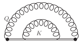
Figure 12: The rainbow diagram

We will label first “rainbow” diagram, shown in Fig. 12, $r$. Its contribution reads

$$\delta\hat{q}_{\scriptscriptstyle L}\Big{|}_{r} = -g^{4}C_{R}\int_{-\infty}^{+\infty}dx^{+}\int_{0}^{x^{+}}dx^{+\prime}\int_{0}^{x^{+\prime}}dx^{+\prime\prime}\int\frac{d^{4}Q}{(2\pi)^{4}}\int\frac{d^{4}K}{(2\pi)^{4}}$$ (134)

$$\times e^{-iq^{-}x^{+}}e^{-ik^{-}(x^{+\prime}-x^{+\prime\prime})}(q^{+})^{2}G^{--}_{rr}(Q)G^{--}_{rr}(K),$$

where, as we remarked in Sec. 6, the specific ordering of the two propagators is not relevant to NLO, as long as they receive a Bose enhancement. The Wilson line integrations yield

$$\delta\hat{q}_{\scriptscriptstyle L}\Big{|}_{r}=g^{4}C_{R}C_{A}\int\frac{d^{4}Q}{(2\pi)^{4}}\int\frac{d^{4}K}{(2\pi)^{4}}\left(\frac{i(q^{+})^{2}}{(q^{-}+i\epsilon)^{2}(q^{-}+k^{-}+i\epsilon)}-\mathrm{adv}\right)G^{--}_{rr}(Q)G^{--}_{rr}(K),$$ (135)

where “adv” stands for the advanced $-i\epsilon\to+i\epsilon$ counterpart of the first term in round brackets. As in Sec. 3.2 and Fig. 7, we set out to perform the $q^{+}$ integration in the complex plane. The integral is very sensitive to large $q^{+}$ due to the $(q^{+})^{2}$ in the numerator; but, contrary to the leading-order case, $q^{-}$ is not fixed to be zero; also, $G_{rr}^{--}(Q)$ contains the statistical function $n_{\scriptscriptstyle B}(q^{0})\simeq T/q^{0}=T/(q^{+}+q^{-}/2)$. Applying some numerator algebra to these terms, we obtain

$$\frac{T(q^{+})^{2}}{q^{+}+q^{-}/2}=Tq^{+}-\frac{Tq^{-}}{2}+\frac{T(q^{-})^{2}}{4(q^{+}+q^{-}/2)}.$$ (136)

The first term yields the contour deformation, the second will vanish as we shall show (no poles and no contour contributions) and the third can be dealt with using Euclidean technology.

We start with the contribution from the first term, with additional label $(a)$ for arc. Upon deforming $q^{+}$ away from the real axis, the retarded propagator turns into Eq. (28), so that

$$\delta\hat{q}_{\scriptscriptstyle L}\Big{|}^{(a)}_{r} = g^{4}C_{R}C_{A}T\int_{\mathcal{C}_{R}}\frac{d^{4}Q}{(2\pi)^{4}}\int\frac{d^{4}K}{(2\pi)^{4}}\left(\frac{i}{(q^{-}+i\epsilon)^{2}(q^{-}+k^{-}+i\epsilon)}-\mathrm{adv}\right)$$ (137)

$$\times G^{--}_{rr}(K)\frac{i}{q^{+}}\left(1+\frac{q^{-}}{q^{+}}\right)\frac{2q^{+}q^{-}-M_{\infty}^{2}}{2q^{+}q^{-}-q_{\perp}^{2}-M_{\infty}^{2}}\Big{|}_{\mathcal{C}_{R}}+\mathcal{C}_{A},$$

where $\mathcal{C}_{R}$ and $\mathcal{C}_{A}$ are the retarded and advanced deformed contours, as defined in Sec. 3.2. The contribution from the latter is not shown explicitly. Let us define $\delta E_{\mathbf{q}}$ and, for later convenience, $\delta E_{\mathbf{q}+\mathbf{k}}$ and $\delta E_{\mathbf{q}-\mathbf{k}}$ as

$$\delta E_{\mathbf{q}}\equiv\frac{q_{\perp}^{2}+M_{\infty}^{2}}{2q^{+}},\qquad\delta E_{\mathbf{q}+\mathbf{k}}\equiv\frac{(\mathbf{q}_{\perp}+\mathbf{k}_{\perp})^{2}+M_{\infty}^{2}}{2q^{+}},\qquad\delta E_{\mathbf{q}-\mathbf{k}}\equiv\frac{(\mathbf{q}_{\perp}-\mathbf{k}_{\perp})^{2}+M_{\infty}^{2}}{2q^{+}}.$$ (138)

When deforming above the $q^{+}$ axis we can then close the $q^{-}$ contour in the lower half-plane, picking the pinched $q^{-}=\delta E_{\mathbf{q}}$ retarded pole (and conversely for the $\mathcal{C}_{A}$ contribution). This yields

$$\delta\hat{q}_{\scriptscriptstyle L}\Big{|}^{(a)}_{r} = -ig^{4}C_{R}C_{A}T\int_{\mathcal{C}_{R}}\frac{dq^{+}d^{2}q_{\perp}}{(2\pi)^{3}}\int\frac{d^{4}K}{(2\pi)^{4}}\left(-\frac{i}{\delta E_{\mathbf{q}}^{2}(\delta E_{\mathbf{q}}+k^{-}-i\epsilon)}\right)$$ (139)

$$\times G^{--}_{rr}(K)\frac{i}{q^{+}}\left(1+\frac{\delta E_{\mathbf{q}}}{q^{+}}\right)\frac{q_{\perp}^{2}}{2q^{+}}+\mathcal{C}_{A}.$$

The final expression, up to order $1/q^{+}$ terms, reads

$$\delta\hat{q}_{\scriptscriptstyle L}\Big{|}^{(a)}_{r}=g^{4}C_{R}C_{A}T\int_{\mathcal{C}_{R}}\frac{dq^{+}}{2\pi}\int\frac{d^{2}q_{\perp}}{(2\pi)^{2}}\int\frac{d^{4}K}{(2\pi)^{4}}\frac{q_{\perp}^{2}G^{--}_{rr}(K)}{2(q^{+})^{2}\delta E_{\mathbf{q}}^{2}}\left(\pi\delta(k^{-})+\frac{i\delta E_{\mathbf{q}}}{(k^{-}-i\epsilon)^{2}}\right)+\mathcal{C}_{A}\,,$$ (140)

where we have used the symmetries of the integrand to express the leading-order term as a $\delta$-function of $k^{-}$.

We now inspect the second term, labeled $(s)$

$$\delta\hat{q}_{\scriptscriptstyle L}\Big{|}^{(s)}_{r}=-\frac{g^{4}C_{R}C_{A}}{2}\int\!\frac{d^{4}Q}{(2\pi)^{4}}\int\!\frac{d^{4}K}{(2\pi)^{4}}\left(\frac{i}{(q^{-}{+}i\epsilon)(q^{-}{+}k^{-}+{i}\epsilon)}-\mathrm{adv}\right)\rho^{--}_{rr}(Q)G^{--}_{rr}(K).$$ (141)

When deforming on $\mathcal{C}_{R}$ and $\mathcal{C}_{A}$ we have

$$\delta\hat{q}_{\scriptscriptstyle L}\Big{|}^{(s)}_{r} = \frac{g^{4}C_{R}C_{A}}{2}\int_{\mathcal{C}_{R}}\frac{dq^{+}}{(2\pi)}\int\frac{dq^{-}d^{2}q_{\perp}}{(2\pi)^{3}}\int\frac{d^{4}K}{(2\pi)^{4}}\left(\frac{i}{(q^{-}-i\epsilon)(q^{-}+k^{-}-i\epsilon)}\right)$$ (142)

$$\times G^{--}_{rr}(K)\frac{i}{(q^{+})^{2}}\left(1+\frac{q^{-}}{q^{+}}\right)\frac{2q^{+}q^{-}-M_{\infty}^{2}}{2q^{+}(q^{-}-\delta E_{\mathbf{q}}+i\epsilon)}+\mathcal{C}_{A}.$$

The $q^{-}$ integration can be performed as before, yielding

$$\delta\hat{q}_{\scriptscriptstyle L}\Big{|}^{(s)}_{r} = -i\frac{g^{4}C_{R}C_{A}}{2}\int_{\mathcal{C}_{R}}\frac{dq^{+}}{(2\pi)}\int\frac{d^{2}q_{\perp}}{(2\pi)^{2}}\int\frac{d^{4}K}{(2\pi)^{4}}\left(\frac{i}{(\delta E_{\mathbf{q}})(\delta E_{\mathbf{q}}+k^{-}-i\epsilon)}\right)$$ (143)

$$\times G^{--}_{rr}(K)\frac{i}{(q^{+})^{2}}\left(1+\frac{q^{-}}{q^{+}}\right)\frac{q_{\perp}^{2}}{2q^{+}}+\mathcal{C}_{A},$$

which goes like $1/(q^{+})^{2}$ and hence is irrelevant. This can be easily understood by noting that the pinched poles in $q^{-}$ force $q^{-}\sim 1/q^{+}$, so that the factor of $q^{-}/q^{+}$ of this term with respect to Eq. (137) behaves like $1/(q^{+})^{2}$.

Finally, we look at the Euclidean term, labeled $(e)$, which reads

$$\delta\hat{q}_{\scriptscriptstyle L}\Big{|}^{(e)}_{r}=g^{4}C_{R}C_{A}\int\frac{d^{4}Q}{(2\pi)^{4}}\int\frac{d^{4}K}{(2\pi)^{4}}2\pi\delta(q^{-}+k^{-})\frac{1}{4}G^{--}_{rr}(Q)G^{--}_{rr}(K).$$ (144)

This term will be canceled by an opposite term in another diagram.

F.2 The crossed rainbow diagram

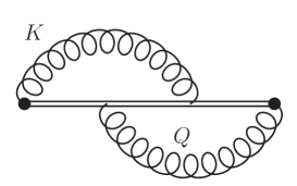
Figure 13: The crossed rainbow diagram

The amplitude of this diagram, shown in Fig. 13 and labeled $+$ for cross, reads

$$\delta\hat{q}_{\scriptscriptstyle L}\Big{|}_{+} = +g^{4}C_{R}C_{A}\int_{-\infty}^{+\infty}dx^{+}\int_{0}^{x^{+}}dx^{+\prime}\int_{0}^{x^{+\prime}}dx^{+\prime\prime}\int\frac{d^{4}Q}{(2\pi)^{4}}\int\frac{d^{4}K}{(2\pi)^{4}}$$ (145)

$$\times e^{-iq^{-}(x^{+}-x^{+\prime\prime})}e^{-ik^{-}x^{+\prime}}q^{+}k^{+}G^{--}_{rr}(Q)G^{--}_{rr}(K).$$

The sign is opposite to Eq. (134) because of the different ordering of the color matrices. Doing the $x^{+}$ integrations we obtain

$$\delta\hat{q}_{\scriptscriptstyle L}\Big{|}_{+} = -g^{4}C_{R}C_{A}\int\frac{d^{4}Q}{(2\pi)^{4}}\int\frac{d^{4}K}{(2\pi)^{4}}\left(\frac{i}{(q^{-}+i\epsilon)(k^{-}+i\epsilon)(q^{-}+k^{-}+i\epsilon)}-\mathrm{adv}\right)$$ (146)

$$\hskip 128.0374pt\times q^{+}k^{+}G^{--}_{rr}(Q)G^{--}_{rr}(K).$$

Again $G^{--}_{rr}(Q)G^{--}_{rr}(K)$ contain statistical functions $\frac{T^{2}}{q^{0}k^{0}}=\frac{4T^{2}}{(2q^{-}+q^{+})(2k^{-}+k^{+})}$. We handle this by performing the following algebra:

$$\frac{4T^{2}q^{+}k^{+}}{(2q^{+}{+}q^{-})(2k^{+}{+}k^{-})}=T^{2}-\frac{T^{2}q^{-}}{2q^{+}{+}q^{-}}-\frac{T^{2}k^{-}}{2k^{+}{+}k^{-}}+\frac{T^{2}q^{-}k^{-}}{(2q^{+}{+}q^{-})(2k^{+}{+}k^{-})}.$$ (147)

The first term will not contribute: deforming the $q^{+}$ integral

$$\delta\hat{q}_{\scriptscriptstyle L}\Big{|}_{+}^{(1)} = g^{4}C_{R}C_{A}T^{2}\int_{\mathcal{C}_{R}}\frac{d^{4}Q}{(2\pi)^{4}}\int\frac{d^{4}K}{(2\pi)^{4}}\left(\frac{i}{(q^{-}-i\epsilon)(k^{-}-i\epsilon)(q^{-}+k^{-}-i\epsilon)}\right)\rho^{--}_{rr}(K)$$ (148)

$$\times\frac{i}{(q^{+})^{2}}\left(1+\frac{q^{-}}{q^{+}}\right)\frac{2q^{+}q^{-}-M_{\infty}^{2}}{2q^{+}(q^{-}-\delta E_{\mathbf{q}}+i\epsilon)}+\mathcal{C}_{A}\,,$$

the $q^{-}$ integration can be closed below, yielding

$$\delta\hat{q}_{\scriptscriptstyle L}\Big{|}_{+}^{(1)} = -ig^{4}C_{R}C_{A}T^{2}\int_{\mathcal{C}_{R}}\frac{dq^{+}d^{2}q_{\perp}}{(2\pi)^{3}}\int\frac{d^{4}K}{(2\pi)^{4}}\left(\frac{i}{\delta E_{\mathbf{q}}(k^{-}-i\epsilon)(k^{-}+\delta E_{\mathbf{q}}-i\epsilon)}\right)\rho^{--}_{rr}(K)$$ (149)

$$\times\frac{i}{(q^{+})^{2}}\left(1+\frac{q^{-}}{q^{+}}\right)\frac{q_{\perp}^{2}}{2q^{+}}+\mathcal{C}_{A}\,.$$

The $k^{-}$ integration can be closed in the upper half-plane, giving

$$\delta\hat{q}_{\scriptscriptstyle L}\Big{|}_{+}^{(1)} = g^{4}C_{R}C_{A}T^{2}\!\int_{\mathcal{C}_{R}}\!\frac{dq^{+}d^{2}q_{\perp}}{(2\pi)^{3}}\int\frac{dk^{+}d^{2}k_{\perp}}{(2\pi)^{3}}\frac{i}{\delta E_{\mathbf{q}}^{2}}\left[G_{R}^{--}(k^{-}{=}0)-G_{R}^{--}(k^{-}{=}-\delta E_{\mathbf{q}})\right]$$ (150)

$$\times\frac{i}{(q^{+})^{2}}\left(1+\frac{q^{-}}{q^{+}}\right)\frac{q_{\perp}^{2}}{2q^{+}}+\mathcal{C}_{A}\,.$$

This vanishes on $\mathcal{C}_{R}$, because the square bracket is at least linear in $\delta E_{\mathbf{q}}$.

The second and third term are identical to Eq. (141) and thus vanish. Only the last term contributes, yielding

$$\delta\hat{q}_{\scriptscriptstyle L}\Big{|}_{+}=-g^{4}C_{R}C_{A}\int\frac{d^{4}Q}{(2\pi)^{4}}\int\frac{d^{4}K}{(2\pi)^{4}}\frac{2\pi\delta(q^{-}+k^{-})}{4}G^{--}_{rr}(Q)G^{--}_{rr}(K),$$ (151)

which cancels Eq. (144).

F.3 The cat eye diagram

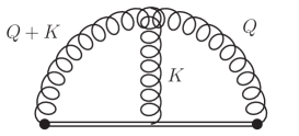
Figure 14: The cat-eye diagram

The diagram is shown in Fig. 14, and will be labeled $c$ for cat-eye. Using only the bare vertex, the graph yields

$$\delta\hat{q}_{\scriptscriptstyle L}\Big{|}_{c}\!\! = g^{4}C_{R}C_{A}\!\int_{-\infty}^{+\infty}\!\!dx^{+}\!\int_{0}^{x^{+}}\!\!\!dx^{+\prime}\int\!\frac{d^{4}Q}{(2\pi)^{4}}\int\!\frac{d^{4}K}{(2\pi)^{4}}e^{-i(q^{-}x^{+}+k^{-}x^{+\prime})}\Gamma_{\mu\nu\rho}(-Q,-K,Q{+}K)$$ (152)

$$\times q^{+}(q^{+}+k^{+})\bigg{[}G_{A}^{-\rho}(Q{+}K)G_{rr}^{-\nu}(K)G_{rr}^{-\mu}(Q)+G_{rr}^{-\rho}(Q{+}K)G_{R}^{-\nu}(K)G_{rr}^{-\mu}(Q)$$

$$+G_{rr}^{-\rho}(Q{+}K)G_{rr}^{-\nu}(K)G_{R}^{-\mu}(Q)\bigg{]},$$

where we have defined the three-gluon vertex as

$$gf^{abc}\Gamma^{\mu\nu\rho}(P,Q,K)\equiv-gf^{abc}\left[g^{\mu\nu}(P-Q)^{\rho}+g^{\nu\rho}(Q-K)^{\mu}+g^{\rho\mu}(K-P)^{\nu}\right].$$ (153)

$P,Q,K$ are all inflowing in the vertex, $P$ is associated with $a$ and $\mu$ and similarly for the others. The $x^{+}$ and $x^{+\prime}$ integrals yield

$$\delta\hat{q}_{\scriptscriptstyle L}\Big{|}_{c}\!\! = g^{4}C_{R}C_{A}\!\int\!\frac{d^{4}Q}{(2\pi)^{4}}\!\int\!\frac{d^{4}K}{(2\pi)^{4}}\!\left(\frac{1}{(q^{-}{+}i\epsilon)(q^{-}{+}k^{-}{+}i\epsilon)}-\mathrm{adv}\right)\Gamma_{\mu\nu\rho}(-Q,-K,Q{+}K)$$ (154)

$$\times q^{+}(q^{+}+k^{+})\bigg{[}G_{A}^{-\rho}(Q{+}K)G_{rr}^{-\nu}(K)G_{rr}^{-\mu}(Q)+G_{rr}^{-\rho}(Q{+}K)G_{R}^{-\nu}(K)G_{rr}^{-\mu}(Q)$$

$$+G_{rr}^{-\rho}(Q{+}K)G_{rr}^{-\nu}(K)G_{R}^{-\mu}(Q)\bigg{]}.$$

Let us look at the $r/a$ structure of the propagators. Suppressing Lorentz indices and using $G_{rr}(K)=n_{\scriptscriptstyle B}(K)(G_{R}(K)-G_{A}(K))$, $n_{\scriptscriptstyle B}(K)\simeq T/k^{0}$, the last two lines can be rewritten as

$$Tq^{+}G_{rr}(K)\big{[}G_{R}(Q)G_{R}(Q{+}K)-G_{A}(Q)G_{A}(Q{+}K)\big{]}$$

$$+T^{2}\rho(Q)\big{[}G_{R}(K)G_{R}(Q{+}K)-G_{A}(K)G_{A}(Q{+}K)\big{]}$$

$$-T\frac{q^{-}}{2}G_{rr}(Q)\big{[}\rho(K)G_{A}(Q{+}K)+\rho(Q{+}K)G_{R}(K)\big{]}$$

$$-T\frac{q^{-}+k^{-}}{2}G_{rr}(K)\big{[}\rho(Q)G_{A}(Q{+}K)+\rho(Q{+}K)G_{R}(Q)\big{]}$$

$$-T\frac{q^{-}+k^{-}}{2}G_{rr}(Q{+}K)\big{[}\rho(Q)G_{R}(K)-\rho(K)G_{R}(Q)\big{]}$$

$$+\frac{q^{-}(q^{-}+k^{-})}{4}\bigg{\{}G_{rr}(Q)\big{[}G_{rr}(K)G_{A}(Q{+}K)+G_{R}(K)G_{rr}(Q{+}K)\big{]}$$

$$+G_{rr}(K)G_{rr}(Q{+}K)G_{R}(Q)\bigg{\}}.$$ (155)

We start by dealing with the first line, which has the highest power of $q^{+}$ in the numerator. We label its contribution $(1)$. It reads

$$\delta\hat{q}_{\scriptscriptstyle L}\Big{|}_{c}^{(1)} = g^{4}C_{R}C_{A}\int\frac{d^{4}Q}{(2\pi)^{4}}\int\frac{d^{4}K}{(2\pi)^{4}}\left(\frac{1}{(q^{-}+i\epsilon)(q^{-}+k^{-}+i\epsilon)}-\mathrm{adv}\right)Tq^{+}G_{rr}^{-\nu}(K)$$

$$\times\Gamma_{\mu\nu\rho}(-Q,-K,Q{+}K)\bigg{[}G_{R}^{-\mu}(Q)G_{R}^{-\rho}(Q{+}K)-G_{A}^{-\mu}(Q)G_{A}^{-\rho}(Q{+}K)\bigg{]}.$$

Having obtained a fully retarded (advanced) function of $q^{+}$ we can now expand on $\mathcal{C}_{R}$ ($\mathcal{C}_{A}$). Similar comments about pinching poles apply here as well: we expect $G_{R}^{T}(Q)$ and $G_{R}^{T}(Q{+}K)$ to introduce poles for $q^{-}=\delta E_{\mathbf{q}}$ and $q^{-}+k^{-}=\delta E_{\mathbf{q}+\mathbf{k}}$ respectively. Indeed we obtain

$$\delta\hat{q}_{\scriptscriptstyle L}\Big{|}_{c}^{(1)} = g^{4}C_{R}C_{A}T\int_{\mathcal{C}_{R}}\frac{dq^{+}}{2\pi}\int\frac{dq^{-}d^{2}q_{\perp}}{(2\pi)^{3}}\int\frac{d^{4}K}{(2\pi)^{4}}\left(\frac{1}{(q^{-}+i\epsilon)(q^{-}+k^{-}+i\epsilon)}-\mathrm{adv}\right)$$

$$\times\bigg{[}2(q_{\perp}^{2}+\mathbf{q}_{\perp}\cdot\mathbf{k}_{\perp})G^{T}_{R}(Q)G^{T}_{R}(Q{+}K)G_{rr}^{--}(K)+\mathcal{O}\left(\frac{1}{q^{+}}\right)\bigg{]}+\mathcal{C}_{A}.$$

Expanding the transverse propagators to order $1/(q^{+})^{2}$ we have

$$G^{T}_{R}(Q)\to \frac{i}{2q^{+}(q^{-}-\delta E_{\mathbf{q}}+i\epsilon)},$$

$$\qquad G^{T}_{R}(Q{+}K)\to \frac{i}{2q^{+}(q^{-}{+}k^{-}{-}\delta E_{\mathbf{q}+\mathbf{k}}{+}i\epsilon)}\left(1-\frac{q^{-}+k^{-}}{q^{+}(q^{-}{+}k^{-}{-}\delta E_{\mathbf{q}+\mathbf{k}}{+}i\epsilon)}\right),$$ (158)

and considering only the $(1/q^{+})^{0}$ terms in Eq. (LABEL:catexpanded) we have

$$\delta\hat{q}_{\scriptscriptstyle L}\Big{|}_{c}^{(1)} = -g^{4}C_{R}C_{A}T\int_{\mathcal{C}_{R}}\frac{dq^{+}}{2\pi}\int\frac{dq^{-}d^{2}q_{\perp}}{(2\pi)^{3}}\int\frac{d^{4}K}{(2\pi)^{4}}\left(\frac{1}{(q^{-}+i\epsilon)(q^{-}+k^{-}+i\epsilon)}-\mathrm{adv}\right)$$ (159)

$$\times\bigg{[}\frac{(q_{\perp}^{2}+\mathbf{q}_{\perp}\cdot\mathbf{k}_{\perp})G_{rr}^{--}(K)}{2(q^{+})^{2}(q^{-}{-}\delta E_{\mathbf{q}}+i\epsilon)(q^{-}{+}k^{-}{-}\delta E_{\mathbf{q}+\mathbf{k}}+i\epsilon)}\left(1-\frac{q^{-}+k^{-}}{q^{+}(q^{-}{+}k^{-}{-}\delta E_{\mathbf{q}+\mathbf{k}}{+}i\epsilon)}\right)\bigg{]}$$

$$+\mathcal{C}_{A}.$$

Rewriting the terms in round brackets as $\delta$-functions gives

$$\delta\hat{q}_{\scriptscriptstyle L}\Big{|}^{(1)}_{ca} = -ig^{4}C_{R}C_{A}T\int_{\mathcal{C}_{R}}\frac{dq^{+}}{2\pi}\int\frac{dq^{-}d^{2}q_{\perp}}{(2\pi)^{3}}\int\frac{d^{4}K}{(2\pi)^{4}}2\pi P\frac{1}{k^{-}}\left(\delta(q^{-}+k^{-})-\delta(q^{-})\right)$$ (160)

$$\times\bigg{[}\frac{(q_{\perp}^{2}+\mathbf{q}_{\perp}\cdot\mathbf{k}_{\perp})G_{rr}^{--}(K)}{2(q^{+})^{2}(q^{-}{-}\delta E_{\mathbf{q}}+i\epsilon)(q^{-}{+}k^{-}{-}\delta E_{\mathbf{q}+\mathbf{k}}+i\epsilon)}\left(1-\frac{q^{-}+k^{-}}{q^{+}(q^{-}{+}k^{-}{-}\delta E_{\mathbf{q}+\mathbf{k}}{+}i\epsilon)}\right)\bigg{]}$$

$$+\mathcal{C}_{A}.$$

where $P$ denotes the principal value. This yields

$$\delta\hat{q}_{\scriptscriptstyle L}\Big{|}^{(1)}_{ca} = -ig^{4}C_{R}C_{A}T\int_{\mathcal{C}_{R}}\frac{dq^{+}}{2\pi}\int\frac{d^{2}q_{\perp}}{(2\pi)^{2}}\int\frac{d^{4}K}{(2\pi)^{4}}\frac{(q_{\perp}^{2}+\mathbf{q}_{\perp}\cdot\mathbf{k}_{\perp})G_{rr}^{--}(K)}{2(q^{+})^{2}}$$ (161)

$$\times P\frac{1}{k^{-}}\bigg{[}\frac{1}{\delta E_{\mathbf{q}}(k^{-}-\delta E_{\mathbf{q}+\mathbf{k}}+i\epsilon)}\left(1-\frac{k^{-}}{q^{+}(k^{-}{-}\delta E_{\mathbf{q}+\mathbf{k}}{+}i\epsilon)}\right)$$

$$+\frac{1}{(k^{-}+\delta E_{\mathbf{q}}-i\epsilon)\delta E_{\mathbf{q}+\mathbf{k}}}\bigg{]}+\mathcal{C}_{A}.$$

With some algebra and making pinches explicit we have

$$\delta\hat{q}_{\scriptscriptstyle L}\Big{|}^{(1)}_{ca} = -ig^{4}C_{R}C_{A}T\int_{\mathcal{C}_{R}}\frac{dq^{+}}{2\pi}\int\frac{d^{2}q_{\perp}}{(2\pi)^{2}}\int\frac{d^{4}K}{(2\pi)^{4}}\frac{(q_{\perp}^{2}+\mathbf{q}_{\perp}\cdot\mathbf{k}_{\perp})G_{rr}^{--}(K)}{4(q^{+})^{2}}$$ (162)

$$\times\bigg{[}\frac{1}{\delta E_{\mathbf{q}}(k^{-}-\delta E_{\mathbf{q}+\mathbf{k}}+i\epsilon)}\left(1-\frac{k^{-}}{q^{+}(k^{-}{-}\delta E_{\mathbf{q}+\mathbf{k}}{+}i\epsilon)}\right)\left(\frac{2}{k^{-}+i\epsilon}+2\pi i\delta(k^{-})\right)$$

$$+\frac{1}{(k^{-}+\delta E_{\mathbf{q}}-i\epsilon)\delta E_{\mathbf{q}+\mathbf{k}}}\left(\frac{2}{k^{-}-i\epsilon}-2\pi i\delta(k^{-})\right)\bigg{]}+\mathcal{C}_{A},$$

which gives, upon expanding the non-pinched denominators

$$\delta\hat{q}_{\scriptscriptstyle L}\Big{|}^{(1)}_{ca} = -ig^{4}C_{R}C_{A}T\int_{\mathcal{C}_{R}}\frac{dq^{+}}{2\pi}\int\frac{d^{2}q_{\perp}}{(2\pi)^{2}}\int\frac{d^{4}K}{(2\pi)^{4}}\frac{(q_{\perp}^{2}+\mathbf{q}_{\perp}\cdot\mathbf{k}_{\perp})G_{rr}^{--}(K)}{2(q^{+})^{2}\delta E_{\mathbf{q}}\delta E_{\mathbf{q}+\mathbf{k}}}$$ (163)

$$\times\bigg{[}-2\pi i\delta(k^{-})+\frac{\delta E_{\mathbf{q}+\mathbf{k}}}{(k^{-}+i\epsilon)^{2}}+\frac{\delta E_{\mathbf{q}}}{(k^{-}-i\epsilon)^{2}}\bigg{]}+\mathcal{C}_{A}.$$

We have dropped terms that are $\mathcal{O}(1/(q^{+})^{2})$. The terms suppressed by one further power of $1/q^{+}$ in Eq. (LABEL:catexpanded) turn out to be either completely independent of $q^{-}$ on $\mathcal{C}_{R}$, and hence vanishing when its integration is done, or proportional to the terms in Eq. (159) times $k^{-}/q^{+}$, $q^{-}/q^{+}$ or $k^{+}/q^{+}$. From the previous calculation it should be clear that the only way they could contribute at order $1/q^{+}$ on $\mathcal{C}_{R}$ would be if both pinches ($q^{-}$ and $q^{-}+k^{-}$) were taken. In the first two cases that is not possible, because the factors of $q^{-}$ or $k^{-}$ at the numerator eliminate either of the two pinched poles and in the last case the resulting $k^{+}$ integration is odd once $k^{-}$ is set to zero.

We now consider the second line in Eq. (155), which we label $(2)$:

$$\delta\hat{q}_{\scriptscriptstyle L}\Big{|}_{c}^{(2)}\!\! = \!g^{4}C_{R}C_{A}\!\int\!\frac{d^{4}Q}{(2\pi)^{4}}\!\int\!\frac{d^{4}K}{(2\pi)^{4}}\left(\frac{1}{(q^{-}{+}i\epsilon)(q^{-}{+}k^{-}{+}i\epsilon)}-\mathrm{adv}\right)T^{2}\rho^{-\mu}(Q)$$

$$\times\Gamma_{\mu\nu\rho}(-Q,-K,Q{+}K)\bigg{[}G_{R}^{-\nu}(K)G_{R}^{-\rho}(Q{+}K)-G_{A}^{-\nu}(K)G_{A}^{-\rho}(Q{+}K)\bigg{]}.$$

We can now deform the $k^{+}$ integration, obtaining

$$\delta\hat{q}_{\scriptscriptstyle L}\Big{|}_{c}^{(2)} = -g^{4}C_{R}C_{A}T^{2}\int_{\mathcal{C}_{R}}\frac{dk^{+}dk^{-}d^{2}k_{\perp}}{(2\pi)^{4}}\int\frac{d^{4}Q}{(2\pi)^{4}}\left(\frac{1}{(q^{-}+i\epsilon)(q^{-}+k^{-}+i\epsilon)}-\mathrm{adv}\right)$$ (165)

$$\times\frac{2(k_{\perp}^{2}+\mathbf{k}_{\perp}\cdot\mathbf{q}_{\perp})G^{T}_{R}(K)G^{T}_{R}(Q{+}K)\rho^{--}(Q)}{k^{+}},$$

which is very similar to what we had before, due to the symmetries of the vertex. Higher-order terms in the expansion will not be relevant, as this contribution is one power smaller on the arc. Hence, replacing the transverse propagators with their leading-order expressions (158) and rewriting the terms in round brackets as $\delta$-functions we have

$$\delta\hat{q}_{\scriptscriptstyle L}\Big{|}_{c}^{(2)} = +ig^{4}C_{R}C_{A}T^{2}\int_{\mathcal{C}_{R}}\frac{dk^{+}dk^{-}d^{2}k_{\perp}}{(2\pi)^{4}}\int\frac{d^{4}Q}{(2\pi)^{4}}2\pi P\frac{1}{k^{-}}(\delta(q^{-}+k^{-})-\delta(q^{-}))$$ (166)

$$\times\frac{(k_{\perp}^{2}+\mathbf{k}_{\perp}\cdot\mathbf{q}_{\perp})\rho^{--}(Q)}{2(k^{+})^{3}(k^{-}-\delta E_{\mathbf{q}}+i\epsilon)(k^{-}+q^{-}-\delta E_{\mathbf{q}+\mathbf{k}}+i\epsilon)},$$

which yields

$$\delta\hat{q}_{\scriptscriptstyle L}\Big{|}_{c}^{(2)} = -ig^{4}C_{R}C_{A}T^{2}\int_{\mathcal{C}_{R}}\frac{dk^{+}dk^{-}d^{2}k_{\perp}}{(2\pi)^{4}}\int\frac{dq^{+}d^{2}q_{\perp}}{(2\pi)^{3}}P\frac{1}{k^{-}}\frac{(k_{\perp}^{2}+\mathbf{k}_{\perp}\cdot\mathbf{q}_{\perp})}{2(k^{+})^{3}}$$ (167)

$$\times\bigg{[}\frac{\rho^{--}(-k^{-},q^{+},q_{\perp})}{(k^{-}-\delta E_{\mathbf{q}}+i\epsilon)\delta E_{\mathbf{q}+\mathbf{k}}}+\frac{\rho^{--}(0,q^{+},q_{\perp})}{(k^{-}-\delta E_{\mathbf{q}}+i\epsilon)(k^{-}-\delta E_{\mathbf{q}+\mathbf{k}}+i\epsilon)}\bigg{]}.$$

The second term on the bottom line vanishes under the $q^{+}$ integration, as it is odd. Similarly, the first term yields

$$\delta\hat{q}_{\scriptscriptstyle L}\Big{|}_{c}^{(2)} = -g^{4}C_{R}C_{A}T^{2}\int_{\mathcal{C}_{R}}\frac{dk^{+}d^{2}k_{\perp}}{(2\pi)^{3}}\int\frac{dq^{+}d^{2}q_{\perp}}{(2\pi)^{3}}\frac{(k_{\perp}^{2}+\mathbf{k}_{\perp}\cdot\mathbf{q}_{\perp})}{2(k^{+})^{3}\delta E_{\mathbf{q}+\mathbf{k}}\delta E_{\mathbf{q}}}$$ (168)

$$\times\bigg{[}G^{--}_{R}(-\delta E_{\mathbf{q}},q^{+},q_{\perp})-G_{R}^{--}(0,q^{+},q_{\perp})\bigg{]},$$

which vanishes, as the $q^{+}$ integration can only pick up the residue of the Coulomb gauge poles, which is $\mathcal{O}(\delta E_{\mathbf{q}})$ and thus makes the $k^{+}$ integration vanish.

Finally, terms with $q^{-}$ or $q^{-}+k^{-}$ at the numerator in Eq. (155) vanish again for the loss of $q^{+}$ at the numerator and of a pinched pole at the denominator. The last term trivially vanishes. The entire result is hence given by Eq. (163).

F.4 Self-energy diagrams

We analyze separately the two diagrams show in Fig. 15, the loop diagram on the left and the tadpole diagram on the right.

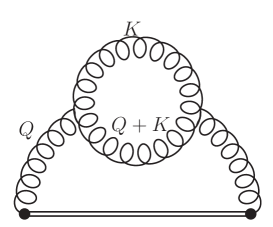
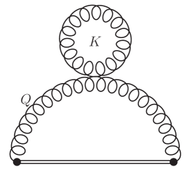
Figure 15: The loop diagram on the left and the tadpole diagram on the right.

F.4.1 The loop diagram

The amplitude is labeled by $l$ and reads

$$\delta\hat{q}_{\scriptscriptstyle L}\Big{|}_{\mathrm{l}} = \frac{g^{4}C_{R}C_{A}}{2}\int\frac{dq^{+}d^{2}q_{\perp}}{(2\pi)^{3}}\int\frac{d^{4}K}{(2\pi)^{4}}Tq^{+}\Gamma_{\mu\nu\rho}(Q,-Q-K,K)\Gamma_{\mu^{\prime}\nu^{\prime}\rho^{\prime}}(-Q,Q{+}K,-K)$$

$$\times\bigg{\{}G^{-\mu}_{R}(Q)G^{-\mu^{\prime}}_{R}(Q)\big{[}G_{rr}^{\nu\nu^{\prime}}(Q{+}K)G_{A}^{\rho\rho^{\prime}}(K)+G_{R}^{\nu\nu^{\prime}}(Q{+}K)G_{rr}^{\rho\rho^{\prime}}(K)\big{]}-\mathrm{adv}\bigg{\}}_{q^{-}=0},$$

where $1/2$ is a symmetry factor. We now perform a shift $K\to K-Q$ in the first term in square brackets on the second line. In principle one should be careful in performing such operations, as the integrals here are not finite. Indeed, as we anticipated, we will need to subtract the HTL counterterm, which, however, is obtained by performing the same shift, as we will show in Sec. F.5. We then have

$$\delta\hat{q}_{\scriptscriptstyle L}\Big{|}_{\mathrm{l}} = \frac{g^{4}C_{R}C_{A}}{2}\int\frac{dq^{+}d^{2}q_{\perp}}{(2\pi)^{3}}\int\frac{d^{4}K}{(2\pi)^{4}}Tq^{+}\bigg{\{}G^{-\mu}_{R}(Q)G^{-\mu^{\prime}}_{R}(Q)$$

$$\times\bigg{[}\Gamma_{\mu\nu\rho}(Q,-Q-K,K)\Gamma_{\mu^{\prime}\nu^{\prime}\rho^{\prime}}(-Q,Q{+}K,-K)G_{R}^{\nu\nu^{\prime}}(Q{+}K)G_{rr}^{\rho\rho^{\prime}}(K)$$

$$+\Gamma_{\mu\nu\rho}(Q,-K,K-Q)\Gamma_{\mu^{\prime}\nu^{\prime}\rho^{\prime}}(-Q,K,-K+Q)G_{rr}^{\nu\nu^{\prime}}(K)G_{A}^{\rho\rho^{\prime}}(K-Q)\bigg{]}-\mathrm{adv}\bigg{\}}_{q^{-}=0}.$$

We are now free to deform the contour, since in this case there are no statistical factor poles, as $q^{-}$ is set to zero. We then have

$$\delta\hat{q}_{\scriptscriptstyle L}\Big{|}_{\mathrm{l}} = g^{4}C_{R}C_{A}\int_{\mathcal{C}_{R}}\frac{dq^{+}}{2\pi}\int\frac{d^{2}q_{\perp}}{(2\pi)^{2}}\int\frac{d^{4}K}{(2\pi)^{4}}\frac{2Tq^{+}q_{\perp}^{2}}{(q_{\perp}^{2}+M_{\infty}^{2})^{2}}\bigg{[}\left(G_{R}^{T}(K+Q)+G^{T}_{A}(K-Q)\right)$$ (171)

$$\times G_{++}^{rr}(K)-\frac{(k^{-}+2k^{+})}{2q^{+}}\left(G^{T}_{A}(K-Q)-G_{R}^{T}(K+Q)\right)G_{L}^{rr}(K)$$

$$+i\frac{G_{T}^{rr}(K)}{(q^{+})^{2}}\left(\frac{1}{2}-\frac{(\mathbf{q}_{\perp}\cdot\mathbf{k}_{\perp})^{2}}{2q_{\perp}^{2}k^{2}}\right)+\mathcal{O}\left(1/(q^{+})^{2}\right)\bigg{]}_{q^{-}=0}+\mathcal{C}_{A}.$$

Terms that had a linear term in the azimuthal angle at the numerator have been neglected. Since there are no pinching poles in $k^{-}$ we can safely expand the $K\pm Q$ propagators, yielding for their sum, up to order $1/(q^{+})^{2}$

$$G_{R}^{T}(K+Q)+G^{T}_{A}(K-Q)=\frac{\pi\delta(k^{-})}{q^{+}}+\frac{i}{2q^{+}}\left[\frac{\delta E_{\mathbf{q}+\mathbf{k}}}{(k^{-}+i\epsilon)^{2}}+\frac{\delta E_{\mathbf{q}-\mathbf{k}}}{(k^{-}-i\epsilon)^{2}}-\frac{2k^{+}}{q^{+}}P\frac{1}{k^{-}}\right],$$ (172)

whereas the difference is

$$G_{A}^{T}(K-Q)-G^{T}_{R}(K+Q)=-\frac{i}{q^{+}}P\frac{1}{k^{-}}+\mathcal{O}\left(\frac{1}{(q^{+})^{2}}\right).$$ (173)

Plugging this back in Eq. (171) we obtain

$$\delta\hat{q}_{\scriptscriptstyle L}\Big{|}_{\mathrm{l}} = 2g^{4}C_{R}C_{A}T\int_{\mathcal{C}_{R}}\frac{dq^{+}}{2\pi}\int\frac{d^{2}q_{\perp}}{(2\pi)^{2}}\int\frac{d^{4}K}{(2\pi)^{4}}\frac{q_{\perp}^{2}}{(q_{\perp}^{2}+M_{\infty}^{2})^{2}}\bigg{\{}G_{++}^{rr}(K)\bigg{[}\pi\delta(k^{-})$$ (174)

$$\left.+\frac{i}{2}\left(\frac{\delta E_{\mathbf{q}+\mathbf{k}}}{(k^{-}+i\epsilon)^{2}}+\frac{\delta E_{\mathbf{q}-\mathbf{k}}}{(k^{-}-i\epsilon)^{2}}-\frac{2k^{+}}{q^{+}}P\frac{1}{k^{-}}\right)\right]+\frac{i(k^{-}+2k^{+})}{2q^{+}}G_{L}^{rr}(K)P\frac{1}{k^{-}}$$

$$+i\frac{G_{T}^{rr}(K)}{q^{+}}\left(\frac{1}{2}-\frac{(\mathbf{q}_{\perp}\cdot\mathbf{k}_{\perp})^{2}}{2q_{\perp}^{2}k^{2}}\right)+\mathcal{O}\left(1/(q^{+})^{2}\right)\bigg{\}}+\mathcal{C}_{A}.$$

F.4.2 The tadpole diagram

The amplitude, labeled by $t$, reads

$$\delta\hat{q}_{\scriptscriptstyle L}\Big{|}_{\mathrm{t}} = \frac{-ig^{4}C_{R}C_{A}}{2}\int\frac{dq^{+}d^{2}q_{\perp}}{(2\pi)^{3}}\int\frac{d^{4}K}{(2\pi)^{4}}Tq^{+}\bigg{[}G^{-\mu}_{R}(Q)G^{-\nu}_{R}(Q)G_{rr}^{\rho\sigma}(K)$$ (175)

$$\times\left(2g_{\mu\nu}g_{\rho\sigma}-g_{\mu\rho}g_{\nu\sigma}-g_{\mu\sigma}g_{\nu\rho}\right)-\mathrm{adv}\bigg{]}_{q^{-}=0}.$$

Expanding on $\mathcal{C}_{R}$ we have

$$\delta\hat{q}_{\scriptscriptstyle L}\Big{|}_{\mathrm{t}} = \frac{-ig^{4}C_{R}C_{A}T}{2}\int_{\mathcal{C}_{R}}\frac{dq^{+}}{2\pi}\int\frac{d^{2}q_{\perp}}{(2\pi)^{2}}\int\frac{d^{4}K}{(2\pi)^{4}}\frac{2}{q^{+}(q_{\perp}^{2}+M_{\infty}^{2})^{2}}\bigg{[}q_{\perp}^{2}G_{L}^{rr}(K)$$ (176)

$$\left.-\left(q_{\perp}^{2}+\frac{(\mathbf{q}_{\perp}\cdot\mathbf{k}_{\perp})^{2}}{k^{2}}\right)G_{T}^{rr}(K)+\mathcal{O}\left(\frac{1}{(q^{+})^{2}}\right)\right]+\mathcal{C}_{A}.$$

F.4.3 Summary

Summing Eqs. (174), (176) we obtain

$$\delta\hat{q}_{\scriptscriptstyle L}\Big{|}_{\mathrm{t+l-ct}} = g^{4}C_{R}C_{A}T\int_{\mathcal{C}_{R}}\frac{dq^{+}}{2\pi}\int\frac{d^{2}q_{\perp}}{(2\pi)^{2}}\int\frac{d^{4}K}{(2\pi)^{4}}\frac{q_{\perp}^{2}}{4(q^{+})^{2}\delta E_{\mathbf{q}}^{2}}\bigg{\{}G_{++}^{rr}(K)2\pi\delta(k^{-})$$ (177)

$$+\frac{2i\delta E_{\mathbf{q}}G_{++}^{rr}(K)}{(k^{-}-i\epsilon)^{2}}+\frac{i}{q^{+}}\bigg{[}\frac{k_{\perp}^{2}G_{rr}^{--}(K)}{(k^{-}-i\epsilon)^{2}}+G_{T}^{rr}(K)\bigg{(}2-\frac{2k^{+}k_{\perp}^{2}}{k^{2}(k^{-}-i\epsilon)}\bigg{)}\bigg{]}\bigg{\}}$$

$$+\mathcal{C}_{A},$$

where we have used the fact that $\delta E_{\mathbf{q}\pm\mathbf{k}}=\delta E_{\mathbf{q}}+k_{\perp}^{2}/(2q^{+})$, up to vanishing terms in the azimuthal integration and that the square bracket on the second line, which can be identified with the NLO contribution to $Z_{g}$ in Coulomb gauge CaronHuot:2008uw ; Ghiglieri:2013gia , is purely real, so that the prescription used for the $k^{-}$ poles at the denominator there is irrelevant.

F.5 The subtraction term

We now turn to the computation of the subtraction counterterm $\delta\hat{q}_{\scriptscriptstyle L}\Big{|}^{\mathrm{diff}}_{\mathrm{subtr.}}$, i.e. the soft part of the HTL self-energy. To this end, we need only the gluon loop, as soft fermions are not Bose enhanced and do not contribute to relative $\mathcal{O}(g)$. The contribution from the loop diagram is, after the previously-discussed shift

$$\delta\hat{q}_{\scriptscriptstyle L}\Big{|}_{\mathrm{l\,subtr.}}^{\mathrm{diff}} = \frac{g^{4}C_{R}C_{A}}{2}\int\frac{d^{4}Q}{(2\pi)^{4}}\int\frac{d^{4}K}{(2\pi)^{4}}Tq^{+}\Gamma_{\mu\nu\rho}(0,-K,K)\Gamma_{\mu^{\prime}\nu^{\prime}\rho^{\prime}}(0,K,-K)2\pi\delta(q^{-})$$

$$\times\bigg{\{}G^{-\mu}_{R}(Q)G^{-\mu^{\prime}}_{R}(Q)\bigg{[}G_{R}^{(0)\,\nu\nu^{\prime}}(Q{+}K)G_{rr}^{(0)\,\rho\rho^{\prime}}(K)+G_{rr}^{(0)\,\nu\nu^{\prime}}(K)G_{A}^{(0)\,\rho\rho^{\prime}}(K{-}Q)\bigg{]}-\mathrm{adv}\bigg{\}},$$

where the vertices are treated in the HTL approximation, i.e. $Q\ll K$, and the $G^{(0)}$ propagators on the second line are bare and in the soft approximation, $n_{\scriptscriptstyle B}(k^{0})\to T/k^{0}$. This yields

$$\delta\hat{q}_{\scriptscriptstyle L}\Big{|}_{\mathrm{l\,subtr.}}^{\mathrm{diff}}\!\!=ig^{4}C_{R}C_{A}T\!\int_{\mathcal{C}_{R}}\!\!\frac{dq^{+}d^{2}q_{\perp}}{(2\pi)^{3}q^{+}}\!\int\!\!\frac{d^{4}K}{(2\pi)^{4}}\frac{G_{rr}^{(0)\,T}(K)}{(q_{\perp}^{2}+M_{\infty}^{2})^{2}}\bigg{[}q_{\perp}^{2}-\frac{(\mathbf{q}_{\perp}\cdot\mathbf{k}_{\perp})^{2}}{k^{2}}\bigg{]}+\mathcal{C}_{A},$$ (179)

where we have used the fact that in Coulomb gauge the bare longitudinal spectral density vanishes and the transverse one puts $K$ on shell. Furthermore, consistently with the HTL approximation, in $G^{(0)\rho\rho^{\prime}}(K\pm Q)$ one has only to keep the leading terms in $K\gg Q$, i.e. $(Q\pm K)^{2}\to\pm 2Q\cdot K$, $(\mathbf{q}\pm\mathbf{k})^{2}\to k^{2}$. Other terms in the propagators and vertices do not contribute, as discussed in Ghiglieri:2013gia .

The tadpole contribution is trivially obtained from Eq. (176) by replacing the resummed $K$ propagator with its bare counterpart, i.e.

$$\delta\hat{q}_{\scriptscriptstyle L}\Big{|}_{\mathrm{t\,subtr.}}^{\mathrm{diff}}\!\!=ig^{4}C_{R}C_{A}T\!\int_{\mathcal{C}_{R}}\!\frac{dq^{+}d^{2}q_{\perp}}{(2\pi)^{3}q^{+}}\!\int\!\frac{d^{4}K}{(2\pi)^{4}}\frac{G^{(0)\,T}_{rr}(K)}{(q_{\perp}^{2}{+}M_{\infty}^{2})^{2}}\bigg{[}q_{\perp}^{2}+\frac{(\mathbf{q}_{\perp}\cdot\mathbf{k}_{\perp})^{2}}{k^{2}}\bigg{]}+\mathcal{C}_{A},$$ (180)

so that the sum is

$$\delta\hat{q}_{\scriptscriptstyle L}\Big{|}_{\mathrm{subtr.}}^{\mathrm{diff}}=ig^{4}C_{R}C_{A}T\int_{\mathcal{C}_{R}}\frac{dq^{+}d^{2}q_{\perp}}{(2\pi)^{3}}\int\frac{d^{4}K}{(2\pi)^{4}}\frac{2q_{\perp}^{2}G_{rr}^{(0)\,T}(K)}{q^{+}(q_{\perp}^{2}+M_{\infty}^{2})^{2}}+\mathcal{C}_{A}.$$ (181)

F.6 Summary

Summing the contributions from all diagrams and subtracting the counterterm (181) we obtain

$$\delta\hat{q}_{\scriptscriptstyle L}\Big{|}_{\mathrm{loop}}\!\!\!-\delta\hat{q}_{\scriptscriptstyle L}\Big{|}_{\mathrm{subtr.}}^{\mathrm{diff}}\!\! = g^{4}C_{R}C_{A}T\!\int_{\mathcal{C}_{R}}\!\frac{dq^{+}}{2\pi}\!\int\!\frac{d^{2}q_{\perp}}{(2\pi)^{2}}\!\int\!\frac{d^{4}K}{(2\pi)^{4}}$$

$$\times\bigg{\{}\frac{G^{--}_{rr}(K)\pi\delta(k^{-})}{(q^{+})^{2}\delta E_{\mathbf{q}}}\left(\frac{q_{\perp}^{2}}{\delta E_{\mathbf{q}}}-\frac{(q_{\perp}^{2}+\mathbf{q}_{\perp}\cdot\mathbf{k}_{\perp})}{\delta E_{\mathbf{q}+\mathbf{k}}}\right)$$

$$+\frac{iq_{\perp}^{2}}{4(q^{+})^{3}\delta E_{\mathbf{q}}^{2}}\bigg{[}\frac{k_{\perp}^{2}\delta G_{rr}^{--}(K)}{(k^{-}-i\epsilon)^{2}}+2\delta G_{T}^{rr}(K)\bigg{(}1-\frac{k^{+}k_{\perp}^{2}}{k^{2}(k^{-}{-}i\epsilon)}\bigg{)}\bigg{]}\bigg{\}}\!+\mathcal{C}_{A},$$

where $\delta G\equiv G-G^{(0)}$ is the difference between resummed and bare propagators; in Coulomb gauge Eq. (181) is equivalent to the bare part of Eq. (177). After subtracting the collinear counterterm given in Eq. (LABEL:collsoftct) and performing the $K$ and $q^{+}$ integrations as in CaronHuot:2008ni ; Ghiglieri:2013gia we obtain Eq. (80).

Appendix G Semi-collinear integrations

Let us consider Eq. (97). As mentioned, we put an IR cutoff $\mu_{\perp}^{\mathrm{NLO}}$ on $q_{\perp}$, which is the same cutoff used for the diffusion and conversion processes . We find it is simpler to use $\delta E$ as an integration variable, so that, after performing the $d^{2}k_{\perp}$ integration and the $\delta E$ integration with cutoff $\delta E_{\mu}\equiv(\mu_{\perp}^{\mathrm{NLO}})^{2}|p|/(2|\omega(p-\omega)|)$ we have

$$\int\frac{d^{2}q_{\perp}}{(2\pi)^{2}}\frac{1}{q_{\perp}^{4}}\int\frac{d^{2}k_{\perp}}{(2\pi)^{2}}\bigg{[}\frac{m_{\scriptscriptstyle D}^{2}k_{\perp}^{2}}{(k_{\perp}^{2}+\delta E^{2})(k_{\perp}^{2}+\delta E^{2}+m_{\scriptscriptstyle D}^{2})}-\frac{m_{\scriptscriptstyle D}^{2}}{k_{\perp}^{2}+m_{\scriptscriptstyle D}^{2}}\bigg{]}$$ (183)

$$= \frac{m_{\scriptscriptstyle D}p}{32\pi^{2}|\omega(p-\omega)|}\left[-2\pi+\frac{\delta E_{\mu}}{m_{\scriptscriptstyle D}}\ln\frac{\delta E_{\mu}^{2}+m_{\scriptscriptstyle D}^{2}}{\delta E_{\mu}^{2}}+\frac{m_{\scriptscriptstyle D}}{\delta E_{\mu}}\ln\frac{m_{\scriptscriptstyle D}^{2}}{\delta E_{\mu}^{2}+m_{\scriptscriptstyle D}^{2}}+4\arctan\frac{\delta E_{\mu}}{m_{\scriptscriptstyle D}}\right]$$

$$\equiv \frac{m_{\scriptscriptstyle D}p}{32\pi^{2}|\omega(p-\omega)|}I_{\perp}\left(\frac{\delta E_{\mu}}{m_{\scriptscriptstyle D}}\right),$$

so that Eq. (97) turns into

$$\frac{d\Gamma(p,\omega)}{d\omega}\Big{|}_{\mathrm{semi-coll}} = \frac{g^{4}C_{R}Tm_{\scriptscriptstyle D}}{64\pi^{3}|\omega(p-\omega)|}(1\pm n(\omega))(1\pm n(p-\omega))I_{\perp}\left(\frac{\delta E_{\mu}}{m_{\scriptscriptstyle D}}\right)$$ (187)

$$\times\left\{\begin{array}[]{cc}\frac{1+(1-x)^{2}}{x}\big{[}C_{F}x^{2}+C_{A}(1-x)\big{]}&q\to qg\\ \frac{d_{F}}{d_{A}}(x^{2}+(1-x)^{2})\big{[}C_{F}+C_{A}x(1-x)\big{]}&g\to q\bar{q}\\ \frac{1+x^{4}+(1-x)^{4}}{x(1-x)}C_{A}\big{[}1-x+x^{2}\big{]}&g\to gg\end{array}\right\}.$$

Let us now explicitly obtain the logarithmic sensitivity to the diffusion region. Upon expanding Eq. (86) and its gluonic equivalent around $\omega\sim 0$ we find

$$\delta C_{a\,\mathrm{soft\,gluon}}^{\mathrm{semi-coll}}[\delta\!f]=-\left[\frac{1}{Tp}\delta\!f({\bm{p}})+\left(\frac{1}{p}+\frac{1}{2T}\right)\frac{d\delta\!f({\bm{p}})}{dp^{z}}+\frac{1}{2}\frac{d^{2}\delta\!f({\bm{p}})}{d(p^{z})^{2}}\right]\delta\hat{q}_{\scriptscriptstyle L}\Big{|}_{\mathrm{semi-coll}},$$ (188)

where

$$\delta\hat{q}_{\scriptscriptstyle L}\Big{|}_{\mathrm{semi-coll}}=\int_{|\omega|{\ \lower-1.2pt\vbox{\hbox{\hbox to0.0pt{$<$\hss}\lower 6.0pt\vbox{\hbox{$\sim$}}}}\ }T}d\omega\omega^{2}\frac{g^{4}C_{R}C_{A}T^{2}m_{\scriptscriptstyle D}}{32\pi^{3}|\omega^{3}|}I_{\perp}\left(\frac{\left(\mu_{\perp}^{\mathrm{NLO}}\right)^{2}}{2|\omega|m_{\scriptscriptstyle D}}\right),$$ (189)

i.e. the expected diffusion structure (see for instance Eq. (31) or App. D) has appeared. Regulating the $d\omega$ integral with an $\mathcal{O}(T)$ UV regulator and expanding for small $\mu_{\perp}^{\mathrm{NLO}}$ one obtains

$$\delta\hat{q}_{\scriptscriptstyle L}\Big{|}_{\mathrm{semi-coll}}=\frac{g^{4}C_{R}C_{A}T^{2}m_{\scriptscriptstyle D}}{8\pi^{2}}\left[\ln\frac{(\mu_{\perp}^{\mathrm{NLO}})^{2}}{2m_{\scriptscriptstyle D}T}+\mathcal{O}\left((\mu_{\perp}^{\mathrm{NLO}})^{2}\right)\right],$$ (190)

which indeed cancels the $\mu_{\perp}^{\mathrm{NLO}}$ dependence of Eq. (80).

Similarly, as in Eq. (61), we can take the small-$\omega$ (or small $p-\omega$) limit for the final-state quarks in Eq. (86) and examine the overlap with the conversion sector. We take as example the $q\to g$ rate, the opposite being the same times $d_{F}/d_{A}$. We obtain

$$\delta\Gamma^{\mathrm{conv}}_{q\to g}(p)\Big{|}_{\mathrm{semi-coll}}=\int_{|p-\omega|{\ \lower-1.2pt\vbox{\hbox{\hbox to0.0pt{$<$\hss}\lower 6.0pt\vbox{\hbox{$\sim$}}}}\ }T}d\omega\frac{g^{4}C_{F}^{2}Tm_{\scriptscriptstyle D}}{128\pi^{3}p|p-\omega|}I_{\perp}\left(\frac{\left(\mu_{\perp}^{\mathrm{NLO}}\right)^{2}}{2|p-\omega|m_{\scriptscriptstyle D}}\right).$$ (191)

Performing the same integration and expansion as before we then have

$$\delta\Gamma^{\mathrm{conv}}_{q\to g}(p)\Big{|}_{\mathrm{semi-coll}}=\frac{g^{4}C_{F}^{2}T^{2}m_{\scriptscriptstyle D}}{32\pi^{2}p}\left[\ln\frac{(\mu_{\perp}^{\mathrm{NLO}})^{2}}{2m_{\scriptscriptstyle D}T}+\mathcal{O}\left((\mu_{\perp}^{\mathrm{NLO}})^{2}\right)\right],$$ (192)

which removes the $\mu_{\perp}^{\mathrm{NLO}}$ dependence of Eq. (85).

References

- (1) G. Roland, K. Safarik, and P. Steinberg, Heavy-ion collisions at the LHC, Prog.Part.Nucl.Phys. 77 (2014) 70–127.
- (2) D. d’Enterria, Jet quenching, Springer Verlag, Landholt-Boernstein Vol. 1-23A (2009) [arXiv:0902.2011].
- (3) A. Majumder and M. Van Leeuwen, The Theory and Phenomenology of Perturbative QCD Based Jet Quenching, Prog.Part.Nucl.Phys. A66 (2011) 41–92, [arXiv:1002.2206].
- (4) Y. Mehtar-Tani, J. G. Milhano, and K. Tywoniuk, Jet physics in heavy-ion collisions, Int.J.Mod.Phys. A28 (2013) 1340013, [arXiv:1302.2579].
- (5) ATLAS Collaboration Collaboration, G. Aad et al., Observation of a Centrality-Dependent Dijet Asymmetry in Lead-Lead Collisions at TeV with the ATLAS Detector at the LHC, Phys.Rev.Lett. 105 (2010) 252303, [arXiv:1011.6182].
- (6) CMS Collaboration Collaboration, S. Chatrchyan et al., Observation and studies of jet quenching in PbPb collisions at nucleon-nucleon center-of-mass energy = 2.76 TeV, Phys.Rev. C84 (2011) 024906, [arXiv:1102.1957].
- (7) JET Collaboration, K. M. Burke et al., Extracting the jet transport coefficient from jet quenching in high-energy heavy-ion collisions, Phys.Rev. C90 (2014), no. 1 014909, [arXiv:1312.5003].
- (8) A. Majumder, Incorporating Space-Time Within Medium-Modified Jet Event Generators, Phys.Rev. C88 (2013) 014909, [arXiv:1301.5323].
- (9) K. C. Zapp, J. Stachel, and U. A. Wiedemann, A local Monte Carlo framework for coherent QCD parton energy loss, JHEP 1107 (2011) 118, [arXiv:1103.6252].
- (10) B. Schenke, C. Gale, and S. Jeon, MARTINI: An Event generator for relativistic heavy-ion collisions, Phys.Rev. C80 (2009) 054913, [arXiv:0909.2037].
- (11) T. Renk, YaJEM: a Monte Carlo code for in-medium shower evolution, Int.J.Mod.Phys. E20 (2011) 1594–1599, [arXiv:1009.3740].
- (12) N. Armesto, L. Cunqueiro, and C. A. Salgado, Q-PYTHIA: A Medium-modified implementation of final state radiation, Eur.Phys.J. C63 (2009) 679–690, [arXiv:0907.1014].
- (13) I. Vitev and B.-W. Zhang, Jet tomography of high-energy nucleus-nucleus collisions at next-to-leading order, Phys.Rev.Lett. 104 (2010) 132001, [arXiv:0910.1090].
- (14) Y. He, I. Vitev, and B.-W. Zhang, Analysis of Inclusive Jet and di-Jet Production in Heavy Ion Reactions at the Large Hadron Collider, Phys.Lett. B713 (2012) 224–232, [arXiv:1105.2566].
- (15) H. Xing, Z.-B. Kang, E. Wang, and X.-N. Wang, Transverse momentum broadening at NLO and QCD evolution of , Nucl.Phys. A931 (2014) 493–498, [arXiv:1407.8506].
- (16) Z.-B. Kang, E. Wang, X.-N. Wang, and H. Xing, Transverse momentum broadening in semi-inclusive deep inelastic scattering at next-to-leading order, arXiv:1409.1315.
- (17) T. Liou, A. Mueller, and B. Wu, Radiative -broadening of high-energy quarks and gluons in QCD matter, Nucl.Phys. A916 (2013) 102–125, [arXiv:1304.7677].
- (18) J.-P. Blaizot, F. Dominguez, E. Iancu, and Y. Mehtar-Tani, Probabilistic picture for medium-induced jet evolution, JHEP 1406 (2014) 075, [arXiv:1311.5823].
- (19) J.-P. Blaizot and Y. Mehtar-Tani, Jet Structure in Heavy Ion Collisions, Int. J. Mod. Phys. E24 (2015), no. 11 1530012, [arXiv:1503.05958].
- (20) P. B. Arnold, G. D. Moore, and L. G. Yaffe, Photon and gluon emission in relativistic plasmas, JHEP 0206 (2002) 030, [hep-ph/0204343].
- (21) P. B. Arnold, G. D. Moore, and L. G. Yaffe, Effective kinetic theory for high temperature gauge theories, JHEP 0301 (2003) 030, [hep-ph/0209353].
- (22) S. Jeon and G. D. Moore, Energy loss of leading partons in a thermal QCD medium, Phys.Rev. C71 (2005) 034901, [hep-ph/0309332].
- (23) G.-Y. Qin, J. Ruppert, C. Gale, S. Jeon, G. D. Moore, et al., Radiative and collisional jet energy loss in the quark-gluon plasma at RHIC, Phys.Rev.Lett. 100 (2008) 072301, [arXiv:0710.0605].
- (24) B. Schenke, C. Gale, and G.-Y. Qin, The Evolving distribution of hard partons traversing a hot strongly interacting plasma, Phys.Rev. C79 (2009) 054908, [arXiv:0901.3498].
- (25) S. Caron-Huot and C. Gale, Finite-size effects on the radiative energy loss of a fast parton in hot and dense strongly interacting matter, Phys.Rev. C82 (2010) 064902, [arXiv:1006.2379].
- (26) E. Iancu and B. Wu, Thermalization of mini-jets in a quark-gluon plasma, JHEP 10 (2015) 155, [arXiv:1506.07871].
- (27) J. Ghiglieri, J. Hong, A. Kurkela, E. Lu, G. D. Moore, and D. Teaney, Next-to-leading order thermal photon production in a weakly coupled quark-gluon plasma, JHEP 1305 (2013) 010, [arXiv:1302.5970].
- (28) J. Ghiglieri and G. D. Moore, Low Mass Thermal Dilepton Production at NLO in a Weakly Coupled Quark-Gluon Plasma, JHEP 1412 (2014) 29, [arXiv:1410.4203].
- (29) S. Caron-Huot and G. D. Moore, Heavy quark diffusion in QCD and N=4 SYM at next-to-leading order, JHEP 0802 (2008) 081, [arXiv:0801.2173].
- (30) E. Braaten and R. D. Pisarski, Soft Amplitudes in Hot Gauge Theories: A General Analysis, Nucl.Phys. B337 (1990) 569.
- (31) E. Braaten and R. D. Pisarski, Simple effective Lagrangian for hard thermal loops, Phys. Rev. D45 (1992) 1827–1830.
- (32) J.-P. Blaizot and E. Iancu, The Quark gluon plasma: Collective dynamics and hard thermal loops, Phys.Rept. 359 (2002) 355–528, [hep-ph/0101103].
- (33) S. Caron-Huot, O(g) plasma effects in jet quenching, Phys.Rev. D79 (2009) 065039, [arXiv:0811.1603].
- (34) J. Ghiglieri and D. Teaney, Parton energy loss and momentum broadening at NLO in high temperature QCD plasmas, Int. J. Mod. Phys. E24 (2015), no. 11 1530013, [arXiv:1502.03730]. To appear in QGP5, ed. X-N. Wang.
- (35) R. Baier, Y. L. Dokshitzer, S. Peigne, and D. Schiff, Induced gluon radiation in a QCD medium, Phys.Lett. B345 (1995) 277–286, [hep-ph/9411409].
- (36) R. Baier, Y. L. Dokshitzer, A. H. Mueller, S. Peigne, and D. Schiff, Radiative energy loss of high-energy quarks and gluons in a finite volume quark - gluon plasma, Nucl.Phys. B483 (1997) 291–320, [hep-ph/9607355].
- (37) B. Zakharov, Fully quantum treatment of the Landau-Pomeranchuk-Migdal effect in QED and QCD, JETP Lett. 63 (1996) 952–957, [hep-ph/9607440].
- (38) B. Zakharov, Radiative energy loss of high-energy quarks in finite size nuclear matter and quark - gluon plasma, JETP Lett. 65 (1997) 615–620, [hep-ph/9704255].
- (39) P. B. Arnold, G. D. Moore, and L. G. Yaffe, Transport coefficients in high temperature gauge theories. 2. Beyond leading log, JHEP 0305 (2003) 051, [hep-ph/0302165].
- (40) A. Kurkela and Y. Zhu, Isotropization and hydrodynamization in weakly coupled heavy-ion collisions, Phys. Rev. Lett. 115 (2015), no. 18 182301, [arXiv:1506.06647].
- (41) B. Svetitsky, Diffusion of charmed quarks in the quark-gluon plasma, Phys.Rev. D37 (1988) 2484–2491.
- (42) G. D. Moore and D. Teaney, How much do heavy quarks thermalize in a heavy ion collision?, Phys.Rev. C71 (2005) 064904, [hep-ph/0412346].
- (43) E. Braaten and M. H. Thoma, Energy loss of a heavy fermion in a hot plasma, Phys.Rev. D44 (1991) 1298–1310.
- (44) M. Benzke, N. Brambilla, M. A. Escobedo, and A. Vairo, Gauge invariant definition of the jet quenching parameter, JHEP 1302 (2013) 129, [arXiv:1208.4253].
- (45) P. Aurenche, F. Gelis, and H. Zaraket, A Simple sum rule for the thermal gluon spectral function and applications, JHEP 0205 (2002) 043, [hep-ph/0204146].
- (46) E. Braaten, Solution to the perturbative infrared catastrophe of hot gauge theories, Phys.Rev.Lett. 74 (1995) 2164–2167, [hep-ph/9409434].
- (47) E. Braaten and A. Nieto, Effective field theory approach to high temperature thermodynamics, Phys.Rev. D51 (1995) 6990–7006, [hep-ph/9501375].
- (48) E. Braaten and A. Nieto, Free energy of QCD at high temperature, Phys.Rev. D53 (1996) 3421–3437, [hep-ph/9510408].
- (49) K. Kajantie, M. Laine, K. Rummukainen, and M. E. Shaposhnikov, Generic rules for high temperature dimensional reduction and their application to the standard model, Nucl.Phys. B458 (1996) 90–136, [hep-ph/9508379].
- (50) K. Kajantie, M. Laine, K. Rummukainen, and M. E. Shaposhnikov, 3-D SU(N) + adjoint Higgs theory and finite temperature QCD, Nucl.Phys. B503 (1997) 357–384, [hep-ph/9704416].
- (51) M. Laine and A. Rothkopf, Light-cone Wilson loop in classical lattice gauge theory, JHEP 1307 (2013) 082, [arXiv:1304.4443].
- (52) M. Panero, K. Rummukainen, and A. Schäfer, A lattice study of the jet quenching parameter, Phys.Rev.Lett. 112 (2014) 162001, [arXiv:1307.5850].
- (53) J. Casalderrey-Solana and D. Teaney, Heavy quark diffusion in strongly coupled N=4 Yang-Mills, Phys. Rev. D74 (2006) 085012, [hep-ph/0605199].
- (54) S. S. Gubser, Momentum fluctuations of heavy quarks in the gauge-string duality, Nucl. Phys. B790 (2008) 175–199, [hep-th/0612143].
- (55) S. Peigne and A. Peshier, Collisional Energy Loss of a Fast Muon in a Hot QED Plasma, Phys.Rev. D77 (2008) 014015, [arXiv:0710.1266].
- (56) P. B. Arnold, Langevin equations with multiplicative noise: Resolution of time discretization ambiguities for equilibrium systems, Phys.Rev. E61 (2000) 6091–6098, [hep-ph/9912208].
- (57) P. B. Arnold, Symmetric path integrals for stochastic equations with multiplicative noise, Phys.Rev. E61 (2000) 6099–6102, [hep-ph/9912209].
- (58) D. Besak and D. Bödeker, Thermal production of ultrarelativistic right-handed neutrinos: Complete leading-order results, JCAP 1203 (2012) 029, [arXiv:1202.1288].
- (59) P. B. Arnold and W. Xiao, High-energy jet quenching in weakly-coupled quark-gluon plasmas, Phys.Rev. D78 (2008) 125008, [arXiv:0810.1026].
- (60) S. Caron-Huot, On supersymmetry at finite temperature, Phys.Rev. D79 (2009) 125002, [arXiv:0808.0155].
- (61) P. B. Arnold, G. D. Moore, and L. G. Yaffe, Photon emission from quark gluon plasma: Complete leading order results, JHEP 0112 (2001) 009, [hep-ph/0111107].
- (62) P. B. Arnold, G. D. Moore, and L. G. Yaffe, Photon emission from ultrarelativistic plasmas, JHEP 0111 (2001) 057, [hep-ph/0109064].
- (63) C. W. Bauer, S. Fleming, and M. E. Luke, Summing Sudakov logarithms in B X(s gamma) in effective field theory, Phys.Rev. D63 (2000) 014006, [hep-ph/0005275].
- (64) C. W. Bauer, S. Fleming, D. Pirjol, and I. W. Stewart, An Effective field theory for collinear and soft gluons: Heavy to light decays, Phys.Rev. D63 (2001) 114020, [hep-ph/0011336].
- (65) C. W. Bauer and I. W. Stewart, Invariant operators in collinear effective theory, Phys.Lett. B516 (2001) 134–142, [hep-ph/0107001].
- (66) C. W. Bauer, D. Pirjol, and I. W. Stewart, Soft collinear factorization in effective field theory, Phys.Rev. D65 (2002) 054022, [hep-ph/0109045].
- (67) C. W. Bauer, S. Fleming, D. Pirjol, I. Z. Rothstein, and I. W. Stewart, Hard scattering factorization from effective field theory, Phys.Rev. D66 (2002) 014017, [hep-ph/0202088].
- (68) M. Beneke, A. Chapovsky, M. Diehl, and T. Feldmann, Soft collinear effective theory and heavy to light currents beyond leading power, Nucl.Phys. B643 (2002) 431–476, [hep-ph/0206152].
- (69) J. Chay and C. Kim, Collinear effective theory at subleading order and its application to heavy - light currents, Phys.Rev. D65 (2002) 114016, [hep-ph/0201197].
- (70) A. V. Manohar, T. Mehen, D. Pirjol, and I. W. Stewart, Reparameterization invariance for collinear operators, Phys.Lett. B539 (2002) 59–66, [hep-ph/0204229].
- (71) C. W. Bauer, D. Pirjol, and I. W. Stewart, Factorization and endpoint singularities in heavy to light decays, Phys.Rev. D67 (2003) 071502, [hep-ph/0211069].
- (72) A. Kurkela and U. A. Wiedemann, Picturing perturbative parton cascades in QCD matter, Phys.Lett. B740 (2014) 172–178, [arXiv:1407.0293].
- (73) M. C. A. York, A. Kurkela, E. Lu, and G. D. Moore, UV Cascade in Classical Yang-Mills via Kinetic Theory, Phys.Rev. D89 (2014), no. 7 074036, [arXiv:1401.3751].
- (74) A. Kurkela and E. Lu, Approach to Equilibrium in Weakly Coupled Non-Abelian Plasmas, Phys.Rev.Lett. 113 (2014), no. 18 182301, [arXiv:1405.6318].
- (75) F. D’Eramo, H. Liu, and K. Rajagopal, Transverse Momentum Broadening and the Jet Quenching Parameter, Redux, Phys.Rev. D84 (2011) 065015, [arXiv:1006.1367].
- (76) I. Ghisoiu and M. Laine, Interpolation of hard and soft dilepton rates, JHEP 1410 (2014) 83, [arXiv:1407.7955].