Hot Jupiters with relatives: discovery of additional planets in orbit around WASP-41 and WASP-47

We report the discovery of two additional planetary companions to WASP-41 and WASP-47. WASP-41 c is a planet of minimum mass 3.18 $\pm$ 0.20 M_Jup and eccentricity 0.29 $\pm$ 0.02, and it orbits in 421 $\pm$ 2 days. WASP-47 c is a planet of minimum mass 1.24 $\pm$ 0.22 M_Jup and eccentricity 0.13 $\pm$ 0.10, and it orbits in 572 $\pm$ 7 days. Unlike most of the planetary systems that include a hot Jupiter, these two systems with a hot Jupiter have a long-period planet located at only $\sim$1 au from their host star. WASP-41 is a rather young star known to be chromospherically active. To differentiate its magnetic cycle from the radial velocity effect induced by the second planet, we used the emission in the H$\alpha$ line and find this indicator well suited to detecting the stellar activity pattern and the magnetic cycle. The analysis of the Rossiter–McLaughlin effect induced by WASP-41 b suggests that the planet could be misaligned, though an aligned orbit cannot be excluded. WASP-47 has recently been found to host two additional transiting super Earths. With such an unprecedented architecture, the WASP-47 system will be very important for understanding planetary migration.

1 Introduction

In contrast to the large number of multiple planetary systems, stars with hot-Jupiter planets have long been thought to lack additional planets. Recent studies suggest that this statement may not be true (e.g. Knutson et al., 2014). However the existence of those additional planets was revealed by nothing more than radial velocity trends. Only seven outer planetary companions of close-in (a ¡ 0.1 AU) giant planets have a full orbital period that has been observed.

The multiple planetary system around $υ$ Andromedae (Butler et al., 1997) was the first to be found with a hot Jupiter. This planet is surrounded by three more massive giant planets orbiting between 0.8 and 5 au (Curiel et al., 2011). Ten years later, the discovery of the planetary system around HIP 14810 (Wright et al., 2007, 2009) revealed that a hot Jupiter can be found in a system with smaller planets on wider orbits. From 15 years of radial velocity surveys, Feng et al. (2015) recently constrained the orbits of the distant (P ¿ 9 years) giant planets in orbit around the hot-Jupiter hosts HD 187123 and HD 217107. Among all systems with a close-in giant planet discovered by transit surveys, only HAT-P-13 (Bakos et al., 2009), HAT-P-46 (Hartman et al., 2014), and Kepler-424 (Endl et al., 2014) have an additional planetary companion detected by Doppler surveys with a fully measured orbit.

The Wide Angle Search for Planets (WASP, Pollacco et al., 2006) has discovered more than 100 hot Jupiters. While some of them clearly have a very distant companion (e.g. WASP-8, Queloz et al., 2010), none of them were previously known to have a fully resolved orbit.

The radial velocity follow-up observations of WASP initiated in 2008 with the fibre-fed echelle spectrograph CORALIE (mounted on the 1.2-m Euler Swiss telescope at La Silla) has identified new multiple systems including a hot Jupiter. We report here the detection of additional planets around WASP-41 (Maxted et al., 2011) and WASP-47 (Hellier et al., 2012). These new planets are both located only $\sim$1 au of their parent star. When searching for long-period companions using the radial velocities technique, the effects of stellar activity should be carefully considered to avoid misdetections. A stellar magnetic cycle may mimic the signal of a planetary companion (e.g. Lovis et al., 2011). WASP-41 is known to be active (Maxted et al., 2011), which makes it important to recognise the temporal structure of its magnetic cycle. Since the photospheric Ca (H & K) emission lines cannot be extracted from single CORALIE spectra (insufficient signal-to-noise ratio), we alternatively use the emission in the H$\alpha$ band to characterise activity. We find that this indicator is very well suited to WASP-41, though it may not be true in general (Cincunegui et al., 2007).

Section 2 reports the observations, analysis, and results for WASP-47. Section 3 similarly addresses the case of WASP-41 with a description of the various additional observations, a study of the stellar activity, and an analysis that includes the Rossiter–McLaughlin effect followed by the results. In section 4, after discussing the importance of considering magnetic cycles when searching for long-period planets, we compare our two multiple planetary systems, including a hot Jupiter, to the five previously known ones. We discuss the biases induced by the observing strategies of Doppler and transit surveys in finding multiple planetary systems including a hot Jupiter. Finally we check the transit probabilities of WASP-47c and WASP-41c.

During the process of revision of this paper, (Becker et al., 2015) reported the presence of two additional super-Earths transiting WASP-47 every $\sim$0.8 and 9 days. This remarkable discovery brings strong constraints on the migration of this system and will be discussed in the last section.

2 WASP-47 c

2.1 Observations

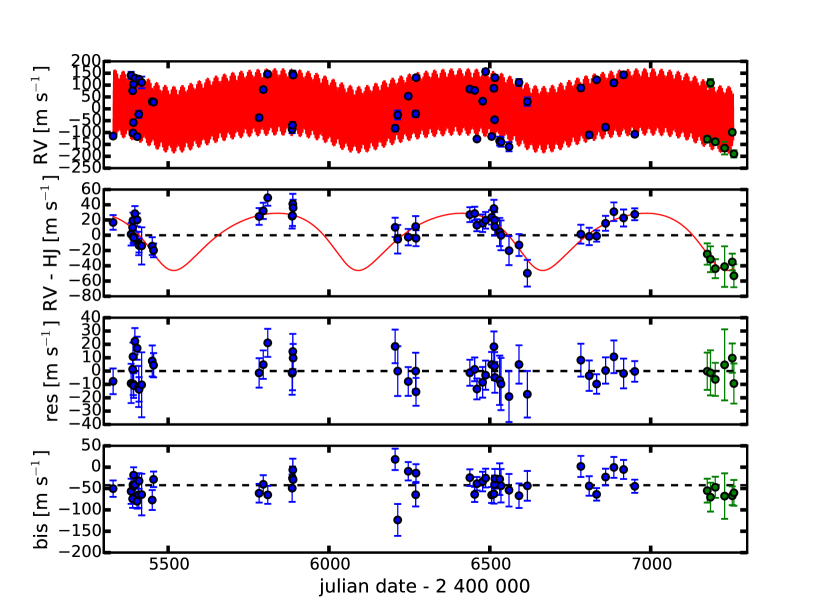
Figure 12: CORALIE data of WASP-47 plotted in time. Blue/Green dots: before/after the upgrade. Top panel: Radial velocities superimposed with the best fit model. Second panel: Residuals of the radial velocities after subtracting the hot Jupiter superimposed with the model for the second planet. Third panel: Residuals of the radial velocities after subtracting the two planets. Bottom panel: Bisector spans.

WASP-47 is a G9V star hosting a giant planet with a mass of 1.14 M_Jup and a period of 4.16 days (Hellier et al., 2012). The discovery paper includes 19 radial velocity measurements taken with CORALIE during two observing seasons. Ongoing monitoring revealed a possible third body, and after 46 observations over 4.44 years, the orbit of a second planet was clear. After subtracting the inner planet (hot Jupiter) from the radial velocity data, the analysis of the residuals using a Lomb-Scargle periodogram shows a clear peak around 550 days (see Fig. 1). The analysis of the residuals after subtracting the two-planet model shows no additional signal (see Fig. 12).

In November 2014, an upgrade of CORALIE was performed. The changes introduced an offset in the radial velocities. Since the orbit of the outer planet was not fully covered in phase, we collected six additional measurements from June to August 2015. One measurement was done right after the upgrade just before the star became unobservable but it suffered from daylight contamination and had to be discarded. For the analysis, the 2015 data are considered as an independent radial velocity data set.

2.2 Analysis

We combined the photometry data from EulerCAM (Gunn-$r^{\prime}$ filter) published in Hellier et al. (2012) with all the radial velocities from CORALIE and used an adaptive Markov chain Monte-Carlo (MCMC) fitting scheme to derive the system parameters of the two-planet model. We did not include the WASP photometry in our analysis because it has poor precision compared to EulerCAM and might suffer from spatial dilution from background stars. We used the most recent version of the code described in Gillon et al. (2012) and references therein. The jump parameters used in our analysis to characterise the transiting planet WASP-47b were

• the transit depth defined as the planet/star area ratio (d$F=(R_{\rm p}/R_{\star})^{2}$), where $R_{\rm p}$ and $R_{\star}$ are the planetary and stellar radius, respectively;

• the transit impact parameter in the case of a circular orbit ($b^{\prime}=a_{\rm b}\cos i_{\rm p,b}/R_{\star}$), where $a_{\rm b}$ and $i_{\rm p,b}$ are the semi-major axis and the inclination of the planetary orbit, respectively;

• the transit duration $T_{\rm 14}$, from first to last contact;

• the orbital period $P_{\rm b}$;

• the time of inferior conjunction $T_{\rm 0,b}$;

• the two parameters $\sqrt{e_{\rm b}}\,\cos\omega_{\rm b}$ and $\sqrt{e_{\rm b}}\,\sin\omega_{\rm b}$, where $e_{\rm b}$ is the eccentricity and $\omega_{\rm b}$ the argument of periastron;

• the parameter $K_{\rm 2,b}=K_{\rm b}\sqrt{1-e_{\rm b}^{2}}\,P_{\rm b}^{1/3}$, where $K_{\rm b}$ is the radial velocity semi-amplitude.

For the period $P_{\rm b}$ and time of inferior conjunction $T_{\rm 0,b}$, we imposed Gaussian priors defined by the values derived in Hellier et al. (2012), since we did not include the WASP photometry in our analysis. Uniform priors were assumed for the probability distribution functions of all the other jump parameters. The choices of jump parameters were optimised to reduce the dependencies between the parameters and thus to minimise the correlations. We checked that using $\sqrt{e}\,\cos\omega$ and $\sqrt{e}\,\sin\omega$ as jump parameters translates into a uniform prior on e and does not influence the results.

We modelled the limb-darkening with a quadratic law, where instead of the coefficients $u_{1}$ and $u_{2}$, we used the combinations $c_{1}=2\times u_{1}+u_{2}$ and $c_{2}=u_{1}-2\times u_{2}$ as jump parameters in order to minimise the correlation of the obtained uncertainties (Holman et al., 2006). We assumed normal priors on $u_{1}$ and $u_{2}$ with the values deduced from the tables by Claret & Bloemen (2011). As described in Gillon et al. (2012), we applied a correction factor $CF=1.32$ to the error bars of the photometric data to account for the red noise.

WASP-47 c does not have transit observations, the jump parameters used in our analysis to define the second orbit were

• the orbital period $P_{\rm c}$;

• the time of inferior conjunction $T_{\rm 0,c}$;

• the two parameters $\sqrt{e_{\rm c}}\cos\omega_{\rm c}$ and $\sqrt{e_{\rm c}}\sin\omega_{\rm c}$;

• the parameter $K_{\rm 2,c}=K_{\rm c}\sqrt{1-e_{\rm c}^{2}}\,P_{\rm c}^{1/3}$.

We assumed uniform priors on all those jump parameters.

The stellar density is derived at each step of the MCMC from Kepler’s third law and the values of the scale parameter $a_{\rm b}/R_{\star}$ and orbital period of WASP-47b (Winn et al., 2010). The stellar mass $M_{\star}$ is obtained thanks to a calibration (Enoch et al., 2010; Gillon et al., 2011) from well-constrained binary systems (Southworth, 2011). This empiric law is a function of $T_{\rm eff}$, $\rho_{\star}$ and [Fe/H]. We used Gaussian prior distributions for $T_{\rm eff}$ and [Fe/H], and the initial value for $\rho_{\star}$, based on the values derived by Mortier et al. (2013).

2.3 Results

The results presented in Table 1 have been obtained running five chains of 100 000 accepted steps. The derived values are the median and 1 $\sigma$ limits of the marginalised posterior distributions, considering a 20% burn-in phase. The acceptance fraction is $\sim$25% ($\sim$40% for the burn-in phase). We used the statistical test of Gelman & Rubin (1992) to check the convergence of the chains and get a potential scale reduction factor (PSRF) smaller than 1.01 for all the jump parameters. The autocorrelations are shorter than 2 000 steps except for the semi-amplitude and the eccentricity of the outer planet. The lack of data around the radial velocity minimum introduces a small degeneracy between these parameters. Their autocorrelations are $\sim$5 000 steps long. As we did not include additional transit light curves, we did not improve the determination of the transit parameters compared to Hellier et al. (2012). They are not given here for this reason. The best fit solution for the radial velocities is plotted in Fig. 2. The values provided in Table 1 are the median values of the posterior distributions and not the best fit values used in Fig. 2. To verify that the median values represent a self-consistent set of parameters, we compare the BIC (Bayesian Information Criterion) obtained using the median values and the best fit values. We obtain compatible results.

Including the data collected in 2015 allows to reduce the uncertainty on the eccentricity and semi-amplitude of the outer planet. All the other parameters remain unchanged compared to the results obtained with the first data set alone. The posterior distribution of the offset between the two data sets ($\Delta$RV = 18 $\pm$ 11 m s^-1) agrees with what has been observed on bright radial velocity standards.

The semi-amplitude of WASP-47 c is barely twice as large as the radial velocity uncertainties, and the phase coverage is incomplete. To validate the detection, we compared the results obtained when running the same MCMC with a model including only one planet. With the one-planet model, the reduced $\chi^{2}$ on the initial set of radial velocities is 2.7 and the residual r.m.s. 19.2 m s^-1. When fitting two planets, the corresponding reduced $\chi^{2}$ is 1.2 and the residual r.m.s. 10.6 m s^-1. The two-planet model is clearly preferable.

Figure 1: WASP-47 Lomb-Scargle periodogram of the residuals after subtracting Planet b. The dotted lines correspond to a false-alarm probability of 0.1%, 1%, and 10%.

Table 1: Median and 1-$\sigma$ limits of the posterior marginalised PDFs obtained for the WASP-47 system derived from our global MCMC analysis

MCMC Jump parameters
Star
$T_{\rm eff}$ [K]	5576 $\pm$ 68
[Fe/H]	0.36 $\pm$ 0.05
$c_{1}$	1.17 $\pm$ 0.03
$c_{2}$	$-0.02\pm$ 0.02
Planet b
$P_{\rm b}$ [d]	4.1591409 $\pm$ 0.0000072
$T_{\rm 0,b}$ – 2 450 000 [BJDTDB]	5764.3463 $\pm$ 0.0002
$\sqrt{e_{\rm b}}\,\cos\omega_{\rm b}$	0.04 $\pm$ 0.06
$\sqrt{e_{\rm b}}\,\sin\omega_{\rm b}$	0.01 $\pm$ 0.09
$K_{\rm 2,b}=K_{\rm b}\sqrt{1-e_{\rm b}^{2}}\,P_{\rm b}^{1/3}$ [m s-1 d1/3]	225.7 $\pm$ 3.6
Planet c
$P_{\rm c}$ [d]	572 $\pm$ 7
$T_{\rm 0,c}$ – 2 450 000 [BJDTDB]	5981 $\pm$ 16
$\sqrt{\rm e_{c}}\,\cos\omega_{\rm c}$	$-0.21$ $\pm$ 0.24
$\sqrt{\rm e_{c}}\,\sin\omega_{\rm c}$	0.16 $\pm$ 0.20
$K_{\rm 2,c}=K_{\rm c}\sqrt{1-e_{\rm c}^{2}}\,P_{\rm c}^{1/3}$ [m s-1 d1/3]	248 $\pm$ 43
Derived parameters
Star
$u_{1}$	0.462$\pm$0.014
$u_{2}$	0.242$\pm$0.010
Density $\rho_{\star}$ [$\rho_{\sun}$]	0.68 $\pm$ 0.06
Surface gravity $\log g_{\star}$ [cgs]	4.32 $\pm$ 0.05
Mass $M_{\star}$ [$M_{\sun}$]	1.026 $\pm$ 0.076
Radius $R_{\star}$ [$R_{\sun}$]	1.15 $\pm$ 0.04
Luminosity $L_{\star}$ [$L_{\sun}$]	1.14 $\pm$ 0.11
Planet b
Mass $M_{\rm p,b}$ [MJup]	1.13 $\pm$ 0.06
RV amplitude $K_{\rm b}$ [m s-1]	140 $\pm$ 2
Orbital eccentricity $e_{\rm b}$	¡ 0.026 (at 2 $\sigma$)
Orbital semi-major axis $a_{\rm b}$ [au]	0.051 $\pm$ 0.001
Density $\rho_{\rm p,b}$ [$\rho_{\rm J}$]	0.71 $\pm$ 0.08
Surface gravity $\log g_{\rm p,b}$ [cgs]	3.33 $\pm$ 0.03
Equilibrium temperature $T_{\rm eq,b}^{(*)}$ [K]	1275 $\pm$ 23
Planet c
Minimum mass $M_{\rm p,c}\sin i_{\rm p,c}$ [MJup]	1.24 $\pm$ 0.22
RV amplitude $K_{\rm c}$ [m s-1]	30 $\pm$ 6
Orbital eccentricity $e_{\rm c}$	0.13 $\pm$ 0.10
Argument of periastron $\omega_{\rm c}$ [°]	144 $\pm$ 53
Orbital semi-major axis $a_{\rm c}$ [au]	1.36 $\pm$ 0.04
Equilibrium temperature $T_{\rm eq,b}^{(*)}$ [K]	247 $\pm$ 5
$a_{\rm c}/R_{\star}$	255 $\pm$ 7

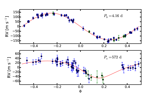
Figure 2: WASP-47 CORALIE radial velocity data (blue/green dots: before/after the upgrade) and best fit model (red line). Top: phase-folded on the period of the inner planet (outer planet subtracted). Bottom: phase-folded on the period of the outer planet (inner planet subtracted).

3 WASP-41 c

3.1 Observations

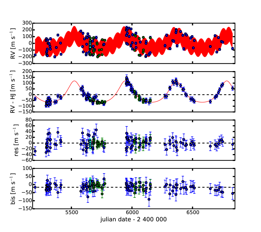
Figure 13: Radial velocity data of WASP-41 plotted in time. Blue: CORALIE; Green: HARPS; Cyan: RM sequence. Top panel: Radial velocities superimposed with the best fit model. Second panel: Residuals of the radial velocities after subtracting the hot Jupiter superimposed with the model for the second planet. Third panel: Residuals of the radial velocities after subtracting the two planets. Bottom panel: Bisector spans.

WASP-41 is a G8V star hosting a giant planet with a mass of 0.9 M_Jup and a period of 3.05 days (Maxted et al., 2011). The discovery paper includes 22 radial velocity measurements taken within four months (excluding the first point). The short time span of the observations did not allow for detecting any additional signal. We did a follow-up on the star and collected a total of 100 radial velocities with CORALIE over 4.46 years. The observations during the second season revealed an offset of $\sim$100 m s^-1 and triggered an intensive monitoring of the target. An additional planet on an eccentric orbit rapidly became apparent. Because of the significant eccentricity of the second planet combined with a period close to one year, we had to wait until the fifth year of follow-up to plan observations at the periastron with a good sampling. After subtracting the inner planet (hot Jupiter) from the radial velocity data, the analysis of the residuals using a Lomb-Scargle periodogram shows a clear peak around 400 days (see Fig. 3). The additional peaks present at $\sim$200 days and $\sim$130 days correspond to the two first harmonics $P/2$ and $P/3$. Such features are expected when applying frequency decomposition to eccentric signals, and WASP-41c has an eccentricity $e\sim 0.3$. The analysis of the residuals, after subtracting the two planets from the radial velocities, shows no additional periodic signal (see Fig. 13).

Figure 3: WASP-41 Lomb-Scargle periodogram of the residuals after subtracting Planet b. The dotted lines correspond to false-alarm probabilities of 0.1%, 1%, and 10%.

We used the HARPS spectrograph mounted on the 3.6-m telescope in La Silla to observe the Rossiter–McLaughlin effect induced by WASP-41 b during the transit on 3 Apr 2011. In addition to the Rossiter–McLaughlin observations, 30 measurements out of transit of WASP-41 were gathered with HARPS between Apr 2011 and Aug 2012 to confirm the second signal detected with CORALIE.

More transit light curves of WASP-41 b have been obtained since the publication of the discovery paper: with the Faulkes Telescope South (FTS) at Siding Spring Observatory and with the TRAPPIST telescope (Jehin et al., 2011) and the Danish telescope both in La Silla. Details of these observations can be found in Table 2.

Table 2: Additional transit observations of WASP-41b and applied correction factors.

Instrument	Filter	date	$CF$
FTS	PanSTARRS $z$	12 Apr 2011	1.8
TRAPPIST	$I+z$	21 Mar 2011	1.0
		02 Apr 2011	2.1
		12 May 2011	2.0
		09 Mar 2012	1.5
		19 Apr 2013	1.4
Danish	$R$	19 Apr 2013	2.2
		25 Apr 2013 (∗)	3.0

3.2 Study of stellar activity

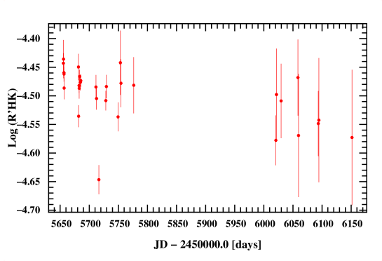
Figure 14: WASP-41 $\log R^{\prime}_{\rm HK}$ extracted from the HARPS spectra.

WASP-41 is known to be an active star (Maxted et al., 2011). In spite of the large amplitude of the second signal, we check that it is not due to a stellar magnetic cycle. For that purpose we searched for correlations between the radial velocities and spectral activity indicators. No variation is observed in the bisector span of the cross correlation function (Fig. 13 bottom panel). The full width at half maximum (FWHM) shows some variability, which is suspiciously similar to the radial velocities’ variability (periodicity close to 400 days). The $\log R^{\prime}_{\rm HK}$ extracted from the HARPS spectra, based on the photospheric Ca II (H & K) lines, indicates a mean value of $-4.483\pm 0.036$ characteristic of an active star. But no variation in the $\log R^{\prime}_{\rm HK}$ is visible during the two years of HARPS data (Fig. 14).

The emission in the H$\alpha$ line is a rather underused activity indicator to trace photospheric stellar activity. In their study, Cincunegui et al. (2007) concluded that the activity measured in the H$\alpha$ was not equivalent to the $R^{\prime}_{\rm HK}$ indicator. They did not measure similar correlations between the two indicators in their whole sample. Some of their stars showed correlations, when others showed no or anti-correlations. Using solar observations, Meunier & Delfosse (2009) demonstrated that the Ca II (H & K) and the H$\alpha$ emissions have different behaviours. During an active period when the filaments reach saturation, they observe a positive correlation between the indicators. On the other hand, during moderate active periods, the filaments counteract the effect of plages on the H$\alpha$ measurements, leading to weak or negative correlations. Gomes da Silva et al. (2014) conclude that active stars with a mean $\log R^{\prime}_{\rm HK}\geq-4.7$ systematically show a positive correlation between the Ca II (H & K) and H$\alpha$ flux.

Since WASP-41 is a very active star with $\log R^{\prime}_{\rm HK}\geq-4.7$, it is reasonable to use H$\alpha$ as an activity indicator. The motivation to use this band is that it is located in the red part of the stellar spectrum where a high signal-to-noise ratio can be obtained from the CORALIE spectra. As suggested in Cincunegui et al. (2007), we measured the H$\alpha$ emission at 6562.808 $\mathrm{\SIUnitSymbolAngstrom}$ and the continuum centred at 6605 $\mathrm{\SIUnitSymbolAngstrom}$ and averaged on a window 20 $\mathrm{\SIUnitSymbolAngstrom}$ wide. Unlike Cincunegui et al. (2007) we extracted the H$\alpha$ from a 0.6 $\mathrm{\SIUnitSymbolAngstrom}$ wide band instead of 1.5 $\mathrm{\SIUnitSymbolAngstrom}$.

The H$\alpha$ index reveals a time variation similar to the one observed on the FWHM (Fig. 4) that can be modelled by a third-order trend in time. It is then reasonable to conclude that we are observing the magnetic cycle of WASP-41. After subtracting the third-order trend, we analysed the Lomb-Scargle periodogram of the residuals in the FWHM. A clear peak appears at exactly one year (see Fig. 5). The same one-year signal in the FWHM has been observed on the brighter stars also regularly observed with CORALIE, as well as with similar instruments (SOPHIE, HARPS). When we look at the Lomb-Scargle periodogram of the H$\alpha$ index after subtracting the long-term trend, a peak appears at $\sim$18 days (see Fig. 6). Interestingly, this corresponds to the rotation period of the star derived from the WASP photometry by Maxted et al. (2011).

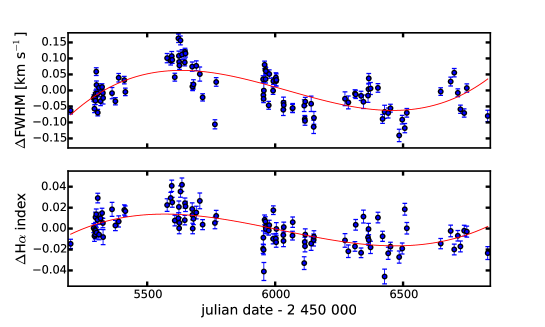
Figure 4: Magnetic cycle of WASP-41. Top: FWHM of the CCF from the CORALIE measurements. Bottom: H$\alpha$ index extracted from the CORALIE spectra. The red lines correspond to the fitted third-order trend.

Figure 5: WASP-41 Lomb-Scargle periodogram of the FWHM after subtracting the third-order trend. A clear peak is present at 1 year. The dotted lines correspond to a false-alarm probability of 0.1%, 1%, and 10%.

Figure 6: WASP-41 Lomb-Scargle periodogram of the H$\alpha$ index after subtracting the third-order trend. A peak is present at $\sim$18 days, corresponding to the photometric rotation period. The dotted lines correspond to a false-alarm probability of 0.1%, 1%, and 10%.

Encouraged by the interesting result obtained using the H$\alpha$ index on WASP-41, we looked at the similarly active star CoRoT-7 (with $\log R^{\prime}_{\rm HK}=-4.62\geq-4.7$). Queloz et al. (2009) note that CoRoT-7 shows strong variability in the FWHM, comparable to what is observed on WASP-41. CoRoT-7 benefitted from simultaneous photometric and spectroscopic observations (see Haywood et al., 2014). We extracted the H$\alpha$ index from the HARPS spectra of CoRoT-7 in the same way as WASP-41. A very clear correlation is observed between the H$\alpha$ index and the FWHM (see Fig. 7). After subtracting a third-order trend, very likely due to the magnetic cycle, a signal appears at $\sim$23 days, corresponding to the photometric rotation period of the star. This similar result confirms that the H$\alpha$ index is a good activity indicator for such active stars.

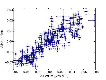
Figure 7: Correlation between the H$\alpha$ index and the FWHM from HARPS data of CoRoT-7.

The 400-day signal detected in the radial velocities is detected neither in the FWHM nor in the H$\alpha$. Its origin is most likely due to the presence of a second planetary companion.

3.3 Analysis

As we did with WASP-47, we simultaneously fitted the transit light curves and the radial velocity measurements with an MCMC algorithm. To define the priors for the limb-darkening coefficients of the non-standard TRAPPIST $I+z$ filter, we took the average of the values of the standard filters $Ic$ and $z^{\prime}$, and the quadratic sums of their errors. We did not include the FTS photometry from the discovery paper in our analysis because it suffered from poor weather conditions. As suggested by Gillon et al. (2012), we included a quadratic polynomial in time to model the transit light curves (except the fourth TRAPPIST and the first Danish transit observations).

The observations with TRAPPIST on 21 Mar 2011 and 9 Mar 2012 suffered from malfunctions of the autofocus. As a consequence, the FWHM of the images varied a lot. To correct for this effect, we added a third-order and a quadratic polynomial in FWHM, respectively, to model those two light curves. The TRAPPIST observation on 19 Apr 2013 experienced a meridian flip that we modelled including an offset for that light curve. The TRAPPIST light curve from the 2 Apr 2011 and the Danish one from the 25 Apr 2013 obviously exhibited stellar spot crossings. We visually identified the affected parts of the light curves and decreased their weights by increasing the corresponding errors. In general, we applied a correction factor to the error bars of the light curves to account for red noise (values listed in Table. 2).

To improve the fit of the radial velocities and decrease the effects of stellar activity, we included a quadratic polynomial in the FWHM of the radial velocities from CORALIE. Then we quadratically added a ”jitter” noise of 13.2 m s^-1 to the error bars to equal the mean error with the standard deviation of the best-fit model residuals. For the HARPS data (not including the RM sequence), we added a linear dependency in FWHM and a quadratic polynomial in bisector. We also added a ”jitter” noise of 6.7 m s^-1 to the radial velocity error bars. The baselines in FWHM and bisector were determined by comparing the BIC and the residual jitter obtained when running short chains with various models.

We modelled the Rossiter–McLaughlin effect following the equations of Giménez (2006). We used $\sqrt{v\,\sin I_{\star}}\,\cos\beta$, and $\sqrt{v\,\sin I_{\star}}\,\sin\beta$ as jump parameters, where $\beta$ is the projected angle between the stellar spin axis and the planet’s orbital axis, and $v\,\sin I_{\star}$ is the projected rotational velocity. The Rossiter–McLaughlin sequence is fitted as an independent dataset to mitigate the effect of stellar activity. We did not need to add any ”jitter” or dependency on other parameters to these data. Owing to the low transit impact parameter $b_{\rm tr}$, there was a strong degeneracy between $\beta$ and $v\,\sin I_{\star}$ (see Triaud et al., 2011; Anderson et al., 2011). We imposed a normal prior on $v\,\sin\,I_{\star}$ to avoid unphysical solutions. Indeed from an MCMC with no prior on the $v\,\sin I_{\star}$ we obtain $\beta=-48\degr\pm 29\degr$, and $v\,\sin\,I_{\star}=3.5^{+10.0}_{-1.0}$ km s^-1 with $v\,\sin\,I_{\star}$ getting higher than 100 km s^-1, clearly inconsistent with the spectral analysis. The value derived for $\beta$ is strongly dependent on the value of the prior for $v\,\sin\,I_{\star}$

The priors used for $T_{\rm eff}$ and [Fe/H] are defined with the values from Mortier et al. (2013). For the $v\,\sin I_{\star}$ we revised the value derived by Doyle et al. (2014), using the stellar parameters from Mortier et al. (2013) to estimate the macroturbulence. Therefore we used $v\,\sin I_{\star}=2.66\pm 0.28$ km s^-1 as a normal prior. Since we benefitted from transit observations that span more than three years, we did not use a prior on the period and time of inferior conjunction $T_{\rm 0,b}$ of the transiting planet.

3.4 Results

We present in Table 3 the median and 1 $\sigma$ limits of the marginalised posterior distributions after running five chains of 100 000 accepted steps (considering a 20% burn-in phase). The acceptance rate is $\sim$25% ($\sim$40% for the burn-in phase). The convergence of the chains is validated by the test of Gelman & Rubin (1992) (PSFR better than 1.01), and the autocorrelations are shorter than 2 000 steps. Including the second planet in the model undoubtedly improves the fit. The r.m.s. of the CORALIE data after the two-planet fit is ten times smaller than after a one-planet fit. The best fit solution is plotted in Fig. 8 for the transit light curves and in Fig. 9 for the radial velocities. Again, the values provided in Table 3 are not the ones used in Figs. 9 and 8. We checked that they represent a self-consistent set of parameters by comparing the BIC using both sets of values (best fit and median of the posterior distribution) and get compatible results.

Table 3: Median and 1 $\sigma$ limits of the posterior marginalised PDFs obtained for the WASP-41 system derived from our global MCMC analysis

MCMC Jump parameters
Star
$T_{\rm eff}$ [K]	5545 $\pm$ 33
[Fe/H]	0.06 $\pm$ 0.02
$c_{1,z^{\prime}}$	0.819 $\pm$ 0.009
$c_{2,z^{\prime}}$	$-0.230\pm$ 0.006
$c_{1,I+z}$	0.85 $\pm$ 0.04
$c_{2,I+z}$	$-0.19\pm$ 0.04
$c_{1,R}$	1.08 $\pm$ 0.01
$c_{2,R}$	$-0.09\pm$ 0.01
Planet b
Planet/star area ratio $(R_{\rm p}/R_{\star})^{2}$ [%]	1.87 $\pm$ 0.01
$b^{\prime}=a_{\rm b}\cos i_{\rm p,b}/R_{\star}$	0.10 $\pm$ 0.06
$T_{\rm 14}$[d]	0.1099$\pm$0.0002
$P_{\rm b}$ [d]	3.0524040 $\pm$ 0.0000009
$T_{\rm 0,b}$ – 2 450 000 [BJDTDB]	6014.9936 $\pm$ 0.0001
$\sqrt{e_{\rm b}}\,\cos\omega_{\rm b}$	$0.002\pm$ 0.048
$\sqrt{e_{\rm b}}\,\sin\omega_{\rm b}$	0.059 $\pm$ 0.074
$K_{\rm 2,b}=K_{\rm b}\sqrt{1-e_{\rm b}^{2}}\,P_{\rm b}^{1/3}$ [m s-1 d1/3]	199.7 $\pm$ 2.3
$\sqrt{v\,\sin I_{\star}}\,\cos\beta$	1.42 $\pm$ 0.10
$\sqrt{v\,\sin I_{\star}}\,\sin\beta$	$-0.78^{+0.38}_{-0.28}$
Planet c
$P_{\rm c}$ [d]	421 $\pm$ 2
$T_{\rm 0,c}$ – 2 450 000 [BJDTDB]	6011 $\pm$ 3
$\sqrt{\rm e_{c}}\,\cos\omega_{\rm c}$	0.53 $\pm$ 0.02
$\sqrt{\rm e_{c}}\,\sin\omega_{\rm c}$	$-0.07\pm$ 0.06
$K_{\rm 2,c}=K_{\rm c}\sqrt{1-e_{\rm c}^{2}}\,P_{\rm c}^{1/3}$ [m s-1 d1/3]	676 $\pm$ 21
Derived parameters
Star
$u_{1,z^{\prime}}$	0.282 $\pm$ 0.005
$u_{2,z^{\prime}}$	0.256 $\pm$ 0.002
$u_{1,I+z}$	0.30 $\pm$ 0.02
$u_{2,I+z}$	0.25 $\pm$ 0.02
$u_{1,R}$	0.416 $\pm$ 0.006
$u_{2,R}$	0.252 $\pm$ 0.004
Density $\rho_{\star}$ [$\rho_{\sun}$]	1.41 $\pm$ 0.05
Surface gravity $\log g_{\star}$ [cgs]	4.53 $\pm$ 0.02
Mass $M_{\star}$ [$M_{\sun}$]	0.93 $\pm$ 0.07
Radius $R_{\star}$ [$R_{\sun}$]	0.87 $\pm$ 0.03
Luminosity $L_{\star}$ [$L_{\sun}$]	0.64 $\pm$ 0.04
Projected rotation velocity $v\,\sin\,I_{\star}$ [km s-1]	2.64 $\pm$ 0.25
Planet b
Mass $M_{\rm p,b}$ [MJup]	0.94$\pm$0.05
Radius $R_{\rm p,b}$ [RJup]	1.18 $\pm$ 0.03
RV amplitude $K_{\rm b}$ [m s-1]	138$\pm$2
Orbital eccentricity $e_{\rm b}$	¡ 0.026 (at 2 $\sigma$)
Orbital semi-major axis $a_{\rm b}$ [au]	0.040 $\pm$ 0.001
Orbital inclination $i_{\rm p,b}$ [°]	89.4 $\pm$ 0.3
Transit impact parameter $b_{\rm tr}$	0.10 $\pm$ 0.06
Projected orbital obliquity $\beta$ [°]	$-29^{+14}_{-10}$
Density $\rho_{\rm p,b}$ [$\rho_{\rm J}$]	0.56 $\pm$ 0.03
Surface gravity $\log g_{\rm p,b}$ [cgs]	3.24 $\pm$ 0.01
Equilibrium temperature $T_{\rm eq,b}^{(*)}$ [K]	1244 $\pm$ 10
Planet c
Minimum mass $M_{\rm p,c}\sin i_{\rm p,c}$ [MJup]	3.18 $\pm$ 0.20
RV amplitude $K_{\rm c}$ [m s-1]	94 $\pm$ 3
Orbital eccentricity $e_{\rm c}$	0.294 $\pm$ 0.024
Argument of periastron $\omega_{\rm c}$ [°]	353 $\pm$ 6
Orbital semi-major axis $a_{\rm c}$ [au]	1.07 $\pm$ 0.03
Equilibrium temperature $T_{\rm eq,b}^{(*)}$ [K]	241 $\pm$ 2
$a_{\rm c}/R_{\star}$	265 $\pm$ 3

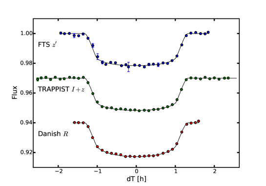
Figure 8: WASP-41b transit data (blue: FTS $z^{\prime}$; green: TRAPPIST $I+z$; red: Danish $R$) and best fit model (black line). The TRAPPIST light curve was obtained by binning the data from five transit observations, and the Danish one from one full and one partial transit observations. Each point corresponds to a 7.2 min bin.

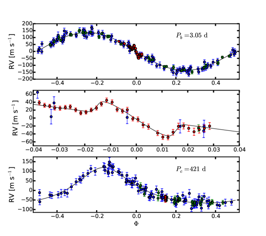
Figure 9: WASP-41 radial velocity data (blue: CORALIE, green: HARPS; red: HARPS RM sequence) and best fit model (black line). Top: Phase-folded on the period of the inner planet (outer planet subtracted). Middle: Zoom on the Rossiter–McLaughlin effect. Bottom: Phase-folded on the period of the outer planet (inner planet subtracted).

The best-fitting model suggests a misaligned planet with a projected orbital obliquity of $\beta=-28\degr\pm 13\degr$. However, the uncertainties are large (see Fig. 10), and the data do not allow an aligned orbit to be excluded ($P(|\beta|<20\degr)\sim 24\%$). The rotation velocity expected from the photometric rotation period of the star ($\sim$ 2.44 km s^-1) is compatible within the error bars with the spectroscopic $v\,\sin I_{\star}$ (2.64 $\pm$ 0.25 km s^-1), suggesting that the star is equator-on. That reinforces the possibility of an aligned planet.

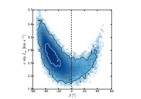
Figure 10: Posterior distribution of $\beta$ and $v\,\sin I_{\star}$ for WASP-41 b on logarithmic scale. We impose a prior of $2.66\pm 0.28$ km s^-1 on $v\,\sin I_{\star}$. The contours correspond to the 1-, 2-, and 3-$\sigma$ confidence limits for each parameter, and include 39.3%, 86.5%, and 98.9% of the MCMC steps, respectively.

4 Discussion

We have shown that finding long-period planets with instruments such as CORALIE is still possible around active stars. Recognising the periodic structure of activity-related signals is essential to avoiding false detections. While spots or plages induce signals at the rotation period of the star, the evolution of their coverage of the stellar surface is correlated with the magnetic cycle of the star. Such cycles have periods of several years and must be distinguished from long-period companions. Lovis et al. (2011) studied the effect of magnetic cycles on the radial velocity measurements from the HARPS planet search sample. They derived empirical models of correlations between $R^{\prime}_{\rm HK}$ and radial velocities, FWHM, contrast, and bisector spans, depending on the effective temperature $T_{\rm eff}$ and metallicity [Fe/H] of the star. However, their sample only contains ’quiet’ stars because they are the preferred targets for planet searches. They consider only a handful of targets with a mean $\log R^{\prime}_{\rm HK}>-4.7$, so their results cannot be applied to active stars. The CORALIE search for planets observes stars with a broader range of $\log R^{\prime}_{\rm HK}$ than the HARPS one. While the emission in the Ca II (H & K) lines is hard to extract from the CORALIE spectra, we have shown that the emission in the H$\alpha$, which is easy to measure, is a good indicator of activity for stars with $\log R^{\prime}_{\rm HK}>-4.7$. A systematic study of the correlation between the H$\alpha$ emission and the radial velocities of active stars could help to estimate the influence of magnetic cycles on radial velocity measurements of active stars.

The transit technique has led to the discovery of more than 200 hot Jupiters, while only $\sim$30 have been discovered by Doppler surveys. A total of nine multiple planetary systems that include a hot Jupiter (with a ¡ 0.1 au) and a second planet with a fully probed orbit, are known (source: exoplanet.eu). Among them, four were discovered by radial velocity surveys and five by transit surveys. Those multiple systems represent $\sim$13% of the known hot Jupiters found by radial velocities and only $\sim$2% of those found by transit searches. The most obvious explanation for this difference is historical. Radial velocity surveys started discovering hot Jupiters well before transit surveys. The hot Jupiters discovered by radial velocities have been followed for more than ten years, allowing the detection of very wide companions (P ¿ 9 years). The dedicated large transit surveys (mainly HATNet and SuperWASP) started to efficiently discover hot Jupiters about six years ago, allowing only the characterisation of relatively close companions. If we exclusively consider companions within 2 au, the rate of hot Jupiters with companions from the Doppler sample is divided by two.

The difference in the rates of detected additional planets in systems with a hot Jupiter may also be explained by the different observing strategies used in Doppler and transit surveys. The discovery of a hot Jupiter based on radial velocity data requires a large number of observations because the observer has no prior information on the planet. About typically ten radial velocity observations are carried out to confirm the existence of a hot Jupiter previously detected by transit. In that case the observer knows the period of the planet and can plan the radial velocity observations in order to measure the radial velocity orbit very efficiently. This means that, on average, hot Jupiters discovered by the Doppler technique benefit from a larger number of radial velocity measurements than those discovered by transits. Increasing the number of radial velocity measurements makes the detection of longer period planetary companions easier.

In the beginning of the WASP follow-up with CORALIE, we started a systematic search for long-period companions around the WASP targets with a confirmed hot Jupiter. We have followed more than 100 WASP host stars for durations of two to eight years, including about 90 targets followed for more than three years. The publication of this work is in preparation (Neveu-VanMalle et al. in prep). In this sample only two stars with a hot Jupiter have been found to host a second planet that has completed at least one orbit. We still have a lack of multiple systems within 2 au compared to the hot Jupiters discovered by radial velocity surveys.

Detectability thresholds can contribute to explain the observed discrepancy. Figure 11 shows the multiple planetary systems (with fully characterised orbits) that include a hot Jupiter, distributed in a plot of semi-major axis versus mass. The symbols located on the left-hand side of the plot (a ¡ 0.1 au) are the hot Jupiters, and the symbols on the right-hand side (a ¿ 0.1 AU) are the long-period planets. The dotted lines were drawn to visualise which planets are part of the same system. We notice that except for WASP-47 c, only the long-period planets from the Doppler-survey systems have semi-amplitudes smaller than 80 m s^-1. Indeed, Doppler surveys target small samples of bright stars, while transit surveys target large samples of fainter stars. Besides being brighter, radial velocity targets are in general less active than transit targets. This means that a better precision can be obtained on the radial velocity measurements of stars from Doppler surveys. With a higher signal-to-noise ratio, detecting smaller signals is easier around brighter quiet stars. Smaller long-period planets might exist around stars with a known transiting hot Jupiter, but they are out of reach of current surveys.

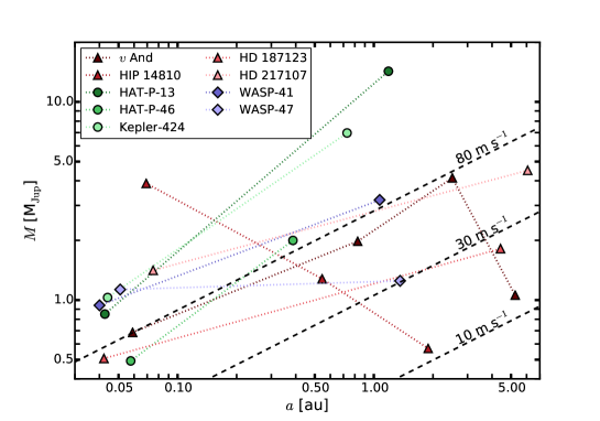
Figure 11: Known multiple planetary systems with fully probed orbits including a hot Jupiter (a ¡ 0.1 au). Triangles: hot Jupiter found by radial velocity surveys. Circles: Hot Jupiters found by transit surveys. Diamonds: systems presented in this paper. The black dashed lines correspond to a radial velocity semi-amplitude of 10 m s^-1, 30 m s^-1, and 80 m s^-1 assuming a circular orbit around a 1-M_☉ star. Most of these planets were detected only by radial velocities, thus we are plotting the minimum mass $M\sin i$ instead of the true mass $M$.

Knowing that WASP-47b and WASP-41b are transiting, it is natural to wonder if their outer planetary companions transit as well. If we assume that the inclination of the outer planet is uniformly distributed, independently of the inclination of the hot Jupiter, the transit probability is $\sim$0.4% for WASP-47c and $\sim$0.6% for WASP-41c (using Kane & von Braun, 2008). If we assume a coplanar system where the orbit of the outer planet can be uniformly distributed around $5\degr$ from the orbit of the hot Jupiter, we obtain a transit probability of $\sim$6% in both cases. Detecting the transit of the outer planet would bring strong evidence that the hot Jupiter had migrated inside the disk via gap opening (Lin et al., 1996; Marzari & Nelson, 2009). However, a non-detection would not be sufficient to infer a high mutual inclination between the orbits of the planets, which would be evidence of a migration scenario involving dynamical interactions (Rasio & Ford, 1996; Fabrycky & Tremaine, 2007; Nagasawa et al., 2008; Matsumura et al., 2010; Naoz et al., 2011).

The next predicted inferior conjunctions for WASP-47c are 2 Nov 2016 $\pm$ 30 d and 24 May 2018 $\pm$ 43 d, with an expected transit duration of $\sim$18 h. A radial velocity follow-up is ongoing in order to improve the ephemeris. The next predicted inferior conjunction for WASP-41c (02 Nov 2016 $\pm$ 7 d) cannot be observed by ground-based facilities because the star is close to the Sun. The two following ones are 12 Jan 2018 $\pm$ 8 d and 3 Mar 2019 $\pm$ 10 d with an expected transit duration of $\sim$13 h.

Recently, (Becker et al., 2015) have announced the detection of two additional transiting planets around WASP-47. We checked if the nine-day planet could be detected in our set of radial velocities. Unfortunately, the expected amplitude of the signal is below the sensitivity of CORALIE for such faint stars. The geometry of this system favours disc migration theories because scattering is unlikely to have kept the inner system coplanar. Sanchis-Ojeda et al. (2015) have recently announced a low stellar obliquity for WASP-47 that reinforces the disc-migration hypothesis. Recent results have shown that Kozai interactions do not affect multi-planetary systems. In this case the outer planet could have ‘protected’ the inner planets from secular interactions. This system brings fundamental constraints for planetary formation and migration theories.

Appendix A Additional plots

Appendix B MCMC initial values and priors

Table 4: Initial values and priors for WASP-47

Parameter	Value	Prior
$M_{\star}$ [$M_{\sun}$]	1.07 $\pm$ 0.10 1	$\geq 0$
$T_{\rm eff}$ [K]	5576 $\pm$ 68 1	Gaussian
[Fe/H]	0.36 $\pm$ 0.05 1	Gaussian
$u_{1}$	0.4584 $\pm$ 0.0144 2	Gaussian, $u_{1}+u_{2}<1$ 4
$u_{2}$	0.2417 $\pm$ 0.0086 2	Gaussian, $u_{1,}+u_{2}<1$ 4
$P_{\rm b}$ [d]	4.1591399 $\pm$0.0000072 3	Gaussian
$T_{\rm 0,b}$ – 2 450 000 [BJDTDB]	5764.34602 $\pm$ 0.00022 3	Gaussian
$(R_{\rm p}/R_{\star})^{2}$ [%]	1.051 $\pm$ 0.014 3	uniform $\geq 0$
$T_{\rm 14}$[d]	0.14933 $\pm$ 0.00065 3	uniform $\geq 0$
$b_{\rm tr}$	0.14 $\pm$ 0.11 3	uniform on $b^{\prime}=a_{\rm b}\cos i_{\rm p,b}/R_{\star}$, $0\leq b_{\rm tr}\leq a_{\rm b}/R_{\star}$
$K_{\rm b}$ [m s-1]	136.0 $\pm$ 5 3	uniform on $K_{\rm 2,b}=K_{\rm b}\sqrt{1-e_{\rm b}^{2}}\,P_{\rm b}^{1/3}$ and $\geq 0$
$e_{\rm b}$	0	uniform on $\sqrt{e_{\rm b}}\,\cos\omega_{\rm b}$ and $\sqrt{e_{\rm b}}\,\sin\omega_{\rm b}$, if ¿ 1 then $e_{\rm b}$ = 0.999
$\omega_{\rm b}$	0	uniform on $\sqrt{e_{\rm b}}\,\cos\omega_{\rm b}$ and $\sqrt{e_{\rm b}}\,\sin\omega_{\rm b}$
$P_{\rm c}$ [d]	571 $\pm$ 8	uniform 0 d $\leq P\leq$ 1000 yr
$T_{\rm 0,c}$ – 2 450 000 [BJDTDB]	5983 $\pm$ 26	uniform
$K_{\rm c}$ [m s-1]	34 $\pm$ 10	uniform on $K_{\rm 2,c}=K_{\rm c}\sqrt{1-e_{\rm c}^{2}}\,P_{\rm c}^{1/3}$ and $\geq 0$
$e_{\rm c}$	0.2 $\pm$ 0.2	uniform on $\sqrt{e_{\rm c}}\,\cos\omega_{\rm c}$ and $\sqrt{e_{\rm c}}\,\sin\omega_{\rm c}$, if ¿ 1 then $e_{\rm c}$ = 0.999
$\omega_{\rm c}$	0	uniform on $\sqrt{e_{\rm c}}\,\cos\omega_{\rm c}$ and $\sqrt{e_{\rm c}}\,\sin\omega_{\rm c}$

¹ From Mortier et al. (2013). ² Interpolated from Claret & Bloemen (2011). ³ From Hellier et al. (2012). ⁵ See Kipping (2013).

Table 5: Initial values and priors for WASP-41

Parameter	Value	Prior
$M_{\star}$ [$M_{\sun}$]	0.90 $\pm$ 0.07 1	$\geq 0$
$T_{\rm eff}$ [K]	5546 $\pm$ 33 1	Gaussian
[Fe/H]	0.06 $\pm$ 0.02 1	Gaussian
$u_{1,z^{\prime}}$	0.2817 $\pm$ 0.0044 2	Gaussian, $u_{1,z^{\prime}}+u_{2,z^{\prime}}<1$ 5
$u_{2,z^{\prime}}$	0.2559 $\pm$ 0.0022 2	Gaussian, $u_{1,z^{\prime}}+u_{2,z^{\prime}}<1$ 5
$u_{1,I+z}$	0.3090 $\pm$ 0.0340 2	Gaussian, $u_{1,I+z}+u_{2,I+z}<1$ 5
$u_{2,I+z}$	0.2510 $\pm$ 0.0170 2	Gaussian, $u_{1,I+z}+u_{2,I+z}<1$ 5
$u_{1,R}$	0.4144 $\pm$ 0.0065 2	Gaussian, $u_{1,R}+u_{2,R}<1$ 5
$u_{2,R}$	0.2520 $\pm$ 0.0037 2	Gaussian, $u_{1,R}+u_{2,R}<1$ 5
$v\,\sin\,I_{\star}$ [km s-1]	2.66 $\pm$ 0.28 3	Gaussian
$P_{\rm b}$ [d]	3.052401 $\pm$ 0.000004 4	uniform 0 d $\leq P\leq$ 1000 yr
$T_{\rm 0,b}$ – 2 450 000 [BJDTDB]	6014.991 $\pm$ 0.001 4	uniform
$(R_{\rm p}/R_{\star})^{2}$ [%]	1.86 $\pm$ 0.04 4	uniform $\geq 0$
$T_{\rm 14}$[d]	0.108 $\pm$ 0.002 4	uniform $\geq 0$
$b_{\rm tr}$	0.40 $\pm$ 0.15 4	uniform on $b^{\prime}=a_{\rm b}\cos i_{\rm p,b}/R_{\star}$, $0\leq b_{\rm tr}\leq a_{\rm b}/R_{\star}$
$K_{\rm b}$ [m s-1]	135.0 $\pm$ 8 4	uniform on $K_{\rm 2,b}=K_{\rm b}\sqrt{1-e_{\rm b}^{2}}\,P_{\rm b}^{1/3}$ and $\geq 0$
$e_{\rm b}$	0	uniform on $\sqrt{e_{\rm b}}\,\cos\omega_{\rm b}$ and $\sqrt{e_{\rm b}}\,\sin\omega_{\rm b}$, if ¿ 1 then $e_{\rm b}$ = 0.999
$\omega_{\rm b}$	0	uniform on $\sqrt{e_{\rm b}}\,\cos\omega_{\rm b}$ and $\sqrt{e_{\rm b}}\,\sin\omega_{\rm b}$
$\beta$ [°]	0	uniform on $\sqrt{v\,\sin I_{\star}}\,\cos\beta$ and $\sqrt{v\,\sin I_{\star}}\,\sin\beta$
$P_{\rm c}$ [d]	418 $\pm$ 3	uniform 0 d $\leq P\leq$ 1000 yr
$T_{\rm 0,c}$ – 2 450 000 [BJDTDB]	6006 $\pm$ 10	uniform
$K_{\rm c}$ [m s-1]	94 $\pm$ 4	uniform on $K_{\rm 2,c}=K_{\rm c}\sqrt{1-e_{\rm c}^{2}}\,P_{\rm c}^{1/3}$ and $\geq 0$
$e_{\rm c}$	0.3 $\pm$ 0.05	uniform on $\sqrt{e_{\rm c}}\,\cos\omega_{\rm c}$ and $\sqrt{e_{\rm c}}\,\sin\omega_{\rm c}$, if ¿ 1 then $e_{\rm c}$ = 0.999
$\omega_{\rm c}$	0	uniform on $\sqrt{e_{\rm c}}\,\cos\omega_{\rm c}$ and $\sqrt{e_{\rm c}}\,\sin\omega_{\rm c}$

¹ From Mortier et al. (2013). ² Interpolated from Claret & Bloemen (2011). ³ Updated from Doyle et al. (2014). ⁴ From Maxted et al. (2011). ⁵ See Kipping (2013).

Appendix C Radial velocity data

Table 6: New radial velocities for WASP-47

BJD – 2 450 000	RV	$\sigma_{\rm RV}$	FWHM	Bis
(d)	(km s-1)	(km s-1)	(km s-1)	(km s-1)
6205.690749	$-27.16568$	0.01258	8.54665	$0.01824$
6213.632998	$-27.10977$	0.01866	8.50854	$-0.12360$
6246.539542	$-27.03050$	0.01077	8.52734	$-0.00957$
6269.531829	$-27.10498$	0.01370	8.60976	$-0.06453$
6270.530518	$-26.95272$	0.01043	8.56773	$-0.01388$
6437.858225	$-27.00067$	0.00972	8.52917	$-0.02456$
6452.924978	$-27.00623$	0.00890	8.56443	$-0.06375$
6459.924071	$-27.21081$	0.00784	8.56435	$-0.03869$
6477.721354	$-27.05162$	0.01149	8.59406	$-0.03366$
6486.844362	$-26.92702$	0.01094	8.52159	$-0.02556$
6505.757749	$-27.20042$	0.00939	8.55957	$-0.06514$
6512.745209	$-26.99712$	0.01142	8.49187	$-0.06260$
6514.752564	$-27.12983$	0.01053	8.50852	$-0.04074$
6515.749341	$-26.95270$	0.01151	8.53025	$-0.02725$
6530.629824	$-27.21972$	0.01850	8.54674	$-0.02802$
6534.789870	$-27.22405$	0.01955	8.57303	$-0.04356$
6559.713758	$-27.24359$	0.01907	8.51742	$-0.05402$
6590.650676	$-26.97269$	0.01437	8.51798	$-0.06681$
6616.574051	$-27.05365$	0.01745	8.54661	$-0.04370$
6782.899610	$-26.99561$	0.01233	8.53542	$0.00179$
6808.876282	$-27.19380$	0.01140	8.54211	$-0.04406$
6831.876641	$-26.96141$	0.00732	8.57188	$-0.06365$
6859.804354	$-27.16125$	0.00982	8.48966	$-0.02312$
6885.631966	$-26.97427$	0.01222	8.57285	$-0.00047$
6915.753320	$-26.94052$	0.01116	8.51941	$-0.00544$
6950.553823	$-27.19106$	0.00775	8.48781	$-0.04470$
CORALIE upgrade
7175.831586	$-27.17962$	0.01397	8.47192	$-0.05504$
7185.803516	$-26.94267$	0.01691	8.53709	$-0.07024$
7200.842220	$-27.19041$	0.01242	8.48536	$-0.04705$
7229.724940	$-27.21735$	0.02664	8.49685	$-0.06773$
7253.631858	$-27.15060$	0.01096	8.50363	$-0.06696$
7258.670969	$-27.24158$	0.01503	8.50061	$-0.06009$

Table 7: New radial velocities for WASP-41

BJD – 2 450 000	RV	$\sigma_{\rm RV}$	FWHM	Bis	$\log R^{\prime}_{\rm HK}$	$\sigma_{\log R^{\prime}_{\rm HK}}$
(d)	(km s-1)	(km s-1)	(km s-1)	(km s-1)
CORALIE
5577.833651	3.53952	0.01033	8.81258	$-0.04113$
5591.760168	3.30884	0.00989	8.80484	$-0.01806$
5595.802071	3.50882	0.01022	8.81885	$0.00150$
5597.776083	3.22930	0.00773	8.80704	$-0.02692$
5607.721786	3.41489	0.00873	8.75296	$-0.01255$
5621.850786	3.20236	0.00929	8.87451	$-0.00206$
5623.709905	3.45711	0.01054	8.81959	$0.00608$
5624.829879	3.20966	0.00976	8.80052	$-0.00711$
5625.826430	3.34101	0.00878	8.78968	$-0.03361$
5629.892800	3.45361	0.00973	8.86781	$-0.01814$
5635.815355	3.50088	0.01104	8.82368	$-0.07613$
5646.754274	3.22713	0.00777	8.79920	$-0.01367$
5647.630652	3.46375	0.00793	8.83207	$-0.00998$
5649.657082	3.19961	0.00800	8.82716	$-0.01678$
5675.784327	3.38673	0.01022	8.78597	$0.01963$
5676.605991	3.17071	0.00771	8.72380	$-0.00364$
5677.773655	3.29207	0.00895	8.72341	$-0.04367$
5680.715317	3.30325	0.01022	8.73045	$0.00763$
5691.683825	3.25986	0.01085	8.78840	$-0.03964$
5705.592134	3.43592	0.01549	8.76269	$-0.00381$
5716.577101	3.14687	0.00798	8.68982	$-0.00490$
5764.502263	3.32023	0.01004	8.60551	$-0.00142$
5769.525384	3.33383	0.00953	8.73791	$0.03592$
5952.825523	3.54587	0.00779	8.74638	$0.00973$
5953.844642	3.46188	0.01269	8.69680	$0.00014$
5954.786428	3.34226	0.00838	8.68532	$-0.00038$
5955.794145	3.57514	0.01921	8.71114	$-0.01929$
5958.776062	3.54863	0.00813	8.79174	$-0.00790$
5961.787850	3.50127	0.00799	8.77488	$-0.00942$
5962.724308	3.56518	0.00845	8.74688	$-0.02158$
5963.826866	3.33818	0.00795	8.77194	$-0.02822$
5974.729812	3.56877	0.00869	8.66496	$-0.03499$
5976.866742	3.45179	0.00929	8.76283	$-0.01263$
5990.888836	3.30386	0.00775	8.72585	$0.00909$
5991.827941	3.31816	0.00824	8.71079	$-0.03771$
5992.810751	3.56087	0.00741	8.74076	$0.00721$
6002.863880	3.35757	0.01043	8.75194	$-0.00926$
6003.827288	3.26345	0.01026	8.74074	$0.00006$
6004.617666	3.47529	0.01352	8.74425	$-0.00198$
6031.771885	3.34243	0.01269	8.65108	$0.00612$
6032.514592	3.49173	0.01228	8.67336	$-0.01604$
6033.583037	3.28047	0.00955	8.66582	$-0.01872$
6067.660548	3.16248	0.00874	8.65557	$0.01180$
6068.614165	3.36070	0.01015	8.65640	$-0.01275$
6113.472992	3.14763	0.01296	8.66391	$-0.04187$
6115.524431	3.34283	0.00784	8.62192	$-0.02416$
6116.552476	3.16081	0.00982	8.61649	$0.01291$
6117.563578	3.37099	0.00935	8.67662	$-0.02545$
6140.504929	3.17964	0.01699	8.66987	$-0.09129$
6150.483360	3.19956	0.01465	8.59768	$-0.02625$
6151.480248	3.42741	0.01413	8.62581	$-0.00604$
6272.851056	3.30816	0.01512	8.68548	$-0.01227$
6285.856902	3.46249	0.01426	8.67411	$0.00109$
6311.817319	3.26497	0.00849	8.70165	$-0.05757$
6314.770425	3.26354	0.00906	8.69916	$-0.00225$
6335.760287	3.38387	0.01025	8.69464	$-0.03972$
6344.893416	3.37439	0.01489	8.67605	$-0.01501$
6362.834685	3.50514	0.01487	8.69525	$-0.06191$
6364.806955	3.54831	0.01140	8.71556	$-0.00035$
6365.700329	3.53718	0.01081	8.74924	$-0.02150$
6372.694569	3.30787	0.01324	8.71766	$-0.00158$
6401.508276	3.52006	0.00950	8.71947	$-0.02537$
6419.727309	3.46173	0.00981	8.62232	$0.01914$
6427.640513	3.25900	0.01451	8.64472	$-0.02081$
6441.643745	3.48042	0.01110	8.64098	$-0.01737$
6450.560548	3.46452	0.00870	8.65585	$-0.02942$
6484.570287	3.42376	0.01376	8.57077	$-0.01220$
6496.467235	3.44219	0.00958	8.62008	$-0.01283$
6506.482624	3.27505	0.01018	8.59371	$-0.00833$
6514.470015	3.38330	0.00963	8.64153	$-0.02157$
6646.830447	3.29643	0.00838	8.70805	$-0.02489$
6685.792726	3.46022	0.00978	8.73929	$-0.03507$
6699.747165	3.22170	0.00926	8.76697	$-0.03725$
6713.750758	3.42864	0.00862	8.70401	$-0.03290$
6723.823895	3.25117	0.00909	8.65259	$-0.01733$
6738.590042	3.36799	0.00905	8.64089	$-0.04485$
6748.823614	3.36232	0.00913	8.71895	$-0.04756$
6830.613737	3.26410	0.01257	8.63168	$-0.05510$
HARPS
5655.551700	3.22759	0.00363	7.59140	$-0.00330$	$-4.4430$	0.0172
5655.853857	3.23851	0.00633	7.58522	$0.00779$	$-4.4359$	0.0332
5656.536367	3.39812	0.00321	7.61857	$0.02087$	$-4.4596$	0.0154
5656.697723	3.43224	0.00265	7.57389	$0.00204$	$-4.4619$	0.0116
5656.862517	3.45792	0.00341	7.59920	$0.02669$	$-4.4865$	0.0194
5681.502346	3.47325	0.00470	7.54826	$-0.01900$	$-4.4496$	0.0228
5681.747792	3.46028	0.00331	7.52105	$-0.02056$	$-4.5356$	0.0190
5682.508177	3.27667	0.00278	7.54712	$-0.01070$	$-4.4821$	0.0126
5682.746435	3.22961	0.00357	7.55328	$-0.00814$	$-4.4868$	0.0178
5683.607603	3.29092	0.00271	7.53416	$-0.00548$	$-4.4662$	0.0116
5684.631995	3.48142	0.00302	7.56635	$-0.01153$	$-4.4767$	0.0136
5685.587048	3.27317	0.00249	7.57172	$0.00787$	$-4.4737$	0.0104
5711.539738	3.39743	0.00428	7.55737	$0.00110$	$-4.4846$	0.0208
5712.569788	3.38172	0.00379	7.55858	$-0.00532$	$-4.5048$	0.0191
5716.557913	3.16014	0.00336	7.47622	$0.01511$	$-4.6466$	0.0252
5728.497874	3.20106	0.00352	7.48383	$-0.00680$	$-4.5084$	0.0169
5729.498999	3.27894	0.00418	7.50356	$-0.00211$	$-4.4838$	0.0202
5749.508251	3.28400	0.00444	7.47420	$-0.01793$	$-4.5368$	0.0250
5753.559500	3.19748	0.01026	7.50218	$-0.05764$	$-4.4422$	0.0560
5754.523986	3.43646	0.00761	7.50424	$-0.02168$	$-4.4780$	0.0417
5776.464239	3.41784	0.00841	7.49327	$0.00614$	$-4.4815$	0.0489
6020.679485	3.49349	0.00572	7.45429	$-0.01218$	$-4.5778$	0.0433
6021.672381	3.25952	0.01203	7.46629	$-0.05230$	$-4.4977$	0.0799
6029.682164	3.47547	0.00966	7.45214	$-0.03355$	$-4.5089$	0.0648
6058.586834	3.17781	0.01144	7.38666	$-0.03210$	$-4.4681$	0.0662
6059.587695	3.43300	0.01062	7.46955	$0.01536$	$-4.5694$	0.1073
6092.564596	3.24052	0.00991	7.47168	$-0.02810$	$-5.0597$	0.2935
6093.534543	3.45736	0.00745	7.45766	$-0.00441$	$-4.5485$	0.0567
6094.550435	3.26252	0.01267	7.42991	$-0.03793$	$-4.5425$	0.1083
6151.471858	3.43600	0.01277	7.41152	$0.00263$	$-4.5729$	0.1182
HARPS RM sequence
5654.541742	3.44100	0.00408	7.58857	$-0.01057$	$-4.4695$	0.0211
5654.627495	3.42446	0.00309	7.56772	$-0.00340$	$-4.4528$	0.0134
5654.694950	3.40718	0.00521	7.56499	$-0.03342$	$-4.4779$	0.0331
5654.701224	3.40040	0.00512	7.55081	$0.00192$	$-4.5322$	0.0367
5654.707323	3.39846	0.00446	7.57235	$-0.02608$	$-4.4858$	0.0272
5654.713365	3.39405	0.00544	7.54723	$0.00574$	$-4.5201$	0.0379
5654.719580	3.39300	0.00525	7.58325	$-0.02580$	$-4.5016$	0.0384
5654.725854	3.39530	0.00487	7.57183	$-0.00835$	$-4.4374$	0.0310
5654.731722	3.39696	0.00480	7.57224	$0.01508$	$-4.4085$	0.0283
5654.738169	3.38889	0.00486	7.58768	$-0.00323$	$-4.5086$	0.0356
5654.744152	3.38091	0.00449	7.57718	$-0.03317$	$-4.5097$	0.0331
5654.750368	3.38292	0.00460	7.62232	$0.01020$	$-4.5330$	0.0359
5654.756525	3.38866	0.00483	7.58194	$-0.01348$	$-4.4997$	0.0358
5654.762741	3.39363	0.00506	7.57987	$-0.01364$	$-4.4967$	0.0373
5654.768667	3.40373	0.00531	7.55134	$0.00864$	$-4.4188$	0.0320
5654.774824	3.41298	0.00579	7.56770	$-0.01484$	$-4.4786$	0.0416
5654.781317	3.40804	0.00595	7.55392	$-0.01020$	$-4.4952$	0.0432
5654.787243	3.38972	0.00548	7.58143	$-0.01048$	$-4.5308$	0.0446
5654.793586	3.38582	0.00517	7.57592	$-0.03576$	$-4.4906$	0.0375
5654.799339	3.38918	0.00622	7.58407	$-0.01323$	$-4.4909$	0.0470
5654.805785	3.36643	0.00549	7.60594	$-0.00493$	$-4.5604$	0.0485
5654.811885	3.36490	0.00604	7.61466	$0.00560$	$-4.4852$	0.0462
5654.818043	3.35075	0.00696	7.61693	$-0.02194$	$-4.4819$	0.0523
5654.824385	3.34658	0.00659	7.62860	$-0.00536$	$-4.5539$	0.0568
5654.835242	3.33034	0.00638	7.60329	$-0.00396$	$-4.5984$	0.0655
5654.841399	3.32018	0.00596	7.56792	$0.01640$	$-4.6577$	0.0683
5654.847557	3.31924	0.00596	7.60258	$-0.03724$	$-4.5498$	0.0518
5654.853541	3.33239	0.00702	7.58480	$0.02337$	$-4.6217$	0.0726
5654.859930	3.34743	0.00778	7.56688	$-0.02332$	$-4.4810$	0.0624
5654.866029	3.34820	0.00757	7.61977	$0.01059$	$-4.6210$	0.0795
5654.872071	3.34226	0.00772	7.60082	$-0.03158$	$-4.5566$	0.0707
5654.878402	3.33363	0.00903	7.59843	$0.00049$	$-4.7133$	0.1221
5654.884502	3.33904	0.00873	7.57028	$0.00809$	$-4.5821$	0.0908
5654.890659	3.34222	0.00860	7.59899	$-0.03549$	$-4.3253$	0.0494
5654.896829	3.34804	0.00859	7.57287	$0.01621$	$-4.5036$	0.0757

Table 7: Continued.