Nonparametric estimation of the distribution of the autoregressive
coefficient from panel random-coefficient AR(1) data

Abstract

We discuss nonparametric estimation of the distribution function $G(x)$ of the autoregressive coefficient $a\in(-1,1)$ from a panel of $N$ random-coefficient AR(1) data, each of length $n$, by the empirical distribution function of lag 1 sample autocorrelations of individual AR(1) processes. Consistency and asymptotic normality of the empirical distribution function and a class of kernel density estimators is established under some regularity conditions on $G(x)$ as $N$ and $n$ increase to infinity. The Kolmogorov-Smirnov goodness-of-fit test for simple and composite hypotheses of Beta distributed $a$ is discussed. A simulation study for goodness-of-fit testing compares the finite-sample performance of our nonparametric estimator to the performance of its parametric analogue discussed in [1].

Keywords: random-coefficient autoregression, empirical process, Kolmogorov-Smirnov statistic, goodness-of-fit testing, kernel density estimator, panel data

2010 MSC: 62G10, 62M10, 62G07.

1 Introduction

Panel data can describe a large population of heterogeneous units/agents which evolve over time, e.g., households, firms, industries, countries, stock market indices. In this paper we consider a panel where each individual unit evolves over time according to order-one random coefficient autoregressive model (RCAR(1)). It is well known that aggregation of specific RCAR(1) models can explain long memory phenomenon, which is often empirically observed in economic time series (see [9] for instance). More precisely, consider a panel $\{X_{i}(t),\,t=1,\ldots,n,\,i=1,\ldots,N\}$, where each $X_{i}=\{X_{i}(t),t\in\mathbb{Z}\}$ is an RCAR(1) process with $(0,\sigma^{2})$ noise and random coefficient $a_{i}\in(-1,1)$, whose autocovariance

$$\mathrm{E}X_{i}(0)X_{i}(t) = \sigma^{2}\int_{-1}^{1}\frac{x^{|t|}}{1-x^{2}}\,{\mathrm{d}}G(x)$$ (1.1)

is determined by the distribution function $G(x)=\Pr(a\leq x)$ of the autoregressive coefficient. Granger [9] showed, for a specific Beta-type distribution $G(x)$, that the contemporaneous aggregation of independent processes $\{X_{i}(t)\}$, $i=1,\ldots,N$, results in a stationary Gaussian long memory process $\{{\cal X}(t)\}$, i.e.,

$$N^{-1/2}\sum_{i=1}^{N}X_{i}(t)\ \to_{\rm fdd}\ {\cal X}(t)\quad\text{as }N\to\infty,$$ (1.2)

where the autocovariance $\mathrm{E}{\cal X}(0){\cal X}(t)=\mathrm{E}X_{1}(0)X_{1}(t)$ decays slowly as $t\to\infty$ so that $\sum_{t\in\mathbb{Z}}|\mathrm{E}{\cal X}(0){\cal X}(t)|=\infty$.

A natural statistical problem is recovering the distribution $G(x)$ (the frequency of $a$ across the population of individual AR(1) ‘microagents’) from the aggregated sample $\{{\cal X}(t),\,t=1,\ldots,n\}$. This problem was treated in [5, 6, 12]. Some related results were obtained in [4, 10, 11]. Albeit nonparametric, the estimators in [5, 12] involve an expansion of the density $g=G^{\prime}$ in an orthogonal polynomial basis and are sensitive to the choice of the tuning parameter (the number of polynomials), being limited in practice to very smooth densities $g$. The last difficulty in estimation of $G$ from aggregated data is not surprising due to the fact that aggregation per se inflicts a considerable loss of information about the evolution of individual ‘micro-agents’.

Clearly, if the available data comprises evolutions $\{X_{i}(t),\,t=1,\ldots,n\},i=1,\ldots,N$, of all $N$ individual ‘micro-agents’ (the panel data), we may expect a much more accurate estimate of $G$. Robinson [15] constructed an estimator for the moments of $G$ using sample autocovariances of $X_{i}$ and derived its asymptotic properties as $N\to\infty$, whereas the length $n$ of each sample remains fixed. Beran et al. [1] discussed estimation of two-parameter Beta densities $g$ from panel AR(1) data using maximum likelihood estimators with unobservable $a_{i}$ replaced by sample lag 1 autocorrelation coefficient of $X_{i}(1),\ldots,X_{i}(n)$ (see Section 6), and derived the asymptotic normality together with some other properties of the estimators as $N$ and $n$ tend to infinity.

The present paper studies nonparametric estimation of $G$ from panel random-coefficient AR(1) data using the empirical distribution function:

$$\widehat{G}_{N,n}(x)\ :=\ \frac{1}{N}\sum_{i=1}^{N}{\bf 1}(\widehat{a}_{i,n}\leq x),\quad x\in\mathbb{R},$$ (1.3)

where $\widehat{a}_{i,n}$ is the lag 1 sample autocorrelation coefficient of $X_{i}$, $i=1,\ldots,N$ (see (3.3) below). We also discuss kernel estimation of the density $g(x)=G^{\prime}(x)$ based on smoothed version of (1.3). We assume that individual AR(1) processes $X_{i}$ are driven by identically distributed shocks containing both common and idiosyncratic (independent) components. Consistency and asymptotic normality as $N,n\to\infty$ of the above estimators are derived under some regularity conditions on $G(x)$. Our results can be applied to test goodness-of-fit of the distribution $G(x)$ to a given hypothesized distribution (e.g., a Beta distribution) using the Kolmogorov-Smirnov statistic, and to construct confidence intervals for $G(x)$ or $g(x)$.

The paper is organized as follows. Section 2 obtains the rate of convergence of the sample autocorrelation coefficient $\widehat{a}_{i,n}$ to $a_{i}$, in probability, the result of independent interest. Section 3 discusses the weak convergence of the empirical process in (1.3) to a generalized Brownian bridge. The Kolmogorov-Smirnov goodness-of-fit test for simple and composite hypotheses of Beta distributed $a$ is discussed in Section 4. In Section 5 we study kernel density estimators of $g(x)$. We show that these estimates are asymptotically normally distributed and their mean integrated square error tends to zero. A simulation study of Section 6 compares the empirical performance of (1.3) and the parametric estimator of [1] to the goodness-of-fit testing for $G(x)$ under null Beta distribution. The proofs of auxiliary statements can be found in the Appendix.

In what follows, $C$ stands for a positive constant whose precise value is unimportant and which may change from line to line. We write $\to_{\rm p},\,\to_{\rm d},\,\to_{\rm fdd}$ for the convergence in probability and the convergence of (finite-dimensional) distributions respectively, whereas $\Rightarrow$ denotes the weak convergence in the space $D[-1,1]$ with the supremum metric.

2 Estimation of random autoregressive coefficient

Consider an RCAR(1) process

$$X(t)\ =\ aX(t-1)+\zeta(t),\quad t\in\mathbb{Z},$$ (2.1)

where innovations $\{\zeta(t)\}$ admit the following decomposition:

$$\zeta(t)\ =\ b\eta(t)+c\xi(t),\quad t\in\mathbb{Z},$$ (2.2)

where random sequences $\{\eta(t)\}$, $\{\xi(t)\}$ and random coefficients $a$, $b$, $c$ satisfy the following conditions:

Assumption A₁  $\{\eta(t)\}$ are independent identically distributed (i.i.d.) random variables (r.v.s) with $\mathrm{E}\eta(0)=0$, $\mathrm{E}\eta^{2}(0)=1$, $\mathrm{E}|\eta(0)|^{2p}<\infty$ for some $p>1$.

Assumption A₂  $\{\xi(t)\}$ are i.i.d. r.v.s with $\mathrm{E}\xi(0)=0$, $\mathrm{E}\xi^{2}(0)=1$, $\mathrm{E}|\xi(0)|^{2p}<\infty$ for the same $p$ as in A₁.

Assumption A₃  $b$ and $c$ are possibly dependent r.v.s such that $\Pr(b^{2}+c^{2}>0)=1$ and $\mathrm{E}b^{2}<\infty$, $\mathrm{E}c^{2}<\infty$.

Assumption A₄  $a\in(-1,1)$ is a r.v. with a distribution function (d.f.) $G(x):=\Pr(a\leq x)$ supported on $[-1,1]$ and satisfying

$$\mathrm{E}\Big{(}\frac{1}{1-|a|}\Big{)} = \int_{-1}^{1}\frac{{\rm d}G(x)}{1-|x|}\ <\ \infty.$$ (2.3)

Assumption A₅  $a$, $\{\eta(t)\}$, $\{\xi(t)\}$ and the vector $(b,c)^{\top}$ are mutually independent.

Remark 2.1

In the context of panel observations (see (3.1) below), $\{\eta(t)\}$ is the common component and $\{\xi(t)\}$ is the idiosyncratic component of shocks. The innovation process $\{\zeta(t)\}$ in (2.2) is i.i.d. if the coefficients $b$ and $c$ are nonrandom. In the general case $\{\zeta(t)\}$ is a dependent and uncorrelated stationary process with $\mathrm{E}\zeta(0)=0$, $\mathrm{E}\zeta^{2}(0)=\mathrm{E}b^{2}+\mathrm{E}c^{2}$, $\mathrm{E}\zeta(0)\zeta(t)=0$, $t\not=0$.

Under conditions A₁–A₅, a unique strictly stationary solution of (2.1) with finite variance exists and is written as

$$X(t)\ =\ \sum_{s\leq t}a^{t-s}\zeta(s),\quad t\in\mathbb{Z}.$$ (2.4)

Clearly, $\mathrm{E}X(t)=0$ and $\mathrm{E}X^{2}(t)=\mathrm{E}\zeta^{2}(0)\mathrm{E}(1-a^{2})^{-1}<\infty$. Note that (2.3) is equivalent to

$$\mathrm{E}\Big{(}\frac{1}{1-|a|^{p}}\Big{)}\ <\ \infty,\quad 1<p\leq 2,$$

since $1-|a|\leq 1-|a|^{p}\leq 2(1-|a|)$ for $a\in(-1,1)$.

For an observed sample $X(1),\ldots,X(n)$ from the stationary process in (2.4), define the sample mean $\bar{X}_{n}:=n^{-1}\sum_{t=1}^{n}X(t)$ and the sample lag 1 autocorrelation coefficient

$$\widehat{a}_{n}\ :=\ \frac{\sum_{t=1}^{n-1}(X(t)-\bar{X}_{n})(X(t+1)-\bar{X}_{n})}{\sum_{t=1}^{n}(X(t)-\bar{X}_{n})^{2}}.$$ (2.5)

Note the estimator $\widehat{a}_{n}$ in (2.5) does not exceed 1 a.s. in absolute value by the Cauchy-Schwarz inequality. Moreover, it is invariant to shift and scale transformations of $\{X(t)\}$ in (2.1), i.e., we can replace $\{X(t)\}$ by $\{\rho X(t)+\mu\}$ with some (unknown) $\mu\in\mathbb{R}$ and $\rho>0$.

Proposition 2.1

Under Assumptions A₁–A₅, for any $0<\gamma<1$ and $n\geq 1$, it holds

$$\Pr(|\widehat{a}_{n}-a|>\gamma)\ \leq\ C(n^{-((p/2)\wedge(p-1))}\gamma^{-p}+n^{-1}),$$

with $C>0$ independent of $n,\gamma$.

Proof. See Appendix.

Assume now that the d.f. $G(x)=\Pr(a\leq x)$ satisfies the following Hölder condition:

Assumption A₆  There exist constants $L_{G}>0$ and $\varrho\in(0,1]$ such that

$$|G(x)-G(y)|\ \leq\ L_{G}|x-y|^{\varrho},\quad x,y\in[-1,1].$$ (2.6)

Consider the d.f.  of $\widehat{a}_{n}$:

$$G_{n}(x)\ :=\ \Pr(\widehat{a}_{n}\leq x),\quad x\in\mathbb{R}.$$ (2.7)

Corollary 2.2

Let Assumptions A₁–A₆ hold. Then, as $n\to\infty$,

$$\sup_{x\in[-1,1]}|G_{n}(x)-G(x)|=O(n^{-\frac{\varrho}{\varrho+p}(\frac{p}{2}\wedge(p-1))}).$$

Proof. Denote $\delta_{n}:=\widehat{a}_{n}-a$. For any (nonrandom) $\gamma>0$ from (2.6) we have

$$\sup_{x\in[-1,1]}|G_{n}(x)-G(x)| = \sup_{x\in[-1,1]}|\Pr(a+\delta_{n}\leq x)-\Pr(a\leq x)|\ \leq\ L_{G}\gamma^{\varrho}+\Pr(|\delta_{n}|>\gamma),$$

implying

$$\sup_{x\in[-1,1]}|G_{n}(x)-G(x)|\ \leq\ L_{G}\gamma^{\varrho}+C(n^{-1}+n^{-((p/2)\wedge(p-1))}\gamma^{-p})$$

with $C>0$ independent of $n,\gamma$. Then the corollary follows from Proposition 2.1 by taking $\gamma=\gamma_{n}=o(1)$ such that $\gamma^{\varrho}_{n}\sim n^{-((p/2)\wedge(p-1))}\gamma^{-p}_{n}$ and noting that the exponent $\frac{\varrho}{\varrho+p}(\frac{p}{2}\wedge(p-1))<1$. $\Box$

3 Asymptotics of the empirical distribution function

Consider random-coefficient AR(1) processes $\{X_{i}(t)\}$, $i=1,2,\dots$, which are stationary solutions to

$$X_{i}(t)\ =\ a_{i}X_{i}(t-1)+\zeta_{i}(t),\quad t\in\mathbb{Z},$$ (3.1)

with innovations $\{\zeta_{i}(t)\}$ having the same structure as in (2.2):

$$\zeta_{i}(t)\ =\ b_{i}\eta(t)+c_{i}\xi_{i}(t),\quad t\in\mathbb{Z}.$$ (3.2)

More precisely, we make the following assumption:

Assumption B  $\{\eta(t)\}$ satisfies A₁; $\{\xi_{i}(t)\}$, $(b_{i},c_{i})^{\top}$, $a_{i}$, $i=1,2,\ldots,$ are independent copies of $\{\xi(t)\}$, $(b,c)^{\top}$, $a$, respectively, which satisfy Assumptions A₂–A₆. (Note that we assume A₅ for any $i=1,2,\ldots$.)

Remark 3.1

The individual processes $X_{i}$ have covariance long memory if conditions (2.3) and $\int_{-1}^{1}|1-x|^{-2}\mathrm{d}G(x)=\infty$ hold, which is compatible with Assumption B. The same is true about the limit aggregated process in (1.2) arising when the common component is absent. On the other hand, in the presence of the common component, long memory in the limit aggregated process arises when the individual processes have infinite variance and condition (2.3) fails, see [14].

Define the sample mean $\bar{X}_{i,n}:=n^{-1}\sum_{t=1}^{n}X_{i}(t)$, the corresponding sample lag 1 autocorrelation coefficient

$$\widehat{a}_{i,n}\ :=\ \frac{\sum_{t=1}^{n-1}(X_{i}(t)-\bar{X}_{i,n})(X_{i}(t+1)-\bar{X}_{i,n})}{\sum_{t=1}^{n}(X_{i}(t)-\bar{X}_{i,n})^{2}},\qquad 1\leq i\leq N$$ (3.3)

and the empirical d.f.

$$\widehat{G}_{N,n}(x)\ :=\ \frac{1}{N}\sum_{i=1}^{N}{\bf 1}(\widehat{a}_{i,n}\leq x),\quad x\in\mathbb{R}.$$ (3.4)

Recall that (3.4) is a nonparametric estimate of the d.f. $G(x)=\Pr(a_{i}\leq x)$ from observed panel data $\{X_{i}(t),\,t=1,\ldots,n,\,i=1,\ldots,N\}$. In the following theorem we show that $\widehat{G}_{N,n}(x)$ is an asymptotically unbiased estimator of $G(x)$, as $n$ and $N$ both tend to infinity, and prove the weak convergence of the corresponding empirical process.

Theorem 3.1

Assume the panel data model in (3.1)–(3.2). Let Assumption B hold and $N,n\to\infty$. Then

$$\sup_{x\in[-1,1]}|\mathrm{E}\widehat{G}_{N,n}(x)-G(x)|\ =\ O(n^{-\frac{\varrho}{\varrho+p}(\frac{p}{2}\wedge(p-1))}).$$ (3.5)

If, in addition,

$$N=o(n^{\frac{2\varrho}{\varrho+p}(\frac{p}{2}\wedge(p-1))}),$$ (3.6)

then

$$N^{1/2}(\widehat{G}_{N,n}(x)-G(x))\ \Rightarrow\ W(x),\quad x\in[-1,1],$$ (3.7)

where $\{W(x),\,x\in[-1,1]\}$ is a continuous Gaussian process with zero mean and $\operatorname{cov}(W(x),W(y))=G(x\wedge y)-G(x)G(y)$.

Proof. Note $\widehat{a}_{i,n}$, $i=1,\ldots,N$, are identically distributed, in particular, $\mathrm{E}\widehat{G}_{N,n}(x)=G_{n}(x)$ with $G_{n}(x)$ defined in (2.7). Hence, (3.5) follows immediately from Corollary 2.2.

To prove the second statement of the theorem, we approximate $\widehat{G}_{N,n}(x)$ by the empirical d.f.

$$\widehat{G}_{N}(x)\ :=\ \frac{1}{N}\sum_{i=1}^{N}{\bf 1}(a_{i}\leq x),\qquad x\in[-1,1]$$

of i.i.d. r.v.s $a_{i},i=1,\ldots,N$. We have $N^{1/2}(\widehat{G}_{N,n}(x)-G(x))=N^{1/2}(\widehat{G}_{N}(x)-G(x))+D_{N,n}(x)$ with $D_{N,n}(x):=N^{1/2}(\widehat{G}_{N,n}(x)-\widehat{G}_{N}(x))$. Since A₆ guarantees the continuity of $G$, it holds

$$N^{1/2}(\widehat{G}_{N}(x)-G(x))\ \Rightarrow\ W(x),\quad x\in[-1,1]$$

by the classical Donsker theorem. Then (3.7) follows once we prove $\sup_{x\in[-1,1]}|D_{N,n}(x)|\to_{\rm p}0$. By definition,

$$D_{N,n}(x)\ =\ N^{-1/2}\sum_{i=1}^{N}({\bf 1}(a_{i}+\delta_{i,n}\leq x)-{\bf 1}(a_{i}\leq x))\ =\ D^{\prime}_{N,n}(x)-D^{\prime\prime}_{N,n}(x),$$

where $\delta_{i,n}:=\widehat{a}_{i,n}-a_{i}$, $i=1,\ldots,N$, and

$$D^{\prime}_{N,n}(x) := N^{-1/2}\sum_{i=1}^{N}{\bf 1}(x<a_{i}\leq x-\delta_{i,n},\,\delta_{i,n}\leq 0),$$

$$D^{\prime\prime}_{N,n}(x) := N^{-1/2}\sum_{i=1}^{N}{\bf 1}(x-\delta_{i,n}<a_{i}\leq x,\,\delta_{i,n}>0).$$

For $\gamma>0$ we have

$$D^{\prime}_{N,n}(x)\ \leq\ N^{-1/2}\sum_{i=1}^{N}{\bf 1}(x<a_{i}\leq x+\gamma)+N^{-1/2}\sum_{i=1}^{N}{\bf 1}(|\delta_{i,n}|>\gamma)\ =:\ V^{\prime}_{N}(x)+V^{\prime\prime}_{N,n}.$$

(Note that $V^{\prime\prime}_{N,n}$ does not depend on $x$.) By Proposition 2.1, we obtain

$$\mathrm{E}V^{\prime\prime}_{N,n}\ =\ N^{-1/2}\sum_{i=1}^{N}\Pr(|\delta_{i,n}|>\gamma)\ \leq\ CN^{1/2}(n^{-((p/2)\wedge(p-1))}\gamma^{-p}+n^{-1}),$$

which tends to $0$ when $\gamma$ is chosen as $\gamma^{\varrho+p}=n^{-((p/2)\wedge(p-1))}\to 0$. Next,

$$V^{\prime}_{N}(x) = N^{1/2}(\widehat{G}_{N}(x+\gamma)-\widehat{G}_{N}(x))\ =\ N^{1/2}(G(x+\gamma)-G(x))+U_{N}(x,x+\gamma],$$

$$U_{N}(x,x+\gamma] := N^{1/2}(\widehat{G}_{N}(x+\gamma)-G(x+\gamma))-N^{1/2}(\widehat{G}_{N}(x)-G(x)).$$

The above choice of $\gamma^{\varrho+p}=n^{-((p/2)\wedge(p-1))}$ implies $\sup_{x\in[-1,1]}N^{1/2}|G(x+\gamma)-G(x)|=O(N^{1/2}\gamma^{\varrho})=o(1)$, whereas $U_{N}(x,x+\gamma]$ vanishes in the uniform metric in probability (see Lemma 7.2 in Appendix). Since $D^{\prime\prime}_{N,n}(x)$ is analogous to $D^{\prime}_{N,n}(x)$, this proves the theorem. $\Box$

Remark 3.2

(3.6) implies that $n\gg N^{(\varrho+p)/\varrho p}$ asymptotically for $p\geq 2$. Note that $(\varrho+p)/\varrho p>1$ and $\lim_{p\to\infty}(\varrho+p)/\varrho p=1/\varrho$ for any $\varrho\in(0,1]$. We may conclude that Theorem 3.1 as well as other results of this paper apply to long panels with $n$ increasing much faster than $N$, except maybe for the limiting case $p=\infty$ for $\varrho=1$. The main reason for this conclusion is that $a_{i}$ need to be accurately estimated by (3.3) in order that $\widehat{G}_{N,n}(x)$ behaves similarly to the empirical d.f. $\widehat{G}_{N}(x)$ based on unobserved autocorrelation coefficients $a_{i},1\leq i\leq N$.

4 Goodness-of-fit testing

Theorem 3.1 can be used for testing goodness-of-fit. In the case of simple hypothesis, we test the null $H_{0}\colon G=G_{0}$ vs. $H_{1}\colon G\neq G_{0}$ with $G_{0}$ being a certain hypothetical distribution satisfying the Hölder condition in (2.6). Accordingly, the corresponding Kolmogorov-Smirnov (KS) test rejecting $H_{0}$ whenever

$$N^{1/2}\sup_{x\in[-1,1]}|\widehat{G}_{N,n}(x)-G_{0}(x)|>c(\omega)$$ (4.1)

has asymptotic size $\omega\in(0,1)$ provided $N,n,G_{0}$ satisfy the assumptions for (3.7) in Theorem 3.1. (Here, $c(\omega)$ is the upper $\omega$-quantile of the Kolmogorov distribution.) However, the goodness-of-fit test in (4.1) requires the knowledge of parameters of the model considered, which is not typically a very realistic situation. Below, we consider testing composite hypothesis using the Kolmogov-Smirnov statistic with estimated parameters. The parameters will be estimated by the method of moments.

Write $\mu=(\mu^{(1)},\ldots,\mu^{(m)})^{\top}$ and $\widehat{\mu}_{N,n}=(\widehat{\mu}^{(1)}_{N,n},\ldots,\widehat{\mu}^{(m)}_{N,n})^{\top}$, where

$$\mu^{(u)}:=\mathrm{E}a^{u}=\int_{-1}^{1}x^{u}\mathrm{d}G(x),\qquad\widehat{\mu}_{N,n}^{(u)}:=\frac{1}{N}\sum_{i=1}^{N}(\widehat{a}_{i,n})^{u},\quad 1\leq u\leq m.$$

Proposition 4.1

Let the panel data model in (3.1)–(3.2) satisfy Assumption B with exception of Assumption A₆. If $N=o(n^{\frac{2}{1+p}(\frac{p}{2}\wedge(p-1))})$ as $N,n\to\infty$, then

$$N^{1/2}(\widehat{\mu}_{N,n}-\mu)\ \to_{\rm d}\ {\mathcal{N}}(0,\Sigma),\quad\text{where}\quad\Sigma:=\big{(}\operatorname{cov}(a^{u},a^{v})\big{)}_{1\leq u,v\leq m}.$$ (4.2)

Proof. Write

$$N^{1/2}(\widehat{\mu}_{N,n}-\mu) = N^{1/2}(\widehat{\mu}_{N,n}-\widehat{\mu}_{N})+N^{1/2}(\widehat{\mu}_{N}-\mu),$$

where $\widehat{\mu}_{N}:=\frac{1}{N}\sum_{i=1}^{N}(a_{i},\ldots,a_{i}^{m})^{\top}$. We have $N^{1/2}(\widehat{\mu}_{N}-\mu)\to_{\rm d}{\mathcal{N}}(0,\Sigma)$ as $N\to\infty$ by the multivariate central limit theorem. On the other hand, $N^{1/2}(\widehat{\mu}_{N,n}-\widehat{\mu}_{N})\to_{\rm p}0$ follows from $\mathrm{E}|\widehat{a}_{n}^{u}-a^{u}|\leq C\mathrm{E}|\widehat{a}_{n}-a|\leq C(\gamma+\Pr(|\widehat{a}_{n}-a|>\gamma))$ and Proposition 2.1 with $\gamma^{1+p}=n^{-((p-1)\wedge(p/2))}$, proving the proposition. $\Box$

Remark 4.1

Robinson [15, Theorem 7] discussed a different estimate of $\mu$, which was proved to be asymptotically normal for fixed $n$ as $N\to\infty$ in contrast to ours. However, his result holds in the case of idiosyncratic innovations only and under stronger assumptions on $G$ than in Proposition 4.1, which do not allow for long memory.

Consider testing the composite null hypothesis that $G$ belongs to the family ${\cal G}=\{G_{\theta},\,\theta=(\alpha,\beta)^{\top}\in(1,\infty)^{2}\}$ of Beta d.f.s versus an alternative $G\not\in{\cal G}$, where

$$G_{\theta}(x)=\frac{1}{B(\alpha,\beta)}\int_{0}^{x}t^{\alpha-1}(1-t)^{\beta-1}\mathrm{d}t,\qquad x\in[0,1]$$ (4.3)

and ${\rm B}(\alpha,\beta)=\Gamma(\alpha)\Gamma(\beta)/\Gamma(\alpha+\beta)$ is Beta function. The $u$th moment of $G_{\theta}$ is given by

$$\mu^{(u)}=\int_{0}^{1}x^{u}\mathrm{d}G_{\theta}(x)=\prod_{r=0}^{u-1}\frac{\alpha+r}{\alpha+\beta+r}.$$

Parameters $\alpha,\beta$ can be found from the first two moments $\mu=(\mu^{(1)},\mu^{(2)})^{\top}$ as

$$\alpha=\frac{\mu^{(1)}(\mu^{(1)}-\mu^{(2)})}{\mu^{(2)}-(\mu^{(1)})^{2}},\qquad\beta=\frac{(1-\mu^{(1)})(\mu^{(1)}-\mu^{(2)})}{\mu^{(2)}-(\mu^{(1)})^{2}}.$$ (4.4)

The moment-based estimator $\widehat{\theta}_{N,n}:=(\widehat{\alpha}_{N,n},\widehat{\beta}_{N,n})^{\top}$ of $\theta=(\alpha,\beta)^{\top}$ is obtained by replacing $\mu$ in (4.4) by its estimator $\widehat{\mu}_{N,n}$. The consistency and asymptotic normality of this estimator follows by the Delta method from Proposition 4.1, see Corollary 4.2 below, where we need condition $\alpha,\beta>1$ to satisfy Assumptions A₄ and A₆.

Corollary 4.2

Let the panel data model in (3.1)–(3.2) satisfy Assumption B. Let $G=G_{\theta}$, $\theta=(\alpha,\beta)^{\top}$ be a Beta d.f. in (4.3), where $\alpha>1$, $\beta>1$. Let $N,n$ increase as in (3.6) where $\varrho=1$. Then

$$N^{1/2}(\widehat{\theta}_{N,n}-\theta)\ \to_{\rm d}\ {\mathcal{N}}(0,\Lambda_{\theta}),\qquad\Lambda_{\theta}:=\Delta^{-1}\Sigma(\Delta^{-1})^{\prime},$$ (4.5)

where $\Sigma$ is the $2\times 2$ matrix in (4.2) and

$$\Delta:=\partial\mu/\partial\theta=\begin{pmatrix}\partial\mu^{(1)}/\partial\alpha&\partial\mu^{(1)}/\partial\beta\\ \partial\mu^{(2)}/\partial\alpha&\partial\mu^{(2)}/\partial\beta\end{pmatrix}.$$

Moreover, $\widehat{\theta}_{N,n}$ is asymptotically linear:

$$N^{1/2}(\widehat{\theta}_{N,n}-\theta)=N^{-1/2}\sum_{i=1}^{N}l_{\theta}(a_{i})+o_{\rm p}(1),\qquad l_{\theta}(x):=\Delta^{-1}(x-\mu^{(1)},x^{2}-\mu^{(2)})^{\top},$$ (4.6)

where $\mathrm{E}l_{\theta}(a)=\int_{0}^{1}l_{\theta}(x)\mathrm{d}G_{\theta}(x)=0$ and $\mathrm{E}l_{\theta}(a)l_{\theta}(a)^{\top}=\int_{0}^{1}l_{\theta}(x)l_{\theta}(x)^{\top}\mathrm{d}G_{\theta}(x)=\Lambda_{\theta}$.

Corollary 4.3

Let assumptions of Corollary 4.2 hold. Then

$$N^{1/2}(\widehat{G}_{N,n}(x)-G_{\widehat{\theta}_{N,n}}(x))\ \Rightarrow\ V_{\theta}(x),\qquad x\in[0,1],$$

where $\{V_{\theta}(x),\,x\in[0,1]\}$ is a continuous Gaussian process with zero mean and covariance

$$\operatorname{cov}(V_{\theta}(x),V_{\theta}(y)) = G_{\theta}(x\wedge y)-G_{\theta}(x)G_{\theta}(y)$$

$$-\int_{0}^{x}l_{\theta}(u)^{\top}\mathrm{d}G_{\theta}(u)\partial_{\theta}G_{\theta}(y)-\int_{0}^{y}l_{\theta}(u)^{\top}\mathrm{d}G_{\theta}(u)\partial_{\theta}G_{\theta}(x)+\partial_{\theta}G_{\theta}(x)^{\top}\Lambda_{\theta}\partial_{\theta}G_{\theta}(y),$$

where $\partial_{\theta}G_{\theta}(x):=\partial G_{\theta}(x)/\partial\theta=\big{(}\partial G_{\theta}(x)/\partial\alpha,\partial G_{\theta}(x)/\partial\beta\big{)}^{\top}$, $x\in[0,1]$ and $\Lambda_{\theta}$ is defined in (4.5).

Proof. The d.f. $G_{\theta}$ with $\alpha>1,\beta>1$ satisfies Assumptions A₄ and A₆ with $\varrho=1$. Recall $\widehat{G}_{N}(x):=N^{-1}\sum_{i=1}^{N}{\bf 1}(a_{i}\leq x)$, $x\in[0,1]$. Since condition (3.6) is satisfied, so $N^{1/2}\sup_{x\in[0,1]}|\widehat{G}_{N,n}(x)-\widehat{G}_{N}(x)|$ vanishes in probability by Theorem 3.1, whereas the convergence $N^{1/2}(\widehat{G}_{N}(x)-G_{\widehat{\theta}_{N,n}}(x))\Rightarrow V_{\theta}(x)$, $x\in[0,1]$ follows from (4.6) using the fact that $\partial_{\theta}G_{\theta}(x),\,x\in[0,1]$ is continuous in $\theta$, see [7] or [20, Theorem 19.23]. $\Box$

With Corollary 4.3 in mind, the Kolmogorov-Smirnov test for the composite hypothesis $G\in{\cal G}$ can be defined as

$$\sup_{x\in[0,1]}N^{1/2}|\widehat{G}_{N,n}(x)-G_{\widehat{\theta}_{N,n}}(x)| > c(\omega,\widehat{\theta}_{N,n}),$$ (4.7)

where $c(\omega,\theta)$ is the upper $\omega$-quantile of the distribution of $\sup_{x\in[0,1]}|V_{\theta}(x)|$:

$$\Pr\Big{(}\sup_{x\in[0,1]}|V_{\theta}(x)|>c(\omega,\theta)\Big{)}=\omega,\qquad\omega\in(0,1).$$

The test in (4.7) has correct asymptotic size for any $\omega\in(0,1)$, which follows from Corollary 4.3 and the continuity of the quantile function $c(\omega,\theta)$ in $\theta$, see [19, p. 69], [20]. By writing $N^{1/2}(\widehat{G}_{N,n}(x)-G_{\widehat{\theta}_{N,n}}(x))=N^{1/2}(\widehat{G}_{N,n}(x)-G(x))+N^{1/2}(G(x)-G_{\widehat{\theta}_{N,n}}(x))$, it follows that the Kolmogorov-Smirnov statistic on the l.h.s. of (4.7) tends to infinity (in probability) under any fixed alternative $G\not\in{\cal G}$ which cannot be approximated by a Beta d.f. $G_{\theta}$ in the uniform metric, i.e., such that $\inf_{\theta}\sup_{x\in[0,1]}|G(x)-G_{\theta}(x)|>0$. Moreover, even under the alternative, we preserve the consistency of $\widehat{\mu}_{N,n}$, hence $c(\omega,\widehat{\theta}_{N,n})$ being a continuous function of sample moments, converges in probability to some finite limit. Therefore the test (4.7) is consistent.

In practice, the evaluation of $c(\omega,\theta)$ requires Monte Carlo approximation which is time-consuming. Alternatively, [18, 19] discussed parametric bootstrap procedures to produce asymptotically correct critical values. We note that the assumptions of [19, Theorem 1] are valid for the family of Beta d.f.s and the moment-based estimator of $\theta$ in Corollary 4.3. The consistency of the test when using bootstrap critical values follows by a similar argument as in (4.7).

5 Kernel density estimation

In this section we assume $G$ has a bounded probability density function $g(x)=G^{\prime}(x),x\in[-1,1]$, implying Assumption A₆ with Hölder exponent $\varrho=1$ in (2.6). It is of interest to estimate $g(x)$ in a nonparametric way from $\widehat{a}_{1,n},\ldots,\widehat{a}_{N,n}$ (3.3).

Consider the kernel density estimator

$$\widehat{g}_{N,n}(x)\ :=\ \frac{1}{Nh}\sum_{i=1}^{N}K\Big{(}\frac{x-\widehat{a}_{i,n}}{h}\Big{)},\quad x\in\mathbb{R},$$ (5.1)

where $K$ is a kernel, satisfying Assumption A₇ and $h=h_{N,n}$ is a bandwidth which tends to zero as $N$ and $n$ tend to infinity.

Assumption A₇   $K:[-1,1]\to\mathbb{R}$ is a continuous function of bounded variation that satisfies $\int_{-1}^{1}K(x)\mathrm{d}x=1$. Set $\|K\|^{2}_{2}:=\int_{-1}^{1}K(x)^{2}\mathrm{d}x$ and $\mu_{2}(K):=\int_{-1}^{1}x^{2}K(x)\mathrm{d}x$ and $K(x):=0$, $x\in\mathbb{R}\setminus[-1,1]$.

We consider two cases separately.

Case (i) $\Pr(b_{1}=0)=1$, meaning that the coefficient $b_{i}=0$ for the common shock in (3.2) is zero and that the individual processes $\{X_{i}(t)\}$, $i=1,2,\ldots,$ are independent and satisfy

$$X_{i}(t)\ =\ a_{i}X_{i}(t-1)+c_{i}\xi_{i}(t),\quad t\in\mathbb{Z}.$$

Case (ii) $\Pr(b_{1}\not=0)>0$, meaning that $\{X_{i}(t)\}$, $i=1,2,\ldots,$ are mutually dependent processes.

Proposition 5.1

Let Assumptions B and A₇ hold. If $h^{1+p}n^{(p/2)\wedge(p-1)}\to\infty$, then

$$\mathrm{E}\widehat{g}_{N,n}(x)\ \to\ g(x)$$ (5.2)

at every continuity point $x\in\mathbb{R}$ of $g$. Moreover, if

$$\begin{cases}n^{(p/2)\wedge(p-1)}h^{1+p}\to\infty&\text{ in Case {\rm(i)}},\\ n^{(p/2)\wedge(p-1)}(h/N)^{1+p}\to\infty&\text{ in Case {\rm(ii)}},\end{cases}$$ (5.3)

then

$$Nh\operatorname{cov}(\widehat{g}_{N,n}(x_{1}),\widehat{g}_{N,n}(x_{2}))\ \to\ \begin{cases}g(x_{1})\|K\|^{2}_{2}&\text{ if }x_{1}=x_{2},\\ 0&\text{ if }x_{1}\neq x_{2}\end{cases}$$ (5.4)

at any continuity points $x_{1},x_{2}\in\mathbb{R}$ of $g$. If $Nh\to\infty$ holds in addition to (5.3), then the estimator $\widehat{g}_{N,n}(x)$ is consistent at each continuity point $x\in\mathbb{R}$:

$$\mathrm{E}|\widehat{g}_{N,n}(x)-g(x)|^{2}\ \to\ 0.$$ (5.5)

Proof. Throughout the proof, let $K_{h}(x):=K(x/h)$, $x\in\mathbb{R}$. Consider (5.2). Note $\mathrm{E}\widehat{g}_{N,n}(x)=h^{-1}\mathrm{E}K_{h}(x-\widehat{a}_{n})$, because $\widehat{a}_{i,n}$, $i=1,\ldots,N$, are identically distributed. Let us approximate $\widehat{g}_{N,n}(x)$ by

$$\widehat{g}_{N}(x)\ :=\ \frac{1}{Nh}\sum_{i=1}^{N}K_{h}(x-a_{i}),\quad x\in\mathbb{R},$$ (5.6)

which satisfies $\mathrm{E}\widehat{g}_{N}(x)=h^{-1}\mathrm{E}K_{h}(x-a)\to g(x)$ as $h\to 0$ at a continuity point $x$ of $g$, see [13]. Integration by parts and Corollary 2.2 yield

$$h|\mathrm{E}\widehat{g}_{N,n}(x)-\mathrm{E}\widehat{g}_{N}(x)| = \Big{|}\int_{\mathbb{R}}(G_{n}(y)-G(y))\mathrm{d}K_{h}(x-y)\Big{|}$$

$$\leq V(K)\sup_{y\in[-1,1]}|G_{n}(y)-G(y)|\ =\ O(n^{-((p/2)\wedge(p-1))/(1+p)}),$$

uniformly in $x\in\mathbb{R}$, where $V(K)$ denotes the total variation of $K$ and $V(K)=V(K_{h})$. This proves (5.2).

Next, let us prove (5.4). We have

$$Nh\operatorname{cov}(\widehat{g}_{N}(x_{1}),\widehat{g}_{N}(x_{2}))\ =\ \frac{1}{h}\,\mathrm{E}K_{h}(x_{1}-a)K_{h}(x_{2}-a)\ \to\ \begin{cases}g(x_{1})\|K\|^{2}_{2}&\text{ if }x_{1}=x_{2},\\ 0&\text{ if }x_{1}\neq x_{2},\end{cases}$$ (5.8)

as $h\to 0$ at any points $x_{1},x_{2}$ of continuity of $g$, see [13]. Split $Nh\{\operatorname{cov}(\widehat{g}_{N,n}(x_{1}),\widehat{g}_{N,n}(x_{2}))-\operatorname{cov}(\widehat{g}_{N}(x_{1}),\widehat{g}_{N}(x_{2}))\}=\sum_{i=1}^{3}Q_{i}(x_{1},x_{2})$, where

$$Q_{1}(x_{1},x_{2}) := h^{-1}\{\mathrm{E}K_{h}(x_{1}-\widehat{a}_{n})K_{h}(x_{2}-\widehat{a}_{n})-\mathrm{E}K_{h}(x_{1}-a)K_{h}(x_{2}-a)\},$$

$$Q_{2}(x_{1},x_{2}) := h^{-1}\{\mathrm{E}K_{h}(x_{1}-\widehat{a}_{n})\mathrm{E}K_{h}(x_{2}-\widehat{a}_{n})-\mathrm{E}K_{h}(x_{1}-a)\mathrm{E}K_{h}(x_{2}-a)\},$$

$$Q_{3}(x_{1},x_{2}) := (N-1)h^{-1}\operatorname{cov}(K_{h}(x_{1}-\widehat{a}_{1,n}),K_{h}(x_{2}-\widehat{a}_{2,n})).$$

Note $Q_{3}(x_{1},x_{2})=0$ in Case (i). Similarly to (5),

$$|Q_{1}(x_{1},x_{2})|=h^{-1}\Big{|}\int_{\mathbb{R}}(G_{n}(y)-G(y))\mathrm{d}K_{h}(x_{1}-y)K_{h}(x_{2}-y)\Big{|}\leq Ch^{-1}n^{-((p/2)\wedge(p-1))/(1+p)}\to 0$$

since $V(K_{h}(x_{1}-\cdot)K_{h}(x_{2}-\cdot))\leq C$ and $|Q_{2}(x_{1},x_{2})|\leq Ch^{-1}n^{-((p/2)\wedge(p-1))/(1+p)}\to 0$ uniformly in $x_{1},x_{2}$. Finally,

$$\hskip-28.45274pt|Q_{3}(x_{1},x_{2})|$$

$$= \frac{N-1}{h}\Big{|}\int_{\mathbb{R}}\int_{\mathbb{R}}(\Pr(\widehat{a}_{1,n}\leq y_{1},\widehat{a}_{2,n}\leq y_{2})-\Pr(\widehat{a}_{1,n}\leq y_{1})\Pr(\widehat{a}_{2,n}\leq y_{2}))\mathrm{d}K_{h}(x_{1}-y_{1})\mathrm{d}K_{h}(x_{2}-y_{2})\Big{|}$$

$$\leq \frac{CN}{h}\sup_{y_{1},y_{2}\in[-1,1]}|\Pr(\widehat{a}_{1,n}\leq y_{1},\widehat{a}_{2,n}\leq y_{2})-\Pr(\widehat{a}_{1,n}\leq y_{1})\Pr(\widehat{a}_{2,n}\leq y_{2})|$$

$$= O(Nh^{-1}n^{-((p/2)\wedge(p-1))/(1+p)})\ =\ o(1),$$

proving (5.4) and the proposition. $\Box$

Remark 5.1

It follows from the proof of the above proposition that in the case of a (uniformly) continuous density $g(x),x\in[-1,1]$, relations (5.2), (5.5) and the first relation in (5.4) hold uniformly in $x\in\mathbb{R}$, implying the convergence of the mean integrated squared error:

$$\int_{-\infty}^{\infty}\mathrm{E}|\widehat{g}_{N,n}(x)-g(x)|^{2}\,\mathrm{d}x\ \to\ 0.$$

Proposition 5.2

(Asymptotic normality) Let Assumptions B and A₇ hold and assume $Nh\to\infty$ in addition to (5.3). Moreover, let $K$ be a Lipschitz function in Case (ii). Then

$$\frac{\widehat{g}_{N,n}(x)-\mathrm{E}\widehat{g}_{N,n}(x)}{\sqrt{\operatorname{var}(\widehat{g}_{N,n}(x))}}\ \to_{\rm d}\ {\mathcal{N}}(0,1)$$ (5.9)

at every continuity point $x\in(-1,1)$ of $g$.

Proof. First, consider Case (i). Since $\widehat{g}_{N,n}(x)=(Nh)^{-1}\sum_{i=1}^{N}V_{i,N}$ is a (normalized) sum of i.i.d. r.v.s $V_{i,N}:=K_{h}(x-\widehat{a}_{i,n})$ with common distribution $V_{N}:=V_{1,N}$, it suffices to verify Lyapunov’s condition

$$\frac{\mathrm{E}|V_{N}-\mathrm{E}V_{N}|^{2+\delta}}{N^{\delta/2}\,\{\operatorname{var}(V_{N})\}^{(2+\delta)/2}}\ \to\ 0,$$ (5.10)

for some $\delta>0$. This follows by the same arguments as in [13]. Analogously to Proposition 5.1, we have $\mathrm{E}|V_{N}|^{2+\delta}=\mathrm{E}|K_{h}(x-\widehat{a}_{n})|^{2+\delta}\sim hg(x)\int_{-1}^{1}|K(y)|^{2+\delta}\mathrm{d}y=O(h)$ while $\operatorname{var}(V_{N})=Nh^{2}\operatorname{var}(\widehat{g}_{N,n}(x))\sim hg(x)\|K\|^{2}_{2}$ according to (5.4). Hence the l.h.s. of (5.10) is $O((Nh)^{-\delta/2})=o(1)$, proving (5.9) in Case (i).

Let us turn to Case (ii). It suffices to prove that $\sqrt{Nh}(\widehat{g}_{N,n}(x)-\widehat{g}_{N}(x))\to_{\rm p}0$, for $\widehat{g}_{N}(x)$ given in (5.6). By $|K(x)-K(y)|\leq L_{K}|x-y|$, $x,y\in\mathbb{R}$, for $\epsilon>0$

$$\Pr\Big{(}\sqrt{Nh}|\widehat{g}_{N,n}(x)-\widehat{g}_{N}(x)|>\epsilon\Big{)} \leq \Pr\Big{(}\frac{L_{K}}{\sqrt{Nh}}\sum_{i=1}^{N}\frac{|\widehat{a}_{i,n}-a_{i}|}{h}>\epsilon\Big{)}$$

$$\leq N\Pr\Big{(}|\widehat{a}_{n}-a|>\sqrt{Nh}\Big{(}\frac{h}{N}\Big{)}\frac{\epsilon}{L_{K}}\Big{)}$$

$$\leq C\Big{(}h(Nh)^{-p/2}\Big{(}\frac{N}{h}\Big{)}^{1+p}n^{-((p/2)\wedge(p-1))}+\frac{N}{n}\Big{)}\ =\ o(1)$$

from Proposition 2.1 and (5.3) with $Nh\to\infty$. $\Box$

Corollary 5.3

Let assumptions of Proposition 5.2 hold with $h\sim cN^{-1/5}$ for some $c>0$, i.e.,

$$N=\begin{cases}o(n^{\frac{5}{3}\frac{1}{1+p}(\frac{p}{2}\wedge(p-1))})\quad&\text{in Case {\rm(i)}},\\ o(n^{\frac{5}{6}\frac{1}{1+p}(\frac{p}{2}\wedge(p-1))})\quad&\text{in Case {\rm(ii)}.}\end{cases}$$

Moreover, let $g\in C^{2}[-1,1]$ and $\int_{-1}^{1}yK(y)\mathrm{d}y=0$. Then

$$N^{2/5}(\widehat{g}_{N,n}(x)-g(x))\ \to_{\rm d}{\mathcal{N}}(\mu(x),\sigma^{2}(x)),$$

where $\mu(x):=(c^{2}/2)g^{\prime\prime}(x)\mu_{2}(K)$ and $\sigma^{2}(x):=(1/c)g(x)\|K\|^{2}_{2}$.

Proof. This follows from Proposition 5.2, by noting that $\mathrm{E}\widehat{g}_{N}(x)-g(x)\sim h^{2}g^{\prime\prime}(x)\mu_{2}(K)/2$ as $h\to 0$ and $\mathrm{E}\widehat{g}_{N,n}(x)-\mathrm{E}\widehat{g}_{N}(x)=O(h^{-1}n^{-((p/2)\wedge(p-1))/(1+p)})$ by (5). $\Box$

6 Simulations

In this section we compare our nonparametric goodness-of-fit test in (4.1) for testing the null hypothesis $G=G_{0}$ with its parametric analogue studied in [1]. In accordance with the last paper, we assume $\{X_{i}(t)\}$ in (3.1) to be independent AR(1) processes with standard normal i.i.d. innovations $\{\zeta_{i}(t)\}$, ${\zeta(0)\sim{\mathcal{N}}(0,1)}$ and the random autoregressive coefficient $a_{i}\in(0,1)$ having a Beta-type density $g(x)$ with unknown parameters $\theta:=(\alpha,\beta)^{\top}$:

$$g(x)\ =\ \frac{2}{{\rm B}(\alpha,\beta)}x^{2\alpha-1}(1-x^{2})^{\beta-1},\quad x\in(0,1),\quad\alpha>1,\beta>1.$$ (6.1)

Note that $\beta\in(1,2)$ implies the long memory property in $\{X_{i}(t)\}$. Beran et al. [1] discuss a maximum likelihood estimate $\widehat{\theta}_{N,n,\kappa}=(\widehat{\alpha},\widehat{\beta})^{\top}$ of $\theta=(\alpha,\beta)^{\top}$ when each unobservable coefficient $a_{i}$ is replaced by its estimate $\widehat{a}_{i,n,\kappa}:=\min\{\max\{\widehat{a}_{i,n},\kappa\},1-\kappa\}$ with $\widehat{a}_{i,n}$ given in (3.3) and $0<\kappa=\kappa(N,n)\to 0$ is a truncation parameter. Under certain conditions on $N,n\to\infty$ and $\kappa\to 0$, Beran et al. [1, Theorem 2] showed that

$$N^{1/2}(\widehat{\theta}_{N,n,\kappa}-\theta_{0})\ \to_{\rm d}\ {\mathcal{N}}(0,A^{-1}(\theta_{0})),$$ (6.2)

where $\theta_{0}$ is the true parameter vector,

$$A(\theta):=\begin{pmatrix}\psi_{1}(\alpha)-\psi_{1}(\alpha+\beta)&-\psi_{1}(\alpha+\beta)\\ -\psi_{1}(\alpha+\beta)&\psi_{1}(\beta)-\psi_{1}(\alpha+\beta)\end{pmatrix},$$

and $\psi_{1}(x):=\mathrm{d}^{2}\ln\Gamma(x)/\mathrm{d}x^{2}$ is the Trigamma function. Based on (4.1) and (6.2), we consider testing both ways (nonparametrically and parametrically) the hypothesis that the unobserved autoregressive coefficients $a_{1},\ldots,a_{N}$ are drawn from the reference distribution $G_{0}$ having density function in (6.1) with a specific $\theta_{0}$, i.e., the null $G=G_{0}$ vs. the alternative $G\not=G_{0}$. The respective test statistics are

$$T_{1}:=N^{1/2}\sup_{x}|\widehat{G}_{N,n}(x)-G_{0}(x)|\quad\text{and}\quad T_{2}:=N(\widehat{\theta}_{N,n,\kappa}-\theta_{0})^{\top}A(\theta_{0})(\widehat{\theta}_{N,n,\kappa}-\theta_{0}).$$ (6.3)

Under the null hypothesis, the distributions of statistics $T_{1}$ and $T_{2}$ converge to the Kolmogorov distribution and the chi-square distribution with 2 degrees of freedom, respectively, see (4.1), (6.2).

To compare the performance of the above testing procedures, we compute the empirical distribution of the p-value of $T_{1}$ and $T_{2}$ under null and alternative hypotheses. The p-value of observed $T_{i}$ is defined as $p(T_{i})=1-{\cal K}_{i}(T_{i}),i=1,2,$ where ${\cal K}_{i}(y),i=1,2$ denote the limit distribution functions of (6.3). Recall that when the significance level of the test is correct, the (asymptotic) distribution of the p-value is uniform on $[0,1]$. The simulation procedure to compare the performance of $T_{1}$ and $T_{2}$ is the following:

Step S₀  We fix the parameter under the null hypothesis $H_{0}:\theta=\theta_{0}$ with $\theta_{0}=(2,1.4)^{\top}$.

Step S₁  We simulate $5000$ panels with $N=250$, $n=817$ for five chosen values $\theta=(2,1.2)^{\top},(2,1.3)^{\top},$ $(2,1.4)^{\top},(2,1.5)^{\top},(2,1.6)^{\top}$ of Beta parameters.

Step S₂   For each simulated panel we compute the p-value of statistics $T_{1}$ and $T_{2}$.

Step S₃   The empirical c.d.f.’s of computed p-values of statistics $T_{1}$ and $T_{2}$ are plotted.

The values of Beta parameters $\theta_{0}=(2,1.4)^{\top}$, $N$, $n$ were chosen in accordance with the simulation study in [1].

Fig. 1 presents the simulation results under the true hypothesis $\theta=\theta_{0}$ with zoom-in on small p-values. We see that both c.d.f.’s in the left graph are approximately linear. Somewhat surprisingly, it appears that the empirical size of $T_{1}$ (the nonparametric test) is better than the size of $T_{2}$ (the parametric test). Particularly, for significance levels $0.05$ and $0.1$ we provide the empirical size values in Table 1.

Fig. 2 gives the graphs of the empirical c.d.f.’s of p-values of $T_{1}$ and $T_{2}$ for several alternatives $\theta\neq\theta_{0}$. It appears that for $\beta>\beta_{0}=1.4$ the parametric test $T_{2}$ is more powerful than the nonparametric test $T_{1}$ but for $\beta<\beta_{0}$ the power differences are less significant. Table 1 illustrates the empirical power for the significance levels $0.05$, $0.1$.

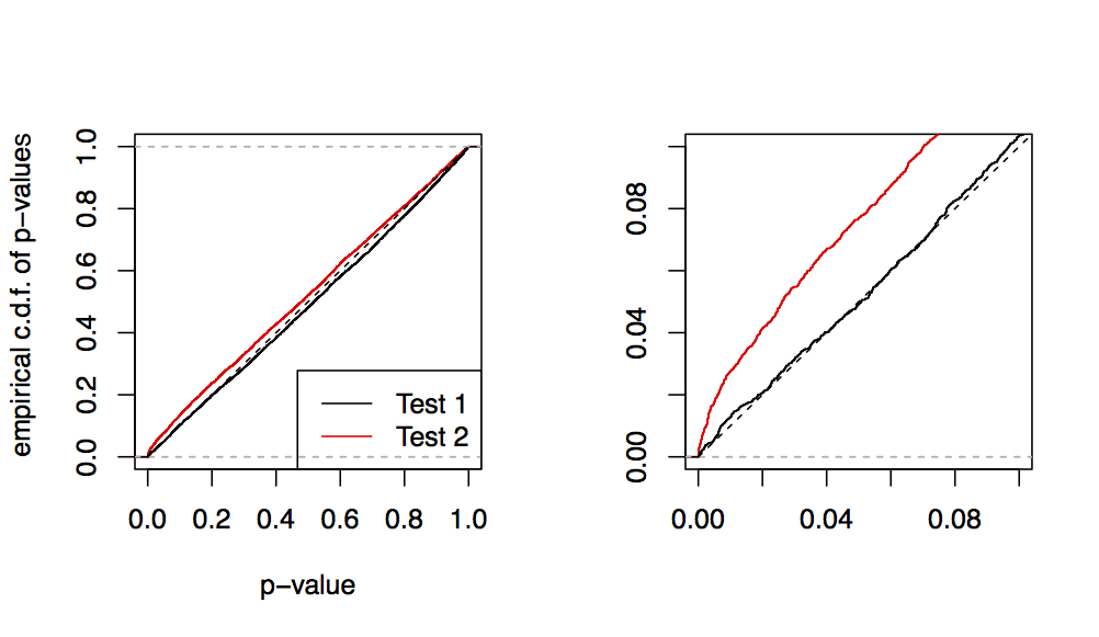
Figure 1: [left] Empirical c.d.f. of p-values of $T_{1}$ and $T_{2}$ under $H_{0}:\theta_{0}=(2,1.4)^{\top}$; 5000 replications with $N=250$, $n=817$. [right] Zoom-in on the region of interest: p-values smaller than 0.1.

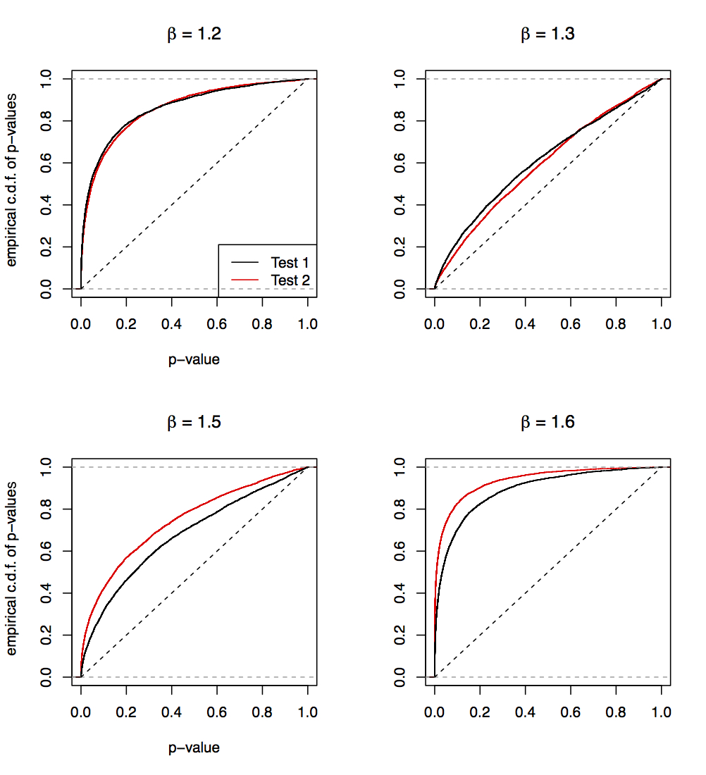
Figure 2: Empirical c.d.f. of p-values of $T_{1}$ and $T_{2}$ for testing $H_{0}:\theta_{0}=(2,1.4)^{\top}$ under several alternatives of the form $\theta=(2,\beta)^{\top}$; 5000 replications with $N=250$, $n=817$.

Signif. level	5%					10%
$\beta$	1.2	1.3	1.4	1.5	1.6	1.2	1.3	1.4	1.5	1.6
$T_{1}$	.532	.137	.049	.208	.576	.653	.223	.103	.315	.702
$T_{2}$	.500	.104	.077	.313	.735	.634	.184	.134	.421	.827

Table 1: Numerical results of the comparison for testing procedure $H_{0}\colon\theta=(2,1.4)^{\top}$ at significance level 5% and 10% . The column for $\beta=1.4$ provides the empirical size.

The above simulations (Fig. 1 and 2, Table 1) refer to the case of independent individual processes $\{X_{i}(t)\}$. There are no theoretical results for the parametric test $T_{2}$, when AR(1) series are dependent. Although the nonparametric test $T_{1}$ is valid for the latter case, one may expect that the presence of the common shock component in the panel data in (3.2) has a negative effect on the test performance for short series. To illustrate this effect, we simulate 5000 panels with AR(1) processes $\{X_{i}(t)\}$ driven by dependent shocks in (3.2) with $b_{i}=b$, $c_{i}=(1-b^{2})^{1/2}$. As previously, we choose $\theta_{0}=(2,1.4)^{\top}$, $N=250$, $n=817$ and we fix $\theta=(2,1.4)^{\top}$ to evaluate the empirical size of $T_{1}$. Fig. 3 [left] presents the graphs of the empirical c.d.f.’s of the p-values of $T_{1}$ for $b=1$, $b=0.6$ and $b=0$, the latter corresponding to independent individual processes as in Fig. 1. We see that the size of the test worsens when $b$ increases, particularly when $b=1$ and the individual processes are all driven by the same common noise. To overcome the last effect, the sample length $n$ of each series in the panel may be increased as in Fig. 3 [right], where the choice of $n=5500$ and $b=1$ shows a much better performance of $T_{1}$ under the null hypothesis $\theta=\theta_{0}=(2,1.4)^{\top}$ and the alternative ($\theta=(2,1.5)^{\top}$ and $\theta=(2,1.6)^{\top}$) scenarios.

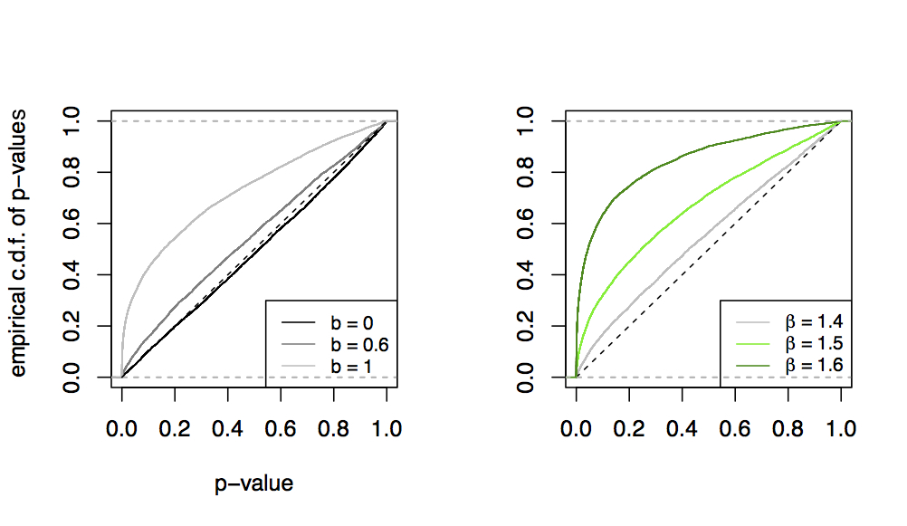
Figure 3: [left] Empirical c.d.f. of p-values of $T_{1}$ under $H_{0}\colon\theta_{0}=(2,1.4)^{\top}$ for different dependence structure between AR(1) series : $b_{i}=b$ and $c_{i}=\sqrt{1-b^{2}}$ and $N=250$, $n=817$. [right] Empirical c.d.f. of p-values of $T_{1}$ for testing $H_{0}:\theta_{0}=(2,1.4)^{\top}$. AR(1) series are driven by common innovations, i.e., $b_{i}=1$, $c_{i}=0$, for $\theta=(2,\beta)^{\top}$; 5000 replications with $N=250$, $n=5500$.

In conclusion,

1. We do not observe an important loss of the power for the nonparametric KS test $T_{1}$ compared to the parametric approach.

2. The KS test $T_{1}$ does not require to choose any tuning parameter contrary to the test $T_{2}$.

3. One can use the KS test $T_{1}$ under weaker assumptions on AR(1) innovations. We only impose moment conditions. The dependence between the series is allowed by (3.2).

7 Appendix: some proofs and auxiliary lemmas

We use the following martingale moment inequality.

Lemma 7.1

Let $p>1$ and $\{\xi_{j},j\geq 1\}$ be a martingale difference sequence: $\mathrm{E}[\xi_{j}|\xi_{1},\ldots,\xi_{j-1}]=0$, $j=2,3,\ldots$ with $\mathrm{E}|\xi_{j}|^{p}<\infty$. Then there exists a constant $C_{p}<\infty$ depending only on $p$ and such that

$$\mathrm{E}\Big{|}\sum_{j=1}^{\infty}\xi_{j}\Big{|}^{p}\ \leq\ C_{p}\begin{cases}\sum_{j=1}^{\infty}\mathrm{E}|\xi_{j}|^{p},&1<p\leq 2,\\ \big{(}\sum_{j=1}^{\infty}(\mathrm{E}|\xi_{j}|^{p})^{2/p}\big{)}^{p/2},&p>2.\end{cases}$$ (7.1)

For $1<p\leq 2$, inequality (7.1) is known as von Bahr and Esséen inequality, see [21], and for $p>2$, it is a consequence of the Burkholder and Rosenthal inequality ([3, 16], see also [8, Lemma 2.5.2]).

Proof of Proposition 2.1. Since $\widehat{a}_{n}$ in (2.5) is invariant w.r.t. a scale factor of innovations $\{\zeta(t)\}$, w.l.g. we can assume $b^{2}+c^{2}=1$ and $\mathrm{E}\zeta^{2}(0)=1,$ $\mathrm{E}|\zeta(0)|^{2p}<\infty$. Then $\widehat{a}_{n}-a=\sum_{i=1}^{3}\delta_{ni}$, where

$$\delta_{n1} := -\frac{aX^{2}(n)}{\sum_{t=1}^{n}X^{2}(t)-n(\bar{X}_{n})^{2}},\quad\delta_{n2}\ :=\ \frac{\sum_{t=1}^{n-1}X(t)\zeta(t+1)}{\sum_{t=1}^{n}X^{2}(t)-n(\bar{X}_{n})^{2}},$$

$$\delta_{n3} := \frac{\bar{X}_{n}(X(1)+X(n))-(\bar{X}_{n})^{2}(1+n(1-a))}{\sum_{t=1}^{n}X^{2}(t)-n(\bar{X}_{n})^{2}}.$$

The statement of the proposition follows from

$$\Pr(|\delta_{ni}|>\gamma)\leq C(n^{-1}+n^{-(p/2)\wedge(p-1)}\gamma^{-p})\qquad(0<\gamma<1,\,i=1,2,3).$$ (7.2)

To show (7.2) for $i=1$, note that $\delta_{n1}=L_{n}/(n+D_{n})$, where $L_{n}:=-a(1-a^{2})X^{2}(n)$ and $D_{n}=D_{n1}-D_{n2}$, $D_{n1}:=\sum_{t=1}^{n}((1-a^{2})X^{2}(t)-1)$, $D_{n2}:=n(1-a^{2})(\bar{X}_{n})^{2}$. We have $\Pr(|\delta_{n1}|>\gamma)\leq\Pr(|D_{n}|>n/2)+\Pr(|L_{n}|>n\gamma/2)$. Thus, (7.2) for $i=1$ follows from

$$\mathrm{E}|D_{n1}|^{p\wedge 2} \leq Cn,\qquad\mathrm{E}|D_{n2}|\ \leq\ C\qquad\text{and}\qquad\mathrm{E}|L_{n}|^{p}\ \leq\ C.$$ (7.3)

Consider the first relation in (7.3). Clearly, it suffices to prove it for $1<p\leq 2$ only. We have $D_{n1}=2D^{\prime}_{n1}+D^{\prime\prime}_{n1}$, where

$$D^{\prime}_{n1} := (1-a^{2})\sum_{s_{2}<s_{1}\leq n}\sum_{t=1\vee s_{1}}^{n}a^{2(t-s_{1})}a^{s_{1}-s_{2}}\zeta(s_{1})\zeta(s_{2}),$$

$$D^{\prime\prime}_{n1} := (1-a^{2})\sum_{s\leq n}\sum_{t=1\vee s}^{n}a^{2(t-s)}(\zeta^{2}(s)-1).$$

We will use the following elementary inequality: for any $-1\leq a\leq 1,n\geq 1,s\leq n$

$$\alpha_{n}(s)\ :=\ (1-a^{2})\sum_{t=1\vee s}^{n}a^{2(t-s)} = \begin{cases}a^{2(1-s)}(1-a^{2n}),&s\leq 0,\\ 1-a^{2(n+1-s)},&1\leq s\leq n\end{cases}$$ (7.4)

$$\leq C\begin{cases}a^{-2s}\min(1,2n(1-|a|)),&s\leq 0,\\ 1,&1\leq s\leq n.\end{cases}$$

Using the independence of $\{\zeta(s)\}$ and $a$ and inequality (7.1) (twice) for $1<p\leq 2$ we obtain

$$\mathrm{E}|D^{\prime}_{n1}|^{p} = \mathrm{E}\big{|}\sum_{s_{1}\leq n}\alpha_{n}(s_{1})\zeta(s_{1})\sum_{s_{2}<s_{1}}a^{s_{1}-s_{2}}\zeta(s_{2})\big{|}^{p}$$

$$\leq C\mathrm{E}\sum_{s_{1}\leq n}\big{|}\alpha_{n}(s_{1})\zeta(s_{1})\sum_{s_{2}<s_{1}}a^{s_{1}-s_{2}}\zeta(s_{2})\big{|}^{p}$$

$$\leq C\mathrm{E}\sum_{s_{1}\leq n}|\alpha_{n}(s_{1})|^{p}\sum_{s_{2}<s_{1}}|a|^{p(s_{1}-s_{2})}$$

$$\leq C\mathrm{E}(1-|a|)^{-1}\sum_{s\leq n}|\alpha_{n}(s)|^{p}\ \leq\ Cn$$

since $\mathrm{E}(1-|a|)^{-1}<\infty$ (see (2.3)) and $\sum_{s\leq n}|\alpha_{n}(s)|^{p}\leq Cn$ follows from (7.4). Similarly, since $\{\zeta^{2}(s)-1,\,s\leq n\}$ form a martingale difference sequence,

$$\mathrm{E}|D^{\prime\prime}_{n1}|^{p} \leq C\mathrm{E}\sum_{s\leq n}|\alpha_{n}(s)|^{p}\ \leq\ Cn,$$

proving the first inequality (7.3). The second inequality in (7.3) follows by noting that $n\bar{X}_{n}=\sum_{s\leq n}(\sum_{t=1\vee s}^{n}a^{t-s})\zeta(s)$ and

$$(1-a^{2})\mathrm{E}[(n\bar{X}_{n})^{2}|a]=a^{2}\Big{(}\frac{1-a^{n}}{1-a}\Big{)}^{2}+(1-a^{2})\sum_{s=1}^{n}\Big{(}\frac{1-a^{s}}{1-a}\Big{)}^{2}\leq\frac{Cn}{1-a}.$$

Consider the last inequality in (7.3). We have $|L_{n}|\leq|2L^{\prime}_{n}+L^{\prime\prime}_{n}+1|$, where

$$L^{\prime}_{n} := (1-a^{2})\sum_{s_{2}<s_{1}\leq n}a^{2(n-s_{1})}a^{s_{1}-s_{2}}\zeta(s_{1})\zeta(s_{2}),\qquad L^{\prime\prime}_{n}\ :=\ (1-a^{2})\sum_{s\leq n}a^{2(n-s)}(\zeta^{2}(s)-1).$$

We use Lemma 7.1, as above. Let $1\leq p\leq 2$. Then $\mathrm{E}|L^{\prime\prime}_{n}|^{p}\leq C\mathrm{E}\sum_{s\leq n}\{(1-a^{2})a^{-2(n-s)}\}^{p}\leq C$ and $\mathrm{E}|L^{\prime}_{n}|^{p}\leq C\mathrm{E}\sum_{s_{2}<s_{1}\leq n}\{(1-a^{2})|a|^{2(n-s_{1})}|a|^{s_{1}-s_{2}}\}^{p}\leq C\mathrm{E}(1-|a|)^{p-2}\leq C$. Next, let $p\geq 2$. Then $\mathrm{E}|L^{\prime\prime}_{n}|^{p}\leq C\mathrm{E}\{\sum_{s\leq n}|(1-a^{2})a^{2(n-s)}|^{2}\}^{p/2}\leq C$ and $\mathrm{E}|L^{\prime}_{n}|^{p}\leq C\mathrm{E}(1-a^{2})^{p}\{\sum_{s_{2}<s_{1}\leq n}a^{4(n-s_{1})}a^{2(s_{1}-s_{2})}\}^{p/2}\leq C$, proving (7.3) and hence (7.2) for $i=1$.

Consider (7.2) for $i=2$. We have $\delta_{n2}=R_{n}/(n+D_{n})$, where $R_{n}:=(1-a^{2})\sum_{t=1}^{n-1}X(t)\zeta(t+1)$ and $D_{n}$ is the same as in (7.3). Then $\Pr(|\delta_{n2}|>\gamma)\leq\Pr(|R_{n}|>n\gamma/2)+\Pr(|D_{n}|>n/2)$, where

$$\Pr(|D_{n}|>n/2) \leq (n/4)^{-(p\wedge 2)}\mathrm{E}|D_{n1}|^{p\wedge 2}+(n/4)^{-1}\mathrm{E}|D_{n2}|$$ (7.5)

$$\leq C\begin{cases}n^{-(p-1)},&1<p\leq 2,\\ n^{-1},&p>2,\end{cases}$$

according to (7.3). Therefore (7.2) for $i=2$ follows from

$$\mathrm{E}|R_{n}|^{p}\leq C\begin{cases}n,&1<p\leq 2,\\ n^{p/2},&p>2.\end{cases}$$ (7.6)

Since $R_{n}=(1-a^{2})\sum_{s\leq n-1}\zeta(s)\sum_{t=1\vee s}^{n-1}a^{t-s}\zeta(t+1)$ is a sum of martingale differences, by inequality (7.1) with $1<p\leq 2$ we obtain

$$\mathrm{E}|R_{n}|^{p} \leq C\mathrm{E}\sum_{s\leq n-1}\big{|}(1-a^{2})\zeta(s)\sum_{t=1\vee s}^{n-1}a^{t-s}\zeta(t+1)\big{|}^{p}$$

$$\leq C\mathrm{E}|1-a^{2}|^{p}\sum_{s\leq n-1}\sum_{t=1\vee s}^{n-1}|a|^{p(t-s)}$$

$$\leq C\mathrm{E}|1-a^{2}|^{p}\big{(}\sum_{s\leq 0}|a|^{-ps}\sum_{t=1}^{n-1}|a|^{pt}+\sum_{s=1}^{n-1}\sum_{t=s}^{n-1}|a|^{p(t-s)}\big{)}$$

$$\leq C\mathrm{E}|1-a^{2}|^{p}\big{\{}(1-|a|^{p})^{-2}+n(1-|a|^{p})^{-1}\big{\}}\ \leq Cn,$$

proving (7.6) for $p\leq 2$. Similarly, using (7.1) with $p>2$ we get

$$\mathrm{E}|R_{n}|^{p} = \mathrm{E}\Big{[}|1-a^{2}|^{p}\mathrm{E}\big{[}|\sum_{s\leq n-1}\zeta(s)\sum_{t=1\vee s}^{n-1}a^{t-s}\zeta(t+1)|^{p}\big{|}a\big{]}\Big{]}$$

$$\leq C\mathrm{E}\Big{[}|1-a^{2}|^{p}\big{\{}\sum_{s\leq n-1}\big{(}\mathrm{E}\big{[}|\zeta(s)\sum_{t=1\vee s}^{n-1}a^{t-s}\zeta(t+1)|^{p}\big{|}a\big{]}\big{)}^{2/p}\big{\}}^{p/2}\Big{]}$$

$$\leq C\mathrm{E}|1-a^{2}|^{p}\big{\{}\sum_{s\leq n-1}\sum_{t=1\vee s}^{n-1}a^{2(t-s)}\big{\}}^{p/2}$$

$$\leq C\mathrm{E}|1-a^{2}|^{p}\big{\{}\sum_{s\leq 0}a^{-2s}\sum_{t=1}^{n-1}a^{2t}+\sum_{s=1}^{n-1}\sum_{t=s}^{n-1}a^{2(t-s)}\big{\}}^{p/2}$$

$$\leq C\mathrm{E}|1-a^{2}|^{p}\big{\{}(1-a^{2})^{-2}+n(1-a^{2})^{-1}\big{\}}^{p/2}\ \leq\ Cn^{p/2},$$

proving (7.6) and (7.2) for $i=2$.

It remains to prove (7.2) for $i=3$. Similarly as above, $\Pr(|\delta_{n3}|>\gamma)\leq\Pr(|Q_{n}|>n\gamma/2)+\Pr(|D_{n}|>n/2)$, where $Q_{n}:=(1-a^{2})\{\bar{X}_{n}(X(1)+X(n))-(\bar{X}_{n})^{2}(1+n(1-a))\}$ and $D_{n}$ is evaluated in (7.5). Thus, (7.2) for $i=3$ follows from (7.5) and

$$\mathrm{E}|Q_{n}|^{p}\ \leq\ C\{\mathrm{E}|(1-a^{2})X^{2}(n)|^{p}+\mathrm{E}|(1-a^{2})(\bar{X}_{n})^{2}|^{p}+n^{p}\mathrm{E}|(1-a)(1-a^{2})(\bar{X}_{n})^{2}|^{p}\}\ \leq\ C.$$ (7.7)

Since $n\bar{X}_{n}=\sum_{s\leq n}(\sum_{t=1\vee s}^{n}a^{t-s})\zeta(s)$, an application of the second inequality of (7.1) yields

$$\mathrm{E}[|n\bar{X}_{n}|^{2p}|a]\leq C\Big{(}\frac{(1-a^{n})^{2}}{(1-a^{2})(1-a)^{2}}+\sum_{s=1}^{n}\Big{(}\frac{1-a^{s}}{1-a}\Big{)}^{2}\Big{)}^{p}.$$

Using $1-a^{n}\leq 1\wedge(n(1-a))$ we obtain $\mathrm{E}|(1-a)(1-a^{2})(\bar{X}_{n})^{2}|^{p}\leq Cn^{-p}$ and $\mathrm{E}|(1-a^{2})(\bar{X}_{n})^{2}|^{p}\leq C\mathrm{E}(1-a)^{-1}n^{-1}$. Finally, $\mathrm{E}|(1-a^{2})X^{2}(n)|^{p}\leq C$ follows by the same arguments as $\mathrm{E}|L_{n}|^{p}\leq C$ (see (7.3)). This proves (7.7), thereby completing the proof of (7.2) and of the proposition, too. $\Box$

Let $a,a_{1},\ldots,a_{N}$ be i.i.d. r.v.s with d.f.  $G(x)=\Pr(a\leq x)$ supported by $[-1,1]$. Define $\widehat{G}_{N}(x):=N^{-1}\sum_{i=1}^{N}{\bf 1}(a_{i}\leq x)$, $U_{N}(x):=N^{1/2}(\widehat{G}_{N}(x)-G(x))$, $x\in\mathbb{R}$, and $\omega_{N}(\delta)$ (= the modulus of continuity of $U_{N}$) by

$$\omega_{N}(\delta)\ :=\ \sup_{0\leq y-x\leq\delta}|U_{N}(y)-U_{N}(x)|,\quad\delta>0.$$

Lemma 7.2

Assume that $G$ satisfies Assumption A₆. Then for all $\epsilon>0$,

$$\epsilon^{4}\Pr(\omega_{N}(\delta)>6\epsilon)\ \leq\ (3+3C)L_{G}\delta^{\varrho}+N^{-1},$$

where $C$ is a constant independent of $\epsilon,\,\delta,\,N$.

Proof. As in [2, p. 106, (13.17)] we have that

$$\mathrm{E}|U_{N}(y)-U_{N}(x)|^{2}|U_{N}(z)-U_{N}(y)|^{2} \leq 3\Pr(a\in(x,y])\Pr(a\in(y,z]),$$

$$\mathrm{E}|U_{N}(y)-U_{N}(x)|^{4} \leq 3\Pr(a\in(x,y])^{2}+N^{-1}\Pr(a\in(x,y])$$

for $-1\leq x\leq y\leq z\leq 1$, where the second inequality treats the 4th central moment of a binomial variable. Now fix $\delta>0$ and split $[-1,1]=\cup_{i}\Delta_{i}$, where $\Delta_{i}=[-1+i\delta,-1+(i+1)\delta]$, $i=0,1,\ldots,\lfloor 2/\delta\rfloor-1$, $\Delta_{\lfloor 2/\delta\rfloor}=[-1+\lfloor 2/\delta\rfloor\delta,1]$. According to [17, p. 49, Lemma 1], for all $\epsilon>0$,

$$\epsilon^{4}\Pr(\omega_{N}(\delta)>6\epsilon)\ \leq\ (3+3C)\max_{i}\Pr(a\in\Delta_{i})+N^{-1},$$

where $C$ is a constant independent of $\epsilon,\,\delta,\,N$. Lemma follows from Assumption A₆ on the d.f. $G$ of the r.v. $a$. $\Box$

Note that if we take $\delta=\delta_{N}=o(1)$, we then get $\Pr(\omega_{N}(\delta)>\epsilon)\to 0$ as $N\to\infty$.

Lemma 7.3

Let $\widehat{a}_{1,n},\widehat{a}_{2,n}$ be given in (3.3) under Assumptions A₁–A₆ with $\varrho=1$. Then for all $\gamma\in(0,1)$ and $n\geq 1$, it holds

$$\sup_{x,y\in[-1,1]}|\Pr(\widehat{a}_{1,n}\leq x,\,\widehat{a}_{2,n}\leq y)-\Pr(\widehat{a}_{1,n}\leq x)\Pr(\widehat{a}_{2,n}\leq y)|\ =\ O(n^{-((p/2)\wedge(p-1))/(1+p)}).$$

Proof. Define $\delta_{i,n}:=\widehat{a}_{i,n}-a_{i}$, $i=1,2$. For $\gamma\in(0,1)$, we have

$$\Pr(|\delta_{1,n}|>\gamma\,\text{or}\,|\delta_{2,n}|>\gamma)\ \leq\ \Pr(|\delta_{1,n}|>\gamma)+\Pr(|\delta_{2,n}|>\gamma)\ \leq\ C(n^{-((p/2)\wedge(p-1))}\gamma^{-p}+n^{-1})$$

by Proposition 2.1. Consider now

$$\Pr(\widehat{a}_{1,n}\leq x,\,\widehat{a}_{2,n}\leq y) = \Pr(a_{1}+\delta_{1,n}\leq x,\,a_{2}+\delta_{2,n}\leq y)$$

$$\leq \Pr(a_{1}+\delta_{1,n}\leq x,\,a_{2}+\delta_{2,n}\leq y,\,|\delta_{1,n}|\leq\gamma,\,|\delta_{2,n}|\leq\gamma)+\Pr(|\delta_{1,n}|>\gamma\,\text{or}\,|\delta_{2,n}|>\gamma).$$

Then

$$\Pr(a_{1}+\delta_{1,n}\leq x,\,a_{2}+\delta_{2,n}\leq y,\,|\delta_{1,n}|\leq\gamma,\,|\delta_{2,n}|\leq\gamma) \leq \Pr(a_{1}\leq x+\gamma,\,a_{2}\leq y+\gamma,\,|\delta_{1,n}|\leq\gamma,\,|\delta_{2,n}|\leq\gamma)$$

$$\leq G(x+\gamma)G(y+\gamma)$$

and

$$\Pr(a_{1}+\delta_{1,n}\leq x,\,a_{2}+\delta_{2,n}\leq y,\,|\delta_{1,n}|\leq\gamma,\,|\delta_{2,n}|\leq\gamma) \geq \Pr(a_{1}\leq x-\gamma,\,a_{2}\leq y-\gamma,|\delta_{1,n}|\leq\gamma,\,|\delta_{2,n}|\leq\gamma)$$

$$\geq G(x-\gamma)G(y-\gamma)-\Pr(|\delta_{1,n}|>\gamma\,\text{or}\,|\delta_{2,n}|>\gamma).$$

From (2.6) we obtain

$$|G(x\pm\gamma)G(y\pm\gamma)-G(x)G(y)|\ =\ |(G(x)+O(\gamma))(G(y)+O(\gamma))-G(x)G(y)|\ \leq\ C\gamma.$$

Hence,

$$|\Pr(a_{1}\leq x,\,a_{2}\leq y)-G(x)G(y)|\ \leq\ C(\gamma+n^{-1}+n^{-((p/2)\wedge(p-1))}\gamma^{-p}).$$ (7.8)

In a similar way,

$$|\Pr(a_{1}\leq x)\Pr(a_{2}\leq y)-G(x)G(y)|\ \leq\ C(\gamma+n^{-1}+n^{-((p/2)\wedge(p-1))}\gamma^{-p}).$$ (7.9)

By (7.8), (7.9), the proof of the lemma is complete with $\gamma=\gamma_{n}=o(1)$, which satisfies $\gamma_{n}\sim n^{-(p/2)\wedge(p-1)}\gamma^{-p}_{n}$. $\Box$

References

[1]
J. Beran, M. Schützner, and S. Ghosh.
From short to long memory: Aggregation and estimation.
Computational Statistics and Data Analysis, 54:2432–2442,
2010.
[2]
P. Billingsley.
Convergence of Probability Measures.
Wiley, New York, 1968.
[3]
D. L. Burkholder.
Distribution function inequalities for martingales.
Annals of Probability, 1:19–42, 1973.
[4]
D. Celov, R. Leipus, and A. Philippe.
Time series aggregation, disaggregation and long memory.
Lithuanian Mathematical Journal, 47:379–393, 2007.
[5]
D. Celov, R. Leipus, and A. Philippe.
Asymptotic normality of the mixture density estimator in a
disaggregation scheme.
Journal of Nonparametric Statistics, 22:425–442, 2010.
[6]
T. T. Chong.
The polynomial aggregated AR(1) model.
Econometrics Journal, 9:98–122, 2006.
[7]
J. Durbin.
Weak convergence of the sample distribution function when parameters
are estimated.
Annals of Statistics, 1:279–290, 1973.
[8]
L. Giraitis, H. L. Koul, and D. Surgailis.
Large Sample Inference for Long Memory Processes.
Imperial College Press, London, 2012.
[9]
C. W. J. Granger.
Long memory relationship and the aggregation of dynamic models.
Journal of Econometrics, 14:227–238, 1980.
[10]
L. Horváth and R. Leipus.
Effect of aggregation on estimators in AR(1) sequence.
TEST, 18:546–567, 2009.
[11]
M. Jirak.
Limit theorems for aggregated linear processes.
Advances in Applied Probability, 45:520–544, 2013.
[12]
R. Leipus, G. Oppenheim, A. Philippe, and M.-C. Viano.
Orthogonal series density estimation in a disaggregation scheme.
Journal of Statistical Planning and Inference, 136:2547–2571,
2006.
[13]
E. Parzen.
On estimation of a probability density function and mode.
Annals of Mathematical Statistics, 33:1065–1076, 1962.
[14]
D. Puplinskaitė and D. Surgailis.
Aggregation of random coefficient AR(1) process with infinite
variance and common innovations.
Lithuanian Mathematical Journal, 49:446–463, 2009.
[15]
P. M. Robinson.
Statistical inference for a random coefficient autoregressive model.
Scandinavian Journal of Statistics, 5:163–168, 1978.
[16]
H. P. Rosenthal.
On the subspaces of spanned by sequences of
independent random variables.
Israel Journal of Mathematics, 8:273–303, 1970.
[17]
G.R. Shorack and J.A. Wellner.
Empirical Processes with Applications to Statistics.
Wiley, New York, 1986.
[18]
W. Stute, W. Gonzáles-Manteiga, and M. Presedo-Quindimil.
Bootstrap based goodness-of-fit tests.
Metrika, 40:243–256, 1993.
[19]
G. Szűcs.
Parametric bootstrap tests for continuous and discrete distributions.
Metrika, 67:63–68, 2008.
[20]
A.W. van der Vaart.
Asymptotic Statistics.
Cambridge University Press, 2000.
[21]
B. von Bahr and C.-G. Esséen.
Inequalities for the th absolute moment of a sum of random
variables, .
Annals of Mathematical Statistics, 36:299–303, 1965.