Qubit lattice coherence induced by electromagnetic pulses in superconducting metamaterials

Abstract

Quantum bits (qubits) are at the heart of quantum information processing schemes. Currently, solid-state qubits, and in particular the superconducting ones, seem to satisfy the requirements for being the building blocks of viable quantum computers, since they exhibit relatively long coherence times, extremely low dissipation, and scalability. The possibility of achieving quantum coherence in macroscopic circuits comprising Josephson junctions, envisioned by Legett in the 1980’s, was demonstrated for the first time in a charge qubit; since then, the exploitation of macroscopic quantum effects in low-capacitance Josephson junction circuits allowed for the realization of several kinds of superconducting qubits. Furthermore, coupling between qubits has been successfully achieved that was followed by the construction of multiple-qubit logic gates and the implementation of several algorithms. Here it is demonstrated that induced qubit lattice coherence as well as two remarkable quantum coherent optical phenomena, i.e., self-induced transparency and Dicke-type superradiance, may occur during light-pulse propagation in quantum metamaterials comprising superconducting charge qubits. The generated qubit lattice pulse forms a compound ”quantum breather” that propagates in synchrony with the electromagnetic pulse. The experimental confirmation of such effects in superconducting quantum metamaterials may open a new pathway to potentially powerful quantum computing.

Introduction

Quantum simulation, that holds promises of solving particular problems exponentially faster than any classical computer, is a rapidly expanding field of research Devoret2013 ; Paraoanu2014 ; Georgescu2014 . The information in quantum computers is stored in quantum bits or qubits, which have found several physical realizations; quantum simulators have been nowadays realized and/or proposed that employ trapped ions Blatt2012 , ultracold quantum gases Bloch2012 , photonic systems Aspuru-Guzik2012 , quantum dots Press2008 , and superconducting circuits Houck2012 ; Schmidt2013 ; Devoret2013 . Solid state devices, and in particular those relying on the Josephson effect Josephson1962 , are gaining ground as preferable elementary units (qubits) of quantum simulators since they exhibit relatively long coherence times and extremely low dissipation Wendin2007 . Several variants of Josephson qubits that utilize either charge or flux or phase degrees of freedom have been proposed for implementing a working quantum computer; the recently anounced, commercially available quantum computer with more than $1000$ ’ superconducting qubit CPU, known as D-Wave 2X^TM (the upgrade of D-Wave Two^TM with $512$ qubits CPU), is clearly a major advancement in this direction. A single superconducting charge qubit (SCQ) Pashkin2009 at milikelvin temperatures behaves effectively as an artificial two-level ”atom” in which two states, the ground and the first excited ones, are coherently superposed by Josephson coupling. When coupled to an electromagnetic (EM) vector potential, a single SCQ does behave, with respect to the scattering of EM waves, as an atom in space. Indeed, a “single-atom laser” has been realized with an SCQ coupled to a transmission line resonator (“cavity”) Astafiev2007 . Thus, it would be anticipated that a periodic structure of SCQs demonstrates the properties of a transparent material, at least in a particular frequency band. The idea of building materials comprising artificial ”atoms” with engineered properties, i.e., metamaterials, and in particular superconducting ones Jung2014 , is currently under active development. Superconducting quantum metamaterials (SCQMMs) comprising a large number of qubits could hopefully maintain quantum coherence for times long enough to reveal new, exotic collective properties. The first SCQMM that was only recently implemented comprises $20$ flux qubits arranged in a double chain geometry Macha2014 . Furthermore, lasing in the microwave range has been demonstrated theoretically to be triggered in an SCQMM initialized in an easily reachable factorized state Asai2015 .

Results

Superconducting Quantum Metamaterial Model

Consider an infinite, one-dimensional (1D) periodic SCQ array placed in a transmission line (TL) consisting of two superconducting strips of infinite length Rakhmanov2008 ; Shvetsov2013 (Figure 1a and b); each SCQ, in the form of a tiny superconducting island, is connected to each bank of the TL by a Josephson junction (JJ). The control circuitry for each individual SCQ (Figure 1c), consisting of a gate voltage source $V_{g}$ coupled to it through a gate capacitor $C_{g}$, allows for local control of the SCQMM by altering independently the state of each SCQ Zagoskin2011 . The SCQs exploit the nonlinearity of the Josephson effect and the large charging energy resulting from nanofabrication to create artificial mesoscopic two-level systems. A propagating EM field in the superconducting TL gives rise to nontrivial interactions between the SCQs, that are mediated by its photons vanLoo2013 . Those interactions are of fundamental importance in quantum optics, quantum simulations, and quantum information processing, as well. In what follows, it is demonstrated theoretically that self-induced transparency McCall1967 and Dicke-type superradiance (collective spontaneous emission) Dicke1954 occur for weak EM fields in that SCQMM structure; the occurence of the former or the latter effect solely depends on the initial state of the SCQ subsystem. Most importantly, self-induced transparent (SIT) or superradiant (SRD) pulses induce quantum coherence effects in the qubit subsystem. In superradiance (resp. self-induced transparency), the initial conditions correspond to a state where the SCQs are all in their excited (resp. ground) state; an extended system exhibiting SRD or SIT effects is often called a coherent amlpifier or attenuator, respectively. These fundamental quantum coherent prosesses have been investigated extensively in connection to one- and two-photon resonant two-level systems. Superradiant effects have been actually observed recently in two-level systems formed by quantum dot arrays Scheibner2007 and spin-orbit coupled Bose-Einstein condensates Hamner2014 ; the latter system features the coupling between momentum states and the collective atomic spin which is analogous to that between the EM field and the atomic spin in the original Dicke model. These results suggest that quantum dots and the atoms in the Bose-Einstein condensate can radiatively interact over long distances. The experimental confirmation of SIT and SRD in extended SCQMM structures may open a new pathway to potentially powerful quantum computing. As a consequence of these effects, the value of the speed of either an SIT or SRD propagating pulse in a SCQMM structure can in principle be engineered through the SCQ parameters Cornell2001 , which is not possible in ordinary resonant media. From a technological viewpoint, an EM (light) pulse can be regarded as a ”bit” of optical information; its slowing down, or even its complete halting for a certain time interval, may be used for data storage in a quantum computer.

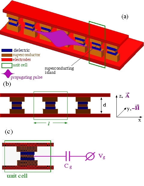
Figure 1: Schematic drawing of a charge qubit superconducting quantum metamaterial (SCQMM). (a) The SCQMM comprising an infinite chain of identical charge qubits in a superconducting transmission line. Each qubit consists of a superconducting island that is connected to the electrodes of the transmission line through two Josephson junctions, formed in the regions of the dielectric layers (blue). The propagating electromagnetic vector potential pulse is also shown schematically out of scale. (b) The side view of the SCQMM in which the relevant geometrical parameters and the field orientations are indicated. (c) A unit cell of the superconducting quantum metamaterial which also shows the control circuitry of the charge qubit, consisting of a gate potential $V_{g}$ applied to it through the gate capacitor $C_{g}$.

In the following, the essential building blocks of the SCQMM model are summarized in a self-contained manner, yet omitting unnecessary calculational details which are presented in the Supplementary Information. The energy per unit cell of the SCQMM structure lying along the $x-$direction, when coupled to an EM vector potential $\vec{A}=A_{z}(x,t)\hat{z}$, can be readily written as Rakhmanov2008 ; Shvetsov2013

$$H=\sum_{n}\left\{\left[\dot{\varphi}^{2}_{n}-2\cos\varphi_{n}\right]+\left[\dot{\alpha}^{2}_{n}+\beta^{2}(\alpha_{n+1}-\alpha_{n})^{2}\right]\right.$$

$$\left.+\left[2\cos\varphi_{n}(1-\cos\alpha_{n})\right]\right\},$$ (1)

in units of the Josephson energy $E_{J}=\Phi_{0}I_{c}/(2\pi C)$, with $\Phi_{0}$, $I_{c}$ and $C$ being the magnetic flux quantum, the critical current of the JJ, and the capacitance of the JJ, respectively. In equation (Superconducting Quantum Metamaterial Model), $\varphi_{n}$ is the superconducting phase on the $n$th island, $\beta=(8\pi dE_{J})^{-1/2}(\Phi_{0}/2\pi)$, with $d$ being the separation between the electrodes of the superconducting TL, and the overdots denote differentiation with respect to the temporal variable $t$. Assuming EM fields with wavelengths $\lambda>>\ell,d$, with $\ell$ being the distance between neighboring qubits, the EM potential is approximately constant within a unit cell, so that in the centre of the $n$th unit cell $A_{z}(x,t)\simeq A_{z,n}(t)$. In terms of the discretized EM potential $A_{z,n}(t)$, the normalized gauge term is $a_{n}=2\pi dA_{x,n}/\Phi_{0}$. The classical energy expression equation (Superconducting Quantum Metamaterial Model) provides a minimal modelling approach for the system under consideration; the three angular brackets in that equation correspond to the energies of the SCQ subsystem, the EM field inside the TL electrodes, and their interaction, respectively. The latter results from the requirement for gauge-invariance of each Josephson phase.

Second Quantization and Reduction to Maxwell-Bloch Equations

The quantization of the SCQ subsystem requires the replacement of the classical variables $\varphi_{n}$ and $\dot{\varphi}_{n}$ by the corresponding quantum operators $\hat{\varphi}_{n}$ and $-i({\partial}/{\partial\hat{\varphi}_{n}})$, respectively. While the EM field is treated classically, the SCQs are regarded as two-level systems, so that only the two lowest energy states are retained; under these considerations, the second-quantized Hamiltonian corresponding to equation (Superconducting Quantum Metamaterial Model) is

$$H=\sum_{n}\sum_{p}E_{p}(n)a^{\dagger}_{n,p}a_{n,p}+\sum_{n}\left[\dot{\alpha}^{2}_{n}+\beta^{2}(\alpha_{n+1}-\alpha_{n})^{2}\right]$$

$$+4\sum_{n}\sum_{p,p^{\prime}}V_{p,p^{\prime}}(n)a^{\dagger}_{n,p}a_{n,p^{\prime}}\sin^{2}\frac{\alpha_{n}}{2},~{}~{}~{}~{}~{}$$ (2)

where $p,p^{\prime}=0,1$, $E_{0}$ and $E_{1}$ are the energy eigenvalues of the ground and the excited state, respectively, the operator $a^{\dagger}_{n,p}$ ($a_{n,p}$) excites (de-excites) the $n$th SCQ from the ground to the excited (from the excited to the ground) state, and $V_{p,p^{\prime}}=\int d\varphi\Xi^{*}_{p}(\varphi)\cos\varphi\Xi_{p}(\varphi)$ are the matrix elements of the effective SCQ-EM field interaction. The basis states $\Xi_{p}$ can be obtained by solving the single-SCQ Schrödinger equation $(-{\partial^{2}}/{\partial\varphi^{2}}-E_{p}+2\cos\varphi)\Xi_{p}=0$. In general, each SCQ is in a superposition state of the form $|\Psi_{n}\rangle=\sum_{p}\Psi_{n,p}(t)a^{\dagger}_{n,p}|0\rangle$. The substitution of $|\Psi_{n}\rangle$ into the Schrödinger equation with the second-quantized Hamiltonian equation (Second Quantization and Reduction to Maxwell-Bloch Equations), and the introduction of the Bloch variables $R_{x}(n)=\Psi^{\star}_{n,1}\Psi_{n,0}+\Psi^{\star}_{n,0}\Psi_{n,1}$, $R_{y}(n)=i(\Psi^{\star}_{n,0}\Psi_{n,1}-\Psi^{\star}_{n,1}\Psi_{n,0})$, $R_{z}(n)=|\Psi_{n,1}|^{2}-|\Psi_{n,0}|^{2}$, provides the re-formulation of the problem into the Maxwell-Bloch (MB) equations

$$\dot{R}_{x}(n) =-\left[\Delta+8D\sin^{2}\frac{\alpha_{n}}{2}\right]R_{y}(n),$$ (3)

$$\dot{R}_{y}(n) =\left[\Delta+8D\sin^{2}\frac{\alpha_{n}}{2}\right]R_{x}(n)-8\mu\sin^{2}\frac{\alpha_{n}}{2}R_{z}(n),$$ (4)

$$\dot{R}_{z}(n) =+8\mu\sin^{2}\frac{\alpha_{n}}{2}R_{y}(n),$$ (5)

that are nonlinearly coupled to the resulting EM vector potential equation

$$\ddot{\alpha}_{n}+\left\{\Omega^{2}+\chi\left[\mu R_{x}(n)+DR_{z}(n)\right]\right\}\sin\alpha_{n}=\beta^{2}\delta a_{n},$$ (6)

where $\delta\alpha_{n}=\alpha_{n-1}-2\alpha_{n}+\alpha_{n+1}$, $D=(V_{11}-V_{00})/(2\chi)$, $\Omega^{2}=(V_{00}+V_{11})/2$, $\mu=V_{10}/\chi=V_{01}/\chi$, and $\Delta=\epsilon_{1}-\epsilon_{0}\equiv(E_{1}-E_{0})/\chi$, with $\chi=\hbar\omega_{J}/E_{J}$. In the earlier equations, the overdots denote differentiation with respect to the normalized time $t\rightarrow\omega_{J}t$, in which $\omega_{J}=eI_{c}/(\hbar C)$ is the Josephson frequency and $e$, $\hbar$ are the electron charge and the Planck’s constant devided by $2\pi$, respectively.

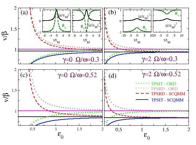
Figure 2: The velocity-amplitude relation in two-photon superradiant (TPSRD, amplifying) and two-photon self-induced transparent (TPSIT, absorbing) superconducting quantum metamaterials (SCQMMs) $\&$ quantum coherent pulse profiles. In all subfigures, the pulse velocity $v$ in units of $\beta$ as a function of the electromagnetic vector potential pulse amplitude $\varepsilon_{0}$ is plotted and compared with the corresponding curves for ordinary (atomic) amplifying and absorbing media (brown- and green-dotted curves, respectively). The horizontal magenta-solid (resp. black-solid) lines indicate the limiting velocity in ordinary amplifying and absorbing media, $v/\beta=1$ (resp. amplifying and absorbing SCQMMs, $v=c<\beta$). (a) $V_{00}=V_{11}=1$, $V_{01}=V_{10}=0.8$, $\chi=1/5$, $E_{1}-E_{0}=3$ ($\gamma=0$ and $\Omega/\omega=0.3$). Left Inset: The electromagnetic vector potential pulse envelop $(\varepsilon/\varepsilon_{M})^{2}$ and the population inversion function $R_{z}(n)$ profiles as a function of the slow variable $(\tau/\tau_{M}$ in a frame of reference that is moving with velocity $v$, for TPSIT (absorbing) SCQMMs. Right Inset: Same as in the left inset for TPSRD (amplifying) SCQMMs. (b) $V_{00}=0.6$, $V_{11}=1.4$, $V_{01}=V_{10}=0.8$, $\chi=1/5$, $E_{1}-E_{0}=3$ ($\gamma=2$ and $\Omega/\omega=0.3$). Left Inset: The electromagnetic vector potential pulse envelop $(\varepsilon/\varepsilon_{M})^{2}$ and the population inversion function $R_{z}(n)$ profiles as a function of the slow variable $(\tau/\tau_{M}$ in a frame of reference that is moving with velocity $v$, for TPSIT (absorbing) SCQMMs in the presence of relatively strong decoherence ($\gamma=2$). Right Inset: Same as in the left inset for TPSRD (amplifying) SCQMMs. (c) $V_{00}=V_{11}=3$, $V_{01}=V_{10}=0.8$, $\chi=1/5$, $E_{1}-E_{0}=3$ ($\gamma=0$ and $\Omega/\omega=0.52$). (d) $V_{00}=3$, $V_{11}=3.8$, $V_{01}=V_{10}=0.8$, $\chi=1/5$, $E_{1}-E_{0}=3$ ($\gamma=2$ and $\Omega/\omega=0.52$). The effect of non-zero decoherence ($\gamma\neq 0$) become apparent by direct comparison of a with b and c with d. The pulse velocity $v$ in SCQMMs saturates with increasing $\varepsilon_{0}$ to $v_{m}/\beta$, that can be significantly lower than that achieved in ordinary TPSIT and TPSRD media, i.e., $\beta$. The parameters of the SCQMM can be engineered to slow down the pulse velocity $v$ at the desired level for high enough amplitudes $\varepsilon_{0}$. Note that $v$ is also the velocity of the coherent qubit pulse.

Approximations and Analytical Solutions

For weak EM fields, the approximation $\sin\alpha_{n}\simeq\alpha_{n}$ can be safely used. Then, by taking the continuum limit $\alpha_{n}(t)\rightarrow\alpha(x,t)$ and $R_{i}(n;t)\rightarrow R_{i}(x;t)$ $(i=x,y,z)$ of equations (3-5) and (6), a set of simplified, yet still nonlinearly coupled equations is obtained, similar to those encountered in two-photon SIT in resonant media Belenov1969 . Further simplification can be achieved with the slowly varying envelope approximation (SVEA) by making for the EM vector potential the ansatz $\alpha(x,t)=\varepsilon(x,t)\cos\Psi(x,t)$, where $\Psi(x,t)=kx-\omega t+\phi(x,t)$ and $\varepsilon(x,t)$, $\phi(x,t)$ are the slowly varying pulse envelope and phase, respectively, with $\omega$ and $k=\pm\sqrt{\omega^{2}-\Omega^{2}}/\beta$ being the frequency of the carrier wave of the EM pulse and its wavenumber in the superconducting TL, respectively. In the absence of the SCQ chain the EM pulse is ”free” to propagate in the TL with speed $\beta$. At the same time, equations (3-5) for the Bloch vector components are transformed according to $R_{x}=r_{x}\cos(2\Psi)+r_{y}\sin(2\Psi)$, $R_{y}=r_{y}\cos(2\Psi)-r_{x}\sin(2\Psi)$, and $R_{z}=r_{z}$. Then, collecting the coefficients of $\sin\Psi$ and $\cos\Psi$ while neglecting the rapidly varying terms, and averaging over the phase $\Psi$, results in a set of truncated equations (see Supplementary Information). Further manipulation of the resulting equations and the enforcement of the two-photon resonance condition $\Delta=2\omega$, results in

$$\dot{\varepsilon}+c\varepsilon_{x}=-\chi\frac{\mu}{\Delta}\varepsilon r_{y},$$ (7)

$$\dot{\phi}+c\phi_{x}=-\chi\frac{2D}{\Delta}r_{z},$$ (8)

where $c=\beta^{2}k/\omega=2\beta^{2}k/\Delta$, and the truncated MB equations

$$\dot{r}_{x}=-2D\varepsilon^{2}r_{y},\dot{r}_{y}=+2D\varepsilon^{2}r_{x}-\frac{\mu\varepsilon^{2}}{2}R_{z},\dot{r}_{z}=+\frac{\mu\varepsilon^{2}}{2}r_{y},$$ (9)

which obey the conservation law $r_{x}^{2}+r_{y}^{2}+r_{z}^{2}=1$. In equations (9), the $n-$dependence of the $r_{i}$ $(i=x,y,z)$ is suppressed, in accordance with common practices in quantum optics.

The $r_{i}$ can be written in terms of new Bloch vector components $S_{i}$ using the unitary transformation $r_{x}=S_{x}\cos\Phi-S_{z}\sin\Phi$, $r_{y}=S_{y}$, and $r_{z}=S_{z}\cos\Phi+S_{x}\sin\Phi$, where $\Phi$ is a constant angle to be determined. Using a procedure similar to that for obtaining the $r_{i}$, we get $\dot{S}_{x}=0$, $\dot{S}_{y}=-\frac{1}{2}W\varepsilon^{2}S_{z}$, and $\dot{S}_{z}=+\frac{1}{2}W\varepsilon^{2}S_{y}$, where $W=\sqrt{(4D)^{2}+\mu^{2}}$ and $\tan\Phi\equiv\gamma={4D}/{\mu}$. The combined system of the equations for the $S_{i}$ and equations (7)-(8) admits exact solutions of the form $\varepsilon=\varepsilon(\tau=t-x/v)$ and $S_{i}=S_{i}(\tau=t-x/v)$, where $v$ is the pulse speed. For the slowly varying pulse envelop, we obtain

$$\varepsilon(\tau)=\varepsilon_{0}\left[1+\left(\frac{\tau-\tau_{0}}{\tau_{p}}\right)^{2}\right]^{-\frac{1}{2}},$$ (10)

where $\varepsilon_{0}=\sqrt{(4\sigma^{2}/\omega)[v/(c-v)]}$ is the pulse amplitude and $\tau_{p}=\left\{\chi(\sigma\mu/\omega)[v/(c-v)]\right\}^{-1}$ its duration, with $\sigma=\mu/W=1/\sqrt{1+\gamma^{2}}$. The decoherence factor $\gamma$ can be expressed as a function of the matrix elements of the SCQ-EM field interaction, $V_{ij}$, as $\gamma=2(V_{11}-V_{00})/V_{10}$ that can be calculated when the latter are known. Such Lorentzian propagating pulses have been obtained before in two-photon resonant media Tan-no1975a ; Nayfeh1978 ; however, SIT in quantum systems has only been demonstrated in one-photon (absorbing) frequency gap media, in which solitonic pulses can propagate without dissipation John1999 . The corresponding solution for the population inversion, $R_{z}$, reads

$$R_{z}(\tau)=\pm\left[-1+\left(\frac{\varepsilon(\tau)}{\varepsilon_{M}}\right)^{2}\right],$$ (11)

where $\varepsilon_{M}=2\sqrt{(1/\omega)[v/(c-v)]}$, and the plus (minus) sign corresponds to absorbing (amplifying) SCQMMs; these are specified through the initial conditions as $R_{z}(-\infty)=-1$, $\varepsilon(-\infty)=0$ and $R_{z}(-\infty=+1)$, $\varepsilon(-\infty)=0$ for absorbing and amplifying SCQMMs, respectively (with $R_{x}(-\infty)=R_{y}(-\infty)=0$ in both cases). The requirement for the wavenumber $k$ being real, leads to the SCQ parameter-dependent condition $2\chi^{2}(V_{11}+V_{00})<(E_{1}-E_{0})^{2}$ for pulse propagation in the SCQMM. Thus, beyond the obtained two-photon SIT or SRD, the propagating EM pulse plays a key role in the interaction processes in the qubit subsystem: it leads to collective behavior of the ensemble of SCQs in the form of quantum coherent probability pulses; such pulses are illustrated here through the population inversion $R_{z}$.

The corresponding velocity-amplitude relation of the propagating pulse reads

$$v=c\left[1\pm{\chi\frac{4\sigma^{2}}{\omega\varepsilon_{0}^{2}}}\right]^{-1}.$$ (12)

Equation (12) can be also written as a velocity-duration expression, since the pulse amplitude and its duration are related through $\varepsilon_{0}^{2}\tau_{p}=4/(\chi W)$. The duration of SRD pulses cannot exceed the limiting value of $\tau_{M}=\omega(c-v)/(\chi\mu v)$. From equation (12), the existence of a critical velocity $c$, defined earlier, can be immediately identified; that velocity sets an upper (lower) bound on the pulse velocity in absorbing (amplifying) SCQMM structures. Thus, in absorbing (amplifying) SCQMM structures, pulses of higher intensity propagate faster (slower). That limiting velocity is generally lower than the corresponding one for two-photon SIT or SRD in ordinary media, $\beta$, which here coincides with the speed of the ”free” pulse in the TL (Figure 2). As can be inferred from Figure 2, the increase of decoherence through $\gamma$ makes the velocity to saturate at its limiting value $c$ at lower amplitudes $\varepsilon$; that velocity can be reduced further with increasing the ratio of the TL to the pulse carrier wave frequency $\Omega/\omega$ through proper parameter engineering. Moreover, effective control of $v$ in SCQMMs could in principle be achieved by an external field Park2001 or by real time tuning of the qubit parameters. That ability to control the flow of ”optical”, in the broad sense, information may have technological relevance to quantum computing Cornell2001 . Note that total inversion, i.e. excitation or de-excitation of all qubits during pulse propagation is possible only if $\gamma=0$, i.e., for $V_{00}=V_{11}$; otherwise ($V_{00}<V_{11}$) the energy levels of the qubit states are Stark-shifted, violating thus the resonance condition. Typical analytical profiles for the EM vector potential pulse $\varepsilon(\tau)$ and the population inversions $R_{z}(\tau)$ both for absorbing and amplifying SCQMMs are shown in the insets of Figure 2. The maximum of $\varepsilon(\tau)$ reduces considerably with increasing $\gamma$, while at the same time the maximum (minimum) of $R_{z}$ decreases (increases) at the same rate.

The system of equations (7)-(8) and (9) can be reduced to a single equation using the parametrization $r_{x}=R_{0}\gamma\sigma^{2}[1-\cos\theta]$, $r_{y}=-R_{0}\sigma\sin\theta$, and $r_{z}=R_{0}\{1-\sigma^{2}[1-\cos\theta]\}$, of the Bloch vector components. Then, a relation between the Bloch angle $\theta\equiv\theta(x,t)$ and the slow amplitude $\varepsilon$ can be easily obtained, that leads straightforwardly to the equation $\ddot{\theta}+c\dot{\theta}_{x}=-R_{0}\chi\frac{\mu}{\omega}\frac{\partial}{\partial t}\cos\theta$. Time integration of that equation yields $\frac{\partial\theta}{\partial x}=R_{0}\chi\frac{\mu}{c\omega}(1-\cos\theta)$, that conforms with the famous area theorem: pulses with special values of ”area” $\theta(x)=2\pi n$ conserve that value during propagation.

Here we concentrate on the interaction of the SCQs with the EM wave and we are not concerned with decoherence effects in the SCQs due to dephasing and energy relaxation. This is clearly an idealization which is justified as long as the coherence time exceeds the wave propagation time across a relatively large number of unit cell periods. In a recent experiment Gambetta2006 , a charge qubit coupled to a strip line had a dephasing time in excess of $200~{}ns$, i.e., a dephasing rate of $5~{}MHz$, and a photon loss rate from the cavity of $0.57~{}MHz$. Those frequencies are very small compared with the transition frequency of the considered SCQs which is of the order of the Josephson energy (i.e., a few $GHz$) Rakhmanov2008 ; Shvetsov2013 . Therefore, we have neglected such decoherence effects in the present work. The decoherence factor $\gamma$, which in Figures 2b and 2d has been chosen according to the parameter values in Rakhmanov2008 , is not related to either dephasing or energy relaxation. That factor attains a non-zero value whenever the matrix elements of the effective SCQ-EM field interaction, $V_{11}$ and $V_{00}$, are not equal.

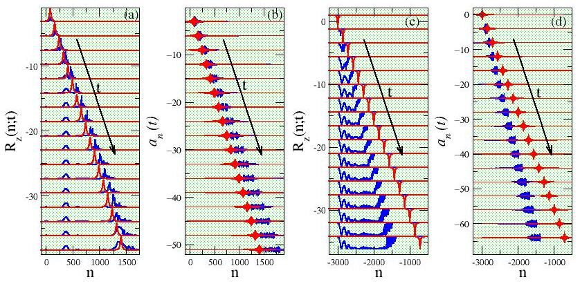
Figure 3: Numerical validation of the analytical expressions for two-photon self-induced transparent (TPSIT) and superradiant (TPSRD) propagating pulses. (a) Snapshots of the population inversion pulse $R_{z}(n;t)$, excited by the induced quantum coherence in the qubit subsystem by the electromagnetic vector potential pulse, in the absence of decoherence ($\gamma=0$); the pulse propagates to the right (time increases downwards) in TPSIT (absorbing) superconducting quantum metamaterials (SCQMMs). The snapshots are taken at intervals of $20$ time-units starting at $t=20$ and they are displaced vertically to avoid overlapping (blue pulses). The corresponding pulses from the analytical expression equation (11) at the same time-instants are shown in red. (b) Snapshots for the corresponding evolution of the electromagnetic vector potential pulse $a_{n}(t)$, that exhibits significant broadening as time passes by; the numerical and analytical pulses are shown in blue and red color, respectively. (c) The same as in a in TPSRD (amplifying) superconducting quantum metamaterials. The resulting propagation is not as simple as expected from the theoretical analysis; instead of a population inversion pulse, it is observed a rather kink-like front propagating to the the right (blue) with a velocity considerably less than that predicted analytically for the pulse, which analytical form is shown in red. (d) The same as in b in TPSRD (amplifying) superconducting quantum metamaterials. The velocity of the $a_{n}(t)$ pulse (blue) is the same as that of the propagating population inversion front, $R_{z}(n;t)$; however, it exhibits less broadening with time in comparison with the corresponding numerical $a_{n}(t)$ pulse in b. The predicted analytical form is shown in red. Parameter values: $\chi=1/5$, $\beta=6$, $V_{00}=V_{11}=1$, $V_{01}=V_{10}=0.8$, $E_{1}-E_{0}=3$, and $v/c=0.7$ (for a and b); $v/c=1.25$ (for c and d).

Numerical Simulations

In order to confirm numerically the obtained results, the equations (3)-(5) and (6) are integrated in time using a fourth order Runge-Kutta algorithm with constant time-step. For pulse propagation in absorbing SCQMMs, all the qubits are initially set to their ground state while the vector potential pulse assumes its analytical form for the given set of parameters. A very fine time-step and very large qubit arrays are used to diminish the energy and/or probability loss and the effects of the boundaries during propagation, respectively. The subsequent temporal evolution in two-photon SIT SCQMM, as can be seen in Figures 3a and 3b, in which several snapshots of the population inversion $R_{z}(n;t)$ and the vector potential pulses $a_{n}(t)$, respectively, are shown, reveals that the latter are indeed capable of inducing quantum coherent effects in the qubit subsystem in the form of population inversion pulses! In Figure 3a, the amplitude of the $R_{z}(n;t)$ pulse gradually grow to the expected maximum around unity in approximately $60$ time units, and they continue its course almost coherently (although with fluctuating amplitude) for about $160$ more time units, during which they move at the same speed as the vector potential pulse (Figure 3b). However, due to the inherent discreteness in the qubit subsystem and the lack of inter-qubit coupling, the $R_{z}(n;t)$ pulse splits at certain instants leaving behind small ”probability bumps” that get pinned at particular qubits. After the end of the almost coherent propagation regime, the $R_{z}(n;t)$ pulse broadens and slows-down until it stops completely. At the same time, the width of the $a_{n}(t)$ pulse increases in the course of time due to discreteness-induced dispersion. A comparison with the corresponding analytical expressions reveals fair agreement during the almost coherent propagation regime, although both the $R_{z}(n;t)$ and $a_{n}(t)$ pulses travel slightly faster than expected from the analytical predictions. The temporal variable here is normalized to the inverse of the Josephson frequency $\omega_{J}$ which for typical parameter values is of the order of a few $GHz$ Rakhmanov2008 . Then, the almost coherent induced pulse regime in the particular case shown in Figure 3 lasts for $\sim 160\times 10^{-9}$ s, or $\sim 160~{}ns$, which is of the same order as the reported decoherence time for a charge qubit in Gambetta2006 (i.e., $200~{}ns$).

The situation seems to be different, however, in the case of two-photon SRD pulses, as can be observed in the snapshots shown in Figures 3c and 3d for $R_{z}(n;t)$ and $a_{n}(t)$, respectively. Here, the lack of the inter-qubit interaction is crucial, since the SCQs that make a transition from the excited to their ground state as the peak of the $a_{n}(t)$ pulse passes by their location, cannot return to their excited states after the $a_{n}(t)$ pulse has gone away. It seems, thus, that the $a_{n}(t)$ pulse creates a type of a kink-like front that propagates at the same velocity. It should be noted that the common velocity of the $R_{z}(n;t)$ and $a_{n}(t)$ pulses is considerably different (i.e., smaller) than the analytically predicted one, as it can be inferred by inspection of Figures 3c and 3d. Even more complicated behavioral patterns of two-photon SRD propagating pulses and the effect of non-zero decoherence factor are discussed in the Supplementary Information.

Conclusion

An SCQMM comprising SCQs loaded periodically on a superconducting TL has been investigated theoretically using a minimalistic one-dimensional model following a semiclassical approach. While the SCQs are regarded as two-level quantum systems, the EM field is treated classically. Through analytical techniques it is demonstrated that the system allows self-induced transparent and superradiant pulse propagation given that a particular constraint is fulfilled. Most importanty, it is demonstrated that the propagating EM pulses may induce quantum coherent population inversion pulses in the SCQMM. Numerical simulation of the semiclassical equations confirms the excitation of population inversion pulses with significant coherence time in absorbing media. The situation is slightly different in amplifying media, in which the numerically obtained, induced population inversion excitations are kink-like propagating structures (although more complex behaviors discussed in the Supplementary Information also appear). Moreover, the limiting pulse velocity in both amplifying and absorbing SCQMMs is lower than the corresponding one in two-photon resonant amplifying and absorbing ordinanary (atomic) media. That limiting velocity in SCQMMs can in principle be engineered through the SCQ parameters.

Author Contributions

Z.I., N.L., and G.P.T. performed the research, analyzed the results and wrote the paper.

Additional information

Competing financial interests: The authors declare no competing financial interests.

SUPPLEMENTARY INFORMATION:

QUBIT LATTICE COHERENCE INDUCED BY ELECTROMAGNETIC PULSES

IN SUPERCONDUCTING METAMATERIALS

I Hamiltonian function and Quantization of the Qubit Subsystem

Consider an infinite number of superconducting charge qubits in a transmission line (TL) that consists of two superconducting plates separated by distance $d$, while the center-to-center distance between qubits, $\ell$, is of the same order of magnitude. The charge qubit is of the form of a mesoscopic superconducting island which is connected to each electrode of the TL with a Josephson junction (JJ). Assume that an electromagnetic (EM) wave corresponding to a vector potential $\vec{A}=A_{z}(x,t)\hat{z}$ propagates along the superconducting TL, in a direction parallel to the superconducting electrodes and perpendicular to the direction of the EM wave propagation. A minimalistic description of that system constists of writing the Hamiltonian of the compound qubit array - EM field system with the geometry shown in Fig. 1 of the paper, as

$$H=\sum_{n}\left\{\dot{\varphi}^{2}_{n}-2\cos\alpha_{n}\cos\varphi_{n}+\dot{\alpha}^{2}_{n}+\beta^{2}(\alpha_{n+1}-\alpha_{n})^{2}\right\},$$ (13)

where $\varphi_{n}$ is the superconducting phase on $n-$th island, $\beta^{2}=(8\pi dE_{J})^{-1}\left(\Phi_{0}/(2\pi)\right)^{2}$, with $d$ being the separation between the superconducting electrodes of the TL, and the overdots denote derivation with respect to the temporal variable $t$. In what follows, a basic assumption is that the wavelength $\lambda$ of the EM field is much larger than the other length scales determined by the size of the unit cell of the qubit metamaterial ($\lambda>>\ell,d$), so that the vector potential component $A_{z}(x,t)$ can be regarded to be approximatelly constant within a unit cell, $A_{z}(x,t)\simeq A_{z,n}(t)$. Then, the discretized and normalized EM vector potential at the $n-$th unit cell which appears in Eq. (13) reads $a_{n}(t)=(2\pi d/\Phi_{0})A_{n}(t)$. The Hamiltonian function Eq. (13) is given in units of the Josephson energy $E_{J}=(\Phi_{0}I_{c})/(2\pi C)$, where $I_{c}$ and $C$ is the critical current and capacitance, respectively, of the JJs, and $\Phi_{0}=h/(2e)$ is the flux quantum, with $h$ and $e$ being the Planck’s constant and the electron charge, respectively. That Hamiltonian can be written in a more transparent form by adding and subtracting $2\cos\phi_{n}$ and subsequently rearranging to get

$$H=H_{QUB}+H_{EMF}+H_{int},$$ (14)

where the qubit subsystem energy $H_{QUB}$, the EM field energy $H_{EMF}$, and their interaction energy $H_{int}$, take respectively the form

$$H_{QUB}=\sum_{n}\{\dot{\varphi}^{2}_{n}-2\cos\varphi_{n}\},\qquad H_{EMF}=\sum_{n}\{\dot{\alpha}^{2}_{n}+\beta^{2}(\alpha_{n+1}-\alpha_{n})^{2}\},\qquad H_{int}=\sum_{n}\{2\cos\varphi_{n}(1-\cos\alpha_{n})\}.$$ (15)

In the following, the EM field is treated classically, while the qubits are regarded as two-level systems. The latter approximation is particularly well suited in the case of resonant qubit - EM field interaction adopted here.

The quantization of the qubit subsystem can be formally performed by replacing the classical variables $\varphi_{n}$ and $\dot{\varphi}_{n}$ by the quantum operators $\hat{\varphi_{n}}$ and $\dot{\varphi}_{n}\rightarrow-i\frac{\partial}{\partial\varphi_{n}}$, respectively, in the Hamiltonian $H_{QUB}$ since we are dealing with a large number of Cooper pairs. The exact energy spectrum $E_{p}(n)$ and the corresponding wavefunctions $\Xi_{p}(n)$ of the $n$th qubit may then be obtained by mapping the Schrödinger equation with the single-qubit Hamiltonian $H_{sq}=\dot{\varphi}_{n}^{2}-2\cos\varphi_{n}$, onto the Mathieu equation

$$\bigg{(}\frac{\partial^{2}}{\partial\varphi^{2}_{n}}+E_{p,n}-2\cos\varphi_{n}\bigg{)}\Xi_{p,n}=0.$$ (16)

The second quantization of the qubit subsystem proceeds by rewritting the single-qubit Hamiltonian as

$$H_{sq}\rightarrow H_{sq}=-\int d\varphi_{n}\hat{\Psi}^{\dagger}(\varphi)\bigg{(}\frac{\partial^{2}}{\partial\varphi^{2}}+2\cos\varphi\bigg{)}\hat{\Psi}(\varphi),$$ (17)

where $\hat{\Psi}^{\dagger}$ and $\hat{\Psi}$ are field operators. Note that the subscript $"n"$ in Eq. (17) has been dropped since the qubits are identical. Using the expansion $\hat{\Psi}(\varphi)=\sum_{p}a_{p}\Xi_{p}(\varphi)$, where the operators $a^{\dagger}_{p}$ ($a_{p}$) create (annihilate) qubit excitations of energy $E_{p}$, the Hamiltonian Eq. (17) is transformed into

$$H_{sq}=\sum_{p=0,1,...}E_{p}a^{\dagger}_{p}a_{p}.$$ (18)

We hereafter restrict $H_{sq}$ to the Hilbert subspace of its two lowest levels, i.e., those with $p=0,1$, so that in second quantized form the Hamiltonian Eq. (14) reads

$$H=\sum_{n}\sum_{p}E_{p}(n)a^{\dagger}_{n,p}a_{n,p}+\sum_{p,p^{\prime}}V_{p,p^{\prime}}(n)a^{\dagger}_{n,p}a_{n,p^{\prime}}\sin^{2}\frac{\alpha_{n}}{2}+\sum_{n}\{\dot{\alpha}^{2}_{n}+\beta^{2}(\alpha_{n+1}-\alpha_{n})^{2}\},$$ (19)

where $p,p^{\prime}=0,1$ and the $V_{p,p^{\prime}}(n)\equiv V_{p^{\prime},p}(n)$ that represent the matrix elements of the $n$th qubit - EM field interaction, are given by

$$V_{p,p^{\prime}}(n)=\int d\varphi_{n}\Xi^{*}_{p}(\varphi_{n})\cos\varphi_{n}\Xi_{p,n}(\varphi_{n}).$$ (20)

In the reduced state space, in which a single qubit can be either in the ground ($p=0$) or in the excited ($p=1$) state, the normalization condition $\sum_{p}a^{\dagger}_{n,p}a_{n,p}=1$ holds for each qubit in the metamaterial. The reduced Hamiltonian Eq. (19) is also written in units of $E_{J}$.

II Maxwell-Bloch Formulation of the Dynamic Equations

In accordance with the adopted semiclassical approach, the time-dependent Schrödinger equation

$$i\hbar\frac{\partial}{\partial t}|\Psi\rangle=\bar{H}|\Psi\rangle,$$ (21)

in which $\bar{H}$ is the Hamiltonian from Eq. (19) in physical units, i.e., $\bar{H}=HE_{J}$, is employed for the description of the qubit subsystem. Generally, the state of each qubit is a superposition of the form

$$|\Psi_{n}\rangle=\sum_{p}\Psi_{n,p}(t)a^{\dagger}_{n,p}|0\rangle,$$ (22)

for which it can be easily shown that the coefficients $\Psi_{n,p}$ satisfy the following normalization conditions

$$\sum_{p}|\Psi_{n,p}(t)|^{2}=1,\qquad\sum_{n,p}|\Psi_{n,p}(t)|^{2}=N,$$ (23)

where in the second Eqs. (23) a finite $N-$qubit subsystem has been implied. Assuming that the pulse power is not very strong, substantial simplification of the dynamic equations for the qubit subsystem can be achieved using the approximation $[1-\cos(\alpha_{n})]\simeq(1/2)\alpha^{2}_{n}$ in the interaction Hamiltonian $H_{int}$. Substitution of $|\Psi\rangle=|\Psi_{n}\rangle$ from Eq. (22) into the Schrödinger equation (21), along with derivation of the classical Hamilton’s equation for the normalized EM vector potential $\alpha_{n}$, yields

$$i\dot{\Psi}_{n,p}=\epsilon_{p}\Psi_{n,p}+\frac{1}{\chi}\sum_{p^{\prime}}V_{p,p^{\prime}}(n){\Psi}_{n,p^{\prime}}\alpha^{2}_{n},$$ (24)

$$\ddot{\alpha}_{n}-\beta^{2}(\alpha_{n+1}+\alpha_{n-1}-2\alpha_{n})+\sum_{p,p^{\prime}}V_{p,p^{\prime}}\Psi^{*}_{n,p}\Psi_{n,p^{\prime}}\alpha_{n}=0,$$ (25)

where $\chi=\hbar\omega_{j}/E_{J}$. In Eqs. (24) and (25), the temporal variable is renormalized according to $t\rightarrow\omega_{J}t$. Because of that, the dimensionless energy of the qubit excitations has to be redefined according to $E_{P}\rightarrow\epsilon_{p}=E_{p}/\chi$, which explains the presence of the dimensionless factor $1/\chi$ in Eq. (24).

The evolution Eqs. (24) and (25) can be rewritten in terms of the $n-$dependent Bloch vector components through the transformation

$$R_{z}(n)=|\Psi_{n,1}|^{2}-|\Psi_{n,0}|^{2},\qquad R_{y}(n)=i(\Psi^{*}_{n,0}\Psi_{n,1}-\Psi^{*}_{n,1}\Psi_{n,0}),\qquad R_{x}(n)=\Psi^{*}_{n,1}\Psi_{n,0}+\Psi^{*}_{n,0}\Psi_{n,1}.$$ (26)

in which the variables $R_{i}$ ($i=x,y,z$) apply to each single qubit. Thus, from the point of view of a macroscopic system, $|\Psi_{i}|^{2}$ represent the population densities $\varrho_{i}=\frac{N}{N}|\Psi|^{2}\equiv\frac{N_{i}}{N}$. By transforming Eqs. (24) and (25) according to Eq. (26) we get

$$\dot{R}_{x}(n)=-(\Delta+2D\alpha_{n}^{2})R_{y}(n),\qquad\dot{R}_{y}(n)=+(\Delta+2D\alpha_{n}^{2})R_{x}(n)-2\mu\alpha_{n}^{2}R_{z}(n),\qquad\dot{R}_{z}(n)=+2\mu\alpha_{n}^{2}R_{y}(n),$$ (27)

$$\ddot{\alpha}_{n}+\chi[\Omega^{2}+\mu R_{x}(n)+DR_{z}(n)]\alpha_{n}=\beta^{2}(\alpha_{n-1}-2\alpha_{n}+\alpha_{n+1}),$$ (28)

where

$$D=\frac{(V_{11}-V_{00})}{2\chi},\qquad\Omega^{2}=\frac{(V_{11}+V_{00})}{2},\qquad\mu=\frac{V_{10}}{\chi},\qquad\Delta=\epsilon_{1}-\epsilon_{0}\equiv\frac{(E_{1}-E_{0})}{\chi}.$$ (29)

By taking the continuous limit of Eqs. (27) and (28) using the relations $\alpha_{n}\rightarrow\alpha(x,t)$ and $\alpha_{n\pm 1}\approx\alpha\pm\alpha_{x}+\frac{1}{2}\alpha_{xx}$, we obtain

$$\dot{R}_{x}=-(\Delta+2D\alpha^{2})R_{y},\qquad\dot{R}_{y}=+(\Delta+2D\alpha^{2})R_{x}-2\mu\alpha^{2}R_{z},\qquad\dot{R}_{z}=+2\mu\alpha^{2}R_{y},$$ (30)

$$\ddot{\alpha}-\beta^{2}\alpha_{xx}+\Omega^{2}\alpha=-\chi(DR_{z}+\mu R_{x})\alpha,$$ (31)

where $R_{x}$, $R_{y}$, $R_{z}$, and $\alpha$ are functions of the spatial variable $x$ and normalized temporal variable $t$, while the overdots denote partial derivation with respect to the latter. It can be easily verified that the Bloch equations Eqs. (30) possess the dynamic invariant $\sum_{i}R^{2}_{i}=1$, whose constant value is derived through the normalization conditions.

III Slowly Varying Envelope Approximation (SVEA)

The Slowly Varying Envelope Approximation (SVEA) relies on the assumption that the envelop of a travelling pulse in a nonlinear medium varies slowly in both time and space compared with the period of the carrier wave, that makes possible the introduction of slow and fast variables. Assuming that in the following, we can approximate the EM vector potential function by

$$\alpha(x,t)=\varepsilon(x,t)\cos\psi(x,t),$$ (32)

where $\psi(x,t)=kx-\omega t+\phi(x,t)$, with $k$ and $\omega$ being the wavenumber and frequency of the carrier wave, respectively, that are connected through the dispersion relation that is obtained at a later stage. The functions $\varepsilon(x,t)$ and $\phi(x,t)$ in Eq. (32) are the slowly varying envelop and phase, respectively. Using fast and slow variables, the $x$ and $y$ Bloch vector components, $R_{x}(n)$ and $R_{y}(n)$, can be expressed as a function of new, in-phase and out-of-phase Bloch vector components $r_{x}$ and $r_{y}$ as

$$R_{x}=r_{x}\cos(2\psi)+r_{y}\sin(2\psi),\qquad R_{y}=r_{y}\cos(2\psi)-r_{x}\sin(2\psi),\qquad R_{z}=r_{z}.$$ (33)

III.1 Derivation of the dynamic equations for the slowly varying envelop and phase of the electromagnetic vector potential

From Eqs. (32) and (33), the second temporal and spatial derivative of $\alpha(x,t)$ can be approximated by

$$\ddot{\alpha}\approx 2\omega\dot{\varepsilon}\sin\psi+(2\omega\dot{\phi}-\omega^{2})\varepsilon\cos\psi,\qquad\alpha_{xx}\approx-2k\varepsilon_{x}\sin\psi-(2k\phi_{x}-k^{2})\varepsilon\cos\psi,$$ (34)

in which the rapidly varying terms of the form $\ddot{\varepsilon}$, $\varepsilon_{xx}$, $\phi^{2}$, $\phi_{xx}$, $\ddot{\phi}$, $\phi_{x}\varepsilon_{x}$, etc., have been neglected. Substitution of Eqs. (34) and (33), into Eq. (31) gives

$$2(\omega\dot{\varepsilon}+k\beta^{2}\varepsilon_{x})\sin\psi+[2(\dot{\phi}\omega+k\phi_{x})-\omega^{2}+\Omega^{2}+\beta^{2}k^{2}]\varepsilon\cos\psi=-\chi\{Dr_{z}+\mu[r_{x}\cos(2\psi)+r_{y}\sin(2\psi)]\}\varepsilon\cos\psi.$$ (35)

Equating the coefficients of $\sin\psi$ and $\cos\psi$ in the earlier equation yields

$$\omega\dot{\varepsilon}+k\beta^{2}\varepsilon_{x}=-\chi\mu r_{y}\varepsilon\cos^{2}\psi,$$ (36)

and

$$2(\dot{\phi}\omega+k\phi_{x})-\{\omega^{2}-\Omega^{2}-\beta^{2}k^{2}\}=-\chi[Dr_{z}+\mu r_{x}\cos(2\psi)].$$ (37)

In order to obtain the dispersion relation $\omega=\omega(k)$, we require the vanishing of the expression in the curly brackets in Eq. (37), which yields for the wavevector of the EM radiation (i.e., the pulse) in the TL the expression

$$k=\pm\frac{\sqrt{\omega^{2}-\Omega^{2}}}{\beta}.$$ (38)

Thus, the EM wave can propagate through the superconducting quantum metamaterial only when its frequency exceeds a critical one, $\omega_{c}=\Omega=\sqrt{(V_{00}+V_{11})/2}$. Finally, Eqs. (36) and (37) are averaged in time over the period $T=2\pi/\omega$ (i.e., the fast time-scale) of the phase $\psi(x,t)$. Due to the simple time-dependence of $\psi(x,t)$ that has been assumed earlier in the framework of SVEA, that averaging actually requires the calculation of integrals of the form

$$\langle{\cal F}(\sin f(\psi),\cos g(\psi))\rangle=\frac{1}{2\pi}\int^{2\pi}_{0}{\cal F}(\sin f(\psi),\cos g(\psi))d\psi.$$

This procedure, when it is applied to the two evolution equations Eqs. (36) and (37) gives the truncated equations for slow amplitude and phase

$$\dot{\varepsilon}+c\varepsilon_{x}=-\chi\frac{\mu}{2\omega}\varepsilon r_{y},\qquad\dot{\phi}+c\phi_{x}=-\chi\frac{D}{\omega}R_{z},$$ (39)

where $c=\beta^{2}k/\omega$ is a critical velocity.

III.2 Derivation of dynamic equations for the transformed Bloch vector components

Substituting Eqs. (32) and (33) into Eqs. (30) for the original Bloch vector components, we get

$$(\dot{r}_{x}+2\dot{\psi}r_{y})\cos(2\psi)+(\dot{r}_{y}-2\dot{\psi}r_{x})\sin(2\psi)=-(\Delta+2D\varepsilon^{2}\cos^{2}\psi)[r_{y}\cos(2\psi)-r_{x}\sin(2\psi)]$$ (40)

$$(\dot{r}_{y}-2\dot{\psi}r_{x})\cos(2\psi)-(\dot{r}_{x}+2\dot{\psi}r_{y})\sin(2\psi)=(\Delta+2D\varepsilon^{2}\cos^{2}\psi)[r_{x}\cos(2\psi)+r_{y}\sin(2\psi)]-2\mu\varepsilon^{2}\cos^{2}\psi r_{z}$$ (41)

$$\dot{r}_{z}=2\mu\varepsilon^{2}\cos^{2}\psi[r_{y}\cos(2\psi)-r_{x}\sin(2\psi)].$$ (42)

In order to derive the dynamic equations for the new Bloch vector components $r_{i}$, we first multiply Eqs. (40) and (41) by $\cos(2\psi)$ and $\sin(2\psi)$, respectively, and then subtract one equation from the other. Thus we get

$$\dot{r}_{x}+2\dot{\psi}r_{y}=-(\Delta+2D\varepsilon^{2}\cos^{2}\psi)r_{y}+2\mu\varepsilon^{2}\cos^{2}\psi\cos(2\psi)r_{z}.$$ (43)

Similarly, by multiplying Eqs. (40) and (41) by $\sin(2\psi)$ and $\cos(2\psi)$, respectively, and by adding them, we get

$$\dot{r}_{y}-2\dot{\psi}r_{x}=(\Delta+2D\varepsilon^{2}\cos^{2}\psi)r_{x}-2\mu\varepsilon^{2}\cos^{2}\psi\sin(2\psi)r_{z}.$$ (44)

Finally, an average over the phase $\psi$ is performed onto Eqs. (42)-(44) using the (easy to prove) relations $\langle\cos^{2}\psi\cos(2\psi)\rangle=1/4$ and $\langle\cos^{2}\psi\sin(2\psi)\rangle=0$. That procedure, and using also the relation $\dot{\psi}=\dot{\phi}-\omega$, yields the truncated Bloch equations

$$\dot{r}_{x}=-(\delta+2\dot{\phi}+D\varepsilon^{2})r_{y}-\frac{\mu}{2}\varepsilon^{2}r_{z},\qquad\dot{r}_{y}=+(\delta+2\dot{\phi}+D\varepsilon^{2})r_{x},\qquad\dot{r}_{z}=\frac{\mu}{2}\varepsilon^{2}r_{y},$$ (45)

where $\delta=\Delta-2\omega$. Note that Eqs. (45) possess a dynamic invariant that has a form similar to that of the original Bloch equations, Eqs. (30), i.e.,

$$r^{2}_{x}+r^{2}_{y}+r^{2}_{z}=1.$$ (46)

The truncated Bloch equations Eqs. (45), along with Eqs. (39) for the slowly varying amplitude and phase of the EM vector potential pulse, constitute a closed system with five unknown functions which describe the approximate dynamics of the superconducting quantum metamaterial that are determined in the next section.

IV Exact Integration of the Truncated Equations

The combination of Eqs. (39) and the third equation of Eqs. (45) provides a relation between the slow amplitude and the phase of the EM vector potential pulse. The first of Eqs. (39) is multiplied by $\varepsilon$ and written as

$${\left[\frac{\partial}{\partial t}+c\frac{\partial}{\partial x}\right]\varepsilon^{2}(x,t)}=-\chi\frac{\mu}{\omega}\varepsilon^{2}(x,t)r_{y},$$ (47)

while the derivative of the second of Eqs. (39) is taken with respect to time and then $\dot{R}_{z}=\dot{r}_{z}$ is replaced from Eqs. (45). Thus we get

$${\left[\frac{\partial}{\partial t}+c\frac{\partial}{\partial x}\right]\dot{\phi}(x,t)}=-\chi\frac{\mu D}{2\omega}\varepsilon^{2}(x,t)r_{y}.$$ (48)

From Eqs. (47) and (48), and by taking into account the independence of the slow temporal and spatial variables, we get

$$2\dot{\phi}(x,t)=D\varepsilon^{2}(x,t)+const.,$$ (49)

where the constant of integration can be set equal to zero. Using Eq. (49), the truncated Bloch equations Eqs. (45) can be written as

$$\dot{r}_{x}=-(\delta+2D\varepsilon^{2})r_{y},\qquad\dot{r}_{y}=+(\delta+2D\varepsilon^{2})r_{x}-\frac{\mu}{2}\varepsilon^{2}r_{z},\qquad\dot{r}_{z}=\frac{\mu}{2}\varepsilon^{2}r_{y}.$$ (50)

The latter can be written in a simpler form using the unitary transformation

$$r_{x}=S_{x}\cos\Phi-S_{z}\sin\Phi,\qquad r_{y}=S_{y},\qquad r_{z}=S_{z}\cos\Phi+S_{x}\sin\Phi,$$ (51)

where $\Phi$ is the constant transformation angle that is going to be determined. The truncated Bloch equations for the $r_{i}$, $i=x,y,z$, can be written in terms of the new Bloch vector components $S_{i}$, using a procedure similar to that used in Subsection III.B to obtain Eqs. (45). Sustituting Eqs. (51) into Eqs. (50), we get

$$\dot{S}_{x}\cos\Phi-\dot{S}_{z}\sin\phi=-(\delta+2D\varepsilon^{2})S_{y},$$ (52)

$$\dot{S}_{y}=\left[(\delta+2D\varepsilon^{2})\cos\Phi-\frac{\mu}{2}\varepsilon^{2}\sin\Phi\right]S_{x}-\left[(\delta+2D\varepsilon^{2})\sin\Phi+\frac{\mu}{2}\varepsilon^{2}\cos\Phi\right]S_{z},$$ (53)

$$\dot{S}_{x}\sin\Phi+\dot{S}_{z}\cos\Phi=-\frac{\mu}{2}\varepsilon^{2}S_{y}.$$ (54)

Multiplying Eqs. (52) and (54) by $\cos\Phi$ and $\sin\Phi$, respectively, and then adding them together, we get

$$\dot{S}_{x}=\left\{\varepsilon^{2}\left[\frac{1}{2}\mu\sin\Phi-2D\cos\Phi\right]-\delta\cos\Phi\right\}S_{y}.$$ (55)

Similarly, multiplying Eqs. (52) and (54) by $\sin\Phi$ and $\cos\Phi$, respectively, and then subtracting one equation from the other, we get

$$\dot{S}_{z}=\left\{\varepsilon^{2}\left[\frac{1}{2}\mu\cos\Phi+2D\sin\Phi\right]-\delta\sin\Phi\right\}S_{y}.$$ (56)

The transformation angle $\Phi$ can now be selected so that the resulting equations are simplified as much as possible. We thus define

$$\tan\Phi\equiv\gamma=\frac{4D}{\mu},$$ (57)

so that $\cos\Phi=\pm\sigma$ and $\sin\Phi=\pm\sigma\gamma$ where $\sigma=1/\sqrt{1+\gamma^{2}}$. The choice of the sign is irrelevant and here we pick positive sign for both functions. Using the above value for the transformation angle and the definitions $W=\sqrt{(4D)^{2}+\mu^{2}}$ and $\eta=-\delta\mu/W$, Eqs. (55), (53), and (56) obtain their final form

$$\dot{S}_{x}=+\eta S_{y},\qquad\dot{S}_{y}=-\eta S_{x}+\left[\eta\gamma-\frac{1}{2}W\varepsilon^{2}\right]S_{z},\qquad\dot{S}_{z}=\left[-\eta\gamma+\frac{1}{2}W\varepsilon^{2}\right]S_{y}.$$ (58)

In order to investigate the possibility for ”coherent propagation” of an electromagnetic potential pulse, we consider resonance conditions. In that case, $\eta=0$, and Eqs. (58) become

$$\dot{S}_{x}=0,\qquad\dot{S}_{y}=-\frac{1}{2}W\varepsilon^{2}S_{z},\qquad\dot{S}_{z}=+\frac{1}{2}W\varepsilon^{2}S_{y}.$$ (59)

Combining the second and third Eq. (59) and integrating, we obtain the ”resonant” conservation law $S_{y}^{2}+S_{z}^{2}=const.$. Assuming that all the qubits are in the ground state at $t=-\infty$, we have the initial conditions $r_{x}(t=-\infty)=r_{y}(t=-\infty)=0$ and $r_{z}(t=-\infty)=-1$ which are transformed into $S_{x}(t=-\infty)=-\gamma\sigma$, $S_{y}(t=-\infty)=0$, and $S_{z}(t=-\infty)=-\sigma$ through the transformation Eq. (51). Applying the initial conditions to the resonant conservation law, we get

$$S_{y}^{2}+S_{z}^{2}=\sigma^{2}.$$ (60)

In the following, we seek solution of the form $\varepsilon=\varepsilon(\tau=t-x/v)$ and $S_{i}=S_{i}(\tau=t-x/v)$, with $i=x,y,z$. By changing the variables in the first of Eqs. (39), with $r_{y}$ being replaced by $S_{y}$, we get after rearramgement

$$\frac{\varepsilon_{\tau}}{\varepsilon}=\chi\frac{\mu}{2\omega}\frac{v}{c-v}S_{y}.$$ (61)

Then, combining Eq. (41) with the third Eq. (59) and integrating, we get

$$\varepsilon^{2}(\tau)=\chi\frac{2\mu}{\omega W}\frac{v}{c-v}[S_{z}(\tau)+\sigma],$$ (62)

where the conditions $\varepsilon(-\infty)$ and $S_{z}(-\infty)=-\sigma$ were used. The system of Eqs. (60)-(62) for $\varepsilon$, $S_{y}$, and $S_{z}$ can be integrated exactly; the variables $S_{y}$ and $S_{z}$ can be eliminated in favour of $\varepsilon$ to give $\varepsilon_{\tau}=\lambda\varepsilon^{2}\sqrt{a+b\varepsilon^{2}}$, in which the constants are defined as $a=2\sigma/\kappa$, $b=-1/\kappa^{2}$, $\lambda=\chi\frac{\mu}{2\omega}\frac{v}{c-v}$, $\kappa=\frac{2\mu}{\omega W}\frac{v}{c-v}$ to simplify the notation. The equation for $\varepsilon$ can be readily integrated

$$\int_{\varepsilon_{0}}^{\varepsilon}\frac{d\varepsilon}{\varepsilon^{2}\sqrt{a+b\varepsilon^{2}}}=\lambda\int_{\tau_{0}}^{\tau}d\tau\Rightarrow-\frac{\sqrt{a+b\varepsilon^{2}}}{a\varepsilon}=\lambda(\tau-\tau_{0}),$$ (63)

where we have set $\varepsilon_{0}\equiv\varepsilon(\tau=\tau_{0})=\sqrt{2\sigma\kappa}$ to eliminate the boundary term resulting from the integral over $\varepsilon$. Solving Eq. (63) for $\varepsilon$, we finally get a Lorentzian-like slowly varying amplitude

$$\varepsilon(\tau)=\frac{\varepsilon_{0}}{\sqrt{1+\tau_{p}^{-2}(\tau-\tau_{0})^{2}}},$$ (64)

where $\varepsilon_{0}=\sqrt{-{a}/{b}}=\sqrt{2\sigma\kappa}$ and $\tau_{p}^{-2}=-\frac{a^{2}\lambda^{2}}{b}=\left(\chi\frac{\sigma\mu}{\omega}\right)^{2}\left(\frac{v}{c-v}\right)^{2}$.

V Details of the Numerical Simulations and the Role of Decoherence

The numerical simulations in order to confirm (or not) the existence of the quantum coherent effects and the quantum coherence induced in the medium, i.e., the qubit transmission line, which are predicted through analytical considerations, consist of integrating Eqs. 3a-3c and 4 of the paper ($n=1,N$)

$$\dot{R}_{x}(n) =-\left[\Delta+8D\sin^{2}\frac{\alpha_{n}}{2}\right]R_{y}(n),$$ (65a)

$$\dot{R}_{y}(n) =\left[\Delta+8D\sin^{2}\frac{\alpha_{n}}{2}\right]R_{x}(n)-8\mu\sin^{2}\frac{\alpha_{n}}{2}R_{z}(n),$$ (65b)

$$\dot{R}_{z}(n) =+8\mu\sin^{2}\frac{\alpha_{n}}{2}R_{y}(n),$$ (65c)

and

$$\ddot{\alpha}_{n}+\chi\left[\Omega^{2}+\mu R_{x}(n)+DR_{z}(n)\right]\sin\alpha_{n}=\beta^{2}\delta a_{n},$$ (66)

where $\delta\alpha_{n}=\alpha_{n-1}-2\alpha_{n}+\alpha_{n+1}$ and the parameters $D$, $\Omega$, $\epsilon_{p}$, $\mu$, $\Delta$, and $\chi$ are defined in the paper as functions of the interaction matrix elements $V_{ij}$ ($i,j=1,2$), the energy difference between the ground and the first excited level, $E_{1}-E_{0}$, and the discrete vector potential coupling parameter $\beta$. The earlier system of ordinary differential equations is integrated in time with a standard fourth order Runge-Kutta algorithm with constant time-step $\Delta t$, typically $10^{-3}$. Such small time-steps, and even smaller sometimes, are required to conserve up to high accuracy the total and partial probabilities as the compound system of qubits and the electromagnetic vector potential evolve in time. In all the simulations, periodic boundary conditions are used. Due to the particular shape (Lorentzian) of the EM vector potential pulse and the population inversion pulse in the qubit subsystem, very large systems with $N=2^{13}=8192$ and $N=2^{14}=16384$ have been simulated to diminish as much as possible the effects from the ends (i.e., the interaction of the pulse tail with itself, as it could be in the case of periodic boundary conditions). In some cases, it is necessary to simulate even larger systems, with $N=50,000$. In the figures presented in the paper and here only part of these arrays is shown, for clarity. In order to observe two-photon self-induced transparent (TPSIT) pulses $a_{n}(t)$ and the induced quantum coherent population inversion pulses $R_{z}(n;t)$, the following initial coditions are implemented: for the former, the analytically obtained solution resulting for the given set of parameters, while for the latter all the qubits are set to their ground, $E_{0}$, state. In terms of the Bloch vector variables $R_{i}$, $i=x,y,z$, that initial condition is specified as:

$$R_{x,y}(t=0)=0,\qquad R_{z}(t=0)=-1,$$ (67)

for any $n=1,...,N$. In that case, the above mentioned pulses exist for velocities less than the corresponding limiting velocity for TPSIT media, i.e.,

$$v<c=\beta^{2}\frac{k}{\omega}=2\beta^{2}\frac{k}{\Delta}.$$ (68)

The last equality is valid only when the two-photon resonance condition $\omega=\Delta/2$ is satisfied. In Eq. (20), $k$ and $\omega$ denote the wavenumber and frequency of the carrier wave of the electromagnetic vector potential; while the latter is determined by the two-photon resonance condition, the former may vary within an interval which is restricted by the qubit-parameter-dependent condition

$$2\chi^{2}(V_{11}+V_{00})<(E_{1}-E_{0})^{2},$$ (69)

that guarantees the wavenumber $k$ being real.

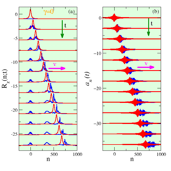
Figure 4: Numerical validation of the analytical expressions for two-photon self-induced transparent (TPSIT) propagating pulses in superconducting quantum metamaterials (SCQMMs) without decoherence. a, Snapshots of the population inversion pulse $R_{z}(n;t)$, excited by the induced quantum coherence in the qubit subsystem by the electromagnetic vector potential pulse, in the absence of decoherence ($\gamma=0$); the pulse propagates to the right (time increases downwards). b, Snapshots for the corresponding evolution of the electromagnetic vector potential pulse $a_{n}(t)$, that exhibits significant broadening while its amplitude decreases as time passes by; the numerical and analytical pulses are shown in blue and red color, respectively. Parameter values: $\chi=1/4.9$, $\beta=6$, $V_{00}=V_{11}=1$ ($\gamma=0$), $V_{01}=V_{10}=0.7$, $E_{1}-E_{0}=3$, and $v/c=0.7$.

The role of decoherence in TPSIT in superconducting quantum metamaterials like the one investigated here can be observed in Figures 4, 5, and 6, in which the amount of decoherence, quantified by the factor $\gamma$, takes the values $0$, $0.01$ and $0.1$, respectively. The decoherence factor $\gamma$ depends solely on the interaction matrix elements $V_{ij}$; it is given by

$$\gamma=2\frac{V_{11}-V_{00}}{V_{10}},$$ (70)

i.e., it is equal to zero for $V_{00}=V_{11}$ while it assumes non-zero values for $V_{11}>V_{00}$. The Figures 4-6 show snapshots of $R_{z}(n;t)$ and $a_{n}(t)$ at several instants from $t=0$ to $t=168$, which are separated by $14$ time units, along with the corresponding analytical solutions. All these profiles but the first are shifted downwards to avoid overlapping, while only part of the array is shown for clarity. Note that time increases downwards. In Figure 4, for $\gamma=0$, the $a_{n}(t)$ pulse is observed to excite a population inversion pulse $R_{z}(n;t)$ in the qubit subsystem (Figure 4a). The amplitude of $R_{z}(n;t)$ gradually increases until it attains its maximum value close to unity, while at the same time it propagates to the right with velocity $v^{\prime}$. In the figure, that occurs for the first time at $t\simeq 70$ time units; subsequently it evolves in time while it keeps its amplitude almost constant for at least $56$ time units. After that, its amplitude starts decreasing until it is completely smeared (not shown). During the time interval in which the amplitude of the $R_{z}(n;t)$ pulse is close to the predicted one (i.e., close to unity), the metamaterial is considered to be in the almost quantum coherent regime. Note that at about $t=84$ a little bump starts to appear which grows to a little larger (”probability bump”) which gets pinned at a particular site at $n\sim 300$. Note that another such bump appears at $n=0$ due to the initial ”shock” of the qubit subsystem because of the sudden onset of the $a_{n}(t)$ pulse. A comparison of the numerical $R_{z}(n;t)$ profiles with the analytical ones reveals that the velocity of propagation $v^{\prime}$, which is the same as that of the numerical $a_{n}(t)$ pulse (Figure 4b), is slightly larger than the predicted one $v$ ($v^{\prime}>v$). The corresponding profiles for very weak decoherence, in which the value of the decoherence factor $\gamma=0.01$, are shown in Figure 2. For that weak decoherence, there are only slight differences in comparison with Figure 1 which actually cannot be observed in the scale of the figures.

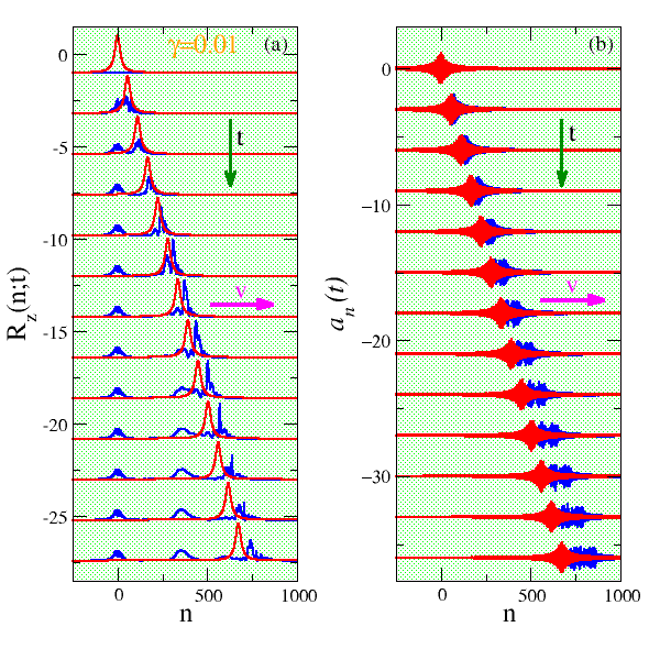
Figure 5: Numerical validation of the analytical expressions for two-photon self-induced transparent (TPSIT) propagating pulses in superconducting quantum metamaterials (SCQMMs) in the presence of weak decoherence. a, Snapshots of the population inversion pulse $R_{z}(n;t)$, excited by the induced quantum coherence in the qubit subsystem by the electromagnetic vector potential pulse, in the absence of decoherence ($\gamma=0.01$); the pulse propagates to the right (time increases downwards). b, Snapshots for the corresponding evolution of the electromagnetic vector potential pulse $a_{n}(t)$, that exhibits significant broadening while its amplitude decreases as time passes by; the numerical and analytical pulses are shown in blue and red color, respectively. Parameter values: $\chi=1/4.9$, $\beta=6$, $V_{00}=0.998$, $V_{11}=1.002$, $V_{01}=V_{10}=0.7$, $E_{1}-E_{0}=3$, and $v/c=0.7$.

In Figure 6, the decoherence factor has acquired a substantial value of $\gamma=0.1$, so that its effects are now clearly observed in the population inversion pulse $R_{z}(n;t)$, while the vector potential pulse $a_{n}(t)$ does not seem to be affected. In Figure 6a, while the $R_{z}(n;t)$ is still excited by the vector potential pulse $a_{n}(t)$, it has a very low amplitude compared with that of the analytically predicted form. Indeed, that amount of decoherence only slightly changes the analytical $R_{z}(n;t)$ pulse and that change is hardly visible in the scale of the figure. Note that the speed of the $R_{z}(n;t)$ is the same as in the case without decoherence (which is also the same with that of the $a_{n}(t)$ pulse, in Figures 4-6); even the unwanted ”probability bumps” appear at about the same locations with almost the same amplitude and shape independently of the amount of decoherence.

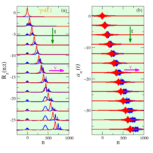
Figure 6: Numerical validation of the analytical expressions for two-photon self-induced transparent (TPSIT) propagating pulses in superconducting quantum metamaterials (SCQMMs) in the presence of substantial decoherence. a, Snapshots of the population inversion pulse $R_{z}(n;t)$, excited by the induced quantum coherence in the qubit subsystem by the electromagnetic vector potential pulse, in the absence of decoherence ($\gamma=0.1$); the pulse propagates to the right (time increases downwards). b, Snapshots for the corresponding evolution of the electromagnetic vector potential pulse $a_{n}(t)$, that exhibits significant broadening while its amplitude decreases as time passes by; the numerical and analytical pulses are shown in blue and red color, respectively. Parameter values: $\chi=1/4.9$, $\beta=6$, $V_{00}=0.98$, $V_{11}=1.02$, $V_{01}=V_{10}=0.7$, $E_{1}-E_{0}=3$, and $v/c=0.7$.

Next, the possibility for the existence of propagating two-photon superradiant pulses in SCQMMs for large values of $\beta$ is numerically explored (Figure 4). In order to obtain that figure, the qubit subsystem is initialized with all the qubits in their excited state, while the vector potential pulse assumes its analytically predicted form for the selected parameter set. A very large array with $N=50,000$ is simulated, and the initial position of the (center of) $a_{n}(t)$ pulse is at $n=-18,750$. The subsequent evolution produces the snapshots presented in Figure 4, from $t=0$ up to $t=300$ time units (time increases downwards). These snapshots are separated in time by $20$ time units and they are displaced vertically to avoid overlapping. The population inversion $R_{z}(n;t)$ and the electromagnetic vector potential pulse $a_{n}(t)$ are shown in Figures 7a and 7b, respectively. In that simulation, the parameter $\beta$ is much larger than that used in Figure 3b of the paper, i.e., here $\beta=30$. The other parameters, except the pulse speed, here $v=2.5>c$, are the same as those used in Figure 3b of the paper.

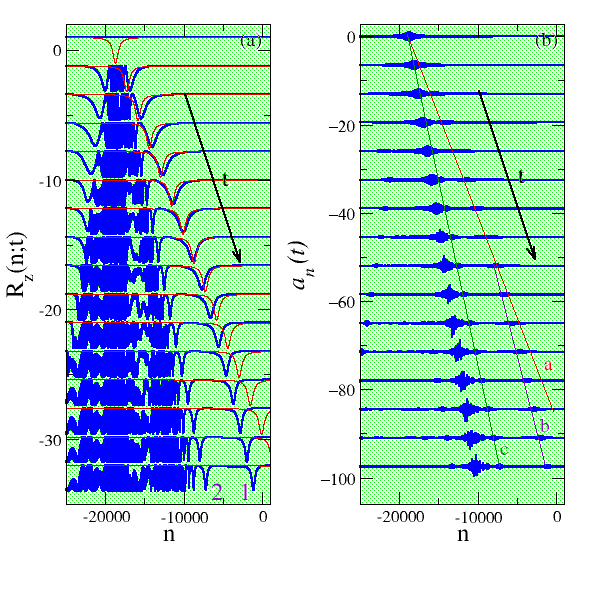
Figure 7: Numerical exploration of the propagation of two-photon superradiant (TPSRD) pulses in superconducting quantum metamaterials (SCQMMs) for large values of $\beta$. a, Snapshots of the population inversion $R_{z}(n;t)$ induced in the qubit subsystem by the electromagnetic vector potential pulse, $a_{n}(t)$ (blue), in the absence of decoherence ($\gamma=0$). The analytically predicted forms are shown in red color. b, Snapshots for the corresponding vector potential pulse $a_{n}(t)$ at the same time-instants. Parameter values: $\chi=1/5$, $\beta=30$, $V_{00}=V_{11}=1$, $V_{01}=V_{10}=0.8$, $E_{1}-E_{0}=3$, and $v/c=2.5$

The spatio-temporal evolution of both pulses reveals a rather complex pattern, that is discussed below. In Figure 4b, the $a_{n}(t)$ pulse breaks into several pulses of different amplitudes and velocities; the most important are discernible along the green (c) and the purple (b) solid lines. In the same subfigure, the red (a) solid line indicates the analytically predicted pulse speed for two-photon superradiance in superconducting quantum metamaterials. The $a_{n}(t)$ pulses emerging from the initial one affect the qubit subsystem in a peculiar and complex way: First of all, a very well-defined $R_{z}(n;t)$ pulse is observed which follows the analytical solution (in red) for quite some time (about $\sim 140$ time units). After that time the pulse (whose last snapshot is numbered $1$) slows down while it gets narrower while it is propagating together with the $a_{n}(t)$ pulse along the purple (b) line. Note that around the initial position of the $a_{n}(t)$ pulse, the population inversion $R_{z}(n;t)$ exhibits a region of strong variability within its extreme values $\pm 1$ which expands in the course of time. At $t\sim 100$ a second $R_{z}(n;t)$ pulse is observed to emerge from the strong variability region, which is significantly narrower than the analytical solution. That second pulse ((whose last snapshot is numbered $2$) propagates slower than the first one ($1$), along with the $a_{n}(t)$ pulse which can be observed along the green line (c) of Figure 7b.

References

- (1) Devoret, M. H. Schoelkopf, R. J. Superconducting circuits for quantum information: An outlook. Science 339, 1169–1174 (2013).
- (2) Georgescu, I. M., Ashhab, S. Nori, F. Quantum simulation. Rev. Mod. Phys. 86, 153–185 (2014).
- (3) Paraoanu, G. S. Recent progress in quantum simulation using superconducting circuits. J. Low Temp. Phys. 175, 633–654 (2014).
- (4) Blatt, R. Roos, C. F. Quantum simulations with trapped ions. Nature Phys. 8, 277–284 (2012).
- (5) Bloch, I., Dalibard, J. Nascimbéne, S. Quantum simulations with ultracold quantum gases. Nature Phys. 8, 267–276 (2012).
- (6) Aspuru-Guzik, A. Walther, P. Photonic quantum simulators. Nature Phys. 8, 285–291 (2012).
- (7) Press, D., Ladd, T. D., Zhang, B. Y. Yamamoto, Y. Complete quantum control of a single quantum dot spin using ultrafast optical pulses. Nature 456, 218–221 (2008).
- (8) Houck, A. A., Türeci, H. E. Koch, J. On-chip quantum simulation with superconducting circuits. Nature Phys. 8, 292–299 (2012).
- (9) Schmidt, S. Koch, J. Circuit QED lattices. Ann. Phys. (Berlin) 525, 395–412 (2013).
- (10) Josephson, B. D. Possible new effects in superconductive tunnelling. Phys. Lett. A 1, 251–255 (1962).
- (11) Wendin, G. Shumeiko, V. S. Quantum bits with Josephson junctions. Low Temp. Phys. 33, 724–744 (2007).
- (12) Pashkin, Yu. A., Astavief, O., Yamamoto, T., Nakamura, Y. Tsai, J. S. Josephson charge qubits: a brief review. Quantum Inf. Process 8, 55–80 (2009).
- (13) Astavief, O. et al. Single artificial-atom lasing. Nature 449, 588–590 (2007).
- (14) Jung, P., Ustinov, A. V. Anlage, S. M. Progress in superconducting metamaterials. Supercond. Sci. Technol. 27, 073001 (2014).
- (15) Macha, P. et al. Implementation of a quantum metamaterial using superconducting qubits. Nat. Commun. 5, art. no. 5146 (2014).
- (16) Asai, H., Savel’ev, S., Kawabata, S. Zagoskin, A. M. Effects of lasing in a one-dimensional quantum metamaterial. Phys. Rev. B 91, 134513 (2015).
- (17) Rakhmanov, A. L., Zagoskin, A. M., Savel’ev, S. Nori, F. Quantum metamaterials: Electromagnetic waves in a Josephson qubit line. Phys. Rev. B 77, 144507 (2008).
- (18) Shvetsov, A., Satanin, A. M., Nori, F., Savel’ev, S. Zagoskin, A. M. Quantum metamaterial without local control. Phys. Rev. B 87, 235410 (2013).
- (19) Zagoskin, A. M. Quantum Engineering: Theory and Design of Quantum Coherent Structures, Cambridge University Press, Cambridge, 2011, (p. 280).
- (20) van Loo, A. F. et al. Photon-mediated interactions between distant artificial atoms. Science 342, 1494–1496 (2013).
- (21) McCall, S. L. Hahn, E. L. Self-induced transparency by pulsed coherent light. Phys. Rev. Lett. 18, 908–911 (1967).
- (22) Dicke, R. H. Coherence in spontaneous radiation processes. Phys. Rev. 93, 99–110 (1954).
- (23) Scheibner, M. et al. Superradiance of quantum dots. Nature Phys. 3, 106–110 (2007).
- (24) Hamner, C. et al. Dicke-type phase transition in a spin-orbit coupled Bose-Einstein condensate. Nat. Comms. 5, 4023 (2014).
- (25) Cornell, E. A. Stopping light in its tracks. Nature 409, 461–462 (2001).
- (26) Gambetta, J. et al. Qubit-photon interactions in a cavity: Measurement-induced dephasing and number splitting. Phys. Rev. A 74, 042318 (2006).
- (27) Belenov, E. M. Poluektov, I. A. Coherence effects in the propagation of an ultrashort light pulse in a medium with two-photon resonance absorption. Sov. Phys. JETP 29, 754–756 (1969).
- (28) Tan-no, N., Yokoto, K. Inaba, H. Two-photon self-induced transparency in a resonant medium I. Analytical treatment. J. Phys. B 8, 339–348 (1975).
- (29) Nayfeh, M. H.. Self-induced transparency in two-photon transition. Phys. Rev. A 18, 2550–2556 (1978).
- (30) John, S. Rupasov, V. I. Quantum self-induced transparency in frequency gap media. Europhys. Lett. 46, 326–331 (1999).
- (31) Park, Q.-H. Boyd, R. W. Modification of self-induced transparency by a coherent control field. Phys. Rev. Lett. 86, 2774–2777 (2001).
Acknowledgements
This work was partially supported by the European Union Seventh Framework Programme (FP7-REGPOT-2012-2013-1) under grant agreement no 316165, the Serbian Ministry of Education and Science under Grants No. III–45010, No. OI–171009, the Ministry of Education and Science of the Republic of Kazakhstan (Contract No. 339/76-2015), and the Ministry of Education and Science of the Russian Federation in the framework of the Increase Competitiveness Program of NUST ”MISiS”(No. K2-2015-007).