Stochastic gravitational wave background from magnetic deformation of newly born magnetars

Abstract

Newly born magnetars are promising sources for gravitational wave (GW) detection due to their ultra-strong magnetic fields and high spin frequencies. Within the scenario of a growing tilt angle between the star’s spin and magnetic axis, due to the effect of internal viscosity, we obtain improved estimates of the stochastic gravitational wave backgrounds (SGWBs) from magnetic deformation of newly born magnetars. We find that the GW background spectra contributed by the magnetars with ultra-strong toroidal magnetic fields of $10^{17}$ G could roughly be divided into four segments. Most notably, in contrast to the background spectra calculated by assuming constant tilt angles $\chi=\pi/2$, the background radiation above 1000 Hz are seriously suppressed. However, the background radiation at the frequency band $\sim 100-1000$ Hz are moderately enhanced, depending on the strengths of the dipole magnetic fields. We suggest that if all newly born magnetars indeed have toroidal magnetic fields of $10^{17}$ G, the produced SGWBs should show sharp variations with the observed frequency at several tens to about 100 hertz. If these features could be observed through sophisticated detection of the SGWB using the proposed Einstein Telescope, it will provide us a direct evidence of the tilt angle evolutions and further some deep understandings about the properties of newly born magnetars.

1 INTRODUCTION

Neutron stars (NSs) are one of the most promising targets for gravitational wave (GW) detection with the ground based GW interferometers such as LIGO, Virgo, GEO600, advanced LIGO (aLIGO) and the proposed Einstein Telescope (ET; see Sathyaprakash & Schutz 2009 for a review). In general, GWs can be radiated from NSs because of many different reasons, e.g., magnetic deformation of the NSs (Bonazzola & Gourgoulhon 1996; Regimbau & de Freitas Pacheco 2001, 2006a; Stella et al. 2005; Dall’Osso et al. 2009; Marassi et al. 2011), dynamical bar-mode instability (Lai & Shapiro 1995), r-mode instabilities due to GW radiation back-reaction (Andersson 1998; Friedman & Morsink 1998; Zhu et al. 2011), oscillations or flows excited by glitches (Abadie et al. 2011; Stopnitzky & Profumo 2014), collapse induced by phase transition to quark matter (Marranghello et al. 2002; Sigl 2006), and coalescences of compact binaries (i.e., NS–NS, NS–white dwarf, or NS–black hole; Schneider et al. 2001; Regimbau & de Freitas Pacheco 2006b; Regimbau & Chauvineau 2007; Zhu et al. 2013). For a newly born NS of interest here, which if spins initially at the mass-shedding limit with a millisecond period and has an ultra-strong magnetic field, it could generate a prompt GW signal due to the bar- and r-mode instabilities and a continuous GW radiation due to a magnetically-induced quadrupole ellipticity. Such an ellipticity is mainly determined by the equation of state (EOS) of the NS, the magnetic configuration in the stellar interior and, most importantly, the magnetic energy (Haskell et al. 2008; Dall’Osso et al. 2009).

It is difficult, usually impossible, to detect GW radiation from magnetic deformation of the Galactic NSs. For canonical NSs such as the Crab pulsar and the central compact object harbouring in Cassiopeia A, their present magnetic fields are obviously too low to sustain a sufficiently high ellipticity. Direct searches for GWs from nearby pulsars has put an upper limit of $\epsilon\lesssim 7\times 10^{-8}$ at 95% confidence level for the pulsars (Abbott et al. 2010). Meanwhile, for the Galactic magnetars whose magnetic fields could be high enough, their long spin periods ($P\sim 2-12$ s; Olausen & Kaspi 2014) make them be below the optimal observational bands of LIGO, Virgo and aLIGO. Nevertheless, fortunately, recent observations to superluminous supernovae (SLSNe) and gamma-ray bursts (GRBs) could open a completely new window allowing us to search the GW signals from some extragalactic newly born NSs. The fittings to a remarkable number of SLSN light curves (Kasen & Bildsten 2010; Inserra et al. 2013) and GRB X-ray afterglows owning a shallow decay/plateau phase (e.g., Dai & Lu 1998; Zhang & Mészáros 2001; Yu & Dai 2007; Yu et al. 2010; Dall’Osso et al. 2011; Rowlinson et al. 2013) robustly suggested that the NSs born there could be millisecond magentars (i.e., NSs with a high dipole magnetic field of $\sim 10^{14-15}$ G). Such millisecond magnetars can release a remarkable fraction of their rotational energy in a sufficiently short period to energize the SLSN and GRB outflows.

On one hand, the millisecond periods of the newly born magnetars harbouring SLSNe and GRBs can determine the frequencies of their GW radiation to be within the interval of $\sim 10^{2}-10^{3}$ Hz, which is just in the sensitive bands of LIGO and Virgo. On the other hand, in the sight of dynamo models for magnetic field generation and amplification, an internal multipole (usually toroidal) magnetic field much higher than the surface dipole field can be simultaneously formed due to the differential rotation of the newly born magnetars (Duncan & Thompson 1992; Cheng & Yu 2014). The equipartition between the differential rotation and the toroidal field formation would determine the field strength to be on the order of $\sim 10^{16-17}$ G (Braithwaite 2006). Such values can be supported by the observations to the giant flare event on 2004 December 27 from SGR 1806-20, which indicates an internal magnetic field of $\sim 10^{16}$ G in that magnetar (Stella et al. 2005). The ultra-high internal toroidal magnetic field can lead to a very high quadrupole ellipticity, allowing the magnetars to produce strong GW radiation. In fact and specifically, the GW radiation of a newly born magnetar is sensitive to the tilt angle between its spin and magnetic axis and, as suggested by Dall’Osso et al. (2009), the tilt angle is actually time-dependent which is determined by the competition between the GW radiation and viscosity. Therefore, for an elaborate calculation of the GW radiation of newly born magnetars as well as their contributed stochastic gravitational wave background (SGWB), it is necessary to take the tilt angle evolution into account, in particular, with an ultra-high toroidal field.

The SGWB due to magnetic deformation of newly born extragalactic magnetars has been widely investigated (Regimbau & de Freitas Pacheco 2001, 2006a; Marassi et al. 2011), where however the tilt angle evolutions of magnetars are all neglected which could lead to some unrealistic consequences. Therefore, in this paper we revisit the calculation of the SGWB contributed by newly born magnetars by combining with a consideration of the tilt angle evolution. The paper is organized as follows. In Sections 2 and 3, the calculations of the GW spectrum from a single magnetar and the SGWB from all extragalactic newly born magnetars are introduced, respectively. In Section 4, we present our numerical results. Conclusion and discussions are given in Section 5.

2 Gravitational wave radiation from magnetars

The ellipticity of magnetars has been investigated widely with different NS interior structures and different magnetic field configurations (Bonazzola & Gourgoulhon 1996; Cutler 2002; Haskell et al. 2008; Ciolfi et al. 2009, 2010; Mastrano et al. 2011; Mastrano & Melatos 2012; Akgün et al. 2013; Mastrano et al. 2013; Mastrano et al. 2015). Non-linear numerical simulations showed that the internal magnetic fields of a magnetar could probably have a ‘twisted-torus’ configuration (Braithwaite & Spruit 2004, 2006; Braithwaite 2009), which is more complicated than the usually-assumed purely poloidal or toroidal structure. However, in any case, the toroidal field component is usually found to be the dominated one. Therefore, in this paper we simply take a pure toroidal magnetic field in the magnetar interior. In this case, the quadrupole ellipticity of the magnetar can be estimated as $\epsilon_{\rm B}=-1.6\times 10^{-4}({\bar{B}}_{\rm t}/10^{16}~{}{\rm G})^{2}$, where ${\bar{B}}_{\rm t}$ is volume-averaged strength of the toroidal field (Cutler 2002) and the minus sign indicates that the magnetar has a prolate shape.

We follow the same procedure as Marassi et al. (2011) in deriving the GW energy spectrum emitted by a single newly born magnetar and the SGWB contributed by an ensemble of such magnetars. First, with a quadrupolar magnetic ellipticity $\epsilon_{\rm B}$ and tilt angle $\chi$, the rate of energy release from a newly born magnetar via GW radiation can be written as

$$\frac{dE_{\rm gw}}{dt}=\frac{2G}{5c^{5}}\epsilon_{\rm B}^{2}I^{2}\omega^{6}\sin^{2}\chi(16\sin^{2}\chi+\cos^{2}\chi),$$ (1)

where $I$ is the moment of inertia and $\omega$ the angular frequency. More specifically, the energy represented by the first and second term on the right side of the above equation would be mainly emitted into the GW frequency bands of $\omega/2\pi<\nu_{\rm e}\leqslant\omega/\pi$ and $\nu_{\rm e}\leqslant\omega/2\pi$, respectively. Therefore, the spectrum of the GW radiation can be approximated by

$$\frac{dE_{\rm gw}}{d\nu_{\rm e}} = \dot{E}_{\rm gw}\left|\frac{d\nu_{\rm e}}{dt}\right|^{-1}$$ (2)

$$= {32\pi G\over 5c^{5}}\epsilon_{\rm B}^{2}I^{2}\omega^{6}\left|\dot{\omega}^{-1}\right|\sin^{4}\chi,~{}{\rm for~{}}{\omega\over 2\pi}<\nu_{\rm e}\leqslant{\omega\over\pi},$$

$$= \frac{4\pi G}{5c^{5}}\epsilon_{\rm B}^{2}I^{2}\omega^{6}\left|\dot{\omega}^{-1}\right|\sin^{2}\chi\cos^{2}\chi,~{}{\rm for~{}}\nu_{\rm e}\leqslant{\omega\over 2\pi}.$$ (3)

Due to the GW radiation and magnetic dipole radiation (MDR), the spin evolution of the magnetar can be determined by

$$\dot{\omega}=-\frac{2G\epsilon_{\rm B}^{2}I\omega^{5}}{5c^{5}}\sin^{2}\chi(16\sin^{2}\chi+\cos^{2}\chi)-\frac{B_{\rm d}^{2}R^{6}\omega^{3}}{6Ic^{3}}{\rm sin}^{2}\chi,$$ (4)

where $B_{\rm d}$ is the strength of the surface dipole magnetic field at the magnetic pole and $R$ the radius.

Following Cutler & Jones (2001) and Dall’Osso et al. (2009), on one hand, the tilt angle can be decreased to zero due to GW radiation, no matter which shape the magnetar has. On the other hand, for a magnetar of prolate shape, the tilt angle is inclined to increase to $\pi/2$ to minimize its precession energy. Therefore an increase of the tilt angle can be carried out through viscous damping of the precession energy with a time-scale (Dall’Osso et al. 2009)

$$\tau_{\rm d}=13.5{\rm~{}s~{}}\frac{\cot^{2}\chi}{1+3{\rm cos}^{2}\chi}\left({E_{\rm B}\over 10^{50}~{}{\rm erg}}\right)\left({P\over 1~{}{\rm ms}}\right)^{2}\left({T\over 10^{10}~{}{\rm K}}\right)^{-6},$$ (5)

where $E_{\rm B}$, $P$, and $T$ represent the total magnetic energy, spin period, and temperature of the magnetar, respectively. In the following calculations, an analytical thermal history $T(t)=10^{9}\left[t/1~{}{\rm yr}+(10^{9}~{}{\rm K}/T_{\rm i})^{6}\right]^{-1/6}$ is taken for modified Urca cooling of the magnetar (Owen et al. 1998). Then following Dall’Osso et al. (2009), we have

$${d\sin\chi\over dt}={\cos^{2}\chi\over\sin^{2}\chi}{\sin\chi\over\tau_{\rm d}}-\frac{2G}{5c^{5}}\epsilon_{\rm B}^{2}I\omega^{4}\sin\chi.$$ (6)

It should be noticed that the damping time-scale presented in Equation (5) is obtained with the bulk viscosity of neutron matter. In fact, as the temperature of the magnetar decreases to $\sim 2\times 10^{9}$ K (Page et al. 2004) at the time of $\sim 5\times 10^{5}$ s, the neutron matter in the interior would enter into superfluid phase and thus the bulk viscosity disappears. Nevertheless, for temperatures lower than $\sim 10^{9}$ K (Chamel & Haensel 2008), a solid stellar crust can be formed to contribute a new damping effect due to the coupling between the core and crust (Alpar & Sauls 1988). The corresponding damping time-scale reads $\tau_{\rm cc}=nP/\epsilon_{\rm B}$, where $n$ represents the number of precession cycles (Jones 1976; Cutler 2002). It is difficult to determine the value of $n$ in theory. For relatively slow rotations, $n$ is estimated to be $n\sim 10^{2-4}$ (Alpar & Sauls 1988; Cutler 2002). In any case, for $\epsilon_{\rm B}\sim 0.01$, it could be reasonable to assume that tilt angle can be increased to $\pi/2$ immediately along with the crust formation.

From the above equations, we can calculate the evolutions of the spin frequency $\nu_{\rm NS}(=\omega/2\pi)$ and the tilt angle $\chi$ of magnetars with different parameter values, as presented in Fig. 1. In principle, the spin-down of the magnetars is controlled by both MDR and GW radiation. To be specific, for ${\bar{B}}_{\rm t}\ll 10^{17}$ G the MDR braking can always play a dominative role in the spin-down history, whereas for ${\bar{B}}_{\rm t}=10^{17}$ G the early spin evolution would be completely changed by the strong GW radiation. These results confirm the conclusions of Dall’Osso et al (2015). Of more interests, in agreement with Dall’Osso et al. (2009), our results show that the tilt angles of the magnetars for ${\bar{B}}_{\rm t}\ll 10^{17}$ G can rapidly grow to $\pi/2$ only in a few seconds, because of the short viscous damping time-scale for a millisecond spin period. For ${\bar{B}}_{\rm t}=10^{17}$ G, even though the viscous damping is suppressed by the strong GW radiation, the tilt angle can still be increased to $\pi/2$ at about $5\times 10^{5}$ s due to the curst formation and the consequent core-crust coupling. In other words, for newly born millisecond magnetars, the orthogonal configurations with $\chi=\pi/2$ can be built quickly in all situations, which are the most benefit for their GW radiation.

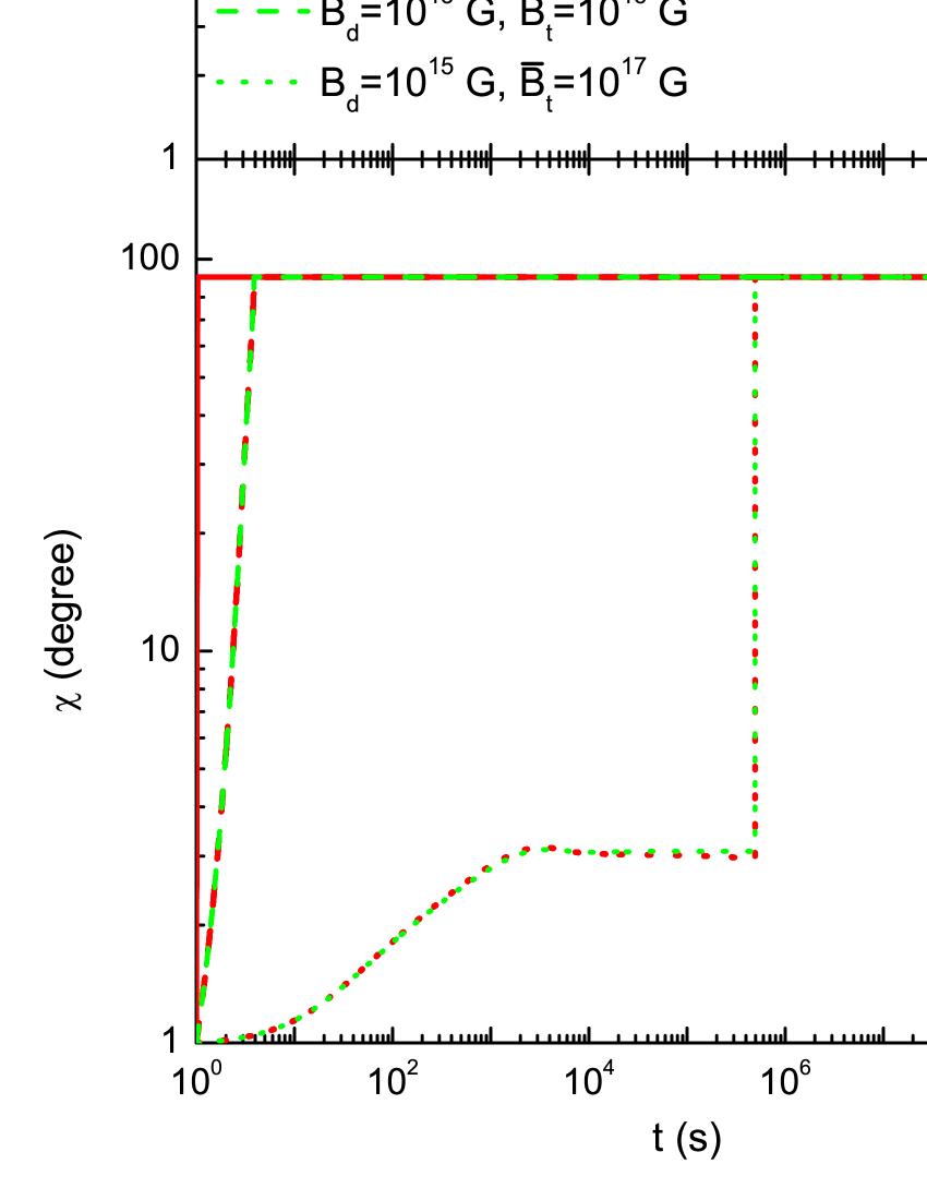
Figure 1: Evolutions of the spin frequency $\nu_{\rm NS}$ (upper panel) and tilt angle $\chi$ (lower panel) of newly born magnetars. The strengths of the surface dipole and the internal toroidal magnetic fields are shown in the legend. The initial conditions for the magnetars are $P_{\rm i}=1$ ms, $\chi_{\rm i}=1^{\circ}$, and $T_{\rm i}=10^{10}$ K. Other quantities for the magnetars are taken as $M=1.4M_{\odot}$, $R=10^{6}$ cm, and $I=10^{45}$ ${\rm g}~{}{\rm cm}^{2}$.

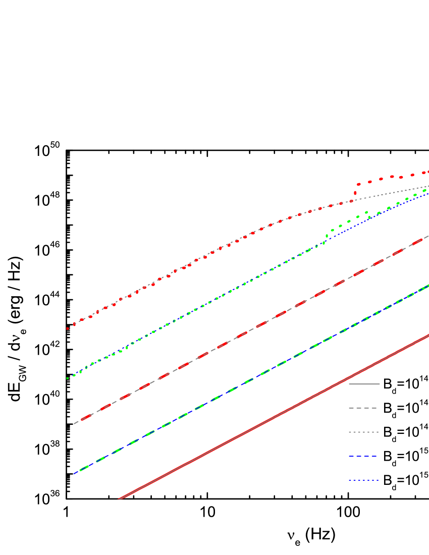
Figure 2: The GW energy spectra emitted by newly born magnetars with different strengths of the dipole and toroidal magnetic fields. The red and green lines represent the results calculated by involving the tilt angle evolutions. The dipole and toroidal fields are the same as those in Fig. 1. The grey and blue lines show the spectra derived only by assuming constant angles $\chi=\pi/2$, but with the same strengths of magnetic fields as in the cases of $\chi$ evolution, as shown in the legend.

With the above stellar evolutions, we show the corresponding GW radiation spectra in Fig. 2, where some results for constant tilt angles $\chi=\pi/2$ are also presented for comparisons. As shown, for ${\bar{B}}_{\rm t}\ll 10^{17}$ G, the influence of the tilt angle evolution on the GW radiation spectrum is very limited, since the angle changes too quickly. However, for ${\bar{B}}_{\rm t}=10^{17}$ G, some significant changes in the spectrum appear, in particular, in the high-frequency domain. To be specific, according to the contributor of radiation, the GW spectrum can be roughly divided into four segments. For instance, in the case of $B_{\rm d}=10^{14}$ G and ${\bar{B}}_{\rm t}=10^{17}$ G, following Equations (2) and (3), and defining $A={32\pi^{4}G\over 5c^{5}}I^{2}\epsilon_{\rm B}^{2}\nu_{\rm e}^{3}$, $B={B_{\rm d}^{2}R^{6}\over 6Ic^{3}}$, $C={2\pi^{2}G\over 5c^{5}}I\epsilon_{\rm B}^{2}\nu_{\rm e}^{2}$, we have

$$\frac{dE_{\rm gw}}{d\nu_{\rm e}}=\left\{\begin{aligned} &A{\rm sin}^{2}\chi[B+C(1+15{\rm sin}^{2}\chi)]^{-1},\cdots&\\ &1000<\nu_{\rm e}\leq 2000~{}{\rm Hz}&\\ &A{\rm cos}^{2}\chi[B+4C(1+15{\rm sin}^{2}\chi)]^{-1},\cdots&\\ &222\lesssim\nu_{\rm e}\leq 1000~{}{\rm Hz}&\\ &A{\rm cos}^{2}\chi[B+4C(1+15{\rm sin}^{2}\chi)]^{-1}\cdots&\\ &+A(B+16C)^{-1},~{}111\lesssim\nu_{\rm e}\lesssim 222~{}{\rm Hz}&\\ &A(B+16C)^{-1},~{}\nu_{\rm e}\lesssim 111~{}{\rm Hz}.&\\ \end{aligned}\right.$$ (7)

From the above equation we know that the first and fourth segments of the spectrum are contributed by the radiation at $2\nu_{\rm NS}$. While the second segment is dominated by the radiation at $\nu_{\rm NS}$ and the third part contains the contributions from $\nu_{\rm NS}$ and $2\nu_{\rm NS}$. On the other hand, the GW energy spectrum calculated for $\chi=\pi/2$ can be expressed as

$$\frac{dE_{\rm gw}}{d\nu_{\rm e}}=A(B+16C)^{-1},~{}\nu_{\rm e}\leq 2000~{}{\rm Hz}.$$ (8)

Dividing the four segments of Equation (7) with (8), respectively, one can see the GW radiation is reduced by ${B+16C\over B+C}{\rm sin}^{2}\chi\simeq 16{\rm sin}^{2}\chi$ (due to $B\ll C$) at the frequency band $1000<\nu_{\rm e}\leq 2000$ Hz; enhanced by ${B+16C\over B+4C}{\rm cos}^{2}\chi\simeq 4$ (due to $B\ll C$) at $222\lesssim\nu_{\rm e}\leq 1000$ Hz; enhanced by $4.4\lesssim 1+{B+16C\over B+4C}{\rm cos}^{2}\chi\lesssim 5$ (due to $B\ll C\rightarrow B\simeq C$) at $111\lesssim\nu_{\rm e}\lesssim 222$ Hz; unchanged at $\nu_{\rm e}\lesssim 111$ Hz as compared with the result derived by assuming $\chi=\pi/2$. These analytic results accurately account for the enhancement in the GW energy spectrum as shown in Fig. 2.

Likewise, in the case of $B_{\rm d}=10^{15}$ G and ${\bar{B}}_{\rm t}=10^{17}$ G, the GW energy spectrum could also be divided into four segments, namely, $1000<\nu_{\rm e}\leq 2000$ Hz, $140\lesssim\nu_{\rm e}\leq 1000$ Hz, $70\lesssim\nu_{\rm e}\lesssim 140$ Hz and $\nu_{\rm e}\lesssim 70$ Hz. From high- to low-frequency band the expression for each segment is the same as Equation (7). Owing to the rather small tilt angle at early period, the GW radiation is also suppressed at $1000<\nu_{\rm e}\leq 2000$ Hz. However, as $B_{\rm d}$ increases, much more rotational energy is released into MDR. Hence, the enhancement in the GW radiation is not as remarkable as in the previous case. Quantitatively, the GW energy spectrum is enhanced by $1\leq{B+16C\over B+4C}{\rm cos}^{2}\chi\lesssim 3.4$ ($B\lesssim C\rightarrow B\gg C$) and $1+{B+16C\over B+4C}{\rm cos}^{2}\chi\approx 2$ ($B\gg C$) at $140\lesssim\nu_{\rm e}\leq 1000$ Hz and $70\lesssim\nu_{\rm e}\lesssim 140$ Hz, respectively. Moreover, we confirmed the result of Marassi et al. (2011), which suggested that at low frequency band where MDR dominates the spin-down, the GW energy spectrum is reduced by two order of magnitudes while increasing $B_{\rm d}$ from $10^{14}$ to $10^{15}$ G.

3 Stochastic GW background

Generally, the SGWB is denoted by a dimensionless quantity, $\Omega_{\rm GW}(\nu_{\rm obs})$, which actually represents how the GW energy density is distributed with the frequency $\nu_{\rm obs}$ in the observer frame. Following Ferrari et al. (1999), this quantity takes the form

$$\Omega_{\rm GW}(\nu_{\rm obs})=\frac{1}{c^{3}\rho_{\rm c}}\nu_{\rm obs}F_{\nu}(\nu_{\rm obs}),$$ (9)

where $\rho_{\rm c}=3H_{0}^{2}/8\pi G$ is the critical energy density needed to close the universe. The GW flux at the observed frequency $\nu_{\rm obs}$ is

$$F_{\nu}(\nu_{\rm obs})=\int f_{\nu}(\nu_{\rm obs})dR(z),$$ (10)

where $f_{\nu}(\nu_{\rm obs})$ is the GW energy flux per unit frequency of a single source, $dR(z)$ is the magnetar formation rate located between $z$ and $z+dz$. The GW energy flux emitted by an single magnetar is related to its GW energy spectrum as (Regimbau & de Freitas Pacheco 2006a)

$$f_{\nu}(\nu_{\rm obs})=\frac{1}{4\pi d_{L}^{2}}\frac{dE_{\rm gw}}{d\nu_{\rm e}}(1+z),$$ (11)

where $d_{L}$ is the luminosity distance, and the GW frequency in the source frame has the form $\nu_{\rm e}=\nu_{\rm obs}(1+z)$.

The number of NSs formed per unit time out to redshift $z$ can be estimated by integrating the cosmic star formation rate (CSFR) density, $\dot{\rho}_{\ast}(z)$, over the comoving volume element, and taking into account the restriction associated with the initial mass function (IMF). Of all the NSs, $8-10\%$ are considered to be magnetars ($B_{\rm d}\geq 10^{14}$ G) according to the results of Regimbau & de Freitas Pacheco (2001) and Popov et al. (2009), who derived this ratio through population synthesis methods. In this paper, we assume the ratio to be $\xi=10\%$. As a consequence, the number of magnetars formed per unit time out to redshift $z$ within the comoving volume can be written as

$$R(z)=\xi\int_{0}^{z}\dot{\rho}_{\ast}(z^{\prime})\frac{dV}{dz^{\prime}}dz^{\prime}\int_{m_{\rm min}}^{m_{\rm max}}\Phi(m)dm,$$ (12)

where $dV/dz$ is the comoving volume element, and $\Phi(m)$ is the IMF. We take the CSFR density model suggested in Hopkins & Beacom (2006), which has refined the previous models up to redshift $z\sim 6$, and derived a parametric fit expression for the CSFR based on the new measurements of the galaxy luminosity function in the UV and far-infrared wavelengths. The CSFR density can be expressed as

$$\dot{\rho}_{\ast}(z)=h\frac{0.017+0.13z}{1+(z/3.3)^{5.3}}M_{\odot}{\rm yr}^{-1}{\rm Mpc}^{-3},$$ (13)

where $h=0.7$.

The comoving volume element in Equation (12) takes the following form (Regimbau & de Freitas Pacheco 2001, 2006a; Zhu et al. 2011)

$$\frac{dV}{dz}=4\pi\frac{c}{H_{0}}\frac{r(z)^{2}}{E(\Omega,z)},$$ (14)

where $E(\Omega,z)=\sqrt{\Omega_{m}(1+z)^{3}+\Omega_{\Lambda}}$, and $r(z)=d_{L}/(1+z)$ is the comoving distance, ${H_{0}}$ is the Hubble constant. We take the $\Lambda$CDM cosmological model with $H_{0}=70~{}{\rm km~{}s}^{-1}{\rm Mpc}^{-1}$, $\Omega_{m}=0.3$ and $\Omega_{\Lambda}=0.7$. The standard Salpeter IMF $\Phi(m)=Am^{-(1+x)}$ is adopted with $x=1.35$, where $A$ is a normalization constant, determined by the relation $\int_{0.1M_{\odot}}^{125M_{\odot}}m\Phi(m)dm=1$. It should be noted that the mass range of magnetar progenitor is still controversial (see Ferrario & Wickramasinghe 2008; Davies et al. 2009). However, we mainly focus on the effect of the tilt angle evolution on the resultant SGWB. For simplicity, we take the same mass range $m_{\rm min}=8M_{\odot}$, $m_{\rm max}=40M_{\odot}$ as Marassi et al. (2011) for the magnetar progenitors.

Combining the Equations (9), (10), (11), (12) and (14), one can obtain the SGWB contributed by the magnetically-induced deformation of an ensemble of newly born magnetars

$$\Omega_{\rm GW}(\nu_{\rm obs})=\frac{8\pi G\nu_{\rm obs}}{3H_{0}^{3}c^{2}}\int_{0}^{z_{\rm upp}}\frac{\dot{\rho}_{\ast}(z)}{(1+z)E(\Omega,z)}\frac{dE_{\rm gw}}{d\nu_{\rm e}}dz$$

$$\times\int_{m_{\rm min}}^{m_{\rm max}}\Phi(m)dm.$$ (15)

The upper limit of the redshift integration is determined by the maximal GW frequency in the source frame and the maximal redshift $z_{\ast}$ of the CSFR model. To be specific, $z_{\rm upp}=$min$(z_{\ast},\nu_{\rm e,max}/\nu_{\rm obs}-1)$. In deriving Equation (15), the time-dilation effect has been involved, so the term $(1+z)$ appears in the denominator.

4 RESULTS

In Fig. 3 we plot the dimensionless energy density $\Omega_{\rm GW}$ versus the observed frequency $\nu_{\rm obs}$ for newly born magnetars with different strengths of toroidal and dipole magnetic fields. Since for a magnetar with ${\bar{B}}_{\rm t}\ll 10^{17}$ G, its tilt angle evolution could not change the emitted GW energy spectrum, the background spectrum contributed by an ensemble of such magnetars is also unchanged even their angle evolution is involved. However, for newly born magnetars with ${\bar{B}}_{\rm t}=10^{17}$ G, the background spectra are obviously changed by the angle evolutions. These magnetars could keep rather small tilt angles for $\sim 5\times 10^{5}$ s, during which they have largely spun down. As a consequence, the GW radiation from $2\nu_{\rm NS}$ are seriously suppressed, resulting in the rather weak backgrounds above 1000 Hz. The background spectra show two cutoffs with frequencies at 1000 and 2000 Hz, respectively. Similar cutoffs are also presented in the spectrum contributed by magnetars with constant tilt angles $\pi/60$ (Marassi et al. 2011). Moreover, the background spectra contributed by newly born magnetars with ${\bar{B}}_{\rm t}=10^{17}$ G can also be divided into four segments.

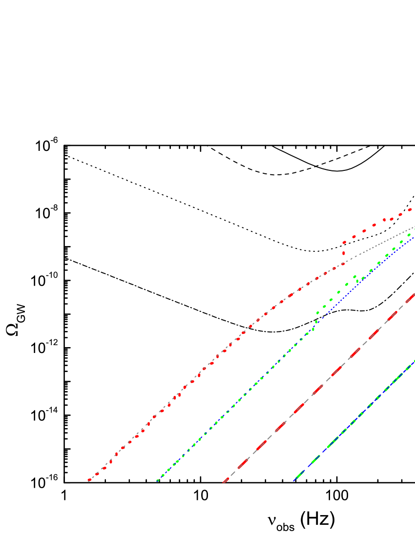
Figure 3: Dimensionless GW energy density $\Omega_{\rm GW}$ versus the observed frequency $\nu_{\rm obs}$ for newly born magnetars with different strengths of the dipole and toroidal magnetic fields, which are the same as in Figs. 1 and 2 (see the legends in these figures). The red and green lines represent the SGWBs calculated by involving the tilt angle evolutions. The grey and blue lines show the SGWBs derived only by assuming $\chi=\pi/2$, but with the same strengths of magnetic fields as in the cases of $\chi$ evolution. Please note that the background spectra contributed by magnetars with $B_{\rm d}=10^{14}$ G and ${\bar{B}}_{\rm t}=10^{15}$ G are not shown for both the $\chi$ evolution case and the $\chi=\pi/2$ case because they are too weak. The detection thresholds of LIGO (black solid line), VRIGO (black dashed line), aLIGO (black dotted line), and the proposed ET (black dash-dotted line), calculated using Equation (136) in Sathyaprakash & Schutz (2009) and assuming 1 yr observation time are also shown.

Specifically, for $B_{\rm d}=10^{14}$ G and ${\bar{B}}_{\rm t}=10^{17}$ G, the first segment of the spectrum is at the frequency band $1000<\nu_{\rm obs}\leq 2000$ Hz, the dimensionless energy density $\Omega_{\rm GW}$ is reduced by a factor $16{\rm sin}^{2}\chi$ compared with result of $\chi=\pi/2$. The evolution of $\Omega_{\rm GW}$ with $\nu_{\rm obs}$ above 1000 Hz is mainly due to the tilt angle evolution at early periods. Initially, the tiny angles lead to rather small $\Omega_{\rm GW}$ around 2000 Hz. Subsequently, as the tilt angles increase and then keep almost constant values of $3^{\circ}$, $\Omega_{\rm GW}$ increases and forms a plateau at $1000<\nu_{\rm obs}\lesssim 1250$ Hz. However, such an evolution behaviour of the background spectrum is unlikely to be detected currently. The second and third segments of the background spectrum are at the band $222\lesssim\nu_{\rm obs}\leq 1000$ Hz and $111\lesssim\nu_{\rm obs}\lesssim 222$ Hz, respectively. Quite the contrary, by involving the tilt angle evolution, $\Omega_{\rm GW}$ at the two bands are respectively increased by about 4, and $4.4-5$ times, following the analysis in Section 2. The enhanced SGWB could be detected by aLIGO at a few hecto-hertz. The main reason that leads to the enhancement is though the tiny tilt angle can suppress the GW radiation at $2\nu_{\rm NS}$ of a single magnetar, more rotational energy is released into GW with emitted frequency at $\nu_{\rm NS}$ instead. The fourth segment is at $\nu_{\rm obs}\lesssim 111$ Hz, which has no differences with that derived by assuming $\chi=\pi/2$.

The background spectrum produced by magnetars with $B_{\rm d}=10^{15}$ G and ${\bar{B}}_{\rm t}=10^{17}$ G also contains four segments, which are respectively $1000<\nu_{\rm obs}\leq 2000$ Hz, $140\lesssim\nu_{\rm obs}\leq 1000$ Hz, $70\lesssim\nu_{\rm obs}\lesssim 140$ Hz, and $\nu_{\rm obs}\lesssim 70$ Hz. Compared with the result of $\chi=\pi/2$, the first segment is also reduced by $16{\rm sin}^{2}\chi$, while the fourth segment keeps the same. Nevertheless, the second and third parts are enhanced by $\lesssim 3$ times and 2 times, respectively. Overall, stronger $B_{\rm d}$ could lead to much more rotational energy release in the form of MDR, rather than GW radiation, further result in a relatively weak SGWB. As shown in Fig. 3, the background produced by newly born magnetars with $B_{\rm d}=10^{15}$ G and ${\bar{B}}_{\rm t}=10^{17}$ G may only be detected by ET. Actually, if the GW radiation braking is dominative in the early spin evolution of the magnetars, the resultant background spectrum is relatively flat at a few tens to a few hundred hertz, because $dE_{\rm gw}/d\nu_{\rm e}\propto\nu_{\rm e}$ (GW radiation dominated) as compared to $dE_{\rm gw}/d\nu_{\rm e}\propto\nu_{\rm e}^{3}$ (MDR dominated) (Marassi et al. 2011).

One can expect that if all newly born magnetars indeed have ultra-strong toroidal magnetic fields of $10^{17}$ G, the resultant dimensionless GW energy densities would show sharp variations with the observed frequency at several tens to about 100 hertz. We suggest that if these features could be observed through precise detection of the SGWB by ET, it will provide us a key evidence about the early evolution of tilt angles. In addition, this would provide us some significant information about the properties of newly born magnetars, such as their braking, cooling mechanisms and the viscosity of nuclear matter. Of course, the current non-detection of the SGWB by aLIGO mainly has the following reasons: (i) not all newly born magnetars have ultra-strong toroidal magnetic fields of $10^{17}$ G; (ii) of all the newly born NSs, magnetars may have a ratio less than 10%; (iii) if all newly born magnetars have ${\bar{B}}_{\rm t}=10^{17}$ G, then most of them should have $B_{\rm d}=10^{15}$ G at least after their births.

5 CONCLUSION AND DISCUSSIONS

We have revisited the SGWB contributed by the magnetically-induced deformation of newly born magnetars involving the tilt angle evolutions based on the work of Dall’Osso et al. (2009). We find that for the magnetar with toroidal magnetic fields ${\bar{B}}_{\rm t}\ll 10^{17}$ G, its tilt angle evolution have no influence on the emitted GW energy spectrum. Hence, the SGWB from an ensemble of such magnetars is also unaffected by the angle evolution. However, for magnetars with ${\bar{B}}_{\rm t}=10^{17}$ G, their tilt angle evolutions could obviously change the GW energy spectra and the background spectra, which both could roughly be divided into four segments. Specifically, the background radiation above 1000 Hz are suppressed by a factor of $16{\rm sin}^{2}\chi$. The intermediate two segments range from $\sim 100-1000$ Hz, the background radiation of which are enhanced by about four times, and $4.4-5$ times for $B_{\rm d}=10^{14}$ G ($\lesssim 3$ times, and 2 times for $B_{\rm d}=10^{15}$ G), respectively. Since more rotational energy of the magnetars are released into MDR for higher $B_{\rm d}$, leading to the relatively weak enhancement in the GW background radiation. The last segments are at $\nu_{\rm obs}\lesssim 100$ Hz, the spectra of which are the same as the results of $\chi=\pi/2$. As a consequence, involving the tilt angle evolutions could result in some more stronger and detectable SGWBs, if the newly born magnetars indeed have ultra-strong toroidal magnetic fields. We expect that the evidence of tilt angle evolutions of newly born magnetars may possibly be found in their SGWBs. Moreover, sophisticated detection of the SGWB at the band below a few hundred hertz may put some constrains on the properties of these magnetars.

Finally, two aspects that may affect the tilt angle evolution should be considered in detail in future work. As we know, the bulk viscosity of quark matter is much larger than that of neutrons, protons and electrons nuclear matter. As a result, if the magnetars are quark stars or even hybrid stars, their tilt angle evolutions should be different from those of classical NSs considered in this paper. The resultant SGWBs are probably also different. On the other hand, the ellipticity and magnetic energy of the magnetar with ‘twisted-torus’ magnetic field configuration are different from that derived based on the toroidal-dominated configuration (Cutler 2002; Haskell et al. 2008; Ciolfi et al. 2009, 2010; Mastrano et al. 2011; Mastrano & Melatos 2012; Akgün et al. 2013; Mastrano et al. 2013; Mastrano et al. 2015). Hence, if the internal fields of magnetars indeed have a ‘twisted-torus’ shape, we may expect different tilt angle evolutions, which further result in various SGWBs.

ACKNOWLEDGEMENTS

We thank the anonymous referee for helpful discussions in improving this paper. This work is supported by the National Natural Science Foundation of China (grant nos 11133002, 11473008 and 11178001), the funding for the Authors of National Excellent Doctoral Dissertations of China (grant no. 201225), and the Program for New Century Excellent Talents in University (grant no. NCET-13-0822).

References

- [1] Abadie J., et al. 2011, Phys. Rev. D, 83, 042001
- [2] Abbott B. P., et al. 2010, ApJ, 713, 671
- [3] Akgün T., Reisenegger A., Mastrano A., Marchant P., 2013, MNRAS, 433, 2445
- [4] Alpar A., Sauls J. A., 1988, ApJ, 327, 723
- [5] Andersson N., 1998, ApJ, 502, 708
- [6] Bonazzola S., Gourgoulhon E., 1996, A&A, 312, 675
- [7] Braithwaite J., 2006, A&A, 449, 451
- [8] Braithwaite J., 2009, MNRAS, 397, 763
- [9] Braithwaite J., Spruit H. C., 2004, Nature, 431, 819
- [10] Braithwaite J., Spruit H. C., 2006, A&A, 450, 1097
- [11] Chamel N., Haensel P., 2008, Living Reviews in Relativity, 11, 10
- [12] Cheng Q., Yu Y. W., 2014, ApJL, 786, L13
- [13] Ciolfi R., Ferrari V., Gualtieri L., 2010, MNRAS, 406, 2540
- [14] Ciolfi R., Ferrari V., Gualtieri L., Pons J. A., 2009, MNRAS, 397, 913
- [15] Cutler C., 2002, Phys. Rev. D, 66, 084025
- [16] Cutler C., Jones D. I., 2001, Phys. Rev. D, 63, 024002
- [17] Dai Z. G., Lu T., 1998, Phys. Rev. Lett., 81, 4301
- [18] Dall’Osso S., Giacomazzo B., Perna R., Stella L., 2015, ApJ, 798, 25
- [19] Dall’Osso S., Shore S. N., Stella L., 2009, MNRAS, 398, 1869
- [20] Dall’Osso S., Stratta G., Guetta D., et al. 2011, A&A, 526, A121
- [21] Davies B., Figer D. F., Kudritzki R. P., Trombley C., Kouveliotou C., Wachter S., 2009, ApJ, 707, 844
- [22] Duncan, R. C., Thompson, C. 1992, ApJL, 392, L9
- [23] Ferrari V., Matarrese S., Schneider R., 1999, MNRAS, 303, 247
- [24] Ferrario L., Wickramasinghe D., 2008, MNRAS, 389, L66
- [25] Friedman J. L., Morsink S. M., 1998, ApJ, 502, 714
- [26] Haskell B., Samuelsson L., Glampedakis K., Andersson N., 2008, MNRAS, 385, 531
- [27] Hopkins A. M., Beacom J. F., 2006, ApJ, 651, 142
- [28] Inserra C., et al. 2013, ApJ, 770, 128
- [29] Jones P. B., 1976, Astrophys. Space Sci., 45, 669
- [30] Kasen D., Bildsten L., 2010, ApJ, 717, 245
- [31] Lai D., Shapiro S. L., 1995, ApJ, 442, 259
- [32] Marassi S., Ciolfi R., Schneider R., Stella L., Ferrari V., 2011, MNRAS, 411, 2549
- [33] Marranghello G. F., Vasconcellos C. Z., de Freitas Pacheco J. A., 2002, Phys. Rev. D, 66, 064020
- [34] Mastrano A., Lasky P. D., Melatos A., 2013, MNRAS, 434, 1658
- [35] Mastrano A., Melatos A., 2012, MNRAS, 421, 760
- [36] Mastrano A., Melatos A., Reisenegger A., Akgün T., 2011, MNRAS, 417, 2288
- [37] Mastrano A., Suvorov A. G., Melatos A., 2015, MNRAS, 447, 3475
- [38] Olausen S. A., Kaspi V. M., 2014, ApJS, 212, 6
- [39] Owen B. J., Lindblom L., Cutler C., Schutz B. F., Vecchio A., Andersson N., 1998, Phys. Rev. D, 58, 084020
- [40] Page D., Lattimer J. M., Prakash M., Steiner A. W., 2004, ApJS, 155, 623
- [41] Popov S. B., Pons J. A., Miralles J. A., Boldin P. A., Posselt B., 2009, MNRAS, 401, 2675
- [42] Regimbau T., Chauvineau B., 2007, Class. Quantum Grav., 24, 627
- [43] Regimbau T., de Freitas Pacheco J. A., 2001, A&A, 374, 182
- [44] Regimbau T., de Freitas Pacheco J. A., 2006a, A&A, 447, 1
- [45] Regimbau T., de Freitas Pacheco J. A., 2006b, ApJ, 642, 455
- [46] Rowlinson A., et al. 2013, MNRAS, 430, 1061
- [47] Sathyaprakash B. S., Schutz B. F., 2009, Living Reviews in Relativity, 12, 2
- [48] Schneider R., Ferrari V., Matarrese S., Potergies Zwart S. F., 2001, MNRAS, 324, 797
- [49] Sigl G., 2006, JCAP, 04, 002
- [50] Stella L., Dall’Osso S., Israel G. L., Vecchio A., 2005, ApJL, 634, L165
- [51] Stopnitzky E., Profumo S., 2014, ApJ, 787, 114
- [52] Yu Y. W., Cheng K. S., Cao X. F., 2010, ApJ, 715, 477
- [53] Yu Y. W., Dai Z. G., 2007, A&A, 470, 119
- [54] Zhang B., Mészáros P., 2001, ApJL, 552, L35
- [55] Zhu X. J., Fan X. L., Zhu Z. H., 2011, ApJ, 729, 59
- [56] Zhu X. J., Howell E. J., Blair D. G., Zhu Z. H., 2013, MNRAS, 431, 882