Discriminative Map Retrieval Using View-Dependent Map Descriptor

Abstract

Map retrieval, the problem of similarity search over a large collection of 2D pointset maps previously built by mobile robots, is crucial for autonomous navigation in indoor and outdoor environments. Bag-of-words (BoW) methods constitute a popular approach to map retrieval; however, these methods have extremely limited descriptive ability because they ignore the spatial layout information of the local features. The main contribution of this paper is an extension of the bag-of-words map retrieval method to enable the use of spatial information from local features. Our strategy is to explicitly model a unique viewpoint of an input local map; the pose of the local feature is defined with respect to this unique viewpoint, and can be viewed as an additional invariant feature for discriminative map retrieval. Specifically, we wish to determine a unique viewpoint that is invariant to moving objects, clutter, occlusions, and actual viewpoints. Hence, we perform scene parsing to analyze the scene structure, and consider the “center” of the scene structure to be the unique viewpoint. Our scene parsing is based on a Manhattan world grammar that imposes a quasi-Manhattan world constraint to enable the robust detection of a scene structure that is invariant to clutter and moving objects. Experimental results using the publicly available radish dataset validate the efficacy of the proposed approach.

Kondo Kensuke      Tanaka Kanji      Nagasaka TomomiThis work was partially supported by MECSST Grant in-Aid for Young Scientists (B) (23700229), by KURATA grants and by TATEISI Science And Technology Foundation. K. Kondo, K. Tanaka and T. Nagasaka are with Faculty of Engineering, University of Fukui, Japan. tnkknj@u-fukui.ac.jp

Figure 1: Local map descriptor (LMD). Unlike previous bag-of-words methods which ignore all information about the layout of local features, we develop a holistic descriptor that is view-dependent and highly discriminative. Our strategy is to explicitly model a unique viewpoint of an input local map; the pose of the local feature is defined with respect to this unique viewpoint, and can be viewed as an additional invariant feature for discriminative map retrieval. In the figure, from bottom to top, we observe an input pointset map, a result of scene parsing and viewpoint planning, a viewpoint-centric coordinate, and a set of visual words. Each visual word consists of an appearance word $w_{a}$ (vertical axis) and a pose word $\langle w_{x},w_{y}\rangle$ (horizontal axes), which is defined with respect to the planned viewpoint and viewing direction.

I Introduction

Map retrieval, the problem of similarity search over a large collection of local maps previously built by mobile robots, is crucial for autonomous navigation in indoor and outdoor environments. This study addresses a general map retrieval problem in which a 2D pointset map is provided as a query, and the system searches a size $N$ map database to determine similar database maps that are relevant under rigid transformation. One of the most popular approaches to address this problem is bag-of-words (BoW), a method derived from image retrieval techniques [1, 2, 3]. In BoW, a collection of local invariant appearance features (e.g., shape context [4], polestar [5]) is extracted from an input map and each feature is translated into a visual word. Consequently, an input map is described compactly and matched efficiently as an unordered collection of visual words, termed “bag-of-words” [1].

A major limitation of the BoW scene model is the lack of spatial information. The BoW methods ignore the spatial layout information of the features, and hence, they have severely limited descriptive ability [1]. Key relevant studies to address this issue include recent image retrieval techniques, such as spatial pyramid matching [6]. In such techniques, weak robust constraints are extracted from the spatial information, and are incorporated into the BoW model to significantly improve the discriminative power of the model. However, to apply such methods that were originally proposed for image data, we must first define the origin or viewpoint of an input map with respect to which the poses of local features are defined. This task is non-trivial because of the following reasons: (1) Unlike image data, map data lacks an explicit viewpoint; (2) Unlike image data, the area of a map is variable; it is incrementally updated by mapper robots and can grow in an unbounded manner.

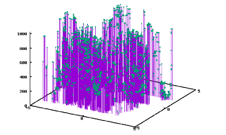
The main contribution of this study is an extension of the BoW map retrieval method to enable the use of spatial information from local features (Fig. 1). Our strategy is to explicitly model a unique viewpoint of an input local map; the pose of the local feature is defined with respect to this unique viewpoint, and can be viewed as an additional invariant feature for discriminative map retrieval. Specifically, we wish to determine a unique viewpoint that is invariant to moving objects, clutter, occlusions, and actual viewpoints. Hence, we perform scene parsing to analyze the scene structure, and consider the “center” of the scene structure to be the unique viewpoint. Our scene parsing is based on a Manhattan world grammar that imposes a quasi-Manhattan world constraint to enable the robust detection of a scene structure that is invariant to clutter and moving objects. We also discuss several strategies for extracting the “center” of a given scene structure. We generated a database of 2D local maps built by mobile robots from the publicly available radish dataset [7], and experimentally validated the efficacy of the proposed method.

I-A Related Work

Existing approaches to scene retrieval can be classified according to the feature descriptors used, the manner in which the feature descriptors are used, and whether the feature approach is global or local. A global feature approach describes the global structure of a scene by using a single global feature descriptor (e.g., Gist, HOG). In contrast, a local feature approach describes a scene by using a collection of local feature descriptors (e.g., SIFT). In general, both the approaches can be used complementarily; however, the focus of this paper is on the local feature approach.

Direct feature matching [8, 9, 10] and BoW [1, 2, 3] are two popular local feature approaches. In [8], the authors introduce the concept of RANSAC map matching for loop closure detection using pointset maps. In [9], the authors detect interest points, extract appearance descriptors (e.g., shape context), and perform a direct match between the appearance descriptors of the query and database images. Very recently, in [10] the authors presented an efficient direct matching based on multi-resolution many-to-many map matching framework. In [11], we also addressed the scalability issue by introducing a pre-filter based on the appearance descriptor. However, the direct matching methods have limited scalability because they require a large amount of time and space that is linearly proportional to the number of maps.

BoW methods [1, 2, 3] are well known for efficient map retrieval. In these methods, an input map is described compactly by an unordered collection of vector quantized appearance descriptors. In [12], we alse employed a bag-of-words scene model to achieve efficient visual robot localization. However, their descriptive ability is limited because they ignore all the layout information of the local features. We address this limitation in our study.

A majority of the existing BoW map retrieval methods explicitly or implicitly assume that the viewpoint trajectory of the mapper robot with respect to the local map is unavailable [1]. In contrast, we explicitly use the viewpoint information produced by our viewpoint planner as a cue to compute the local map descriptor. The success of our approach is based on the assumption that the viewpoint planner provides a unique viewpoint for a local map; therefore, we also consider viewpoint planning. These two issues have not been explored in existing literature.

Our study is also similar to several image retrieval techniques that describe the appearance and spatial information of local features. Among these methods, the part model [13], in which a scene is modeled as a collection of visual parts, is extremely popular. Spatial pyramid matching is an alternative method that places a sequence of increasingly coarser grids over the image region, and considers a weighted sum of the number of matches that occur at each level of resolution. However, most existing studies focus on image data, and do not handle map data that has no explicit viewpoint, as we discussed in Section I.

Our map parsing method can be viewed as an instance of scene parsing, which has been extensively studied in the fields of point-based geometry [14], image description [15], scene reconstruction [16], and scene compression [17]. Scene parsing approaches are broadly classified as generic approaches (e.g., line primitives [18], plane primitives [19], etc.) and parametric approaches (e.g., constructive solid geometry [20], hierarchical model [21], grammar-based [22], etc.). Our study can be viewed as a novel application of scene parsing to the map retrieval problem.

This study is a part of our studies on loop closure detection [23] and map-matching [24], and related to our previous works in ICRA15, IROS15, and PPNIV15 papers [12, 25, 26]. However, the use of viewpoint planning in map retrieval tasks is not addressed in existing studies.

II Map Retrieval Approach

For clarity of presentation, we first describe the overview of the map retrieval system that is the basis for our approach and is a performance comparison benchmark in the experiments described in Section IV. The main steps in the process are as follows: (1) Building informative local maps, (2) Planning the unique viewpoint of the local map, (3) Constructing a local map descriptor (LMD), and (4) Indexing/Retrieving the map database from the LMD descriptors. These four steps are explained below.

II-A Map Building

Based on existing literature [27], we build a local map from a short sequence of perceptual and odometry measurements; each measurement sequence must be sufficiently long to capture the rich appearance and geometric information of the local surroundings of the robot. In the implementation, each sequence corresponds to a 5 m run of the robot. Any map-building algorithm (e.g., FastSLAM, scan matching) can be used to register a measurement sequence to a local map. We start generating a local map every time the viewpoint of the robot moves 1 m along the path. Thus, a collection of overlapping local maps along the path is generated.

II-B Viewpoint Planning

In order to determine a unique viewpoint of a given input map that is invariant to moving objects, clutter, occlusions, and actual viewpoints, we first perform scene parsing to analyze the scene structure. Then, we consider the “center” of the scene structure to be the unique viewpoint. We will discuss several strategies for viewpoint planning in Section III. For example, in the strategy $S^{1}$, the scene structure is first analyzed to obtain a set of points, termed “structure points,” that belong to a structure (e.g., walls); then, the center-of-gravity of the structure points is computed, and finally, a nearest-neighbor unoccupied location relative to the center of gravity is determined as the unique viewpoint.

II-C Map Description

We follow a standard BoW approach [1] for extracting and representing appearance features. We adopt the polestar feature because it has several desirable properties, including viewpoint invariance and rotation independence, and has proven effective as a landmark for map matching in previous studies [28]. The extraction algorithm consists of three steps: (1) First, a set of keypoints is sampled from the raw 2D scan points. (2) Next, a circular grid is imposed and centered at each keypoint with different $D=10$ radius. (3) Finally, the points located in each circular grid cell are counted, and the resulting $D$-dim vector is generated as the output, the polestar descriptor. We quantize the appearance descriptor (i.e., $D$-dim polestar vector) of each feature to a 1-dimensional code termed an “appearance word”. This quantization process consists of three steps: (1) normalization of the $D$-dim vector by the L1 norm of the vector, (2) binarization of each $i$-th element of the normalized vector into $b_{i}\in\{0,1\}$, and (3) translation of the binarized $D$-dim vector into a code or a visual word, $w_{a}=\sum_{i}2^{i}b_{i}$. Currently, the threshold for binarization is determined by calculating the mean of all the elements of the vector. Thus, a map is represented by an unordered collection of visual words, $\{w_{a}~{}|~{}w_{a}\in[1,K]\}$, called BoW. We consider $D$-dim binarized polestar descriptors, and hence, the vocabulary size is $K=2^{10}$.

In order to translate the pose of each feature with respect to the planned unique viewpoint to a visual word, we quantize the pose or keypoint of the feature by using a resolution quantization step size of 0.1 m to obtain a code, $(w_{x},w_{y})$, termed “pose word”.

Finally, we obtain a BoW representation of the input local map, termed “local map descriptor (LMD)”. An LMD is an unordered collection of visual words, each having the form:

$$\langle w_{x},w_{y},w_{a}\rangle.$$ (1)

II-D Map Indexing/Retrieval

In order to index and retrieve the BoW map descriptors, we use the appearance word $w_{a}$ as the primary index for the inverted file system, and the pose word $(w_{x},w_{y})$ as an additional cue for fine matching. The retrieval stage begins with a search of the map collection. The given appearance word $w_{a}$ is used as a query to obtain all the memorized feature points with common appearance words, and to filter out the feature points whose pose word $(w_{x}^{\prime},w_{y}^{\prime})$ is distant from that of the query feature $(w_{x},w_{y})$:

$$|w_{x}-w_{x}^{\prime}|>D_{x,y},$$ (2)

$$|w_{y}-w_{y}^{\prime}|>D_{x,y}.$$ (3)

Thus, the final shortlist of maps is obtained. Currently, we use a large threshold, $D_{x,y}=3[m]$, to suppress false negatives, i.e., incorrect identification of relevant maps as not being relevant.

We use the BoW representation for the database construction and retrieval processes. In the database construction process, each local map is indexed by the inverted file system; each word $w_{a}$ belonging to the map is used as an index. In the retrieval process, all the indexes that have words in common with the query map are accessed, and the resulting candidate database maps are ranked based on the frequency or the number of words matched. For $K$ words in the vocabulary, a frequency histogram of visual words is represented by a $K$-dim vector.

[R1]                                       [R2]

[R3]                 [R4]                 [R5]

$$\mbox{[R1] }O\rightarrow M(\theta)^{*}$$

$$\mbox{[R2] }M(\theta)\rightarrow R_{x_{s},y_{s},\theta}(x_{s},y_{s},x_{e},y_{e})^{*}$$

$$\mbox{[R3] }R_{x,y,\theta}(x_{s},y_{s},x_{e},y_{e})\rightarrow R_{x,y,\theta}(x_{s},y_{s},x_{m},y_{e})R_{x,y,\theta}(x_{m},y_{s},x_{e},y_{e})$$

$$\mbox{[R4] }R_{x,y,\theta}(x_{s},y_{s},x_{e},y_{e})\rightarrow R_{x,y,\theta}(x_{s},y_{s},x_{e},y_{m})R_{x,y,\theta}(x_{s},y_{m},x_{e},y_{e})$$

$$\mbox{[R5] }R_{x,y,\theta}(a,b,c,d)\rightarrow\bar{W}_{x,y,\theta,a,b,c,b}\bar{W}_{x,y,\theta,c,b,c,d}\bar{W}_{x,y,\theta,c,d,a,d}\bar{W}_{x,y,\theta,a,d,a,b}$$

Figure 2: Manhattan world grammar and map parsing. Top: A Manhattan world grammar employing five rules, “[R1] initialize a Manhattan world,” “[R2] split a Manhattan world into rooms,” “[R3] split a room vertically,” “[R4] split a room horizontally,” and “[R5] split a room into four orthogonal walls.” Bottom: Map parsing algorithm. Examples of map parsing are shown in Fig. 3.

III Viewpoint Planning

In order to determine a unique viewpoint that is invariant to moving objects, clutter, and actual viewpoints, we first parse the scene structure using a Manhattan world grammar (Fig. 2), and then, determine the unique viewpoint with respect to the structure points. In the following subsections, first, we briefly introduce the Manhattan world grammar. Then, we describe the scene parsing algorithm, and discuss several strategies for viewpoint planning.

III-A Manhattan World Grammar

We use the formulation of context free grammar (CFG) to implement the Manhattan world grammar. CFG defines the grammar as

$$G=(V,T,R,U),$$ (4)

where $V$ is a set of non-terminal nodes. Each non-terminal node is represented by a capital letter, etc. $T$ is a set of terminal nodes. Each terminal node is represented by a capital letter with a bar over it, e.g., ’$\bar{A}$’, ’$\bar{B}$’, ’$\bar{C}$’, etc.

In the case of a map parsing problem, either a terminal or a non-terminal node is modeled as a geometric primitive; in our study, we use a “room” or “wall” primitive. $R$ is a set of replacement rules. Each replacement rule $r\in R$ is in the form

$$A\rightarrow a$$ (5)

and replaces a non-terminal node $A$ with a sequence of terminal or non- terminal nodes $a$. $U$ is the start variable. Let constant $N$ denote the upper bound on the number of grammar rules applied in a map parsing task. Let variable $r_{i}$ denote the $i$-th rule in the length $N$ rule sequence. The solution space of a map parsing problem is defined as

$$p=\{(r_{1},r_{2},\cdots,r_{N})\}.$$ (6)

The score $S(p)$ $(p\in P)$ of a policy $p$ is evaluated in terms of how well the original input map is explained by a set of primitives (i.e., terminal nodes) produced by the rule sequence $p$. The objective of a map parsing problem is to find a “best” policy $p^{best}(\in P)$ that maximizes the score function $S(p)$. In our method, the score $S(p)$ is evaluated in terms of the ratio of datapoints that are explained by the rule sequence $p$: $Size(O\setminus O^{c})/Size(O)$, where $Size(\cdot)$ is the number of datapoints, $O$ is the set of datapoints in the input map, and $O^{c}(\subset O)$ is a subset that is explained by the grammar $p$.

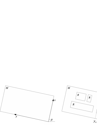
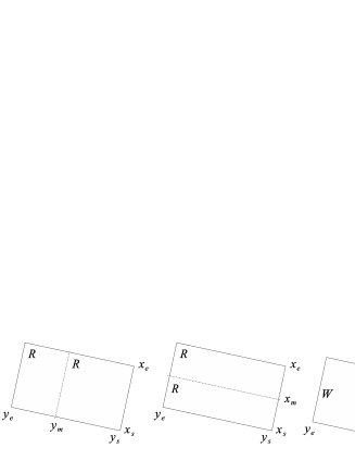
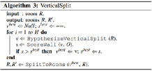
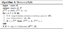
In order to adapt CFG to our map parsing method, we model the entire map as a set of “Manhattan worlds,” and “rooms” and “walls”. A Manhattan world [29] is a set of rectangular rooms aligned with the orthogonal directions. A room is composed of a set of four orthogonal walls. A wall is represented by a 2D line segment. The grammar is represented by a set of rules, R1, R2, R3, R4, and R5. Figure 2 illustrates each rule and its parameter settings. The symbol $O$ represents the original pointset map. A Manhattan world $M(\theta)$ is explained by a collection of orthogonal room primitives and is oriented at angle $\theta$. A room primitive $R_{\theta}(x,y,w,h)$ is explained by smaller orthogonal rooms or a set of four orthogonal walls. The angle, width, and height of a room primitive are $\theta$, $w$ and $h$, respectively. A wall primitive $\bar{W}_{x,y,\theta,a,b,c,d}$ is represented by a straight line segment, which is the result of rotating a line segment $(a,b)$-$(c,d)$ by angle $\theta$ around the point $(x,y)$.

a

b

c

Figure 3: Examples of viewpoint planning. Each panel shows the scene parsing for the query map (left) and the relevant database map (right). We performed scene parsing using Manhattan world grammar and obtained “wall” primitives and unoccupied regions, as shown in the figures. The red rectangles are the bounding boxes generated by strategy $S^{5}$.

III-B Map Parsing

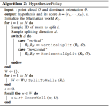
Our method for determining a best policy uses a hypothesize-and-verify approach. Given an input pointset map, we wish to determine a policy that maximizes a pre-defined score function $p^{best}(\in P)$. Our approach first estimates the dominant orientation $\theta$ of the Manhattan world; then, it generates $K$ random hypotheses for the policy, assigns a score to each hypothesis, and selects the hypothesis with the highest score as the best policy. The above methods for estimating the dominant orientation, generating hypotheses, and assigning a score to the hypotheses are explained in algorithms I-IV in Fig. 2. As mentioned, the score $S(\cdot)$ of a policy hypothesis is defined by the number of datapoints that would be explained by the policy. A data-driven algorithm is used for policy generation and evaluation.

III-C Viewpoint Planning

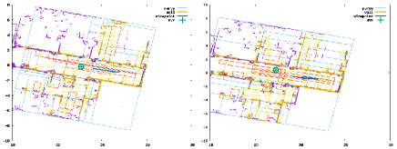
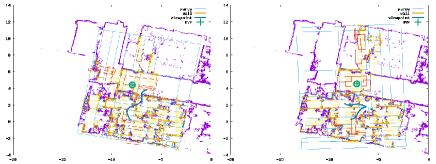
Given a scene understanding from the grammar-based parsing, we identify the “center” of a map and use it as the unique viewpoint (UVP), as shown in Fig. 3. In this study, we implement five strategies, $S^{1}$-$S^{5}$, to identify the center of a given input map, and experimentally evaluate the effectiveness of each strategy in terms of “viewpoint uniqueness” and map retrieval performance.

In this subsection, we use the following technical terms: grid map, free cells, unknown cells, wall cells, structure cells, and unoccupied cells. A grid map is a classical representation of a map that imposes a discretized grid on the $xy$-plane and classifies each cell as occupied, free, or unknown [30]. We denote occupied, free, and unknown cells as $C^{occupied}$, $C^{free}$ and $C^{unknown}$, respectively. The grid map is constructed during the map building process described in Section II-A. In addition, wall, structure, and unoccupied cells are defined based on the three cell classes mentioned above. Wall cells, $C^{wall}$, are the cells that are occupied by the wall primitives defined in Section III-A. Structure cells, $C^{structure}$, are defined as $C^{structure}=C^{occupied}\cap C^{wall}$. Unoccupied cells, $C^{unoccupied}$ are defined as $C^{unoccupied}=C^{free}\setminus C^{structure}$.

The strategy $S^{1}$ determines UVP as an unoccupied location near the center-of-gravity of structure points. First, $S^{1}$ parses the scene structure and obtains a set of wall points; then, it computes structure points $C^{structure}=\{(x_{i},y_{i})\}_{i=1}^{N}$ from the wall points and occupied cells as shown above, and, based on the result, it computes the center-of-gravity of the structure points $p^{cog}=N^{-1}\sum_{i=1}^{N}[x_{i}~{}y_{i}]^{T}$. Finally, it searches the unoccupied cells and determines a nearest-neighbor unoccupied cell relative to the center-of-gravity to be UVP: $p^{uvp}=\arg\min_{v\in C^{unoccupied}}|v-p^{cog}|$.

The strategy $S^{2}$ determines UVP as an unoccupied cell that minimizes the distance to the farthest structure points. Similar to the strategy $S^{1}$, $S^{2}$ parses the scene structure to obtain the structure and unoccupied cells. Then, for each viewpoint candidate $v$ (i.e., unoccupied cell), $S^{2}$ evaluates the distance $d(v)=\max_{p\in C^{structure}}|v-p|$ between the viewpoint and its farthest structure point, and selects one candidate that minimizes the evaluated distance: $p^{uvp}=\arg\min_{v\in C^{unoccupied}}d(v)$.

The strategy $S^{3}$ determines UVP as an unoccupied cell that maximizes the distance to the nearest structure points. The process for viewpoint planning is similar to that in $S^{2}$. The only difference is that $S^{3}$ uses the minimum distance instead of the maximum distance, and the maximum operator instead of the minimum operator, i.e., $d(v)=\min_{p\in C^{structure}}|v-p|$, and $p^{uvp}=\arg\max_{v\in C^{unoccupied}}d(v)$.

The strategy $S^{4}$ is based on the analysis of dominant structures, which are defined as the longest line segments on the input map. This strategy is similar to $S^{1}$; however, instead of using every structure point, $S^{4}$ uses only the 10 longest walls to compute the structure cells.

The strategy $S^{5}$ determines UVP as the center of the unoccupied regions. In the viewpoint planning process, $S^{5}$ searches a set of bounding boxes of unoccupied cells aligned with the orthogonal directions of the Manhattan world; then, it generates two histograms $f^{x},f^{y}$ of unoccupied cells along two dominant directions of the Manhattan world. Next, the peaks $x^{*}=\arg\max_{x}f^{x}(x)$ and $y^{*}=\arg\max_{y}f^{y}(y)$ of the two histograms are searched. Further, a bounding box of unoccupied cells $(x,y)$ whose $f^{x}(x)$ and $f^{y}(y)$ values exceed $0.9f^{x}(x^{*})$ and $0.9f^{y}(y^{*})$, respectively, is computed. Finally, UVP is defined as the center of the bounding box.

Figure 4: Datasets used in the experiments: “albert,” “fr079,” “run1,” “fr101,” “claxton,” and “kwing” from the radish dataset [7].

Figure 5: Examples of map retrieval. From left to right, a query map, the ground-truth database map, map retrieved by BoW method, and map retrieved by strategy $S^{5}$.

IV Experiments

We conducted map retrieval experiments to verify the efficacy of the proposed approach. In the following subsections, first, we describe the datasets and the map retrieval tasks used in the experiments; then, we present the results and compare the performance of our method with that of other methods.

IV-A Dataset

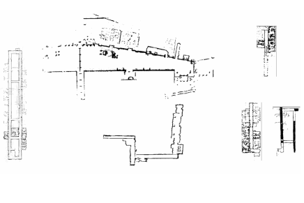
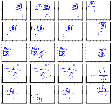
For map retrieval, we created a large-scale map collection from the publicly available radish dataset [7], which comprises odometry and laser data logs acquired by a car-like mobile robot in indoor environments (Fig. 4). We used a scan matching algorithm to create a collection of query-database maps from each of six datasets —“albert,” “fr079,” “run1,” “fr101,” “claxton,” and “kwing”— that were obtained from 212, 209, 80, 277, 79, and 286 m travel of the mobile robot, corresponding to 4167, 3118, 2882, 5299, 4150, and 609 scans. Fig. 5 shows examples of the query and database maps. The map collection comprises more than 1065 maps. Our map collections contain many virtually duplicate maps, thus making map retrieval a challenging task. We use “claxton” only as additional distructer maps for increasing the database size, as “claxton” does not contain any loop closure.

IV-B Qualitative Results

The objective of map retrieval is to find a relevant map from the map database for a local map given as a query. The relevant map is defined as a database map that satisfies two conditions: (1) Overlap of datapoints between the query and the relevant maps exceeds $R^{overlap}=75\%$, and (2) Its distance traveled along the robot’s trajectory is distant from that of the query map, such as in a “loop-closing” situation in which a robot traverses a loop-like trajectory and returns to a previously explored location.

For each relevant map pair, map retrieval is performed using a query map and a size $N$ map database, which consists of the relevant map and $(N-1)$ random irrelevant maps. The spatial resolution of the occupancy map is set to 0.1 m. We implemented the map retrieval algorithm in C++, and successfully tested it with various maps. Fig. 5 shows the results of map retrieval performed using the baseline (“BoW”) and the proposed (“LMD”) systems. As described in Section II, BoW differs from LMD only in that it does not use pose word but only uses appearance word. It is observed that the proposed LMD method yields fewer false positives than the BoW method. The reason for this result is that, in the proposed LMD method, many incorrect matches are successfully filtered out by the proposed descriptor, which uses the keypoint configuration as a cue. It can be observed that, for these examples, the proposed LMD method using the spatial layout of local features as a cue is successful in finding relevant maps.

TABLE I: Summary of ANR Performance [%]

dataset	albert	fr079	fr101	kwing1	run1	Avg
BoW	26.3	21.4	25.0	32.3	33.8	24.8
$S^{1}$	23.3	18.1	21.5	17.8	19.0	20.2
$S^{2}$	24.9	9.4	28.6	27.0	27.7	18.6
$S^{3}$	32.3	37.2	41.3	46.5	47.6	37.4
$S^{4}$	15.2	10.0	23.8	21.5	35.9	15.5
$S^{5}$	17.6	13.1	20.4	21.4	34.8	16.6

Figure 6: Performance in normalized rank [%].

IV-C Quantitative Results

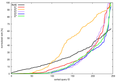
For performance comparison, we evaluated the averaged normalized rank (ANR) [24] for the BoW and LMD methods. ANR is a ranking-based performance measure in which a lower value is better. In order to determine the ANR, we performed several independent map retrieval tasks with various queries and databases. For each task, the rank assigned to the ground-truth database map by a map retrieval method of interest was investigated, and the rank was normalized by the database size $N$. The ANR was subsequently obtained as the average of the normalized ranks over all the map retrieval tasks. All map retrieval tasks were conducted using 247 different queries and a size 1065 map database.

Table I and Fig. 6 summarize the ANR performance. The proposed LMD system with strategies $S^{1}$, $S^{2}$, $S^{4}$, and $S^{5}$ clearly outperforms the baseline BoW system. An exception is the strategy $S^{3}$ and will be discussed in the next subsection, Section IV-D. By filtering out incorrect matches using the keypoint configuration as a cue, the LMD method was able to successfully perform map retrieval in many cases, as shown in the table. In contrast, the BoW system based only on appearance words does not perform well in many cases, mainly owing to the large number of false matches. The above results verify the efficacy of our approach.

IV-D Comparing Different Strategies

Table I also compares different viewpoint planning strategies for the proposed LMD algorithm. One can see that $S^{4}$ and $S^{5}$ are best strategies in the current experiment. The strategy $S^{4}$ is based on dominant structure in the map and it was successful in finding center of structures. The strategy $S^{5}$ is based on analysis of unoccupied regions and it was often successful in finding center of unoccupied regions. On the other hand, $S^{3}$ was not as good as other strategies and the BoW method. A main reason is that because $S^{3}$ maximizes the distance from UVP to the nearest structure points, it often determines UVP near the boundary between free and unknown region, which is naturally far apart from the center of the map. On the other hand, $S^{2}$ provided a good result as it minimizes the distance from UVP to the farthest structure points, which is often located at the center of a map. Finally, $S^{1}$ uses all the datapoints in a map and tends to be influenced by non-structure points and noises, and as a result, it performs not as good as $S^{4}$.

Figure 7: Histogram of errors in viewpoint planning.

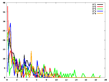
IV-E Viewpoint Planning

In this subsection, we investigate the performance of our viewpoint planning method. As mentioned earlier, the success of our approach is based on the assumption that the viewpoint planner provides a unique viewpoint for a given local map. As a proof-of-concept experiment, we investigate the similarity between the planned viewpoints of the query and those of the relevant database maps. We performed viewpoint planning for the 247 pairs of query and relevant maps, and computed the errors in the viewpoints planned. Fig. 7 shows a summary of the investigation in the form of a histogram. The difference between the planned viewpoint of the query and that of the relevant database maps was, for 90% of the viewpoints considered in the current study, within 5 m, 7.8 m, 12 m, 6.2 m, and 6.4 m for strategies $S^{1}$-$S^{5}$, respectively.

IV-F Matching Visual Words

$S^{5}$

$S^{1}$

BoW

Figure 8: Examples of matching visual words between relevant map pairs. Red lines connect matched visual words between query and relevant database maps.

$S^{5}$

$S^{1}$

BoW

Figure 9: Examples of matching visual words between irrelevant map pairs.

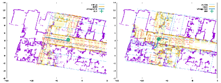
Figs. 8 and 9 show the results of matching visual words using the baseline (“BoW”) and the proposed (“LMD”) systems. In these figures, purple and green points indicate the query and the database maps, while the red lines indicate correspondence found by either method. To facilitate visualization, both maps are aligned w.r.t. the true viewpoints. With the above visualization, one can recognize false positive matches produced by either BoW or LMD method as they appear as relatively long red line segments that connect wrong pairs of datapoints between query and database maps. One can see that LMD methods provide significantly less amount of matches for irrelevant pairs than for relevant pairs comparing to BoW method.

TABLE II: Performance for dissimilar map pairs in ANR [%]

dataset	albert	fr079	fr101	kwing1	run1	Avg
BoW	24.6	22.6	21.7	55.8	36.6	25.4
$S^{1}$	12.3	10.3	18.9	31.6	30.0	14.4
$S^{2}$	20.7	11.3	28.8	29.3	26.3	19.4
$S^{3}$	33.6	34.8	39.8	45.0	51.2	36.3
$S^{4}$	13.8	11.2	23.0	42.2	41.7	16.9
$S^{5}$	15.7	14.5	17.4	32.3	36.6	16.9

IV-G Dissimilar Map Pairs

As a final investigation, we conducted an additional experiments on a challenging map retrieval scenario. In this study, we are interested in how robust individual map retrieval algorithms are and how well they perform on retrieving dissimilar maps. To this end, we use a lower threshold of overlap $R^{overlap}=50\%$, instead of the previous setting $R^{overlap}=75\%$. Table II reports the ANR performance. The strategies $S^{4}$ and $S^{5}$ again performed well and $S^{1}$ was best performed in this case. We can observe that despite the challenging setting, the proposed algorithm is still successful in viewpoint planning and map retrieval.

V Conclusions

In this study, we focused on a method that extends BoW map retrieval to enable the use of spatial information from local features. Our strategy is to explicitly model a unique viewpoint of an input local map; the pose of the local feature is defined with respect to this unique viewpoint, and can be viewed as an additional invariant feature for discriminative map retrieval. Specifically, we wish to determine a unique viewpoint that is invariant to moving objects, clutter, occlusions, and actual viewpoints. Hence, our approach employs scene parsing to analyze the scene structure, and the “center” of the scene structure is determined to be the unique viewpoint. Our scene parsing method is based on a Manhattan world grammar that imposes a quasi-Manhattan world constraint to enable the robust detection of a scene structure that is invariant to clutter and moving objects. We have also discussed several strategies for viewpoint planning that are based on different definitions of the “center” of a map. Experimental results using the publicly available radish dataset validate the efficacy of the proposed approach.

References

- [1] M. Cummins and P. Newman. Appearance-only slam at large scale with fab-map 2.0. Int. J. Robotics Research, 30(9):1100–1123, 2011.
- [2] Jan Knopp, Josef Sivic, and Tomas Pajdla. Avoiding confusing features in place recognition. In ECCV, pages 748–761. 2010.
- [3] Panu Turcot and David G Lowe. Better matching with fewer features: The selection of useful features in large database recognition problems. In Computer Vision Workshops (ICCV Workshops), 2009 IEEE 12th International Conference on, pages 2109–2116. IEEE, 2009.
- [4] Mori G., Belongie S., and Malik J. Shape contexts enable efficient retrieval of similar shapes. Proc. IEEE Computer Vision and Pattern Recognition, pages 723–730, 2001.
- [5] E. Silani and M. Lovera. Star identification algorithms: Novel approach & comparison study. IEEE Trans. Aerospace and Electronic Systems, 42(4):1275–1288, 2006.
- [6] Svetlana Lazebnik, Cordelia Schmid, Jean Ponce, et al. Spatial pyramid matching. Object Categorization: Computer and Human Vision Perspectives, 3:4, 2009.
- [7] Andrew Howard and Nicholas Roy. The robotics data set repository (radish), 2003.
- [8] Neira J., Tardos J.D., and Castellanos J.A. Linear time vehicle relocation in slam. Proc. IEEE Int. Conf. Robotics and Automation, 1:427– 433, 2003.
- [9] Gian Diego Tipaldi and Kai O Arras. Flirt-interest regions for 2d range data. In Robotics and Automation (ICRA), 2010 IEEE International Conference on, pages 3616–3622. IEEE, 2010.
- [10] Edwin Olson. M3RSM: many-to-many multi-resolution scan matching. In IEEE International Conference on Robotics and Automation, ICRA 2015, Seattle, WA, USA, 26-30 May, 2015, pages 5815–5821, 2015.
- [11] K. Saeki, K. Tanaka, and T. Ueda. Lsh-ransac: An incremental scheme for scalable localization. Proc. IEEE Int. Conf. Robotics and Automation, pages 3523–3530, 2009.
- [12] Tanaka Kanji. Cross-season place recognition using nbnn scene descriptor. In Intelligent Robots and Systems, 2015 IEEE/RSJ International Conference on. IEEE, 2015.
- [13] Dongfeng Han, Wenhui Li, and Zongcheng Li. Semantic image classification using statistical local spatial relations model. Multimedia Tools Appl., 39(2):169–188, 2008.
- [14] Ruwen Schnabel and Reinhard Klein. Octree-based point-cloud compression, 2006.
- [15] B.Z. Yao, X. Yang, L. Lin, M.W. Lee, and S.C. Zhu. I2t: Image parsing to text description. 98(8):1485–1508, 2010.
- [16] Peter Wonka, Michael Wimmer, François Sillion, and William Ribarsky. Instant architecture. ACM Transaction on Graphics, 22(3):669–677, 2003.
- [17] Alexander Toshev, Philippos Mordohai, and Ben Taskar. Detecting and parsing architecture at city scale from range data. Computer Vision and Pattern Recognition, IEEE Computer Society Conference on, 0:398–405, 2010.
- [18] Stephan Scholze, Theo Moons, and Luc J. Van Gool. A probabilistic approach to building roof reconstruction using semantic labelling. Proc. the 24th DAGM Symposium on Pattern Recognition, pages 257–264, 2002.
- [19] Zuwhan Kim and Ramakant Nevatia. Automatic description of complex buildings from multiple images. Comput. Vis. Image Underst, 96:2004, 2004.
- [20] Mathieu Brédif, Didier Boldo, Marc Pierrot Deseilligny, and Henri Maître. 3d building reconstruction with parametric roof superstructures, 2007.
- [21] Sung Chun Lee and Ram. Nevatia. Interactive 3d building modeling using a hierarchical representation. Proc. the First IEEE International Workshop on Higher-Level Knowledge in 3D Modeling and Motion Analysis, pages 58–, 2003.
- [22] Pascal Müller, Peter Wonka, Simon Haegler, Andreas Ulmer, and Luc Van Gool. Procedural modeling of buildings. ACM Trans. Graph., 25:614–623, 2006.
- [23] Tanaka K and Kondo E. Incremental ransac for online vehicle relocation in large dynamic environments. Proc. IEEE Int. Conf. Robotics and Automation, pages 1025–1030, 2006.
- [24] Hanada Shogo and Tanaka Kanji. Partslam: Unsupervised part-based scene modeling for fast succinct map matching. In IEEE/RSJ Int. Conf. IROS, pages 1582–1588. IEEE, 2013.
- [25] Masatoshi Ando, Yuuto Chokushi, Kanji Tanaka, and Kentaro Yanagihara. Leveraging image-based prior in cross-season place recognition. In ICRA, 2015.
- [26] Liu Enfu and Tanaka Kanji. Discriminative map matching using view dependent map descriptor. In IROS15 WS PPNIV, 2015.
- [27] Lina M Paz, Pedro Piniés, Juan D Tardós, and José Neira. Large-scale 6-dof slam with stereo-in-hand. Robotics, IEEE Transactions on, 24(5):946–957, 2008.
- [28] Kanji Tanaka and Kensuke Kondo. Multi-scale bag-of-features for scalable map retrieval. JACIII, 16(7):793–799, 2012.
- [29] James M Coughlan and Alan L Yuille. Manhattan world: Compass direction from a single image by bayesian inference. In Computer Vision, 1999. The Proceedings of the Seventh IEEE International Conference on, volume 2, pages 941–947. IEEE, 1999.
- [30] Sebastian Thrun, Wolfram Burgard, and Dieter Fox. Probabilistic robotics. MIT press, 2005.