Exploring the Parameter Space of Warm-Inflation Models

Abstract

Warm inflation includes inflaton interactions with other fields throughout the inflationary epoch instead of confining such interactions to a distinct reheating era. Previous investigations have shown that, when certain constraints on the dynamics of these interactions and the resultant radiation bath are satisfied, a low-momentum-dominated dissipation coefficient $\propto T^{3}/m_{\chi}^{2}$ can sustain an era of inflation compatible with CMB observations. In this work, we extend these analyses by including the pole-dominated dissipation term $\propto\sqrt{m_{\chi}T}\exp(-m_{\chi}/T)$. We find that, with this enhanced dissipation, certain models, notably the quadratic hilltop potential, perform significantly better. Specifically, we can achieve 50 $\mathrm{e}$-folds of inflation and a spectral index compatible with Planck data while requiring fewer mediator field ($\mathcal{O}(10^{4})$ for the quadratic hilltop potential) and smaller coupling constants, opening up interesting model-building possibilities. We also highlight the significance of the specific parametric dependence of the dissipative coefficient which could prove useful in even greater reduction in field content.

1 Introduction

Recent CMB data has made it evident that dissipation and particle production may have a role to play in the inflationary phase. The lack of detection of a tensor mode has meant that now the tensor-to-scalar ratio is low enough to rule out two of the most compelling cold-inflation models, the chaotic $\phi^{2}$ and $\phi^{4}$ inflation models [1, 2, 3, 4, 5, 6]. Of course, various fix-ups to these models are possible that have some limited success [7, 8, 4, 5, 9], but the basic argument that has kept these models in favor, that of simplicity, has now been lost. The warm inflation realization of both these models allows the tensor-to-scalar ratio to go down to levels constrained by CMB data, although only the $\phi^{4}$ model is also consistent with the bounds on tilt [10, 11, 12].

The warm-inflation realization of these models relies on the coupling of the inflaton to other fields, and the subsequent non-equilibrium dissipative dynamics that develop from these interactions, leading to particle production during inflation and to thermal seeds of density perturbations. Of course, the inflaton field is always coupled to other fields [13, 14, 15, 16, 17, 18, 19, 20]. Even in cold inflation, this is necessary for the reheating phase that is meant to follow inflation. Nevertheless, warm inflation is rather more technically complicated than generic cold inflation models. This is because in warm inflation the quantum-field-theory dynamics of particle production must coincide with inflation, which imposes various demands on the underlying dynamics [21, 22, 23]. However, from a theoretical perspective, the couplings in these warm-inflaton realizations are generic and, aside from requiring global SUSY to cancel radiative corrections, no other new physics is required beyond what has already been tested and verified in collider experiments. Cold inflation realizations of the chaotic models now consistent with CMB data require more novel new physics, adjusting the nature of gravity such as in the Higgs inflation model [7, 24] and other models involving non-minimal coupling [8, 25]. Other cold inflation models which have become popular since recent CMB data, such as the Starobinsky model [26], also require rather novel speculations about the nature of gravity at high energies. The difficulty with such models is, they are quite contrived, thus have limited scope for predictiveness. On the other hand, warm-inflation models don’t make radical demands on new physics but are quite complex. What is clear though, that neither of the two options between warm- and cold-inflation dynamics is more compelling at this stage. And whereas cold-inflation models have been exhaustively studied over three decades by many authors, there has been relatively little study of warm inflation.

In this paper, we will examine a variety of warm-inflation models and test their agreement with observation. There have been various studies of warm-inflation models and their observational predictions. One of the features of warm-inflation models constructed from first-principles quantum field theory has been that after all the constraints are applied, the models usually work at very high field content. The reason for this is not, as one might naively assume, that more fields implies more channels for dissipation, thus more radiation. Instead, large numbers of fields arise from requiring the first-principles model to satisfy both the usual observational constraints and consistency constraints from the field theory. The success of warm inflation models with the observational data is a significant result, but now we would like to further understand the underlying dynamics and the constraints involved and see if better parametric regimes can be obtained, in particular with lower number of fields required, to realize observationally consistent warm inflation.

This paper will therefore attempt a more in-depth analysis of the parameter space in a variety of warm-inflation models based on monomial, hybrid, and hilltop potentials with different powers of the inflaton field. For this, we will use numerical algorithms that allow exploration of the parameter space in search of regimes consistent with observation and the theoretical constraints.

We will scan over the 6-dimensional parameter space that sets the coupling constants and field content of these models as well as the initial conditions for radiation-density and inflaton evolution. For each randomly generated combination of these parameters, we check the conditions necessary for slow-roll and for warm inflation; we then integrate the coupled set of evolution equations for the inflaton, the radiation density, and the scale factor until any of these conditions break down or until the radiation density comes to dominate over the potential energy of the inflaton.

In section 2 we briefly introduce the dynamics of warm inflation with a general dissipation coefficient; a more thorough review can be found in ref. [23]. Section 3 presents the spectral index and the tensor-to-scalar ratio for this class of models; our models’ predictions for these observables will be fundamental to our comparison to Planck results in later sections. Section 4 argues that for certain powers of the inflaton field in the potential, the ratio between the field value and the temperature is constant during slow-roll; these models then form part of the numerical investigations we describe in section 5. We present our results and conclusions in sections 6 and 7.

2 Warm inflation with general dissipation coefficient

During warm inflation, a small part of the inflaton’s energy is dissipated into other fields; in a supersymmetric model, this can be accomplished by the superpotential [27, 23]

$$W=\frac{g}{2}\Phi X^{2}+\frac{h_{i}}{2}XY_{i}^{2}+f(\Phi)\,.$$ (2.1)

In this model, the inflaton $\phi$ is given by the scalar component of the chiral superfield $\Phi$ with expectation value $\langle|\Phi|\rangle=\phi/\sqrt{2}$; dissipation is mediated by the coupling $g$ to the bosonic and fermionic components of the chiral superfield $X$, labeled $\chi$ and $\psi_{\chi}$, respectively. Via the couplings $h_{i}$, these heavy $\chi$ fields decay into the bosonic $y_{i}$ and fermionic $\psi_{y_{i}}$ components of the chiral superfield $Y_{i}$. We assume that the light fields thermalize quickly and give rise to a radiation bath of temperature $T$ and energy density $\rho_{\mathrm{R}}$ whose evolution is described by

$$\dot{\rho}_{\mathrm{R}}+4H\rho_{\mathrm{R}}={\mathchoice{\mbox{\char 7\relax}}{\mbox{\char 7\relax}}{\mbox{\char 7\relax}}{\mbox{\char 7\relax}}}\dot{\phi}^{2}\,.$$ (2.2)

The dissipation coefficient Υ parameterizes the energy transfer from the inflaton to the radiation bath and hence appears as an additional friction term in the inflaton’s equation of motion,

$$\ddot{\phi}+(3H+{\mathchoice{\mbox{\char 7\relax}}{\mbox{\char 7\relax}}{\mbox{\char 7\relax}}{\mbox{\char 7\relax}}})\dot{\phi}+V_{\phi}=0\,.$$ (2.3)

In the early days of warm inflation, it was assumed that the production of low-momentum, off-shell $\chi$ particles dominates dissipation since on-shell $\chi$ production is suppressed by the Boltzmann factor $\mathrm{e}^{-m_{\chi}/T}$. Later on, however, it was realized that, for sufficiently small values of $h$ and $m_{\chi}/T$, on-shell particle production near the pole of the spectral density can be the dominant mode of dissipation after all [23].

In this work, we take into account both the pole and the low-momentum contributions, leading to the general expression

$${\mathchoice{\mbox{\char 7\relax}}{\mbox{\char 7\relax}}{\mbox{\char 7\relax}}{\mbox{\char 7\relax}}}={\mathchoice{\mbox{\char 7\relax}}{\mbox{\char 7\relax}}{\mbox{\char 7\relax}}{\mbox{\char 7\relax}}}_{\rm LM}+{\mathchoice{\mbox{\char 7\relax}}{\mbox{\char 7\relax}}{\mbox{\char 7\relax}}{\mbox{\char 7\relax}}}_{\rm pole}\equiv C_{\phi}\,\frac{T^{3}}{\phi^{2}},$$ (2.4)

with

$${\mathchoice{\mbox{\char 7\relax}}{\mbox{\char 7\relax}}{\mbox{\char 7\relax}}{\mbox{\char 7\relax}}}_{\rm LM} =C_{\phi}^{\rm LM}\,\frac{T^{3}}{m_{\chi}^{2}},$$ (2.5)

$${\mathchoice{\mbox{\char 7\relax}}{\mbox{\char 7\relax}}{\mbox{\char 7\relax}}{\mbox{\char 7\relax}}}_{\rm pole} =C_{\phi}^{\rm pole}\sqrt{m_{\chi}T}\,\mathrm{e}^{-m_{\chi}/T},$$ (2.6)

where $m_{\chi}=g\phi/\sqrt{2}$. The various dissipation coefficients are given by

$$C_{\phi}^{\rm pole} =\frac{32}{\sqrt{2\pi}}\frac{g^{2}N_{\chi}}{h^{2}N_{Y}}\,,$$ (2.7)

$$C_{\phi}^{\rm LM} =0.01\,h^{2}N_{Y}\,g^{2}N_{\chi}\,,$$ (2.8)

$$C_{\phi} =\frac{2}{g^{2}}\left(C_{\phi}^{\rm pole}\left(\frac{m_{\chi}}{T}\right)^{5/2}\mathrm{e}^{-m_{\chi}/T}+C_{\phi}^{\rm LM}\right)\,,$$ (2.9)

where $N_{\chi}$ and $N_{Y}$ are the multiplicities of the $X$ and $Y$ fields, respectively.

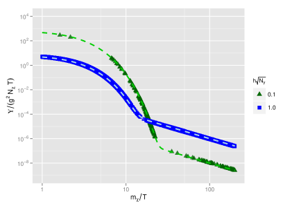
In the low-temperature regime $(T<m_{\chi})$ we are considering here, the pole term in eq. (2.4) dominates for $m_{\chi}/T\sim\mathcal{O}(1)$. In this regime, the sharp peak in on-shell $\chi$ production more than compensates for the Boltzmann suppression, resulting in the enhanced dissipation seen in fig. (1). For $m_{\chi}/T\gtrsim 15$, the exponential suppression of the pole term allows the low-momentum term to dominate once again. The main purpose of this work is to show that the enhancement of dissipation in the pole regime allows for a significant era of warm inflation with smaller $N_{\chi}$ and $g$ than the low-momentum regime.

Figure 1: Full dissipation coefficient as a function of $m_{\chi}/T$ for effective couplings $\hat{h}=h\sqrt{N_{Y}}=\{0.1,1.0\}$. Compare fig. (10) of [23]. The dashed lines represent the numerical prediction made there (cf. their eq. (4.17)). The data points have been obtained from the simulations presented in this work: green triangles stand for points with $h=0.1$, blue squares $h=1$.

3 Observables

For $Q\lesssim 0.1$, quantum and thermal perturbations lead to a perturbation amplitude given by [10, 12]

$$P_{\mathcal{R}}\simeq\left(\frac{H_{\star}}{2\pi}\right)^{\!2}\left(\frac{H_{\star}}{\dot{\phi}_{\star}}\right)^{\!2}\left(1+\frac{T_{\star}}{H_{\star}}\frac{2\pi Q_{\star}}{\sqrt{1+\frac{4\pi}{3}Q_{\star}}}\right)$$ (3.1)

The spectral index is given by

$$n_{\rm s}-1=\frac{\mathrm{d}\ln P_{\mathcal{R}}}{\mathrm{d}\ln k}\simeq\frac{\mathrm{d}\ln P_{\mathcal{R}}}{\mathrm{d}N_{\mathrm{e}}}\,,$$ (3.2)

where $N_{\mathrm{e}}$ is the number of e-folds, and which leads to

$$n_{\rm s}-1 =\frac{\epsilon_{\phi}}{1+Q_{\star}}\left(-6+\frac{3}{2}\frac{\Delta_{\star}}{1+\Delta_{\star}}+\left(2Q_{\star}+A\frac{\Delta_{\star}}{1+\Delta_{\star}}\right)\frac{2+c_{\rm eff}}{4-c_{\rm eff}+Q_{\star}(4+c_{\rm eff})}\right)$$ (3.3)

$$\hphantom{=}+\frac{\eta_{\phi}}{1+Q_{\star}}\left(2-\frac{1}{2}\frac{\Delta_{\star}}{1+\Delta_{\star}}-\left(2Q_{\star}+A\frac{\Delta_{\star}}{1+\Delta_{\star}}\right)\frac{2c_{\rm eff}}{4-c_{\rm eff}+Q_{\star}(4+c_{\rm eff})}\right)$$

$$\hphantom{=}-\frac{\sigma_{\phi}}{1+Q_{\star}}\left(2Q_{\star}+A\frac{\Delta_{\star}}{1+\Delta_{\star}}\right)\frac{4(1-c_{\rm eff})}{4-c_{\rm eff}+Q_{\star}(4+c_{\rm eff})}\,,$$

where all quantities are evaluated at horizon crossing, denoted by a “$\star$”. We have used the slow-roll parameters

$$\epsilon_{\phi}=\frac{m_{\mathrm{P}}^{2}}{2}\left(\frac{V_{\phi}}{V}\right)^{\!2}\,,\qquad\eta_{\phi}=m_{\mathrm{P}}^{2}\frac{V_{\phi\phi}}{V}\,,\qquad\sigma_{\phi}=m_{\mathrm{P}}^{2}\frac{V_{\phi}}{\phi V}\,,$$ (3.4)

and defined

$$c_{\rm eff} =\frac{3{\mathchoice{\mbox{\char 7\relax}}{\mbox{\char 7\relax}}{\mbox{\char 7\relax}}{\mbox{\char 7\relax}}}_{\rm LM}}{{\mathchoice{\mbox{\char 7\relax}}{\mbox{\char 7\relax}}{\mbox{\char 7\relax}}{\mbox{\char 7\relax}}}}+\frac{{\mathchoice{\mbox{\char 7\relax}}{\mbox{\char 7\relax}}{\mbox{\char 7\relax}}{\mbox{\char 7\relax}}}_{\rm pole}}{{\mathchoice{\mbox{\char 7\relax}}{\mbox{\char 7\relax}}{\mbox{\char 7\relax}}{\mbox{\char 7\relax}}}}\left(\frac{1}{2}+\frac{m_{\chi}}{T}\right)\,,$$ (3.5)

$$\Delta_{\star} =\frac{T_{\star}}{H_{\star}}\frac{2\pi Q_{\star}}{\sqrt{1+\frac{4\pi}{3}Q_{\star}}}\,,$$ (3.6)

$$A =\frac{15+Q_{\star}(9+12\pi+4\pi Q_{\star})}{4(3+4\pi Q_{\star})}\,.$$ (3.7)

The above analytical expressions for the amplitude of the spectrum and the spectral index hold only in the weak dissipative regime, $Q_{\star}\lesssim 0.1$. For larger values of the dissipative coefficient, the radiation fluctuations backreact onto the field fluctuations, inducing an enhancement of the spectrum [28, 29, 12] that has to be computed numerically; we are not going to explore that regime in this work. In the limit that dissipation at horizon crossing is dominated by the low-momentum modes, with $c_{\rm eff}\simeq 3$, we recover previous expressions for the spectral index given in the literature [10, 12]. In the limit of very weak dissipation $Q_{\star}\ll 1$ and $\Delta_{\star}\ll 1$, we just recover the standard cold-inflation expression for the spectral index:

$$n_{\rm s}-1\simeq-6\epsilon_{\phi}+2\eta_{\phi}\,.$$ (3.8)

However, this does not mean that predictions are the same as in cold inflation. Even if starting inflation with a small amount of dissipation, the dynamics can increase the value of $Q$, which in turns affects inflaton evolution and therefore the values of the slow-roll parameters. Typically, when $Q$ increases, due to the extra friction added by the dissipation, smaller values of the field are required in order to get $N_{\mathrm{e}}\sim\mathcal{O}(60-50)$.

​​​​​​

​​​​​​

Figure 2: Left: Coefficients of the slow-roll parameters $\epsilon$, $\eta$, and $\sigma$ in the low-momentum limit of equation (3.3) for the spectral index, i.e., $c_{\rm eff}=3$. Right: Same in the pole-dominated regime, ${\mathchoice{\mbox{\char 7\relax}}{\mbox{\char 7\relax}}{\mbox{\char 7\relax}}{\mbox{\char 7\relax}}}\simeq{\mathchoice{\mbox{\char 7\relax}}{\mbox{\char 7\relax}}{\mbox{\char 7\relax}}{\mbox{\char 7\relax}}}_{\rm pole}$, for different values of $m_{\chi}/T$. For small $Q$, the coefficients take their cold-inflation values $\{-6,2,0\}$.

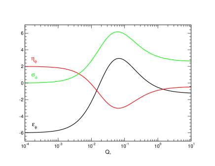
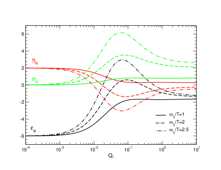
For $Q\gtrsim 10^{-3},$ the form of the spectral index (3.3) changes, with the coefficients now functions of $Q$, as illustrated in fig. (2). In the left panel we have plotted the coefficients for low-momentum-dominated dissipation, while in the right panel we have the pole-dominated case for different values of $m_{\chi}/T=1,\,2,\,2.5$, i.e., different values of $c_{\rm eff}=1.5,\,2.5,\,3$. At large $Q$, the coefficients decrease as $1/Q$.

The coefficients depend also on the combination $Q_{*}(T_{*}/H_{*})$. During slow roll, this quantity can be derived from the radiation equation (2.2) and the perturbation spectrum (3.1)

$$\frac{T_{\star}}{H_{\star}}=\left[\frac{45}{8\pi^{4}}\,\frac{Q_{\star}}{g_{\star}P_{\mathcal{R}}}\!\left(\!1+\frac{T_{\star}}{H_{\star}}\frac{2\pi Q_{\star}}{\sqrt{1+\frac{4\pi}{3}Q_{\star}}}\!\right)\right]^{1/4}\!,$$ (3.9)

Indeed, we can use the Planck observation $P_{\mathcal{R}}=2.2\times 10^{-9}$ to put a first constraint on the amount of dissipation required for warm inflation from eq. (3.9). We conclude that for $g_{\star}=2$ the warm-inflation condition $T>H$ can be satisfied as long as $Q_{\star}>8\times 10^{-8}$, showing that even a very small amount of dissipation can be enough to produce an era of warm inflation.

The primordial tensor perturbation in warm inflation is given by its standard vacuum form:

$$P_{T}=8\left(\frac{H_{\star}}{2\pi m_{\mathrm{P}}}\right)^{2}\,,$$ (3.10)

but the tensor-to-scalar ratio gets modified due to the thermal contribution to the scalar spectrum,

$$r=\frac{16\epsilon_{\star}}{(1+Q_{\star})(1+\Delta_{\star})}\,,$$ (3.11)

where $\epsilon_{\star}=\epsilon_{\phi}/(1+Q)$.

4 Potentials with $\mathbf{m_{\boldsymbol{\chi}}/T=}\text{const.}$

We are mainly interested in exploring the possibility of warm inflation in the pole-dominated regime. Although there is clearly an enhancement of the dissipative coefficient compared to the low-momentum for $m_{\chi}/T\simeq\mathcal{O}(1-10)$, as seen in fig. (1), the dissipative coefficient is suppressed by the Boltzmann factor $\mathrm{e}^{-m_{\chi}/T}$. Whenever the ratio $m_{\chi}/T$ increases during inflation, the pole contribution may quickly vanish, so we first explore which kind of potentials may render this ratio approximately constant during slow-roll inflation.

We derive an equation of motion for $x:=\phi/T$ in warm inflation, starting from

$$\frac{x^{\prime}}{x}=\frac{\phi^{\prime}}{\phi}-\frac{T^{\prime}}{T}=\frac{\phi^{\prime}}{\phi}-\frac{1}{4}\frac{\rho_{\mathrm{R}}^{\prime}}{\rho_{\mathrm{R}}}\,,$$ (4.1)

where a “prime” denotes derivative with respect to the number of e-folds. During slow roll, the energy density in radiation is given by

$$\rho_{\mathrm{R}}=\frac{3}{4}\frac{Q}{(1+Q)^{2}}\frac{V_{\phi}^{2}}{3H^{2}}\,,$$ (4.2)

From this, we obtain

$$\frac{\rho_{\mathrm{R}}^{\prime}}{\rho_{\mathrm{R}}}=\frac{1-Q}{1+Q}\frac{Q^{\prime}}{Q}+2\frac{V_{\phi}^{\prime}}{V_{\phi}}-2\frac{H^{\prime}}{H}\,.$$ (4.3)

From the definition of the dissipative ratio, $Q={\mathchoice{\mbox{\char 7\relax}}{\mbox{\char 7\relax}}{\mbox{\char 7\relax}}{\mbox{\char 7\relax}}}/(3H)$, with Υ given in eq. (2.4), we find

$$\frac{Q^{\prime}}{Q}=-\frac{H^{\prime}}{H}+\frac{\phi^{\prime}}{\phi}-c_{\rm eff}\frac{x^{\prime}}{x}\,.$$ (4.4)

This yields the equation of motion for $x$,

$$\frac{x^{\prime}}{x}=\frac{1}{4-c_{\rm eff}+Q(4+c_{\rm eff})}\left(-\frac{3+Q}{1+Q}\,\epsilon_{\phi}+2\eta_{\phi}-\frac{3+5Q}{1+Q}\,\sigma_{\phi}\right)\,.$$ (4.5)

Hence, we determine potentials that exhibit constant $\phi/T$ by setting $x^{\prime}=0$ and integrating twice the resulting relation between the potential and its derivatives,

$$\frac{V_{\phi\phi}}{V_{\phi}}-\frac{3+Q}{4(1+Q)}\,\frac{V_{\phi}}{V}=\frac{3+5Q}{1+Q}\,\frac{1}{2\phi}\,.$$ (4.6)

For $Q\gg 1$, this yields a potential

$$V^{Q\gg 1}=\mathrm{e}^{C_{1}}\left(C_{2}+\phi^{7/2}\right)^{\!4/3}\,$$ (4.7)

where $C_{1}$ and $C_{2}$ are integration constants. For $Q\ll 1$, we get

$$V^{Q\ll 1}=\mathrm{e}^{C_{1}}\left(C_{2}+\phi^{5/2}\right)^{\!4}\,.$$ (4.8)

Depending on the whether $\phi$ is super- or sub-Planckian, we can write these as either chaotic or hybrid potentials: for $\phi>m_{\mathrm{P}}$,

$$V^{Q\gg 1}\approx V_{0}\left(\frac{\phi}{m_{\mathrm{P}}}\right)^{14/3}\,,\qquad V^{Q\ll 1}\approx V_{0}\left(\frac{\phi}{m_{\mathrm{P}}}\right)^{10}\,,$$ (4.9)

and for $\phi<m_{\mathrm{P}}$,

$$V^{Q\gg 1}\approx V_{0}\left(1+\tilde{\gamma}\left(\frac{\phi}{m_{\mathrm{P}}}\right)^{\!14/3}\right)\,,\qquad V^{Q\ll 1}\approx V_{0}\left(1+\tilde{\gamma}\left(\frac{\phi}{m_{\mathrm{P}}}\right)^{\!10}\right)\,,$$ (4.10)

where we have defined $V_{0}=\lambda m_{\mathrm{P}}^{4}$ for monomial and $V_{0}=\lambda\phi_{\mathrm{c}}^{4}$ for hybrid potentials, $\phi_{\mathrm{c}}$ being the critical field value at which we expect inflation to end via the waterfall transition.

On top of chaotic and hybrid potentials, we will also study hilltop potentials, for different powers of the field. The potentials are then:

Chaotic: $$V=V_{0}\left(\frac{\phi}{m_{\mathrm{P}}}\right)^{p}\,,$$ (4.11)

Hybrid: $$V=V_{0}\left(1+\frac{\gamma}{p}\left(\frac{\phi}{m_{\mathrm{P}}}\right)^{p}\right)\,,$$

Hilltop: $$V=V_{0}\left(1-\frac{\gamma}{p}\left(\frac{\phi}{m_{\mathrm{P}}}\right)^{p}\right)\,.$$

5 Numerical Algorithm

To scan the parameter space of our models for points that allow for a significant amount of warm inflation, we first find initial conditions near a slow-roll trajectory. Once we have identified suitable initial conditions, we check whether they satisfy the necessary constraints for warm inflation. If they do, we let the system evolve until either the slow-roll or the warm-inflation conditions break down or until radiation dominates over the inflaton’s potential energy. The conditions we must verify at each stage for the analytical calculation of the dissipative coefficient eq. (2.4) to hold are: $T\geq H$, $m_{\chi}\geq T$, and the adiabaticity condition on the decay rate of the $\chi$ fields $\Gamma_{\chi}\geq H$.

If $T>H$, we can translate the requirement that the system be in the low-temperature regime, $\frac{m_{\chi}}{T}=\frac{m_{\chi}}{H}\frac{H}{T}>1$, into the necessary (but not sufficient) condition $m_{\chi}/H>1$ or

$$g>\frac{\sqrt{V}}{\phi\,m_{\mathrm{P}}}\,.$$ (5.1)

For the potential $V=\lambda\phi^{4}$ with $\phi\sim\mathcal{O}(1)$ and $\lambda\sim\mathcal{O}(10^{-14}),$ for instance, this translates to $g>10^{-7}$. In fact, we can tighten this constraint by requiring adiabaticity, $\Gamma_{\chi}>H$, which yields

$$g>\frac{64\pi}{h^{2}N_{Y}}\frac{\sqrt{V}}{\phi\,m_{\mathrm{P}}}\,.$$ (5.2)

While small values of $g$ and $h$ favor the pole-dominated regime we are interested in, the above consistency constraints show that the coupling constants cannot be lowered arbitrarily while keeping particle production strong enough for warm inflation and ensuring that the particles produced thermalize quickly.

In order to scan the parameter space, we begin by generating random values for the coupling constants $g$ and $h$, the initial values of $\phi$ and $\rho_{\mathrm{R}}/V_{0}$, the number $N_{\chi}$ of mediator fields, and in the case of hybrid and hilltop potentials, the coupling constant $\gamma$. We then obtain slow-roll initial conditions by simultaneously solving the equation for the Hubble parameter and the slow-roll versions of the equations (2.2) and (2.3) for $V_{0}$, $\dot{\phi}$, and $H$. Hence, the relevant equations are,

$$V_{0} =(3H+{\mathchoice{\mbox{\char 7\relax}}{\mbox{\char 7\relax}}{\mbox{\char 7\relax}}{\mbox{\char 7\relax}}})\,\frac{-\dot{\phi}}{v_{\phi}}\,,$$ (5.3)

$$-\dot{\phi} =\sqrt{\frac{4H\rho_{\mathrm{R}}}{{\mathchoice{\mbox{\char 7\relax}}{\mbox{\char 7\relax}}{\mbox{\char 7\relax}}{\mbox{\char 7\relax}}}}}\,,$$ (5.4)

$$H =\sqrt{\frac{V_{0}v+\rho_{\mathrm{R}}+\frac{1}{2}\dot{\phi}^{2}}{3m_{\mathrm{P}}^{2}}}\,,$$ (5.5)

where we have defined $v=V/V_{0}$. We then use $V_{0}$ to fix one final parameter for each model in order to ensure slow-roll conditions: for monomial and hilltop potentials, we obtain the coupling constant $\lambda$ from $V_{0}=\lambda m_{\mathrm{P}}^{4}$; for hybrid potentials, we set $\lambda=g^{2}$ and use $V_{0}=\lambda\phi_{\mathrm{c}}^{4}$ to fix the critical field value for the waterfall transition in these models.

Given these initial conditions, the system should find itself close to a slow-roll trajectory. We proceed by integrating numerically the full equations of motion for the inflaton, the radiation density, and the scale factor,

$$\frac{\mathrm{d}^{2}\phi}{\mathrm{d}t^{2}} =-\frac{\mathrm{d}V}{\mathrm{d}\phi}-({\mathchoice{\mbox{\char 7\relax}}{\mbox{\char 7\relax}}{\mbox{\char 7\relax}}{\mbox{\char 7\relax}}}+3H)\frac{\mathrm{d}\phi}{\mathrm{d}t}\,,$$ (5.6)

$$\frac{\mathrm{d}\ln\rho_{\mathrm{R}}}{\mathrm{d}t} =\frac{{\mathchoice{\mbox{\char 7\relax}}{\mbox{\char 7\relax}}{\mbox{\char 7\relax}}{\mbox{\char 7\relax}}}}{\rho_{\mathrm{R}}}\left(\frac{\mathrm{d}\phi}{\mathrm{d}t}\right)^{\!2}-4H\,,$$ (5.7)

$$\frac{\mathrm{d}\ln a}{\mathrm{d}t} =H\,.$$ (5.8)

Evolution ends when the slow-roll conditions or the conditions for warm inflation break down. We keep any parameter points that produce at least 1 $\mathrm{e}$-fold of inflation and compare to observational data those that lie between 45 and 55 $\mathrm{e}$-folds.

6 Results

In order to assess the viability of our models, we compare our predictions for the spectral index and the tensor-to-scalar ratio to observations by the Planck satellite [2] in fig. (3). We show the results for chaotic (phi$p$), hilltop (hill$p$), and hybrid (hyb$p$) potentials, for different powers of the field $p$ as indicated in the figure (the label “$4667$” refers to $p=14/3$). For hilltop and hybrid, $p=0$ refers to a logarithmic potential:

$$V=V_{0}\left(1\pm\gamma\ln\left(\frac{\phi}{m_{\mathrm{P}}}\right)\right)\,.$$ (6.1)

For monomial potentials, fig. (4) shows the $n_{\rm s}$–$r$ plane separately with a linear $r$ axis to emphasize the large-$r$ region. We can see that, for increasing $Q$, the trajectory in that plane follows an arc similar to the one seen in refs. [10, 11]. We find low-momentum-dominated points at low $Q$ that allow for a spectral index compatible with Planck results for the $\phi^{4}$ and $\phi^{14/3}$ models; these points do, however, have tensor-to-scalar ratios much bigger than the Planck constraint $r<0.11$. At larger $Q$ and smaller $r$, the trajectory for these two potentials returns to the Planck range for the spectral index; those points tend to be pole-dominated and have $r<10^{-3}$ (compare fig. (3)). We observe further that the maximum $n_{\rm s}$ for each of these models is reached around $Q\approx 5\times 10^{-2}$ and $T/H\approx 50$; this large-$n_{\rm s}$ cusp of the trajectory moves to smaller and smaller $n_{\rm s}$ as the exponent of the potential increases. At its largest values, $n_{\rm s}$ is dominated by the (positive) contributions from the $\eta$ and $\sigma$ terms in expression (3.3); the low-momentum points below $Q\approx 5\times 10^{-3}$ and $T/H\approx 20$, where the coefficients of $\epsilon$ and $\eta$ go through zero, are dominated by the (negative) contribution of the $\epsilon$ term.

For hybrid potentials, our data in both the LM and pole regimes tend to cluster around $n_{\rm s}=1$, with only the quartic hybrid potential producing points compatible with Planck data. The contribution of the $\epsilon$ term to the spectral index tends to be negligible for our hybrid data; instead, $n_{\rm s}$ is set by the (negative) $\eta$ and the (positive) $\sigma$ term.

Quadratic hilltop potentials, however, show points compatible with Planck data in the pole regime. As for the hybrid model, $\epsilon$ at horizon crossing is negligible with respect to $\eta$ and $\sigma$, and therefore the tensor-to-scalar ratio is suppressed and below $r<10^{-3}$.

Figure 3: Tensor-to-scalar ratio $r$ vs spectral index $n_{\rm s}$ for monomial, hilltop, and hybrid potentials. Triangles represent pole-dominated, disks low-momentum-dominated points; color represents the number of mediator fields, $N_{\chi}$. All points lie between 45 and 55 $\mathrm{e}$-folds. The dashed black line and shaded intervals indicate, respectively, the central value and $1\sigma$, $2\sigma$, and $3\sigma$ confidence intervals of $n_{\rm s}$ based on the Planck+lensing data [1].

Figure 4: Tensor-to-scalar ratio $r$ vs spectral index $n_{\rm s}$ for monomial potentials with exponents $p={2,4,\frac{14}{3},10}$. Triangles represent pole-dominated, disks low-momentum-dominated points; color represents the dissipative ratio, $Q$. All points lie between 45 and 55 $\mathrm{e}$-folds. The dashed black line and shaded intervals indicate, respectively, the central value and $1\sigma$, $2\sigma$, and $3\sigma$ confidence intervals of $n_{\rm s}$ based on the Planck+lensing data [1].

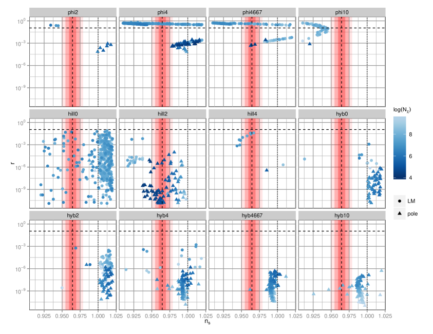
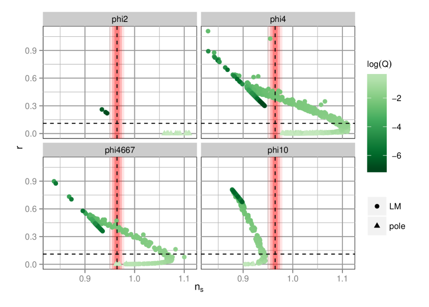
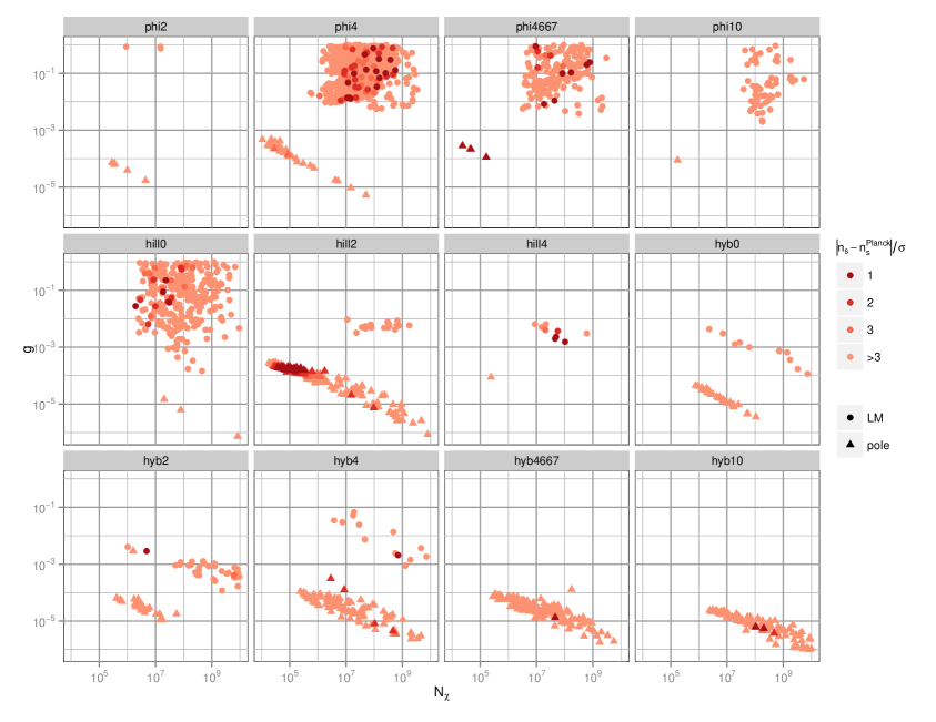
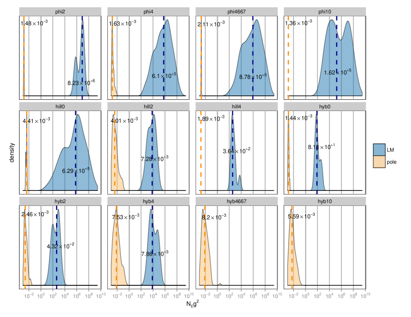
Figure (5) illustrates a main advantage of allowing the pole term to contribute to dissipation: pole-dominated dissipation allows for a significant amount of warm inflation with noticeably smaller values of $g$ and $N_{\chi}$ than the low-momentum regime does. For all potentials, the pole and LM regions are cleanly separated, corresponding to the different ranges of $m_{\chi}/T$ inhabited by the two regimes. The same effect appears in fig. (6), where we compare $N_{\chi}g^{2}$ for low-momentum and pole domination—pole values are consistently smaller. Once we have picked a value for the coupling $g$ that is small enough to keep radiative corrections under control, fig. (6) can provide a rough estimate of the number of mediator fields that need to be introduced to obtain warm inflation.

Figure 5: Points in the $g$–$N_{\chi}$ plane that allow for 45–55 $\mathrm{e}$-folds of inflation. Color indicates the deviation from the central value of $n_{\rm s}$ as measured by Planck+lensing data [1]. Circles indicate low-momentum-dominated dissipation, triangles indicate pole-dominated dissipation.

Figure 6: Distributions and median values of $N_{\chi}g^{2}$ for low-momentum- and pole-dominated points between 45 and 55 $\mathrm{e}$-folds in monomial, hilltop, and hybrid potentials.

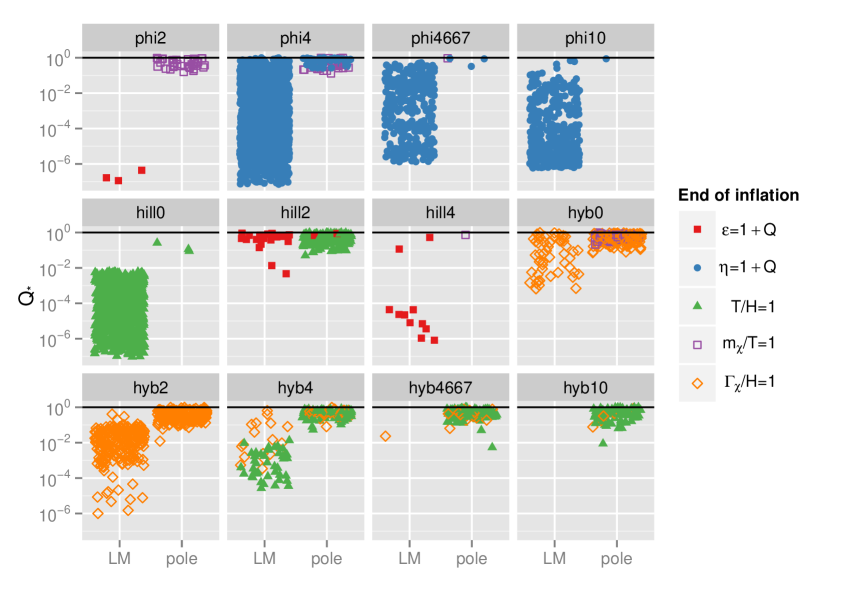
It is interesting to look at the way warm inflation ends; as shown in fig. (7), this stopping condition depends strongly on the potential under consideration. In monomial potentials, we mostly see a breakdown of slow-roll via $\eta=1+Q$; we will take a closer look at these points in section (6.1). For most of our pole points in $\phi^{2}$ and some in $\phi^{4}$ and $\phi^{14/3}$, warm inflation ends with $\Gamma_{\chi}/H=1$.

In the hybrid potentials, $\Gamma_{\chi}/H=1$ is the dominant mode for ending warm inflation, but there remain pole points in the logarithmic and quadratic potentials that end via $m_{\chi}/T=1$; for $p\geq 4$, many points end in $T/H=1$.

Hilltop models, both logarithmic in the LM regime and quadratic in the pole one, have the parameter $T/H$ decreasing by the end of inflation and reaching the lower limit $T/H=1$. For the quadratic model, we have $\eta_{\phi}=\sigma_{\phi}<0$, and therefore from eqs. (A.3) and (A.4) in the weak dissipative regime $Q\ll 1$:

$$\frac{\mathrm{d}\ln T/H}{\mathrm{d}N_{\mathrm{e}}} \simeq-\frac{3-c_{\rm eff}}{4-c_{\rm eff}}\sigma_{\phi}\,,$$ (6.2)

$$\frac{\mathrm{d}\ln\phi/T}{\mathrm{d}N_{\mathrm{e}}} \simeq-\frac{1}{4-c_{\rm eff}}\sigma_{\phi}\,.$$

The ratio $\phi/T$ increases during inflation, and therefore so does $c_{\rm eff}$; when $c_{\rm eff}>4$, the ratio $T/H$ starts to decrease.

It is worth noting that the end of warm inflation does not imply the end of inflation per se. If the temperature drops below the Hubble rate ($T/H<1$) and dissipation is weak ($Q\ll 1$) but slow-roll persists, warm inflation may be followed by an additional phase of cold inflation. We do not investigate that case any further in this work.

Figure 7: Reasons for the end of warm inflation in the pole and LM regimes. For all potentials, the pole regime seems confined to relatively large $Q_{\star}$. All points lie between 45 and 55 $\mathrm{e}$-folds and within $10\sigma$ of Planck’s spectral index.

6.1 Upper bound on $\mathbf{N_{\mathrm{e}}}$ for monomial potentials

The number of $\mathrm{e}$-folds of inflation is given by

$$N_{\mathrm{e}}=\int_{\phi_{\mathrm{i}}}^{\phi_{\mathrm{f}}}\frac{H}{\dot{\phi}}\mathrm{d}\phi=-\int_{\phi_{\mathrm{i}}}^{\phi_{\mathrm{f}}}\frac{V}{V_{\phi}}\frac{1+Q}{m_{\mathrm{P}}^{2}}\mathrm{d}\phi\,.$$ (6.3)

For many of our data points in monomial potentials, inflation ends with $\eta=1+Q_{\mathrm{f}}$ (cf. fig. (7)), which fixes the final field value. If we assume constant $Q=Q_{\mathrm{f}}=Q_{\mathrm{i}},$ we can use the integral (6.3) to set an upper limit on the initial field value for a given number of $\mathrm{e}$-foldings,

$$\phi_{\mathrm{i}}\leq\sqrt{\frac{2pN_{\mathrm{e}}m_{\mathrm{P}}^{2}}{1+Q_{\mathrm{i}}}+\phi_{\mathrm{f}}^{2}}\,.$$ (6.4)

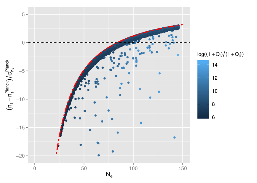
Field values below the upper limit are obtained if $Q$ increases over the course of inflation, which is the case for monomial potentials with exponent $p<14$ in the low-momentum regime [27], and hence for all monomial potentials considered here. Since the slow-roll parameters for monomial potentials are functions of $p$ and $1/\phi^{2}$ only, we can convert this into an upper limit on the low-$Q$ spectral index $n_{\rm s}-1=-6\epsilon+2\eta$,

$$n_{\rm s}-1\leq-\frac{2(p+2)(1+Q_{\mathrm{i}})}{p-1+4N_{\mathrm{e}}}\,.$$ (6.5)

Even for the small values of $Q$ assumed here, dissipation allows $\eta$ to take greater values without slow roll breaking down, and hence the final field value is allowed to be smaller than without dissipation. Additionally, dissipation reduces $\mathrm{d}\phi/\mathrm{d}N_{\mathrm{e}}$, so a smaller field excursion is necessary to produce a given number of $\mathrm{e}$-folds. Dissipation effectively compresses the inflaton field range and shifts it down to lower field values.

For $Q<10^{-6},$ our data show the expected behavior: the spectral index at any given $N_{\mathrm{e}}$ lies below the limit (6.5). For illustration, we include in fig. (8) our low-momentum, low-$Q$ data for the quartic monomial potential alongside the bound (6.5); the width of the densely-populated band below the bound is given by the constraint $Q_{\mathrm{i}}<10^{-6}$ we have imposed on the data in this plot. Scattered below the band are points with large $(1+Q_{\mathrm{f}})/(1+Q_{\mathrm{i}})$, for which $Q$ changes dramatically over the course of inflation and has a significant effect on the integral (6.3) right from the start.

It is interesting to note that, for monomial potentials with exponent $p=\{2,4,\frac{14}{3},10\}$, the low-$Q$ upper limit on $n_{\rm s}$ enters Planck’s $2\sigma$ range at $N_{\mathrm{e}}=\{44,65,73,130\},$ respectively—at least this many $\mathrm{e}$-folds of low-$Q$ warm inflation in the low-momentum regime are necessary for these potentials to produce an observationally-viable spectral index.

For $Q\gtrsim 10^{-3},$ the form of the spectral index (3.3) changes, with the coefficients now functions of $Q$, as illustrated in fig. (2). In this regime, the bound (6.5) no longer applies, and the slow-roll parameters in the spectral index no longer have their simple cold-inflation coefficients. For $Q>10$, these coefficients decrease as $1/Q$ while maintaining fixed ratios ($1:3:-\frac{1}{2}$) between the coefficients of $\epsilon$, $\eta$, and $\sigma$.

Figure 8: Spectral index (in standard deviations from Planck central value) vs $\mathrm{e}$-folds for low-$Q$, low-momentum data in the quartic monomial potential. We have selected points with $Q_{\mathrm{i}}<10^{-6}$, where the spectral index has the form $n_{\rm s}-1=-6\epsilon+2\eta.$ The dot-dashed red line indicates the upper limit (6.5) on $n_{\rm s}$ if dissipation is negligible and inflation ends with $\eta=1+Q$.

7 Conclusions

We have studied warm-inflation dynamics in the low-$T$ regime with a general dissipation coefficient. Dissipation originates from the two-stage mechanism [30, 31], and during inflation a small part of the inflaton energy density is transferred, through a heavy mediator with $m_{\chi}\geq T$, into a thermal bath of light degrees of freedom. In previous analysis, only the low-momentum contribution, from off-shell $\chi$ modes, to the dissipative coefficient was considered when studying the observational implications of warm inflation [27, 32, 33, 10]. In this paper, we have extended the analysis by including on-shell particle production from $\chi$ modes. Although one expects this contribution to be Boltzmann-suppressed for a heavy $\chi$ mode, for sufficiently weak couplings the on-shell contribution can dominate over the low-momentum one [23]. This is due to the different parametric dependence on the Yukawa coupling $h$ of the mediator $\chi$ to the light degrees of freedom. The key point is that the off-shell contribution is proportional to $h$, whilst the on-shell contribution, which peaks near the pole of the $\chi$ spectral density, is inversely proportional to the decay rate of $\chi$ and hence to the coupling $h$.

Typically, dissipation in the low-momentum regime can sustain a sufficiently long period of warm inflation consistent with observations, for instance for the quartic chaotic model. Nevertheless, having enough dissipation requires a large number of mediator $\chi$ fields in the model. We wanted to explore the possibility of reducing this large number of fields by compensating with the enhanced behavior of dissipation in the pole regime. Thus, we have worked with the most general expression for the dissipation Υ in the low-$T$ regime, eq. (2.4), and studied 3 different generic models of single-field inflation: chaotic, hybrid, and hilltop. One might assume that, in order to get large Υ, it is enough to reduce the value of $h$. Consistency of the approximations when computing the dissipative coefficient, however, requires that $\Gamma_{\chi}$, the $T=0$ decay rate of $\chi$ into light degrees of freedom, satisfy the adiabaticity condition $\Gamma_{\chi}>H$; this imposes a lower bound on $h$. This analysis does, however, suggest that if $H$ can be lowered while keeping $\Gamma_{\chi}/h^{2}$ constant or decreasing less, the parameter space of warm-inflation solutions can be extended, a point relevant to consider in future studies.

More generally, this work highlights that, as has been seen in previous warm-inflation model-building work, the need for large field content is not due to the naive expectation that more fields are needed for more dissipation. Instead, it is the complicated set of constraints warm-inflation models have to satisfy that requires a large number of extra fields. The emerging understanding is that only for an appropriate choice of inflaton potentials and underlying field-theory models will we be able to lower the field content. This paper has demonstrated that point and explicitly shown new ways to reduce the field content by looking at the full parametric dependence of the dissipative coefficient alongside the rest of the model.

The main result on the parameters of the model is summarized in fig. (5). The “Low Momentum” and “pole” labels refer to which contribution to Υ dominates at the time of horizon crossing, when the CMB observables are evaluated. There is a clear separation between both regimes depending on the value of the coupling $g$ between the inflaton and the mediator: horizon-crossing pole domination requires small values, $g<10^{-3}$, in order to keep the ratio $m_{\chi}/T\lesssim\mathcal{O}(10)$ and avoid large Boltzmann suppression.

It is also clear from fig. (5) that pole domination allows for smaller numbers of mediator fields than the LM regime. While low-momentum dissipation typically needs a minimum of $\mathcal{O}(10^{6})$ fields in any given model, pole-dominated dissipation in quadratic hilltop models, for example, only requires $\mathcal{O}(10^{4})$ mediators. Such numbers could be achieved in brane-antibrane models of inflation [34]. In fact, it is known that the number of mediators for LM dissipation in brane-antibrane models lies in the range $\mathcal{O}(10^{4}-10^{6})$ [32]; the present analysis shows that that number might drop when we include the pole regime.

The dynamics can make the ratio $m_{\chi}/T$ increase during inflation, such that after pole domination ends, we can continue in the low-momentum regime. Dissipation may even become negligible, allowing inflation to continue some further e-folds in the cold regime; this is an open possibility for the quadratic hilltop model, for example. However, we have not explored those scenarios here, and consider only the regime of warm inflation when deriving the observational constraints. The analysis of the spectrum relies on analytical expressions that hold only in the weak dissipative regime $Q_{\star}<1$, and that is another restriction imposed on the study. While we know from previous studies that there is a growing mode in the LM regime that may lead to too large a tilt in the spectrum [12], such numerical studies have not yet been done for the pole regime. However, for a $T$-dependent dissipative coefficient ${\mathchoice{\mbox{\char 7\relax}}{\mbox{\char 7\relax}}{\mbox{\char 7\relax}}{\mbox{\char 7\relax}}}\propto T^{c}$, we know that the effect is larger the larger the power $c$ [28, 29]. With the general dissipative coefficient, during slow roll it seems that the system behaves like having a dissipative coefficient with ${\mathchoice{\mbox{\char 7\relax}}{\mbox{\char 7\relax}}{\mbox{\char 7\relax}}{\mbox{\char 7\relax}}}\propto T^{c_{\rm eff}}$, where now $c_{\rm eff}$ will change during the evolution. In the pole regime, we have the lower bound $c_{\rm eff}\geq 3/2$, and therefore radiation fluctuations may still influence the spectrum. Nevertheless, although it seems unlikely that the growing mode will disappear completely in the pole regime, its effect can be diminished.

Our aim was to check the possibility of having warm inflation in the pole regime, identify the parameter regions, and study the trend of the observables. It is clear, for example, that the pole regime can give a negligible tensor-to-scalar ratio even for chaotic models. In general, this new regime opens up new possibilities for detailed model building with fewer fields.

Appendix A Slow-roll Equations

In this appendix we give the slow-roll evolution equations for the parameter $Q$ and the ratios $T/H$ and $\phi/T$, in terms of the slow-roll parameters:

$$\epsilon_{\phi}=\frac{m_{\mathrm{P}}^{2}}{2}\left(\frac{V_{\phi}}{V}\right)^{\!2}\,,\qquad\eta_{\phi}=m_{\mathrm{P}}^{2}\frac{V_{\phi\phi}}{V}\,,\qquad\sigma_{\phi}=m_{\mathrm{P}}^{2}\frac{V_{\phi}}{\phi V}\,.$$ (A.1)

They are given by:

$$\frac{\mathrm{d}\ln Q}{\mathrm{d}N_{\mathrm{e}}} \simeq\frac{1}{4-c_{\rm eff}+Q(4+c_{\rm eff})}\left((4+2c_{\rm eff})\epsilon_{\phi}-2c_{\rm eff}\eta_{\phi}-4(1-c_{\rm eff})\sigma_{\phi}\right)\,,$$ (A.2)

$$\frac{\mathrm{d}\ln T/H}{\mathrm{d}N_{\mathrm{e}}} \simeq\frac{1}{4-c_{\rm eff}+Q(4+c_{\rm eff})}\left(\frac{7-c_{\rm eff}+Q(5+c_{\rm eff})}{1+Q}\epsilon_{\phi}-2\eta_{\phi}-(1-c_{\rm eff})\frac{1-Q}{1+Q}\sigma_{\phi}\right)\,.$$ (A.3)

$$\frac{\mathrm{d}\ln\phi/T}{\mathrm{d}N_{\mathrm{e}}} \simeq\frac{1}{4-c_{\rm eff}+Q(4+c_{\rm eff})}\left(-\frac{3+Q}{1+Q}\epsilon_{\phi}+2\eta_{\phi}-\frac{3+5Q}{1+Q}\sigma_{\phi}\right)\,,$$ (A.4)

where:

$$c_{\rm eff}=\frac{3{\mathchoice{\mbox{\char 7\relax}}{\mbox{\char 7\relax}}{\mbox{\char 7\relax}}{\mbox{\char 7\relax}}}_{\rm LM}}{{\mathchoice{\mbox{\char 7\relax}}{\mbox{\char 7\relax}}{\mbox{\char 7\relax}}{\mbox{\char 7\relax}}}}+\frac{{\mathchoice{\mbox{\char 7\relax}}{\mbox{\char 7\relax}}{\mbox{\char 7\relax}}{\mbox{\char 7\relax}}}_{\rm pole}}{{\mathchoice{\mbox{\char 7\relax}}{\mbox{\char 7\relax}}{\mbox{\char 7\relax}}{\mbox{\char 7\relax}}}}\left(\frac{1}{2}+\frac{m_{\chi}}{T}\right)\,.$$ (A.5)

Setting $c_{\rm eff}=3$ in eqs. (A.2)-(A.4), we recover the evolution equations in the low-momentum-dominated regime given in [27].

References

- [1] Planck Collaboration Collaboration, P. Ade et al., Planck 2013 results. XXII. Constraints on inflation, Astron.Astrophys. 571 (2014) A22, [arXiv:1303.5082].
- [2] Planck Collaboration Collaboration, P. Ade et al., Planck 2015 results. XIII. Cosmological parameters, arXiv:1502.01589.
- [3] J. Martin, C. Ringeval, R. Trotta, and V. Vennin, The Best Inflationary Models After Planck, JCAP 1403 (2014) 039, [arXiv:1312.3529].
- [4] S. Tsujikawa, J. Ohashi, S. Kuroyanagi, and A. De Felice, Planck constraints on single-field inflation, Phys. Rev. D88 (2013), no. 2 023529, [arXiv:1305.3044].
- [5] K. Enqvist and M. Karciauskas, Does Planck really rule out monomial inflation?, JCAP 1402 (2014) 034, [arXiv:1312.5944].
- [6] J. Amoros and J. de Haro, The twilight of the single field slow rolling inflaton, arXiv:1503.02153.
- [7] A. O. Barvinsky, A. Yu. Kamenshchik, and A. A. Starobinsky, Inflation scenario via the Standard Model Higgs boson and LHC, JCAP 0811 (2008) 021, [arXiv:0809.2104].
- [8] M. P. Hertzberg, On Inflation with Non-minimal Coupling, JHEP 11 (2010) 023, [arXiv:1002.2995].
- [9] R. Kallosh and A. Linde, Universality Class in Conformal Inflation, JCAP 1307 (2013) 002, [arXiv:1306.5220].
- [10] S. Bartrum, M. Bastero-Gil, A. Berera, R. Cerezo, R. O. Ramos, et al., The importance of being warm (during inflation), Phys.Lett. B732 (2014) 116–121, [arXiv:1307.5868].
- [11] M. Bastero-Gil, A. Berera, R. O. Ramos, and J. G. Rosa, Observational implications of mattergenesis during inflation, JCAP 1410 (2014), no. 10 053, [arXiv:1404.4976].
- [12] M. Bastero-Gil, A. Berera, I. G. Moss, and R. O. Ramos, Cosmological fluctuations of a random field and radiation fluid, JCAP 1405 (2014) 004, [arXiv:1401.1149].
- [13] A. Berera and L.-Z. Fang, Thermally induced density perturbations in the inflation era, Phys. Rev. Lett. 74 (1995) 1912–1915, [astro-ph/9501024].
- [14] A. Berera, Warm inflation, Phys. Rev. Lett. 75 (1995) 3218–3221, [astro-ph/9509049].
- [15] A. Berera, Warm inflation at arbitrary adiabaticity: A Model, an existence proof for inflationary dynamics in quantum field theory, Nucl. Phys. B585 (2000) 666–714, [hep-ph/9904409].
- [16] L. F. Abbott, E. Farhi, and M. B. Wise, Particle Production in the New Inflationary Cosmology, Phys. Lett. B117 (1982) 29.
- [17] A. D. Dolgov and A. D. Linde, Baryon Asymmetry in Inflationary Universe, Phys. Lett. B116 (1982) 329.
- [18] A. Albrecht, P. J. Steinhardt, M. S. Turner, and F. Wilczek, Reheating an Inflationary Universe, Phys. Rev. Lett. 48 (1982) 1437.
- [19] L. Kofman, A. D. Linde, and A. A. Starobinsky, Reheating after inflation, Phys. Rev. Lett. 73 (1994) 3195–3198, [hep-th/9405187].
- [20] J. L. Cook, E. Dimastrogiovanni, D. A. Easson, and L. M. Krauss, Reheating predictions in single field inflation, JCAP 1504 (2015) 047, [arXiv:1502.04673].
- [21] A. Berera, M. Gleiser, and R. O. Ramos, Strong dissipative behavior in quantum field theory, Phys. Rev. D58 (1998) 123508, [hep-ph/9803394].
- [22] M. Bastero-Gil, A. Berera, and R. O. Ramos, Dissipation coefficients from scalar and fermion quantum field interactions, JCAP 1109 (2011) 033, [arXiv:1008.1929].
- [23] M. Bastero-Gil, A. Berera, R. O. Ramos, and J. G. Rosa, General dissipation coefficient in low-temperature warm inflation, JCAP 1301 (2013) 016, [arXiv:1207.0445].
- [24] F. Bezrukov and M. Shaposhnikov, Standard Model Higgs boson mass from inflation: Two loop analysis, JHEP 07 (2009) 089, [arXiv:0904.1537].
- [25] C. Germani and A. Kehagias, New Model of Inflation with Non-minimal Derivative Coupling of Standard Model Higgs Boson to Gravity, Phys. Rev. Lett. 105 (2010) 011302, [arXiv:1003.2635].
- [26] A. A. Starobinsky, A New Type of Isotropic Cosmological Models Without Singularity, Phys. Lett. B91 (1980) 99–102.
- [27] M. Bastero-Gil and A. Berera, Warm inflation model building, Int.J.Mod.Phys. A24 (2009) 2207–2240, [arXiv:0902.0521].
- [28] C. Graham and I. G. Moss, Density fluctuations from warm inflation, JCAP 0907 (2009) 013, [arXiv:0905.3500].
- [29] M. Bastero-Gil, A. Berera, and R. O. Ramos, Shear viscous effects on the primordial power spectrum from warm inflation, JCAP 1107 (2011) 030, [arXiv:1106.0701].
- [30] A. Berera and R. O. Ramos, The Affinity for scalar fields to dissipate, Phys. Rev. D63 (2001) 103509, [hep-ph/0101049].
- [31] I. G. Moss and C. Xiong, Dissipation coefficients for supersymmetric inflatonary models, hep-ph/0603266.
- [32] M. Bastero-Gil, A. Berera, and J. G. Rosa, Warming up brane-antibrane inflation, Phys. Rev. D84 (2011) 103503, [arXiv:1103.5623].
- [33] R. Cerezo and J. G. Rosa, Warm Inflection, JHEP 01 (2013) 024, [arXiv:1210.7975].
- [34] C. P. Burgess, M. Majumdar, D. Nolte, F. Quevedo, G. Rajesh, and R.-J. Zhang, The Inflationary brane anti-brane universe, JHEP 07 (2001) 047, [hep-th/0105204].