A numerical approach for the direct computation of flows including fluid-solid interaction: modeling contact angle, film rupture, and dewetting

Abstract

In this paper, we present a computationally efficient method for including fluid-solid interactions into direct numerical simulations of the Navier–Stokes equations. This method is found to be as powerful as our earlier formulation [J. Comp. Phys., vol. 249: 243 (2015)], while outperforming the earlier method in terms of computational efficiency. The performance and efficacy of the presented method are demonstrated by computing contact angles of droplets at equilibrium. Furthermore, we study the instability of films due to destabilizing fluid-solid interactions, and discuss the influence of contact angle and inertial effects on film breakup. In particular, direct simulation results show an increase in the final characteristic length scales when compared to the predictions of a linear stability analysis, suggesting significant influence of nonlinear effects. Our results also show that emerging length scales differ, depending on a number of physical dimensions considered.

I Introduction

Stability of thin films, in particular at the nanoscale, is relevant in a variety of applications where film breakup and dewetting are important. One example of such applications involves harnessing instabilities of nanoscale liquid metal films in order to create arrays of nanoparticles via self- or directed-assembly kd_pre09 ; fowlkes_nano11 ; Fowlkes2013 ; gonzalez2013 . These methods involve the deposition of thin, solid metal films, that are subsequently exposed to laser pulses; breakup leads to the formation of drops, which then solidify to form nanoparticles. The applications of such nanoparticles are wide, ranging from solar cells to liquid crystal displays, among others fleming_phystoday08 ; maier_natmat03 ; sun_science00 ; maier_2007 ; bader_rmp06 ; min_natmat08 . Such nanofilm breakup presents numerous computational challenges that may result from complex initial geometries Roberts2013 ; Mahadysqw2015 ; however, rupture of a simple flat film due to fluid-solid interactions also demonstrates rich behavior that has been studied extensively in the past (see, for example, sharmaJam1993 ; sharma_jcis99 ; sharma_epje03 , or cm_rmp09 for a review).

To model the film breakup and the consequent dewetting phenomena, it is necessary to include a destabilizing mechanism: if such a mechanism is not included, a continuous film does not break up. In this context, the long-wave formulation (L-W) is usually considered, since it simplifies the underlying mathematical model, reduces dimensionality of the problem, and comes at significantly reduced computational cost. Liquid-solid interaction forces are often included in the L-W as conjoining-disjoining pressure, leading to a prewetted (often called ‘precursor’) layer in nominally ‘dry’ regions. This approach effectively removes the ‘true’ contact line, consequently avoiding the non-integrable shear-stress singularity at the moving contact line (see e.g. Schw98 ; dk_pof07 ; eggers2005 ). Another approach to alleviate the moving contact line singularity is to relax the no-slip condition and instead assume the presence of slip at the liquid-solid interface (see e.g. Hocking2 ; Munch2005 ; afkhami_jcp09 ; Shikhmurzaev ). Slip at the solid surface for fluid-fluid systems has also been studied in the context of molecular dynamics simulations (see e.g. KBW88 ; TR89 ; Thompson1997 ; Ren2007 ). Both slip and disjoining pressure approaches have been extensively used to model a variety of problems including wetting, dewetting, and film breakup, in particular in the context of polymer seeman_prl01 ; becker_nat03 and metal ajaev_pof03 ; trice_prl08 ; kd_pre09 ; fuentes_pre11 ; khenner_pof11 ; Fowlkes2013 ; gonzalez2013 films.

The L-W, however, has its limitations, in particular regarding the requirements of small interfacial slopes and negligible inertial effects. For example, the L-W may not be sufficient to provide quantitatively precise predictions regarding instability development for metal films at nanoscales, where contact angles are large, and inertial effects considerable habenicht_05 ; Habenicht08 ; Fuentes11 ; afkhami-kondic-2013 . Regarding the small slope requirement, it is often argued that the results of the L-W are reasonably accurate even if this requirement is not strictly satisfied; in addition, various improvements of the L-W are available, see, e.g. snoeijer06 . Still, since it is not always possible to compare results of simulations directly to experiments, it is difficult to judge to which degree the L-W based results quantitatively describe the process of thin film breakup. Regarding inertial effects, although the L-W can be extended to include them (see oron_rmp97 ; craster_rmp09 for reviews of this topic), the resulting formulations are not straightforward, and are limited in the range of Reynolds numbers that can be considered.

To be able to accurately model the problems where the assumption of small slopes is not satisfied, or where inertial effects are important, it is necessary to go beyond the L-W, and consider direct solutions of Navier–Stokes equations, that also include fluid-solid interaction forces. It is therefore essential to design a computational method to include the following: (i) precise resolution of long and short range fluid-solid interactions; (ii) allow non-negligible inertial effects and large contact angles; (iii) provide spatially and temporally converged solutions with a reasonable computational cost.

In our earlier work MahadyvdW15 , we developed a model for inclusion of fluid-solid interaction forces in a Navier–Stokes solver. However, that model requires significant computational effort, and it is not practical for use in more complex scenarios, such as three dimensional (3D) film breakup. In the current paper, we present a computational approach that is significantly more efficient. The present approach permits the analysis of complex evolution of the rupturing and dewetting process. Our results reveal that the film initially evolves in accordance to the predictions of the linear stability analysis (LSA) based on the L-W, but departs from the LSA prediction beyond the onset of the instability. We also discuss the influence of the number of physical dimensions considered, by showing differences in the rupture process between two and three dimensions (2D and 3D). Despite the fact that a variety of other computational methods have been considered in the context of wetting/dewetting (see e.g. Jacqmin1999 ; Jacqmin2000 ; Yue2010 ), to our knowledge, the numerical scheme presented in this work provides the only available framework that satisfies all three requirements listed above to quantitatively describe the dynamical evolution of thin film instability including rupture.

This paper is organized as follows. We begin in Sec. II by giving an overview of the computational framework and a brief review of the L-W. We also briefly discuss the LSA of the L-W equations of an initially flat film on a substrate. In Sec. III, we compare the results for the computed contact angle with available results. Then, we present the results of the film instability in linear as well as nonlinear regimes in 2D. We study the underlying physical process, concentrating in particular on the role of the inertia and contact angle to better understand the regimes of the validity of the LSA. Finally, we present simulations of nonlinear evolution and breakup of 3D films and contrast the results with 2D ones. The main conclusions are summarized in Sec. IV.

II Model

II.1 Derivation

We consider a solid phase occupying a half-infinite region $y<0$, above which there is a region occupied by two fluids that we conventionally refer to as a vapor phase (variables subscripted $v$) and a liquid phase (variables subscripted $l$). The words ‘vapor’ and ‘liquid’ are used purely conventionally, and do not necessarily signify anything about the physical properties, except that the two phases may differ in terms of their densities and viscosities.

Each particle of fluid phase $i$ interacts with the solid substrate by means of a Lennard-Jones type potential Israelachvili

$$\phi_{is}=K_{is}^{\ast}\left(\left(\frac{\sigma}{r}\right)^{p}-\left(\frac{\sigma}{r}\right)^{q}\right),$$ (1)

where $r$ is the distance between the two particles, and $K_{is}^{\ast}$ is the scale of the potential, such that Eq. (1) has a minimum $K_{is}^{\ast}/4$ at $r=(p/q)^{1/(p-q)}\sigma$. We can obtain the total potential energy in phase $i$ due to this interaction by the following expression

$$\Phi_{is}=n_{i}\int_{-\infty}^{\infty}\int_{-\infty}^{0}\int_{-\infty}^{\infty}\phi_{is}n_{s}dxdydz,$$ (2)

where $n_{i}$ and $n_{s}$ are the densities of particles in fluid phase $i$ and the solid substrate, respectively. Performing the integration, we obtain

$$\Phi_{is}(y)=\mathcal{K}_{is}\left[\left(\frac{h^{\ast}}{y}\right)^{m}-\left(\frac{h^{\ast}}{y}\right)^{n}\right]=\mathcal{K}_{is}F(y),$$ (3)

where

$$\mathcal{K}_{is}=2\pi n_{i}n_{s}K^{\ast}_{is}\sigma^{3}\left(\frac{\left[(p-2)(p-3)\right]^{q-3}}{\left[(q-2)(q-3)\right]^{p-3}}\right)^{\frac{1}{p-q}},$$ (4)

$$h^{\ast}=\left[\frac{(q-2)(q-3)}{(p-2)(p-3)}\right]^{\frac{1}{p-q}}\sigma;\quad\quad m=p-3,\quad n=q-3.$$ (5)

Equation (3) gives the total potential per unit volume in fluid phase $i$ due to the interaction with the solid substrate. The quantity $h^{\ast}$ is conventionally referred to as the equilibrium film thickness in the literature dk_pof09 ; dk_pof07 , and we will continue using this convention here. The term equilibrium film thickness arises because $h^{\ast}$ is the thickness of a film that represents an energetic minimum due to Eq. (3), and in this model completely wets the surface of the substrate.

We consider the inclusion of the potential in Eq. (3) in the Navier–Stokes equations for two phases. For clarity, we will refer to two phases as the liquid phase (subscript $l$), and the vapor phase (subscript $v$), i.e. $i=l,v$, although the present formulation applies to any two fluids. In order to do this, we introduce a characteristic function $\chi(x,y,z)$, which takes the value of $1$ inside of the liquid phase, and $0$ inside the vapor phase. The interface between these two phases is assumed to be sharp, so that $\chi$ changes discontinuously at the interface. The governing equations consequently become

$$\rho(\chi)\frac{D\textbf{u}}{Dt}=-\nabla p+\nabla\cdot\left[\mu(\chi)\left(\nabla\textbf{u}+\nabla\textbf{u}^{\top}\right)\right]+\gamma\kappa\delta_{s}\textbf{n}-\mathcal{K}(\chi)\nabla F(y),$$ (6)

$$\nabla\cdot\textbf{u}=0.$$ (7)

Here, $\rho$ is the (phase dependent) density, $\mu$ is the viscosity (phase dependent), $p$ is the pressure, and u is the velocity vector. Also, $D/Dt=\partial_{t}+\textbf{u}\cdot\nabla$ is the material derivative. The surface tension is included as a singular body force Brackbill92 . Here $\gamma$ is the coefficient of surface tension, $\kappa$ is the interfacial curvature, $\delta_{s}$ is a delta function centered on the interface, and n is a normal vector for the interface pointing out of the liquid. The quantities depend on $\chi$ via the following

$$\rho =\rho_{l}\chi+\rho_{v}(1-\chi),$$

$$\mu =\mu_{l}\chi+\mu_{v}(1-\chi),$$

$$\mathcal{K} =\mathcal{K}_{ls}\chi+\mathcal{K}_{vs}(1-\chi).$$

In order to nondimensionalize, Eqs. (6) - (7), we introduce the length scale $L$, and define the time scale as the capillary time, $\tau=\mu_{l}L/\gamma$, since, for the parameter sets considered in this paper the dynamics is dominated by viscous and surface tension effects. The dimensionless variables are defined as follows

$$\tilde{x}=\frac{x}{L};\quad\tilde{y}=\frac{y}{L};\quad\tilde{z}=\frac{z}{L};\quad\tilde{t}=\frac{t}{\tau};$$

$$\tilde{h}^{\ast}=\frac{h^{\ast}}{L};\quad\tilde{\textbf{u}}=\frac{\textbf{u}\tau}{L};\quad\tilde{p}=\frac{Lp}{\gamma};\quad\tilde{\kappa}=L\kappa;\quad\tilde{\rho}=\frac{\rho}{\rho_{l}};\quad\tilde{\mu}=\frac{\mu}{\mu_{l}};\quad\tilde{\delta_{s}}=L\delta_{s}.$$

With these scales, and dropping the tildes, the dimensionless Navier–Stokes equations become

$$(\mbox{Oh}^{2})^{-1}\rho\frac{D\textbf{u}}{Dt}=-\nabla p+\nabla\cdot\left[\mu(\nabla\textbf{u}+\nabla\textbf{u}^{T})\right]+\kappa\delta_{s}\textbf{n}-K\nabla F(y),$$ (8)

where the Ohnesorge number is defined via $\mbox{Oh}^{2}=\mu_{l}^{2}/(\rho_{l}\gamma L)$, with $L$ chosen according to the problem under consideration, and

$$K=K_{ls}\chi+K_{vs}(1-\chi)=\frac{\mathcal{K}}{\gamma L^{3}}=\frac{1}{\gamma L^{3}}\left(\mathcal{K}_{ls}\chi+\mathcal{K}_{vs}(1-\chi)\right).$$

Equation (7) is invariant with this scaling. In MahadyvdW15 , we solved Eq. (8) directly. In that paper, we described two methods that we here refer to as ‘body force’ methods; in these methods, we discretized the fluid-solid interaction term differently, but we found both methods to be substantially similar in their overall properties. For consistency, when we refer to the ‘Body Force’ (B–F) method in this paper, we exclusively refer to Method II in MahadyvdW15 . As described in our previous work, the fluid-solid term presents a challenge for body force methods, in that the potential is divergent as $y\rightarrow 0$. Consequently, parts of the domain near the substrate require a high mesh resolution in order to obtain reasonably accurate results. This requirement significantly limits the use of adaptive meshes, that are crucial for the purpose of improving the performance of direct simulations. In 2D, simple problems are feasible, however, in 3D, the computational cost of resolving so much of the domain makes the simulations impractical.

In this section, we show that the computational task is dramatically simplified by reformulating the body force term in Eq. (8) as a force which acts only on the interface. First, we define

$$p^{\ast}=p+K_{ls}\chi F(y)+K_{vs}(1-\chi)F(y),$$

so that

$$-\nabla p^{\ast}=-\nabla p-(K_{ls}\chi+K_{vs}(1-\chi))\nabla F-(K_{vs}-K_{ls})\delta_{s}\textbf{n}F(y),$$

where $\delta_{s}\textbf{n}=-\nabla\chi$, in a distributional sense. Substituting into Eq. (8), we obtain what we refer to as the ‘Reduced Pressure’ (R–P) formulation

$$(\mbox{Oh}^{2})^{-1}\rho\frac{D\textbf{u}}{Dt}=-\nabla p^{\ast}+\nabla\cdot\left[\mu(\nabla\textbf{u}+\nabla\textbf{u}^{T})\right]+(\kappa+\varkappa F(y))\delta_{s}\textbf{n},$$ (9)

where $\varkappa=(K_{vs}-K_{ls})$ (note that only this difference is relevant, rather than individual values of $K_{vs}$ and $K_{ls}$).

Simple energy arguments MahadyvdW15 can be used to show that the fluid-solid interaction term in Eq. (9) gives rise to an equilibrium contact angle $\theta_{\text{eq}}$ for the liquid phase given by

$$\varkappa=\frac{(1-\cos\theta_{\text{eq}})}{h^{\ast}}\left(\frac{(m-1)(n-1)}{m-n}\right).$$ (10)

The exact meaning of $\theta_{\text{eq}}$ requires some clarification. For the fluid-solid interaction considered (with conjoining and disjoining components), there is a film of thickness $h^{\ast}$ that wets the entire substrate, with a smooth transition from the droplet to the equilibrium film. We measure contact angles by fitting a circular profile to the droplet profile ‘away’ from the transition region; the angle at which this circular profile intersects the equilibrium film is taken to be the contact angle. The angle $\theta_{\text{eq}}$ is the equilibrium contact angle in the following sense: for a drop at equilibrium with a vanishingly small $h^{\ast}$, applying the above fitting procedure yields $\theta_{\text{eq}}$. For non-vanishing but small $h^{\ast}$, a drop at equilibrium will have a (slightly) different contact angle, which we refer to as $\theta_{\text{num}}$.

In addition to the contact angle, the fluid-solid interaction gives rise to another phenomenon that we consider in this paper: the spontaneous rupture of a thin liquid film. Our account of film rupture comes from dk_pof07 , where this phenomenon is studied in the context of the L-W. For completeness, in Sec. II.3, we outline the L-W based approach for inclusion of the fluid-solid interaction using the disjoining pressure model.

II.2 Computational Implementation

The R–P method discussed in this paper possesses three important strengths. First, in contrast to conventional methods for implementing the contact angle, that impose it essentially as a constraint that the solution needs to satisfy, it possesses the most important feature of the B–F method discussed in MahadyvdW15 : it includes long range fluid-solid interaction, and therefore spontaneous film breakup can occur. This feature is crucial if one wants to analyze instability of fluid films on nanoscale. The second major advantage of the formulation presented in this work is that by absorbing the entire contribution of the fluid-solid interaction into a surface force, the main weakness of the B–F method is avoided. As discussed previously MahadyvdW15 , the B–F method significantly limits the usefulness of adaptive mesh refinement. Since the force term in the B–F method applies everywhere in the fluid domain, and is singular as $y\rightarrow 0$, the entire domain near $y=0$ requires a finer mesh in order to resolve the force; a typical adaptive mesh for simulations from MahadyvdW15 using the B–F method is shown in Fig. 1(a). In the R–P method, the force due to the fluid-solid interaction is applied as a surface force; consequently, high resolution is only required at the interface. Figure 1(b) shows an adaptive mesh used for simulations using the R–P method in this paper. A further advantage of the R–P method is that it is relatively simple to implement, owing to the fact that it can be formulated as a modification of the curvature in the surface tension term in the Navier–Stokes equations.

We solve Eqs. (9) using the software package Gerris popinetGerris , described in detail in Popinet2009 . The mesh consists of a quad tree (in 2D) or an octree (in 3D), that decomposes the domain into square control volumes, which we refer to as cells (see Fig. 1). We use an adaptive mesh for all simulations, refining the interface to a resolution of $\Delta_{\text{max}}$, and to lower resolutions far away from the interface.

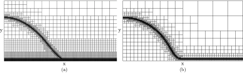
Figure 1: (a) Illustration of a typical adaptive mesh required for the B–F method. The fluid-solid interaction applies everywhere in the domain, requiring increased resolution along the bottom of the domain. (b) Illustration of the adaptive mesh used for simulations reported in this paper. The interface is the only portion of the domain that needs to be resolved at high resolution, due to the fact that the fluid-solid interaction is included as an interfacial force.

The interface is tracked using the Volume of Fluid (VoF) method. The VoF method replaces the characteristic function $\chi$ of Eq. (6) with its average over each cell. This cell average is referred to as the volume fraction, $T$, and denotes the fraction of each computational cell occupied by the liquid phase. The VoF method reconstructs the interface as a sharp interface which is piecewise linear in each cell. Our fluid-solid interaction is included as a modification of the curvature in the surface tension term described in  Popinet2009 . In this method, the curvature, $\kappa$, is calculated at cell centers, and our method replaces it with $\kappa+KF(y)$, where $y$ is the $y$-coordinate of the midpoint of the interface in an interfacial cell. The boundary conditions are as follows: on the solid substrate, we impose no-slip and $T=1$; on all other boundaries, we impose a homogeneous Neumann boundary condition on all variables.

II.3 Long-wave formulation (L-W)

The long-wave formulation (L-W) describes the evolution of the liquid film thickness, $h(x)$ (or $h(x,z)$ in 3D), subject to the well-known assumptions of small interfacial slopes (and therefore small contact angles) and negligible inertial effects see, e.g. oron_rmp97 for an extensive review of the L-W. In the present work, we will use the linear stability analysis (LSA) of the L-W to validate the simulation results and to highlight the differences between the LSA predictions and the direct numerical simulations, in particular in the presence of inertia and large contact angles. We note that the focus in this paper is not on extensive comparison between the simulation and the L-W results. Such a comparison can be found in mahady_13 for spreading and retracting droplets.

In L-W, an additional contribution, of the form $\Pi(h)=\mathcal{K}_{is}F(h)$, to the evolution equation is made to include the fluid-solid interaction. Note that $\Pi(h)$ is of the same form as the fluid-solid interaction term, Eq. (3), formulated for a flat film. See MahadyvdW15 for more details, and oron_rmp97 ; Schwartz-review2002 for reviews; an extensive discussion regarding inclusion of disjoining pressure in the L-W equation can be found in dk_pof07 . With $\Pi(h)$ included, the dimensionless L-W equation is given by

$$3h_{t}+\nabla_{x,z}\cdot(h^{3}\nabla_{x,z}\nabla_{x,z}^{2}h)+\nabla_{x,z}\cdot\left[h^{3}\nabla_{x,z}KF(h)\right]=0,$$ (11)

where $\nabla_{x,z}$ stands for 2D in-plane gradient operator. Equation (11) is derived using the same scales as the ones used to obtain Eq. (8), with the same length scale chosen for both the in–plane directions ($x$ and $z$) and the film thickness ($h$). The LSA of Eq. (11) shows that if the initial film thickness, $h_{0}$, is perturbed by a mode with infinitesimal amplitude, $\delta$, of the form $\exp(i(kx+lz))$, then the initial perturbation will grow or decay with a growth rate

$$\beta=\frac{h_{0}^{3}(k^{2}+l^{2})(k_{c}^{2}-(k^{2}+l^{2}))}{3},$$ (12)

where $k_{c}$ is the critical wavenumber, given by

$$k_{c}^{2}=-\frac{K}{h_{0}}\left[m\left(\frac{h^{\ast}}{h_{0}}\right)^{m}-n\left(\frac{h^{\ast}}{h_{0}}\right)^{n}\right].$$ (13)

Note that if $k_{c}^{2}<0$, then $\beta<0$, and there is no instability for any wavenumber. If $k_{c}^{2}>0$, all modes with wavenumber $k<k_{c}$ are unstable. Associated with Eq. (12) is a wavenumber of maximum growth, $k_{\text{max}}$, and the corresponding maximum growth rate, $\beta_{\text{max}}$, given by

$$k_{\text{max}}=\frac{k_{c}}{\sqrt{2}};\quad\beta_{\text{max}}=\beta(k^{2}+l^{2}=k_{\text{max}}^{2})=\frac{k_{c}^{4}}{12}.$$ (14)

We will frequently make reference to the wavelength of maximum growth, defined by $\lambda_{\text{max}}=2\pi/k_{\text{max}}$.

Within the L-W, these results imply the following features of the film instability:

• The wavenumber of maximum growth, $k_{\text{max}}$, scales with $\sqrt{1-\cos\theta_{\text{eq}}}$. Large contact angles imply larger $k_{\text{max}}$, and a corresponding decrease in $\lambda_{\text{max}}$.

• The maximum growth rate, $\beta_{\text{max}}$, scales with $(1-\cos\theta_{\text{eq}})^{2}$. Large contact angles dramatically increase the growth rate of the dominant mode, and thus reduce the time it takes for films to break up.

III Results

III.1 Contact Angles

We first demonstrate that the method under consideration can yield contact angles as accurately as the methods presented in MahadyvdW15 . For this purpose, we consider a 2D droplet, with the initial fraction (the initial region occupied by the liquid phase, i.e. where $T=1$) set to be the following

$$\{(x,y):x^{2}+(y+R\cos\theta_{i}-h^{\ast})^{2}<R^{2}\text{ or }y<h^{\ast}\}.$$

Thus the initial profile is a circular cap sitting on top of an equilibrium film such that it intersects this film with angle $\theta_{i}$. The value of $R$ is chosen so that the total area of the circular cap is equal to $A_{0}=0.75^{2}\pi/2$. For simplicity, for our first tests, we set $\theta_{\text{eq}}=\theta_{i}=\pi/2$. Since for small $h^{\ast}$, $\theta_{\text{num}}$ is close to $\theta_{\text{eq}}$, the initial fluid configuration is close to its equilibrium. The droplet is then allowed to relax, and we measure $\theta_{\text{num}}$ via the method described in Sec. II. We set $\mbox{Oh}=(0.05)^{-1/2}$, a sufficiently large value so that inertial effects are not significant.

$\Delta$	R–P	B–F
$1/2^{5}$	$6.1\times 10^{-2}$	$7.0\times 10^{-3}$
$1/2^{6}$	$2.6\times 10^{-3}$	$4.3\times 10^{-3}$
$1/2^{7}$	$8.0\times 10^{-4}$	$3.8\times 10^{-4}$

Table I: Comparison of the mesh convergence between the R–P method and the B–F method of MahadyvdW15 for a drop. Here, $\Delta$ is the grid resolution used (the maximum one for the R–P method, and uniform for the B–F method), and the L¹ norm of the error in the profile shape. The performance of the two methods is comparable at higher resolutions.

Table I compares the convergence of the equilibrium droplet profile as a function of the minimum mesh size, for a droplet simulated using the R–P method discussed here, and the B–F method of MahadyvdW15 . The R–P simulations are resolved to a resolution $\Delta_{\text{max}}=\Delta$ on an adaptive mesh as shown in Fig. 1, while the B–F method simulations are refined uniformly with mesh size $\Delta$. The error is measured as the L¹ norm of the error in the profile shape. The equilibrium film thickness is $h^{\ast}=0.03$. Despite the fact that the B–F simulations are run with a uniform mesh, the R–P method performs comparably well in convergence in mesh to the B–F method at higher resolutions.

Figure 2 shows simulation profiles obtained using the R–P method, again with $\theta_{\text{eq}}=\theta_{i}=\pi/2$. The profiles at equilibrium are shown for $h^{\ast}=0.03$ (red) , $h^{\ast}=0.015$ (green), and $h^{\ast}=0.0075$ (blue). The initial condition for $h^{\ast}=0.015$ is plotted by the black dotted line, showing the profile of a droplet with contact angle $\theta_{\text{eq}}$. The smooth transition from the droplet profile to the equilibrium film is clearly visible; as $h^{\ast}$ is reduced, the equilibrium profiles approach those of a droplet with contact angle $\theta_{\text{eq}}$.

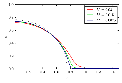
Figure 2: Effect of $h^{\ast}$ on the profile when $\theta_{i}=\theta_{\text{eq}}=\pi/2$. The dotted line shows the initial profile for $h^{\ast}=0.015$.

$h^{\ast}$	R–P	B–F
0.03	1.36	1.37
0.015	1.45	1.47
0.0075	1.49	1.53

Table II: The contact angle, $\theta_{\text{num}}$, obtained by the R–P and the B–F methods for different values of $h^{\ast}$. The contact angles approach $\theta_{\text{eq}}=\pi/2$ at a similar rate.

Table II shows the measured values of $\theta_{\text{num}}$, again for the droplet with $\theta_{\text{eq}}=\theta_{i}=\pi/2$, as $h^{\ast}$ is varied, for both the B–F and the R–P methods. While the values differ slightly between the two methods, as $h^{\ast}$ is reduced, $\theta_{\text{num}}$ becomes closer to $\theta_{\text{eq}}$.

We conclude that the R–P method is comparable to the B–F method in its ability to model the contact angle. In addition, it comes with the potential for dramatically improved performance, due to fact that the layer of fluid near the substrate does not necessarily need to be highly resolved. For example, for the drops simulated in Table I, with the timestep fixed at $10^{-5}$, at $\Delta=1/2^{6}$ the R–P method takes approximately $14\%$ as much CPU time as the B–F method; at $\Delta=1/2^{7}$, the R–P method has approximately $5\%$ the runtime. This is because, for each timestep, the number of computations each method incurs is $O(N)$, where $N$ is the number of cells. However, the adaptive mesh illustrated in Fig. 1 has approximately $O(1/\Delta)$ cells, while a uniform mesh has $O(1/\Delta^{2})$ cells. Simple adaptive meshes were used in MahadyvdW15 , improving the performance of the B–F method, however, higher resolution is still required at a layer of nonzero thickness near the substrate. The complexity difference is similar in 3D, where the R–P method scales as $O(1/\Delta^{2})$ and the B–F method as $O(1/\Delta^{3})$.

The improvement in performance permits the study of problems that are impractical to consider using the B–F method, including breakup of the films in 2D and 3D. We proceed to analyze these problems.

III.2 Film Instability: Linear regime

In this section, we compare the LSA predictions of the L-W equation with the results of simulations, both applied to the instability of thin films in 2D. We focus here on early times/linear regime for which the LSA is expected to hold and discuss the comparison between the results influenced by the relevant parameters. In particular we focus on the influence of the unperturbed film thickness, $h_{0}$, and of the equilibrium contact angle, $\theta_{\text{eq}}$. Note that the LSA should apply even for large contact angles, since we focus on early stages of instability when the interfacial slopes are small. We set $\mbox{Oh}=0.45$, which implies a low inertia regime, so that the assumptions of the L-W are reasonably well satisfied (in Sec. III.3, we discuss the values of Oh that constitute low inertia in the present context). For all the simulations, the initial region occupied by the liquid phase (i.e., $T=1$) is between $y=0$ and $h=h(t=0,x)=h_{0}(1+\delta\cos(kx))$, where $\delta=0.08$. For all simulations in this section, we set $h^{\ast}=0.12$.

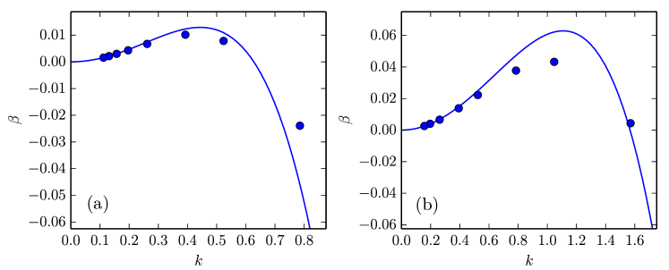
Figure 3: Comparison between the dispersion curve predicted by the LSA of the L-W equation (blue solid curve) and the growth rate computed by R–P based simulations (symbols), for $\theta_{\text{eq}}=\pi/2$, for (a) $h_{0}=1.0$ and (b) $h_{0}=0.5$.

Figure 3 shows the growth rates resulting from the LSA together with the ones extracted from simulations for early time evolution, for a discrete set of wavenumbers. We measure the growth rate of simulations according to the following procedure: first, we output the minimum $y$-coordinate of the fluid interface, $h_{min}(t)$. We then find $t_{0}$ and $t_{1}$, such that for $t_{0}<t<t_{1}$, the function $\log(h_{min}(t))$ is approximately linear in $t$; $t_{0}$ is generally near $0$, and $t_{1}$ is small, so this corresponds to the interval of time when the growth of the unstable modes is governed by the LSA. We then perform a least-squares fit of a line to $\log(h_{min}(t))$ over this interval. Repeating the same procedure for the maximum $y$-coordinate of the fluid interface, $h_{max}(t)$, we calculate the growth rate as the average of the slopes of the fitted lines.

We focus on the influence of $h_{0}$, and set $\theta_{\text{eq}}={\pi/2}$. For small wavenumbers, $k$, the agreement is very good; however, for larger values of $k$, there are significant differences, for both values of $h_{0}$. We conjecture that the differences are due to the fact that the L-W assumptions no longer hold for larger values of $k$, since the separation of scales required for the L-W to apply may not be satisfied. For example, if one considers the relevant lengthscales as $x_{c}=\lambda_{\text{max}}$ and $h_{c}=h_{0}$, in the in-plane and out-of-the-plane direction, respectively, then for $h_{0}=0.5$ one finds $\epsilon=x_{c}/h_{c}$ is $O(0.1)$ and therefore for $k$ values larger than $k_{\text{max}}$, the requirement $\epsilon\ll 1$ is no longer a good approximation. However, it should be noted that the differences between the simulations and the LSA are mostly focused on large values of $k$, where films are stable.

One may expect that the LSA would lead to more accurate results for thinner films. As we can see in Fig. 3, this is not the case. An insight can be reached again by considering the relevant length scales; the ratio of the film thickness, $h_{0}$, and the relevant in-plane length scale, $\lambda_{\text{max}}$, given by

$$\frac{h_{c}}{\lambda_{\text{max}}}=\frac{1}{2\pi}\sqrt{-Kh_{0}\left[m\left(\frac{h^{\ast}}{h_{0}}\right)^{m}-n\left(\frac{h^{\ast}}{h_{0}}\right)^{n}\right]}.$$ (15)

This ratio is a decreasing function of $h_{0}$ for $h_{0}>h^{\ast}\left[m(m-1)/(n(n-1))\right]^{m-n}.$ Therefore, reducing $h_{0}$ actually implies that the LSA is less accurate, except when $h_{0}$ is nearly as small as $h^{\ast}$.

Figure 4: Comparison between the growth rate predicted by the LSA (blue solid curve), and the simulations (symbols), for $h_{0}=0.5$, for (a) $\theta_{\text{eq}}=3\pi/4$, (b) $\theta_{\text{eq}}=\pi/2$, and (c) $\theta_{\text{eq}}=\pi/6$. The value of $k_{\text{max}}$ obtained from simulations is shown by the vertical solid line; the dash-dotted line shows the value of $k_{\text{max}}$ predicted by the LSA.

Equation (15) implies that a reduction in $\theta_{\text{eq}}$ should improve agreement with the predictions of the LSA. Figure 4 shows the results for three values of $\theta_{\text{eq}}$ and we indeed immediately observe much smaller differences between the simulations and the LSA for smaller $\theta_{\text{eq}}$. For larger $\theta_{\text{eq}}$, the LSA strongly overpredicts the growth rates as well as the values of $k_{\text{max}}$. We will see in the next section that the differences between the values of $k_{\text{max}}$ resulting from the simulations and the LSA become much more visible in the nonlinear regime of instability development.

III.3 Film instability: Nonlinear evolution and breakup - 2D

Here we focus on the nonlinear process of film breakup, and concentrate in particular on the role of the contact angle, $\theta_{\text{eq}}$, and Ohnesorge number, Oh, on the properties of emerging patterns. While the discussion that follows is general, and is formulated in terms of previously defined nondimensional quantities, in order to choose a reference parameter set, we consider nanoscale liquid metallic films. The stability properties of such films have been a subject of recent interest in connection with nanoparticle fabrication (see e.g. ajaev_pof03 ; trice_prl08 ; kd_pre09 ; fuentes_pre11 ; khenner_pof11 ; Fowlkes2013 ). In experiments, a film of metal, with thickness on the order of tens of nanometers, is deposited on a surface. This film is then liquefied, and subsequently breaks up into droplets, which solidify to form nanoparticles.

For definitiveness, we focus on Cu films, as considered in gonzalez2013 . The viscosity, density, and surface tension are taken to be the values of liquid Cu at its melting point gonzalez2013 , with $\rho=7760$ kg/m³, $\mu=0.00438$ Pa$\cdot$s, and $\gamma=1.304$ N/m. We set relevant length scale, $L$, as the reference film thickness, taken to be $8$ nm. The Ohnesorge number corresponding to these parameters is $\mbox{Oh}=0.487$. Note that this represents a rough lower bound for Oh in the motivating experiments: temperatures may exceed the melting point substantially, reducing the viscosity, and furthermore the relevant length scales may be larger than $8$ nm. This variation in Oh makes it important to explore the boundary between the viscous and inertial regimes. The simulations that we present in this section are for a film of thickness $h_{0}=1$; we also considered films with $h_{0}=0.5$, and obtained similar results. We use $h^{\ast}=0.1225$, and $\theta_{\text{eq}}=79^{\circ}\approx 0.439\pi$. Note that for these parameters, $\lambda_{\text{max}}=15.6$, and $\lambda_{c}=11.0$.

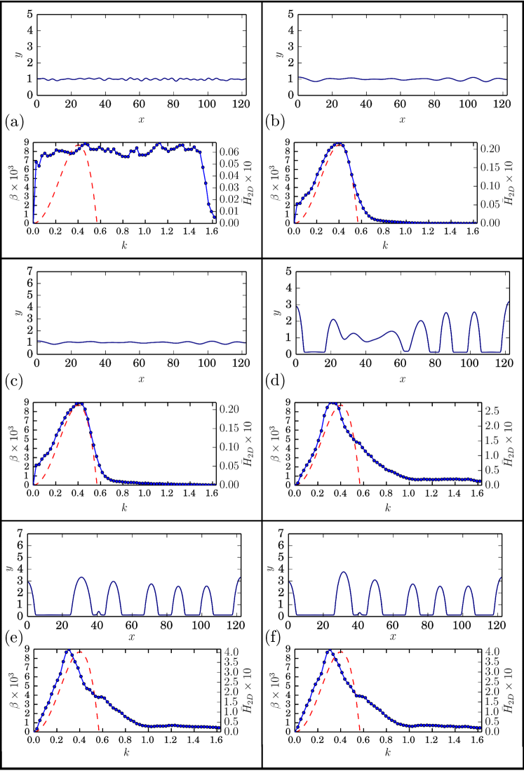
Figure 5: Time evolution of a representative simulation of film breakup in 2D with $h_{0}=1$, $\mbox{Oh}=0.487$, and $\theta_{\text{eq}}=0.439\pi$; the solid blue curve shows the fluid interface. The associated Fourier spectrum, averaged over 20 realizations, is shown below each image. (a) $t=0$, (b) $t=179$, (c) $t=357$, (d) $t=536$, (e) $t=715$, and (f) $t=882$.

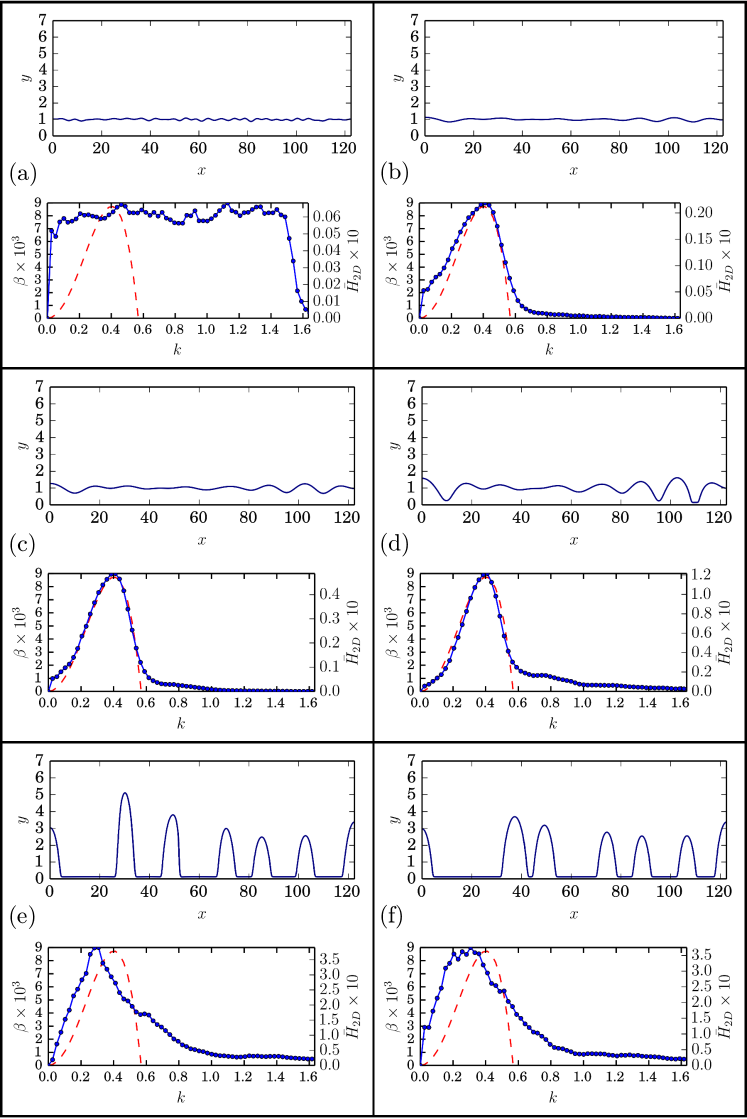
Figure 6: Time evolution of a representative simulation of film breakup in 2D with $h_{0}=1$, $\mbox{Oh}=0.0487$, and $\theta_{\text{eq}}=0.439\pi$; the solid blue curve shows the fluid interface. The associated Fourier spectrum, averaged over 20 realizations, is shown below each image. (a) $t=0$, (b) $t=357$, (c) $t=536$, (d) $t=715$, (e) $t=1429$, and (f) $t=2858$.

For 2D simulations, the computational domain is specified by $(L_{x},L_{y})$, with $L_{x}\approx 8\lambda_{\text{max}}$, and $L_{y}$ sufficiently large so that the value assigned to it does not influence the results. For the simulations discussed next, we use $L_{x}=122.5$, $L_{y}=43.125$, and the initial film shape specified by is $h_{0}+\zeta(x)$, where

$$\zeta(x)=\sum_{i=1}^{60}\delta_{i}\cos\left(\frac{2\pi x}{\lambda_{i}}\right).$$ (16)

Here, $\lambda_{i}=2L_{x}/i$, and $\delta_{i}$ is a random perturbation amplitude, uniformly distributed in the range $\pm 0.0125$. We simulate the evolution with $N_{s}=20$ sets of $\delta_{i}$. For each simulation (numbered $j$), a discrete height profile is produced, $\hat{h}_{j}(t,x)$. We then compute the discrete Fourier transform (DFT) of each height profile, $\hat{H}_{j}(t,k)$. Finally, we compute the average of these as

$$\bar{H}_{2D}(t,k)=\frac{1}{N_{s}}\sum_{j=1}^{N_{s}}\hat{H}_{j}(t,k).$$ (17)

Figure 5 shows the time evolution of a typical profile $\hat{h}_{1}(t,x)$ (the top image in each of Fig. 5(a) - (f)), $\bar{H}_{2D}(t,k)$ along with the dispersion curve from the LSA (the bottom image in each of Fig. 5(a) - (f), smoothed with a running $5$ point average). We see that as the initial perturbations begin to grow, the $\bar{H}_{2D}(t,k)$ attains the form similar to the dispersion curve (Fig. 5(a) -  (c)). However, as the holes and consequently drops start to form, the peak in $\bar{H}_{2D}(t,k)$ shifts towards smaller values of $k$, so that the final distribution of drops is characterized by a length scale larger than $\lambda_{\text{max}}$. Next we consider different values of Oh. For $\mbox{Oh}=4.87$, no significant difference is observed compared to $\mbox{Oh}=0.487$, indicating that both sets of results belong to the high viscosity limit. Smaller values of Oh, however, lead to different results. Figure 6 shows profiles and associated averaged Fourier spectra for a film with $\mbox{Oh}=0.0487$. We see that the film takes much longer to break up compared to the films characterized by larger Oh. Also, the long term evolution of the Fourier spectrum shows a flatter peak, when compared with the larger Oh simulations, indicating that the preference for a specific wavenumber is weaker in the late stages of evolution. The practical consequence of this may be increased degree of disorder in the distribution of emerging patterns.

In order to study the effect of Oh on the evolution of the film more systematically, we define $k^{\text{num}}_{\text{max}}(t)$ as the value of $k$ for which $\bar{H}_{2D}(t)$ attains its maximum. Figure 7 plots $k^{\text{num}}_{\text{max}}$ for various Oh as a function of time (note that due to the finite domain size, $k_{\text{max}}^{\text{num}}$ only takes discrete values, leading to the staircase appearance of these plots). The symbols on each curve indicate the approximate time at which the film ruptures, and the dashed line shows the value of $k_{\text{max}}$ from the LSA.

Figure 7: Comparison of $k_{\text{max}}^{\text{num}}$ as a function of time for films of varying Oh. Symbols show the approximate breakup times for each parameter set, and the solid dashed line shows $k_{\text{max}}$ predicted by the LSA. Note that $\mbox{Oh}=4.87$ and $\mbox{Oh}=0.487$ are visually nearly indistinguishable. The ticks on the $y$-axis are for wavenumbers that can be resolved on the finite domain. Here, $h_{0}=1$, $\theta_{\text{eq}}=0.439\pi$.

The overall behavior is similar for all curves: $k_{\text{max}}^{\text{num}}$ quickly takes a value as close to the $k_{\text{max}}$ as can be resolved on a finite domain, and then stays at this value until the film breaks up. Afterwards, it decreases, indicating that the length scale of the final droplet distribution is larger than $\lambda_{\text{max}}$. We note that for $\mbox{Oh}=4.87$ and $\mbox{Oh}=0.487$, the behavior is nearly indistinguishable, indicating large Oh limit. Most importantly, smaller values of Oh significantly increase the time it takes for the film to rupture. The LSA does not capture this behavior, and instead predicts that the breakup time is approximately the same ($\approx 500$) for all values of Oh, consistently with the results of large Oh simulations.

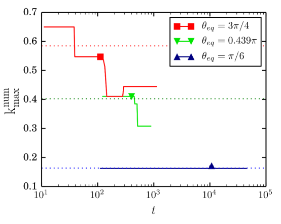
Figure 8: Plot of $k_{\text{max}}^{\text{num}}$ for varying $\theta_{\text{eq}}$. The green curve corresponds to $\mbox{Oh}=0.487$ in Fig. 7. The symbols show the approximate time of film rupture. Each dashed line shows $k_{\text{max}}$ from the LSA for the curve of the same color.

Next, we investigate the effect of the contact angle on the rupture. We carry out two additional simulation sets, both with $\mbox{Oh}=0.487$, and with different values of $\theta_{\text{eq}}$ and different domain sizes, keeping $L_{x}\approx 8\lambda_{\text{max}}$:

1. $\theta_{\text{eq}}=\pi/6$, $L_{x}=367.5$;

2. $\theta_{\text{eq}}=3\pi/4$, $L_{x}=91.875$.

For each set, the form of the perturbation is the same as in Eq. (16), using corresponding values of $L_{x}$. Figure 8 shows $k_{\text{max}}^{\text{num}}$ for these two contact angles, as well as for $\theta_{\text{eq}}=0.439\pi$. For each curve, the symbol of the same color indicates the breakup time, and the dashed line of the same color shows $k_{\text{max}}$ from the LSA. Note that the breakup times predicted by the LSA are $\approx 18000$, $500$, and $110$, for $\theta_{\text{eq}}=\pi/6$, $0.439\pi$, and $3\pi/4$, respectively, roughly in line with the simulated breakup time for all cases. For $\theta_{\text{eq}}=3\pi/4$, the behavior is similar to $\theta_{\text{eq}}=0.439\pi$. However, the evolution of $\theta_{\text{eq}}=\pi/6$ is dramatically simpler: almost immediately, $k_{\text{max}}^{\text{num}}$ relaxes to near $k_{\text{max}}$, and remains at approximately the same value for the considered simulation times.

To gain a basic understanding of the influence of $\theta_{\text{eq}}$ on the evolution, consider the following simple argument. Approximate the profile of a rupturing film of unit initial thickness, perturbed by a mode of wavelength $\lambda_{\text{max}}$, by $h(x)=1+A(t)\cos\left(2\pi x/\lambda_{\text{max}}\right),$ where $A(t)$ is the time dependent amplitude. At the time of breakup, $A\approx 1$. Then, further approximate the instantaneous contact angle, $\theta_{r}$, of the rupturing film by considering the slope at the point of inflection, given by $\tan\theta_{r}=2\pi/\lambda_{\text{max}}$. Substituting the value of $\lambda_{\text{max}}$, we obtain $\tan\theta_{r}=B\sqrt{1-\cos\theta_{\text{eq}}},$ with $B=\sqrt{-\left(m{h^{\ast}}^{m}-n{h^{\ast}}^{n}\right)2\sqrt{2}h^{\ast}}.$ Consider now the difference between $\theta_{r}$ and $\theta_{\text{eq}}$. This difference is an increasing function of $\theta_{\text{eq}}$, suggesting that when films with larger $\theta_{\text{eq}}$ rupture, the corresponding $\theta_{r}$ is significantly different from $\theta_{\text{eq}}$, leading to quick retraction of the film from the point of rupture. This retraction reduces the space available for consecutive breakups, and leads to larger distances between the drops than predicted by the LSA. For smaller values of $\theta_{\text{eq}}$, the difference between $\theta_{r}$ and $\theta_{\text{eq}}$ is small at the point of initial rupture, and the retraction effect is not present.

Next we comment on the difference between $k_{max}^{num}$ and the corresponding $k_{max}$, visible in Figs. 7 - 8. First we note that this shift is not affected by inertial effects for the simulated times: Fig. 7 shows that $\mbox{Oh}=48.7$ and $\mbox{Oh}=0.0487$ lead to the same $k_{max}^{num}$ after breakup (the additional coarsening expected for very long times is beyond the scope of the present study). These results cannot be explained by the breakdown of the LSA for large $\theta_{eq}$: from Fig. 4, we might expect a roughly 10% difference between the wavelength of maximum growth in LSA and simulations, which is significantly less than the difference between $k_{max}^{num}$ and $k_{max}$ after the film has ruptured. Thus, we expect that the difference is due to nonlinear effects relevant during breakup for larger contact angles. We note here that for for smaller contact angles the effect is not visible within the present degree of accuracy; the simulations carried out in larger domains and with larger number of realizations using long-wave approach suggest that (much less obvious) coarsening effects may be seen within long-wave simulations as well nesic_15a .

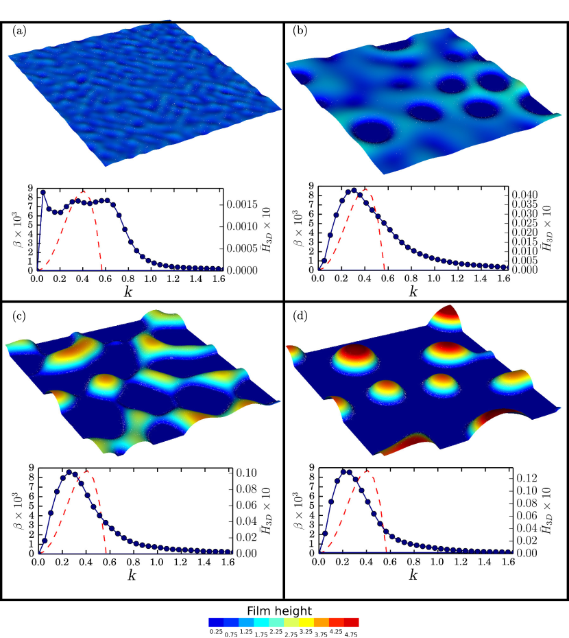
Figure 9: Time evolution of a representative simulation of film breakup in 3D, with $\mbox{Oh}=0.487$, $h_{0}=1.0$, and $\theta_{\text{eq}}=0.439\pi$. The color shows the logarithm of the height of the interface above the substrate. The associated Fourier spectrum is shown below each image; these data are averaged over 10 instances, and smoothed with a 5 point running average. (a) $t=0.0$, (b) $t=335$, (c) $t=558$, and (d) $t=781$.

III.4 Film instability: Nonlinear evolution and breakup - 3D

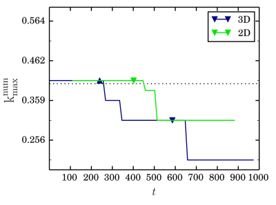
Figure 10: Comparison of $k_{\text{max}}^{\text{num}}$ as a function of time for 3D films (blue) and 2D films (green). The green inverted triangle shows the approximate breakup time of the 2D simulation. The blue triangle shows the approximate time at which the first holes form in the 3D film; the inverted blue triangle shows the approximate time that droplets begin to form. The solid dashed line shows $k_{\text{max}}$ predicted by the LSA.

Next, we consider film breakup in 3D. The setup is identical to the 2D case, except that the domain size is specified by $L_{x}=L_{z}=4\lambda_{\text{max}}$ and $L_{y}=31.25$. The initial condition is a perturbed film specified by $h_{0}+\zeta(x,z)$, and

$$\zeta(x,y)=\sum_{i=1}^{30}\sum_{j=1}^{30}\delta_{ij}\cos\left(\frac{2\pi x}{\lambda_{i}}\right)\cos\left(\frac{2\pi z}{\lambda_{j}}\right),$$ (18)

where $\lambda_{i}=2L_{x}/i$, and $\delta_{ij}$ are random perturbation amplitudes, uniformly distributed in the range $\pm 0.0125$. We simulate the film for $N_{s}=10$ sets of $\delta_{ij}$. As in the 2D case, we produce a height profile for each simulation, $\hat{h}_{j}(t,x,z)$, compute its discrete Fourier transform, $\hat{H}_{j}(t,k,l)$, and the average

$$\bar{H}_{3D}(t,k)=\frac{1}{N_{s}}\sum_{j=1}^{N_{s}}\frac{1}{2}\left(\hat{H}_{j}(t,k,0)+\hat{H}_{j}(t,0,k)\right).$$ (19)

The summand in Eq. (19) represents the average of the discrete Fourier transforms along the coordinate axes, taking advantage of the symmetry of Eq. (12) to get more information about the growth rates.

Figure 9 shows the time evolution of $\hat{h}_{1}(t,x,z)$ (top image in each part of the figure), and $\bar{H}_{3D}$ along with the dispersion curve predicted by Eq. (12) (bottom images). The plots of $\bar{H}_{3D}$ have been smoothed by a $5$ point running average. A similar trend is observed as in Fig. 5: the spectrum takes on a similar profile to the dispersion curve from the LSA, and as breakup proceeds, its peak, $k_{\text{max}}^{\text{num}}$, shifts towards smaller wavenumbers.

Figure 10 shows $k_{\text{max}}^{\text{num}}(t)$ for both 2D and 3D films ($\mbox{Oh}=4.87$). For both 2D and 3D, $k_{\text{max}}^{\text{num}}$ is close to $k_{\text{max}}$ until the film ruptures, after which both $k_{\text{max}}^{\text{num}}$ relax to smaller values. However, once droplets begin to form in 3D simulations, $k_{\text{max}}^{\text{num}}$ relaxes to an even smaller value. The same retraction argument that we used to explain the evolution of $k_{\text{max}}^{\text{num}}(t)$ in 2D can as well be used here to explain this phenomenon.

We also study the effect of initial film thickness on the evolution of the Fourier spectra for 3D films. Figure 11 presents the evolution of the film with an initial thickness $h_{0}=0.5$, while keeping $\theta_{eq}$, $h^{\ast}$, and Oh the same as in Fig. 9. Our initial condition is again subject to a white noise perturbation (Fig. 11(a)). Holes form rapidly (Fig. 11(b)), due to the larger growth rate associated with the smaller $h_{0}$, when compared with Fig. 9. $\bar{H}_{3D}$ shows a peak near $k_{max}$ at the time of the formation of holes; however, this does not agree as closely with the overall shape of the dispersion curve as is observed for thicker films. We conjecture that this difference is due to the fact that holes form almost immediately, so that there is insufficient time for $\bar{H}_{3D}$ to relax to the shape of the dispersion curve. Similarly to thicker films, as drops begin to form, $k_{max}^{num}$ relaxes to wavenumbers significantly smaller than $k_{max}$.

Fig. 12 shows the time evolution of $k_{max}^{num}$ for 3D films with $h_{0}=1$ and $h_{0}=0.5$. Similarly to the case when $h_{0}=1$ plotted in Fig. 10, $k_{max}^{num}$ shifts to smaller wavenumbers after two distinct events: first, when holes begin to form in the film, and second when drops begin to form (marked by triangles and inverted triangles, respectively). However, two significant differences are observed for the thinner film. First, breakup takes place almost immediately, so there is no interval of time where $k_{max}^{num}$ approximates $k_{max}$. Second, for larger times, the difference between $k_{max}$ and $k_{max}^{num}$ is greater for $h_{0}=0.5$ than for $h_{0}=1$.

To summarize, the DFT of the nonlinear film breakup shows that the dominant length scales deviate from $\lambda_{\text{max}}$ predicted by the LSA. The degree of deviation depends on $\theta_{\text{eq}}$, and whether the film is 2D or 3D; additionally, the time it takes for the film to rupture depends strongly on Oh. For 2D simulations with small $\theta_{\text{eq}}$, the DFT has a peak at or close to $k_{\text{max}}$ for the entirety of the film evolution. For larger $\theta_{\text{eq}}$, the evolution of the DFT shows two distinct phases: prior to breakup, when the peak in the DFT is at $k_{\text{max}}$, and after breakup, when the peak shifts to smaller wavenumbers. For 3D simulations, the evolution of the DFT shows three distinct phases, each associated with a shift towards smaller wavenumbers: prior to breakup, after holes begin to form, and after drops begin to form. A decrease in Oh is primarily associated with a dramatic increase in the time it takes for the film to rupture.

IV Conclusions

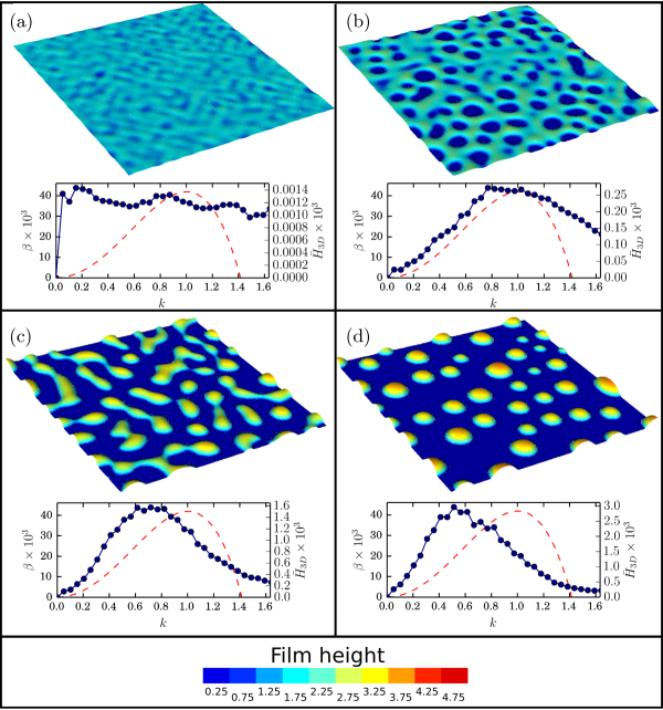
Figure 11: Time evolution of a film breakup in 3D, with $h_{0}=0.5$ and all parameters otherwise identical to the simulation presented in Fig. 9. The color shows the logarithm of the height of the interface above the substrate. The associated Fourier spectrum is shown below each image; these data are averaged over 10 instances, and smoothed with a 5 point running average: (a) $t=0.0$, (b) $t=45$, (c) $t=134$, and (d) $t=301$.

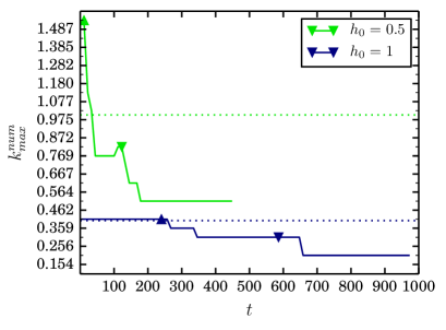
Figure 12: Comparison of $k_{\text{max}}^{\text{num}}$ as a function of time for 3D films with initial thickness $h_{0}=1$ (blue) and $h_{0}=0.5$ (green). The blue curve is identical to that seen in Fig. 10. The blue (green) triangles show the times at which the first holes appear, and the inverted ones show the times at which droplets begin to form. The blue (green) dashed lines show the corresponding values of $k_{\text{max}}$. $\mbox{Oh}=0.487$, and $\theta_{\text{eq}}=0.439\pi$ for both simulation sets.

In this paper, we have demonstrated a computationally efficient method for including fluid-solid interactions into direct numerical simulations. This method is found to perform as well as the body force formulation MahadyvdW15 , while requiring a significantly smaller computational effort. The two methods were compared by considering contact angles of equilibrium drops in 2D, where both methods perform similarly in terms of convergence with mesh refinement, as well as in terms of the behavior when the equilibrium film thickness, $h^{\ast}$, is reduced. The computational complexity required is however dramatically reduced for the presently considered method.

With the established improvement in computational performance, we are now able to study the instability of films due to fluid-solid interaction using direct numerical simulations to gain a quantitative understanding of the evolution of the instability, film rupture, and the post-rupture dewetting process. We compare the results of direct simulations with the linear stability analysis (LSA) of the long-wave formulation (L-W), and find that when contact angle, $\theta_{\text{eq}}$, is larger, there is a significant difference with the predictions of the LSA. We also demonstrate that a reduction in the film thickness does not reduce the differences between the LSA and direct simulations, as the typical in-plane lengthscale decreases even faster than the out-of-plane one (film thickness).

Finally, we study breakup of a film in both 2D and 3D. We consider the evolution of the emerging length scales by computing the discrete Fourier transform (DFT) of the fluid profile. 2D films are characterized by a two stage evolution, and 3D films by a three stage one; for both cases, the initial phase exhibits a DFT with a peak, $k_{\text{max}}^{\text{num}}$, near $k_{\text{max}}$ from the LSA, and each successive stage is associated with a decrease in $k_{\text{max}}^{\text{num}}$, and correspondingly, an increase in the emerging length scales. When a flat film is perturbed by small perturbations, the simulations illustrate the dynamics of dewetting, the formation of ‘dry spots’, and the subsequent coarsening due to inertial effects. When studying the effect of the contact angle for 2D films, we find that the dewetting morphology depends on the contact angle; particularly, the agreement between the simulation results and the predicted fastest growing unstable mode from the LSA deteriorates for large contact angles after the formation of the first expanding holes. When studying the breakup of films in the presence of significant inertial effects, so that characteristic Ohnesorge number, Oh, is small, we find that the long term preference for a specific wavenumber is weaker when compared with the larger Oh, resulting in an increased degree of disorder in the distribution of emerging patterns.

The speed and simplicity of the implementation of the method presented in this paper opens up the possibility of studying a variety of problems involving thin films and other geometries that have not been studied extensively so far by direct numerical simulations. Our numerical method allows, for the first time, for the simulation of arbitrary contact angles (including those greater than $\pi/2$), and film breakup, including inertial effects. While we have studied the influence of varying contact angle and Oh in 2D films, we leave the exhaustive parameter study of 3D films for a future work.

Acknowledgments This work was partially supported by the NSF Grants DMS-1320037 and CBET-1235710.

References

- (1) L. Kondic, J. Diez, P. Rack, Y. Guan, and J. Fowlkes, “Nanoparticle assembly via the dewetting of patterned thin metal lines: Understanding the instability mechanism,” Phys. Rev. E, vol. 79, p. 026302, 2009.
- (2) J. D. Fowlkes, L. Kondic, J. Diez, and P. D. Rack, “Self-Assembly versus Directed Assembly of Nanoparticles via Pulsed Laser Induced Dewetting of Patterned Metal Films,” Nano Lett., vol. 11, p. 2478, 2011.
- (3) J. Fowlkes, N. Roberts, Y. Wu, J. Diez, A. González, C. Hartnett, K. Mahady, S. Afkhami, L. Kondic, and P. Rack, “Hierarchical nanoparticle ensembles synthesized by liquid phase directed self–assembly,” Nano Lett., vol. 14, p. 774, 2014.
- (4) A. G. González, J. A. Diez, Y. Wu, J. Fowlkes, P. Rack, and L. Kondic, “Instability of Liquid Cu films on a SiO2 Substrate,” Langmuir, vol. 29, p. 9378, 2013.
- (5) G. R. Fleming and M. Ratner, “Grand challenges in basic energy sciences,” Phys. Today, vol. 61, p. 28, 2008.
- (6) S. A. Maier, P. G. Kik, H. A. Atwater, S. Meltzer, E. Harel, B. E. Koel, and A. A. Requicha, “Local detection of electromagnetic energy transport below the diffraction limit in metal nanoparticle plasmon waveguide,” Nat. Mat., vol. 2, p. 229, 2003.
- (7) S. Sun, C. Murray, D. Weller, L. Folks, and A. Moser, “Monodisperse FePt nanoparticles and ferromagnetic FePt nanocrystal superlattices,” Science, vol. 287, p. 1989, 2000.
- (8) S. Maier, Plasmonics: Fundamentals and Applications. New York: Springer-Verlag, 2007.
- (9) S. Baderi, “Colloquium: Opportunities in Nanomagnetism,” Rev. Mod. Phys., vol. 78, p. 1, 2006.
- (10) Y. Min, M. Akbulut, K. Kristiansen, Y. Golan, and J. Israelachvili, “The role of interparticle and external forces in nanoparticle assembly,” Nat. Mat., vol. 7, p. 527, 2008.
- (11) N. Roberts, J. Fowlkes, K. Mahady, S. Afkhami, L. Kondic, and P. Rack, “Directed assembly of one- and two-dimensional nanoparticle arrays from pulsed laser induced dewetting of square waveforms,” ACS Appl. Mater. Interfaces, vol. 5, p. 4450, 2013.
- (12) K. Mahady, S. Afkhami, and L. Kondic, “On the influence of initial geometry on the evolution of fluid filaments,” Phys. Fluids, vol. 27, p. 092104, 2015.
- (13) S. Sharma and A. Jameel, “Nonlinear stability, rupture, and morphological phase separation of thin fluid films on apolar and polar substrates,” J. Colloid Interface Sci., vol. 161, p. 190, 1993.
- (14) A. Ghatak, R. Khanna, and A. Sharma, “Dynamics and morphology of holes in dewetting thin films,” J. Colloid Interface Sci., vol. 212, p. 483, 1999.
- (15) A. Sharma, “Many paths to dewetting in thin films: anatomy and physiology of surface instability,” Eur. Phys. J. E, vol. 12, p. 397, 2003.
- (16) R. V. Craster and O. Matar, “Dynamics and stability of thin liquid films,” Rev. Mod. Phys., vol. 81, p. 1131, 2009.
- (17) L. W. Schwartz and R. R. Eley, “Simulation of droplet motion on low-energy and heterogeneous surfaces,” J. Colloid Interface Sci., vol. 202, p. 173, 1998.
- (18) J. Diez and L. Kondic, “On the breakup of fluid films of finite and infinite extent,” Phys. Fluids, vol. 19, p. 072107, 2007.
- (19) J. Eggers, “Contact line motion for partially wetting fluids,” Phys. Rev. E, vol. 72, p. 061605, 2005.
- (20) L. M. Hocking, “A moving fluid interface. Part 2. The removal of the force singularity by a slip flow,” J. Fluid Mech., vol. 79, p. 209, 1977.
- (21) A. Münch, B. Wagner, and T. Witelski, “Lubrication models with small to large slip lengths,” J. Eng. Math., vol. 53, p. 359, 2005.
- (22) S. Afkhami, S. Zaleski, and M. Bussmann, “A mesh-dependent model for applying dynamic contact angles to VOF simulations,” J. Comp. Phys., vol. 228, p. 5370, 2009.
- (23) Y. Shikhmurzaev, “Moving contact lines in liquid/liquid/solid systems,” J. Fluid Mech., vol. 334, p. 211, 1997.
- (24) J. Koplik, J. Banavar, and J. Willemsen, “Molecular Dynamics of Poiseuille Flow and moving contact lines,” Phys. Rev. Lett., vol. 60, p. 1282, 1988.
- (25) P. A. Thompson and M. O. Robbins, “Simulations of Contact-line motion: slip and the dynamic contact angle,” Phys. Rev. Lett., vol. 63, p. 766, 1989.
- (26) P. A. Thompson and S. M. Troian, “A general boundary condition for liquid flow at solid surfaces,” Nature, vol. 389, p. 360, 1997.
- (27) W. Ren and W. E, “Boundary conditions for the moving contact line problem,” Phys. Fluids, vol. 19, p. 022101, 2007.
- (28) R. Seemann, S. Herminghaus, and K. Jacobs, “Dewetting patterns and molecular forces: a reconciliation,” Phys. Rev. Lett., vol. 86, p. 5534, 2001.
- (29) J. Becker, G. Grün, R. Seemann, H. Mantz, K. Jacobs, K. R. Mecke, and R. Blossey, “Complex dewetting scenarios captured by thin-film models,” Nat. Mat., vol. 2, p. 59, 2003.
- (30) V. Ajaev and D. Willis, “Thermocapillary flow and rupture in films of molten metal on a substrate,” Phys. Fluids, vol. 15, p. 3144, 2003.
- (31) J. Trice, D. Thomas, C. Favazza, R. Sureshkumar, and R. Kalyanaraman, “Novel Self-Organization Mechanism in Ultrathin Liquid Films: Theory and Experiment,” Phys. Rev. Lett., vol. 101, p. 017802, 2008.
- (32) M. Fuentes-Cabrera, B. Rhodes, J. Fowlkes, A. López-Benzanilla, H. Terrones, M. Simpson, and P. Rack, “Molecular dynamics study of the dewetting of copper on graphite and graphene: Implications for nanoscale self-assembly,” Phys. Rev. E, vol. 83, p. 041603, 2011.
- (33) M. Khenner, S. Yadavali, and R. Kalyanaraman, “Formation of organized nanostructures from unstable bilayers of thin metallic liquids,” Phys. Fluids, vol. 23, p. 122015, 2011.
- (34) A. Habenicht, M. Olapinski, F. Burmeister, P. Leiderer, and J. Boneberg, “Jumping Nanodroplets,” Science, vol. 309, p. 2043, 2005.
- (35) J. Boneberg, A. Habenicht, D. Benner, P. Leiderer, M. Trautvetter, C. Pfahler, A. Plettl, and P. Ziemann, “Jumping nanodroplets: a new route towards metallic nano-particles,” Appl. Phys. A, vol. 93, no. 2, pp. 415–419, 2008.
- (36) M. Fuentes-Cabrera, B. Rhodes, M. Baskes, H. Terrones, J. Fowlkes, M. Simpson, and P. Rack, “Controlling the Velocity of Jumping Nanodroplets Via Their Initial Shape and Temperature,” ACS Nano, vol. 5, p. 7130, 2011.
- (37) S. Afkhami and L. Kondic, “Numerical simulation of ejected molten metal nanoparticles liquified by laser irradiation: Interplay of geometry and dewetting,” Phys. Rev. Lett., vol. 111, p. 034501, 2013.
- (38) J. H. Snoeijer, “Free-surface flows with large slope: Beyond lubrication theory,” Phys. Fluids, vol. 18, p. 021701, 2006.
- (39) A. Oron, S. H. Davis, and S. G. Bankoff, “Long-scale evolution of thin liquid films,” Rev. Mod. Phys., vol. 69, p. 931, 1997.
- (40) R. V. Craster and O. K. Matar, “Dynamics and stability of thin liquid films,” Rev. Mod. Phys., vol. 81, p. 1131, 2009.
- (41) K. Mahady, S. Afkhami, and L. Kondic, “A volume of fluid method for simulating fluid/fluid interfaces in contact with solid boundaries,” J. Comp. Phys., vol. 294, p. 243, 2015.
- (42) J. Jacqmin, “Calculation of two-phase Navier-Stokes flows using phase field modeling,” J. Comp. Phys., vol. 155, p. 96, 1999.
- (43) J. Jacqmin, “Contact-line dynamics of a diffuse fluid interface,” J. Fluid Mech., vol. 402, p. 57, 2000.
- (44) P. Yue, C. Zhou, and J. Feng, “Sharp-interface limit of the Cahn-–Hilliard model for moving contact lines,” J. Fluid Mech., vol. 645, p. 279, 2010.
- (45) J. N. Israelachvili, Intermolecular and surface forces. New York: Academic Press, 1992. second edition.
- (46) J. Diez, A. Gonzalez, and L. Kondic, “On the breakup of fluid rivulets,” Phys. Fluids, vol. 21, p. 082105, 2009.
- (47) J. U. Brackbill, D. B. Kothe, and C. Zemach, “A continuum method for modeling surface tension,” J. Comp. Phys., vol. 100, p. 335, 1992.
- (48) S. Popinet, “The Gerris flow solver.” http://gfs.sourceforge.net/, 2012. 1.3.2.
- (49) S. Popinet, “An accurate adaptive solver for surface-tension-driven interfacial flows,” J. Comp. Phys., vol. 228, p. 5838, 2009.
- (50) K. Mahady, S. Afkhami, J. Diez, and L. Kondic, “Comparison of Navier-Stokes simulations with long-wave theory: Study of wetting and dewetting,” Phys. Fluids, vol. 25, p. 112103, 2013.
- (51) S. B. G. O’Brien and L. W. Schwartz, Theory and modeling of thin film flows. New York: Encyclopedia of Surface and Colloid Science, Marcel Dekker, 2002.
- (52) S. Nesic, C. R., M. E., and L. Kondic, “Fully nonlinear dynamics of stochastic thin-film dewetting,” Phys. Rev. E, vol. 92, p. 061002(R), 2015.