Induced fermionic current by a magnetic flux in a cosmic string spacetime at finite temperature

Abstract

Here we analyze the finite temperature expectation values of the charge and current densities for a massive fermionic quantum field with nonzero chemical potential, $\mu$, induced by a magnetic flux running along the axis of an idealized cosmic string. These densities are decomposed into the vacuum expectation values and contributions coming from the particles and antiparticles. Specifically the charge density is an even periodic function of the magnetic flux with the period equal to the quantum flux and an odd function of the chemical potential. The only nonzero component of the current density corresponds to the azimuthal current and it is an odd periodic function of the magnetic flux and an even function of the chemical potential. Both analyzed are developed for the cases where $|\mu|$ is smaller than the mass of the field quanta, $m$.

PACS numbers: 03.70.+k, 11.10.Wx, 11.27.+d, 98.80.Cq

1 Introduction

Cosmic strings are among the most important class of linear topological defects with the conical geometry outside the core [1]. The formation of these type of topologically stable structures during the cosmological expansion is predicted in most interesting models of high energy physics. They have a number of interesting observable consequences, the detection of which would provide an important link between cosmology and particle physics.

In quantum field theory, the conical topology of the spacetime due to the presence of a cosmic string causes a number of interesting physical effects. In particular, many authors have considered the vacuum polarization effects for scalar, fermionic and vector fields induced by a planar angle deficit. In addition to the deficit angle parameter, the physical origin of a cosmic string is characterized by the gauge field flux parameter describing a magnetic flux running along the string’s core. The latter induces additional polarization effects for charged fields. [2]-[9] Though the gauge field strength vanishes outside the string’s core, the nonvanishing vector potential leads to Aharonov-Bohm-like effects on scattering cross sections and on particle production rates around the cosmic string. [10]. For charged fields, the magnetic flux along the string core induces nonzero vacuum expectation value of the current density. The latter, in addition to the expectation values of the field squared and the energy-momentum tensor, is among the most important local characteristics of the vacuum state for quantum fields. The azimuthal current density for scalar and fermionic fields, induced by a magnetic flux in the geometry of a straight cosmic string, has been investigated in Ref.s Srir01-Brag14.

Here we shall consider the effects of the finite temperature and nonzero chemical potential on the expectation values of the charge and current densities for a massive fermionic field in the geometry of a straight cosmic string for arbitrary values of the planar angle deficit.

2 Geometry and Fermionic Modes

The background geometry corresponding to a straight cosmic string lying along the $z$-axis can be written through the line element

$$ds^{2}=dt^{2}-dr^{2}-r^{2}d\phi^{2}-dz{}^{2}\ ,$$ (1)

where $r\geqslant 0$, $0\leqslant\phi\leqslant\phi_{0}=2\pi/q$, $-\infty<t<+\infty$. The parameter $q\geqslant 1$ codifies the planar angle deficit. In the presence of an external electromagnetic field with the vector potential $A_{\mu}$, the dynamics of a massive charged spinor field in curved spacetime is described by the Dirac equation,

$$(i\gamma^{\mu}{\mathcal{D}}_{\mu}-m)\psi=0\ ,\ {\mathcal{D}}_{\mu}=\partial_{\mu}+\Gamma_{\mu}+ieA_{\mu},$$ (2)

where $\gamma^{\mu}$ are the Dirac matrices in curved spacetime and $\Gamma_{\mu}$ are the spin connections. For the geometry at hand the gamma matrices can be taken in the form

$$\gamma^{0}=\left(\begin{array}[]{cc}1&0\\ 0&-1\end{array}\right),\;\gamma^{l}=\left(\begin{array}[]{cc}0&\rho^{l}\\ -\rho^{l}&0\end{array}\right),$$ (3)

where the $2\times 2$ matrices $\rho^{l}$ are

$$\rho^{1}=\left(\begin{array}[]{cc}0&e^{-iq\phi}\\ e^{iq\phi}&0\end{array}\right)\ ,\ \rho^{2}=-\frac{i}{r}\left(\begin{array}[]{cc}0&e^{-iq\phi}\\ -e^{iq\phi}&0\end{array}\right)\ ,\ \rho^{3}=\left(\begin{array}[]{cc}1&0\\ 0&-1\end{array}\right)\ .$$ (4)

We shall admit the existence of a gauge field with a constant vector potential as

$$A_{\mu}=(0,0,A_{\phi},0)\ .$$ (5)

The azimuthal component $A_{\phi}$ is related to an infinitesimal thin magnetic flux, $\Phi$, running along the string by $A_{\phi}=-q\Phi/(2\pi)$.

The field operator can be expanded in term of a complete set of normalized positive- and negative-energy solution $\{\psi_{\sigma}^{(+)},\psi_{\sigma}^{(-)}\}$ of (2), specified by a set of quantum numbers $\sigma$, as:

$$\psi=\sum_{\sigma}[\hat{a}_{\sigma}\psi_{\sigma}^{(+)}+\hat{b}_{\sigma}^{+}\psi_{\sigma}^{(-)}]\ ,$$ (6)

where $\hat{a}_{\sigma}$ and $\hat{b}_{\sigma}^{+}$ represent the annihilation and creation operators corresponding to particles and antiparticles respectively.

Here, we are interested in the effects of the presence of the cosmic string and magnetic flux on the expectation values of the charge and current densities assuming that the field is in thermal equilibrium at finite temperature $T$. The standard form of the density matrix for the thermodynamical equilibrium distribution at temperature $T$ is

$$\hat{\rho}=Z^{-1}e^{-\beta(\hat{H}-\mu^{\prime}\hat{Q})},\;\beta=1/T\ \ ,\ {\rm and}\ Z=\mathrm{tr}[e^{-\beta(\hat{H}-\mu^{\prime}\hat{Q})}]\ ,$$ (7)

where $\hat{H}$ is the Hamilton operator, $\hat{Q}$ denotes a conserved charge and $\mu^{\prime}$ is the corresponding chemical potential. The thermal average of the creation and annihilation operators are given by:

$$\mathrm{tr}[\hat{\rho}\hat{a}_{\sigma}^{+}\hat{a}_{\sigma^{\prime}}] = \frac{\delta_{\sigma\sigma^{\prime}}}{e^{\beta(\varepsilon_{\sigma}^{(+)}-\mu)}+1},$$

$$\mathrm{tr}[\hat{\rho}\hat{b}_{\sigma}^{+}\hat{b}_{\sigma^{\prime}}] = \frac{\delta_{\sigma\sigma^{\prime}}}{e^{\beta(\varepsilon_{\sigma}^{(-)}+\mu)}+1},$$ (8)

where $\mu=e\mu^{\prime}$ and $\pm\varepsilon_{\sigma}^{(\pm)}$ with $\varepsilon_{\sigma}^{(\pm)}>0$, are the energies corresponding to the modes $\psi_{\sigma}^{(\pm)}$.

The expectation value of the fermionic current density given by $\left\langle j^{\nu}\right\rangle=e\,\mathrm{tr}[\hat{\rho}\bar{\psi}(x)\gamma^{\nu}\psi(x)]$, can be expressed by

$$\left\langle j^{\nu}\right\rangle=\left\langle j^{\nu}\right\rangle_{0}+\sum_{\chi=+,-}\left\langle j^{\nu}\right\rangle_{\chi},$$ (9)

where

$$\left\langle j^{\nu}\right\rangle_{0}=e\sum_{\sigma}\bar{\psi}_{\sigma}^{(-)}(x)\gamma^{\nu}\psi_{\sigma}^{(-)}(x),$$ (10)

is the vacuum expectation value and

$$\left\langle j^{\nu}\right\rangle_{\pm}=\pm e\sum_{\sigma}\frac{\bar{\psi}_{\sigma}^{(\pm)}\gamma^{\nu}\psi_{\sigma}^{(\pm)}}{e^{\beta(\varepsilon_{\sigma}^{(\pm)}\mp\mu)}+1}.$$ (11)

Here, $\left\langle j^{\nu}\right\rangle_{\pm}$ is the part in the expectation value coming from the particles for the upper sign and from the antiparticles for the lower sign.

We shall use the normalized fermionic modes found in Ref. Beze13 specified by the set of quantum numbers $\sigma=(\lambda,k,j,s)$ with

$$\lambda\geqslant 0,\;-\infty<k<+\infty,\;j=\pm 1/2,\pm 3/2,\ldots,\;s=\pm 1.$$ (12)

These functions are expressed as

$$\psi_{\sigma}^{(\pm)}(x)=C_{\sigma}^{(\pm)}e^{\mp iEt+ikz+iqj\phi}\left(\begin{array}[]{c}J_{\beta_{j}}(\lambda r)e^{-iq\phi/2}\\ sJ_{\beta_{j}+\epsilon_{j}}(\lambda r)e^{iq\phi/2}\\ \pm\frac{k-is\epsilon_{j}\lambda}{E\pm m}J_{\beta_{j}}(\lambda r)e^{-iq\phi/2}\\ \mp s\frac{k-is\lambda\epsilon_{j}}{E\pm m}J_{\beta_{j}+\epsilon_{j}}(\lambda r)e^{iq\phi/2}\end{array}\right)\ ,$$ (13)

where $J_{\nu}(x)$ is the Bessel function, $|C_{\sigma}^{(\pm)}|^{2}=\frac{q\lambda(E\pm m)}{16\pi^{2}E}$ and

$$E=\varepsilon_{\sigma}^{(\pm)}=\sqrt{\lambda^{2}+k^{2}+m^{2}}\ ,\ \beta_{j}=q|j+\alpha|-\epsilon_{j}/2\ ,\;\alpha=eA_{\phi}/q=-\Phi/\Phi_{0}\ ,$$ (14)

with $\epsilon_{j}=\mathrm{sgn}(j+\alpha)$ and $\Phi_{0}=2\pi/e$ being the flux quantum.

3 Charge Density

We start with the charge density corresponding to the $\nu=0$ component of (9). In Ref. Beze13 we have explicitly shown that the formal expression for the vacuum expectation value of charge density is given in terms of a divergent integral. In order to obtain a finite and well defined result we introduced a cutoff function. With this cutoff the integral could be evaluated. Our next steps were to subtract the Minkowskian part $(\alpha_{0}=0,\ q=1)$ and to remove the cutoff function. As final result a vanishing value for the renormalized charge density was obtained.

Substituting the mode functions (13) into (11), for the contributions coming from the particles and antiparticles we get

$$\left\langle j^{0}\right\rangle_{\pm}=\pm\frac{eq}{8\pi^{2}}\sum_{\sigma}\lambda\frac{J_{\beta_{j}}^{2}(\lambda r)+J_{\beta_{j}+\epsilon_{j}}^{2}(\lambda r)}{e^{\beta(E\mp\mu)}+1},$$ (15)

where we use the notation

$$\sum_{\sigma}=\int_{-\infty}^{+\infty}dk\int_{0}^{\infty}d\lambda\ \sum_{s=\pm 1}\sum_{j}\ .$$ (16)

In the case $\mu=0$ the contributions from the particles and antiparticles cancel each other and the total charge density,

$$\left\langle j^{0}\right\rangle=\left\langle j^{0}\right\rangle_{+}+\left\langle j^{0}\right\rangle_{-},$$ (17)

is zero. From (15) one can see that the charge density is an even periodic function of the parameter $\alpha$ with the period equal to 1. Consequently the charge density is a periodic function of the magnetic flux with the period equal to the quantum flux. If we present this parameter as

$$\alpha=n_{0}+\alpha_{0},\;|\alpha_{0}|\leqslant 1/2,$$ (18)

with $n_{0}$ being an integer, then the current density depends on $\alpha_{0}$ alone.

Here in this paper we shall consider only the case $|\mu|<m$. By using the expansion $(e^{y}+1)^{-1}=-\sum_{n=1}^{\infty}(-1)^{n}e^{-ny}$, the charge densities for particles and antiparticles can be presented in the form

$$\left\langle j^{0}\right\rangle_{\pm} = \mp\frac{eq\beta}{4\pi^{2}r^{4}}\ \sum_{n=1}^{\infty}(-1)^{n}ne^{\pm n\beta\mu}\int_{0}^{\infty}dx\,x$$ (19)

$$\times F(q,\alpha_{0},x)e^{-m^{2}r^{2}/2x-(1+n^{2}\beta^{2}/2r^{2})x}\ ,$$

where the notation

$$F(q,\alpha_{0},x)=\sum_{j}\ \left[I_{\beta_{j}}(x)+I_{\beta_{j}+\epsilon_{j}}(x)\right],$$ (20)

is introduced. In Ref. Beze10b we have shown that

$$F(q,\alpha_{0},x) = \frac{4}{q}\left[\frac{e^{x}}{2}+\sum_{k=1}^{[q/2]}(-1)^{k}c_{k}\cos\left(2\pi k\alpha_{0}\right)e^{x\cos(2\pi k/q)}\right.$$ (21)

$$\left.+\frac{q}{\pi}\int_{0}^{\infty}dy\frac{h(q,\alpha_{0},2y)\sinh y}{\cosh(2qy)-\cos(q\pi)}e^{-x\cosh{(2y)}}\right]\ ,$$

where $[q/2]$ means the integer part of $q/2$ and the notation

$$h(q,\alpha_{0},x)=\sum_{\chi=\pm 1}\cos\left[\left(1/2+\chi\alpha_{0}\right)q\pi\right]\sinh\left[\left(1/2-\chi\alpha_{0}\right)qx\right],$$ (22)

is assumed. Here and in what follows we use the notations

$$c_{k}=\cos{(\pi k/q),\;s}_{k}=\sin{(\pi k/q).}$$ (23)

Substituting (21) into (19), after integration over $x$, we find the expression

$$\left\langle j^{0}\right\rangle_{\pm} = \left\langle j^{0}\right\rangle_{\mathrm{M}\pm}\mp\frac{2em^{4}\beta}{\pi^{2}}\ \sum_{n=1}^{\infty}(-1)^{n}ne^{\pm n\beta\mu}$$ (24)

$$\times\left[\sum_{k=1}^{[q/2]}(-1)^{k}c_{k}\cos\left(2\pi k\alpha_{0}\right)f_{2}(m\beta s_{n}(r/\beta,k/q))\right.$$

$$\left.+\frac{q}{\pi}\int_{0}^{\infty}dy\frac{\sinh\left(y\right)h(q,\alpha_{0},2y)}{\cosh(2qy)-\cos(q\pi)}f_{2}(m\beta c_{n}(r/\beta,y))\right],$$

where

$$\left\langle j^{0}\right\rangle_{\mathrm{M}\pm}=\mp\frac{e\beta m^{4}}{\pi^{2}}\sum_{n=1}^{\infty}(-1)^{n}ne^{\pm n\beta\mu}f_{2}(nm\beta),$$ (25)

is the corresponding charge density in Minkowski spacetime in the absence of the magnetic flux and the cosmic string ($\alpha_{0}=0$, $q=1$). Here we have introduced the notations

$$f_{\nu}(x)=x^{-\nu}K_{\nu}(x),$$ (26)

with $K_{\nu}(x)$ being the MacDonald function and

$$s_{n}(x,y)=\sqrt{n^{2}+4x^{2}\sin^{2}(\pi y)},\ c_{n}(x,y)=\sqrt{n^{2}+4x^{2}\cosh^{2}y}\ .$$ (27)

For the total charge density one gets

$$\left\langle j^{0}\right\rangle = -\frac{4em^{4}\beta}{\pi^{2}}\ \sum_{n=1}^{\infty}(-1)^{n}n\sinh(n\beta\mu)\left[\frac{1}{2}f_{2}(m\beta n)\right.$$ (28)

$$+\sum_{k=1}^{[q/2]}(-1)^{k}c_{k}\cos\left(2\pi k\alpha_{0}\right)f_{2}(m\beta s_{n}(r/\beta,k/q))$$

$$\left.+\frac{q}{\pi}\int_{0}^{\infty}dy\frac{h(q,\alpha_{0},2y)\sinh y}{\cosh(2qy)-\cos(q\pi)}f_{2}(m\beta c_{n}(r/\beta,y))\right]\ .$$

We present in figure 1, the total charge density as a function of the parameter $\alpha_{0}$ (left panel) and the charge density induced by the string and magnetic flux as a function of the temperature (right panel). The numbers near the curves correspond to the values of the parameter $q$. The graphs on the left panel are plotted for $T/m=1$, $mr=0.25$, and $\mu/m=0.5$. On the right panel, the full and dashed curves correspond to the values $\alpha_{0}=1/2$ and $\alpha_{0}=0$, respectively (note that for $q=1$, $\alpha_{0}=0$ one has $\left\langle j^{0}\right\rangle-\left\langle j^{0}\right\rangle_{\mathrm{M}}=0$). For the graphs on the right panel we have taken $\mu/m=0.5$ and $mr=1/8$.

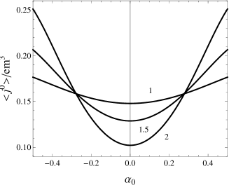
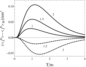
Figure 1: The total charge density as a function of the parameter $\alpha_{0}$ (left panel) and the charge density induced by the string and magnetic flux as a function of the temperature (right panel). The numbers near the curves correspond to the values of the parameter $q$. The graphs on the left panel are plotted for $T/m=1$, $mr=0.25$, and $\mu/m=0.5$ . On the right panel, the full and dashed curves correspond to the values $\alpha_{0}=1/2$ and $\alpha_{0}=0$, respectively. For the graphs on the right panel we have taken $\mu/m=0.5$ and $mr=1/8$

At large distance and high temperature the Minkowski contribution dominates and the one induced by the cosmic string and magnetic flux are exponentially suppressed.[18]. In figure 2, we present the charge density as a function of the radial coordinate. The full and dashed lines correspond to the values $\alpha_{0}=1/2$ and $\alpha_{0}=0$, respectively. The numbers near the curves present the values of the parameter $q$. The graphs are plotted for $T/m=1$ and $\mu/m=0.5$.

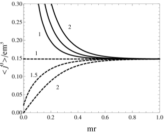
Figure 2: The charge density versus the radial coordinate. The full and dashed lines correspond to the values $\alpha_{0}=1/2$ and $\alpha_{0}=0$, respectively. The numbers near the curves present the values of the parameter $q$. The graphs are plotted for $T/m=1$ and $\mu/m=0.5$.

4 Azimuthal Current

Now we turn to the investigation of the current density. The only nonzero component corresponds to the azimuthal current ($\nu=2$ in (9)). By taking into account the expression for the mode functions, from (11) for the physical components of the current densities of the particles and antiparticles, $\left\langle j_{\phi}\right\rangle_{\pm}=r\left\langle j^{2}\right\rangle_{\pm}$, we get

$$\left\langle j_{\phi}\right\rangle_{\pm}=\frac{eq}{4\pi^{2}}\sum_{\sigma}\epsilon_{j}\frac{\lambda^{2}}{E}\frac{J_{\beta_{j}}(\lambda r)J_{\beta_{j}+\epsilon_{j}}(\lambda r)}{e^{\beta(E\mp\mu)}+1},$$ (29)

where the upper and lower signs correspond to the particles and antiparticles respectively and the collective summation is defined by (16).

For the case $|\mu|<m$, by using the same expansion for the denominator as we did in the previous case, the current densities (29) reads

$$\left\langle j_{\phi}\right\rangle_{\pm}=-\frac{eq}{2\pi^{2}r^{3}}\sum_{n=1}^{\infty}(-1)^{n}e^{\mp n\beta\mu}\int_{0}^{\infty}dx\,xe^{-m^{2}r^{2}/(2x)-(1+n^{2}\beta^{2}/(2r^{2}))x}G(q,\alpha_{0},x),$$ (30)

with the notation

$$G(q,\alpha_{0},x)=\sum_{j}\ \left[I_{\beta_{j}}(x)-I_{\beta_{j}+\epsilon_{j}}(x)\right].$$ (31)

By using the integral representation for the modified Bessel function we can write

$$G(q,\alpha_{0},x) = \frac{4}{q}\sideset{}{{}^{\prime}}{\sum}_{k=1}^{[q/2]}(-1)^{k}s_{k}\sin\left(2\pi k\alpha_{0}\right)e^{x\cos(2\pi k/q)}$$ (32)

$$+\frac{4}{\pi}\int_{0}^{\infty}dy\ \frac{g(q,\alpha_{0},2y)\cosh y}{\cosh(2qy)-\cos(q\pi)}e^{-x\cosh{(2y)}},$$

with the notation

$$g(q,\alpha_{0},x)=\sum_{\chi=\pm 1}\chi\cos\left[\left(1/2+\chi\alpha_{0}\right)q\pi\right]\cosh\left[\left(1/2-\chi\alpha_{0}\right)qx\right]\ .$$ (33)

The prime on the summation sign in (32) means that, in the case where $q$ is an even number, the term with $k=q/2$ should be taken with the coefficient 1/2.

Substituting (32) into (30), after integrating over $x$, we obtain

$$\left\langle j_{\phi}\right\rangle_{\pm} =-\frac{4em^{4}r}{\pi^{2}}\sum_{n=1}^{\infty}(-1)^{n}e^{\mp n\beta\mu}$$

$$\times\left[\ \sideset{}{{}^{\prime}}{\sum}_{k=1}^{[q/2]}(-1)^{k}s_{k}\sin\left(2\pi k\alpha_{0}\right)f_{2}\left(m\beta s_{n}(r/\beta,k/q)\right)\right.$$

$$+\left.\frac{q}{\pi}\int_{0}^{\infty}dy\ \frac{\cosh\left(y\right)g(q,\alpha_{0},2y)}{\cosh(2qy)-\cos(q\pi)}f_{2}(m\beta c_{n}(r/\beta,y))\right],$$ (34)

where the functions in the arguments of $f_{2}(x)$ are defined by (27). For the case $q=1$, i.e. in the absence of conical defect, the above expression reduces to

$$\left\langle j_{\phi}\right\rangle_{\pm} =\frac{4em^{4}r}{\pi^{3}}\sin(\alpha_{0}\pi)\sum_{n=1}^{\infty}(-1)^{n}e^{\mp n\beta\mu}$$

$$\times\int_{0}^{\infty}dy\,\cosh(2\alpha_{0}y)f_{2}\left(m\beta c_{n}(r/\beta,y)\right)\ .$$ (35)

Taking into account the expression for the vacuum expectation value of the current density from [17], the total current density reads

$$\left\langle j_{\phi}\right\rangle =-\frac{8em^{4}r}{\pi^{2}}\sideset{}{{}^{\prime}}{\sum}_{n=0}^{\infty}(-1)^{n}\cosh(n\beta\mu)$$

$$\times\left[\ \sideset{}{{}^{\prime}}{\sum}_{k=1}^{[q/2]}(-1)^{k}s_{k}\sin\left(2\pi k\alpha_{0}\right)f_{2}\left(m\beta s_{n}(r/\beta,k/q)\right)\right.$$

$$+\left.\frac{q}{\pi}\int_{0}^{\infty}dy\ \frac{\cosh\left(y\right)g(q,\alpha_{0},2y)}{\cosh(2qy)-\cos(q\pi)}f_{2}\left(m\beta c_{n}(r/\beta,y)\right)\right],$$ (36)

where the prime on the sign of the summation over $n$ means that the term $n=0$ should be taken with the coefficient 1/2. This term corresponds to the vacuum expectation value of the current density, $\left\langle j_{\phi}\right\rangle_{0}$.

Now we would like to analyze the case of a massless field. Because of the condition $|\mu|\leqslant m$, we should also take $\mu=0$. By using the asymptotic expression for the MacDonald function for small argument, the summation over $n$ takes the form $\sideset{}{{}^{\prime}}{\sum}_{n=0}^{\infty}(-1)^{n}\left(n^{2}+x^{2}\right)^{-2}$, that can be expressed in terms of the hyperbolic functions. So we get

$$\left\langle j_{\phi}\right\rangle =-\frac{eT}{2\pi r^{2}}\left[\ \sideset{}{{}^{\prime}}{\sum}_{k=1}^{[q/2]}\frac{(-1)^{k}}{s_{k}^{2}}\sin\left(2\pi k\alpha_{0}\right)h(2rTs_{k})\right.$$

$$\left.+\frac{q}{\pi}\int_{0}^{\infty}dy\ \frac{g(q,\alpha_{0},2y)}{\cosh(2qy)-\cos(q\pi)}\frac{h(2rT\cosh y)}{\cosh^{2}y}\right]\ ,$$ (37)

where we have introduced the function

$$h(x)=\frac{1+\pi x\coth(\pi x)}{\sinh(\pi x)}.$$ (38)

We plot in figure 3, for a massless field with $\mu=0$, the azimuthal current density as a function of the parameter $\alpha_{0}$ (left panel) and as a function of the temperature (right panel). The numbers near the curves correspond to the values of $q$. In the graphs on the left panel we assume $rT=0.25$ and on the right $\alpha_{0}=0.25$.

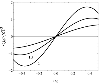
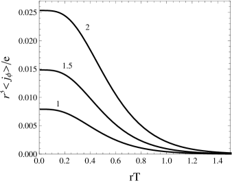
Figure 3: The azimuthal current density for a massless field with zero chemical potential as a function of $\alpha_{0}$ (left panel) and as a function of the temperature (right panel). The numbers near the curves correspond to the values of $q$. For the graphs on the left panel $rT=0.25$ and for the right panel $\alpha_{0}=0.25$.

5 Conclusion

In this paper, we have analyzed the combined effects of the planar angle deficit and the magnetic flux on the charge and current densities for a massive fermionic field at thermal equilibrium considering nonzero chemical potential. These densities are decomposed into the vacuum expectation values and finite temperature contributions, coming from the particles and antiparticles.

For the charge density the renormalized vacuum expectation value vanishes and the expectation value for the particles and antiparticles in the case $|\mu|\leqslant m$ are given by (24). The charge density is an even periodic function of the magnetic flux with period equal to the quantum flux. For the zero chemical potential the contributions from the particles and antiparticles cancel each other and the total charge density, given by (28), vanishes.

The only nonzero component of the expectation value for the current density corresponds to the current along the azimuthal direction. This current vanishes in the absence of the magnetic flux and is an odd periodic function of the latter with the period equal to the quantum flux. The azimuthal current density is an even function of the chemical potential. For the zero chemical potential, the contributions to the total current density from the particles and antiparticles coincide.

References

• [1] A. Vilenkin and E. P. S. Shellard, Cosmic Strings and Other Topological Defects (Cambridge University Press, Cambridge, 1994).
• [2] J. S. Dowker, Phys. Rev. D 36, 3095 (1987).
• [3] J. S. Dowker, Phys. Rev. D 36, 3742 (1987).
• [4] M. E. X. Guimarães and B. Linet, Commun. Math. Phys. 165, 297 (1994).
• [5] J. Spinelly and E. R. Bezerra de Mello, Class. Quantum Grav. 20 874, (2003).
• [6] J. Spinelly and E.R. Bezerra de Mello, Int. J. Mod. Phys. A 17, 4375 (2002).
• [7] J. Spinelly and E. R. Bezerra de Mello, Int. J. Mod. Phys. D 13, 607 (2004).
• [8] J. Spinelly and E. R. Bezerra de Mello, JHEP 09, 005 (2008).
• [9] Yu. A. Sitenko and N. D. Vlasii, Class. Quantum Grav. 29, 095002 (2012).
• [10] M. G. Alford and F. Wilczek, Phys. Rev. Lett. 62, 1071 (1989).
• [11] D. A. Steer and T. Vachaspati, Phys. Rev. D 83, 043528 (2011).
• [12] L. Sriramkumar, Class. Quantum Grav. 18, 1015 (2001).
• [13] Yu. A. Sitenko and N. D. Vlasii, Class. Quantum Grav. 26, 195009 (2009).
• [14] E. R. Bezerra de Mello, Class. Quantum Grav. 27, 095017 (2010).
• [15] E. R. Bezerra de Mello and A. A. Saharian, Eur. Phys. J. C 73, 2532 (2013).
• [16] E. A. F. Bragança, H. F. Santana Mota and E. R. Bezerra de Mello, Int. J. Mod. Phys. D 24, 1550055 (2015).
• [17] E. R. Bezerra de Mello and A. A. Saharian, Eur. Phys. J. C 73, 2532 (2013).
• [18] A. Mohammadi, E. R. Bezerra de Mello and A. A. Saharian, J. Phys. A. Math. Theor. 48 185401 (2015).
• [19] E. R. Bezerra de Mello, V. B. Bezerra, A. A. Saharian and V. M. Bardeghyan, Phys. Rev. D 82, 085033 (2010).