Critical Phenomena of Dynamical Delocalization in Quantum Anderson Map

Abstract

Using a quantum map version of one-dimensional Anderson model, the localization-delocalization transition of quantum diffusion induced by coherent dynamical perturbation is investigated in comparison with quantum standard map. Existence of critical phenomena, which depends on the number of frequency component $M$, is demonstrated. Diffusion exponents agree with theoretical prediction for the transition, but the critical exponent of the localization length deviates from it with increase in the $M$. The critical power $\epsilon_{c}$ of the normalized perturbation at the transition point remarkably decreases as $\epsilon_{c}\sim(M-1)^{-1}$.

I Introduction and Models

The localization phenomena are persistent and robust in one-dimensional disordered systems (1DDS) ishii73 ; lifshiz88 ; stollmann01 . It still remains even in two-dimensional disordered systems. However, if the dimension $d$ of the disordered system is more than 2, the localization becomes unstable, and the localization-delocalization transition (LDT) takes place, and finally an irreversible diffusion sets in when we consider quantum diffusion of an initially localized wavepacket. The critical phenomena of LDT have been extensively studied on the basis of the one-parameter scaling theory (OPST) of the localization by many authors abrahams79 ; macKinnon81 ; slevin97 ; croy11 ; markos06 ; garcia07 . The recent reviews and developments for LDT have been given in a commemorative book abrahams10 , and references therein.

On the other hand, similar localization phenomena were discovered for the quantum kicked rotors (KR) typically exemplified by the quantum standard map (SM), and it can be interpreted as the localization phenomenon of a class of 1DDS in terms of Maryland transformation grempel84 ; casati89 ; ikeda93 ; garcia08 ; tian11 . In this context, the additional dimensionality $(d-1)$ corresponds to the number of the dynamical degrees of freedom $M$ applied to the KR, and the LDT in 1DDS corresponds to the ergodic transition when we consider the dynamically perturbed standard maps. Based upon this correspondence, the critical phenomenon of the LDT was observed for Cesium atoms in optical lattice settings chabe08 ; rodriguez09 .

On the analogy of the standard map’s case, we can expect that the localization in the 1DDS is unstable against the dynamical perturbations. We have proposed the delocalization scenario that the dynamical perturbation to 1DDS in general enhances the localization length and restore the diffusive motion in a strong perturbation regime yamada99 . Considering that electrons are interacting with lattice vibrations, the effect of dynamical perturbation by phonon modes is essential. It models the fundamental dynamical and deterministic process of the quantum electronic motion turning into diffusive one which allows time-irreversible kinetic description.

Here, a basic question arises. Whether the LDT happens in the 1DDS under the interaction with dynamical degrees of freedom, and if it happens, how the nature of LDT changes with increase in the mode number $M$. To answer this we introduce the 1D Anderson map (AM) described by the unitary time-evolution operator

$$\hat{U}_{m}={\rm e}^{-i\Delta T(p)/2\hbar}{\rm e}^{-i\Delta(f(t_{m})V(q)/\hbar)}{\rm e}^{-i\Delta T(p)/2\hbar},$$ (1)

for wave function defined on the discrete lattice site $q(=n)$, where $T(p)=2\cos(p/\hbar)={\rm e}^{-d/dq}+{\rm e}^{+d/dq}$ and $V(q)(=V(n))$ is random on-site potential uniformly distributed over the range $[-W,W]$ yamada04 ; yamada12 . The dynamical perturbation is modeled by the sinusoidal periodic perturbation superposed onto the on-site energy as

$$f(t)=1+\frac{\epsilon}{\sqrt{M}}\sum_{k=1}^{M}\cos(\omega_{k}t),$$ (2)

where $M$ and $\epsilon$ are the number of the frequency component and the strength of the perturbation, respectively. The time evolution by the operator $\hat{U}_{m}$ approximates the unitary evolution of the dynamically perturbed Anderson model,

$$i\hbar\frac{\partial u(n,t)}{\partial t}=u(n-1,t)+u(n+1,t)+f(t)V(n)u(n,t),$$ (3)

for a short time interval $\Delta$ up to the correction of $O(\Delta^{3})$, and the unperturbed Anderson map ($\epsilon=0$) retains the localization properties of the Anderson model yamada04 ; yamada12 . In addition, the numerical verification of the presence of LDT is very hard for the perturbed Anderson model, therefore we examine here the perturbed Anderson map to explore the presence of LDT, where we take $\Delta=1$, typically. Note that the strength of the perturbation is divided by $\sqrt{M}$ so as to make the total power of long-time average independent of $M$, and the frequencies are taken as incommensurate numbers of $O(1)$ frequecy . Replacing by $T(p)=p^{2}/2$ and $V(q)=K\cos(q)$, Eq.(1) turns into the SM, which exhibits the LDT in the momentum space casati89 .

In the perturbed AM, both localation and delocalization have been observed yamada04 ; yamada12 . However, the nature of the transition from the former to the latter was not known, in particular, the presence of critical phenomena in the transition process is still unclear. In this paper, we numerically investigate the critical nature of the LDT in the AM in comparison with the LDT in the SM, which can be analyzed by the OPST chabe08 ; rodriguez09 . In particular, we are interested in the mode number $M$ dependence of the transition, regarding the $M$ with the additional dimension $(d-1)$ according to the interpretation in the case of SM casati89 ; chabe08 . We increase the effective dimensionality $(M+1)=d$ far beyond $3$. It will provide a crucial test for the mean-field theory of the Anderson transition, which regards $d=3$ as the lower bound above which the critical exponents lose the $d-$denendency.

II Subdiffusive properties of wavepacket dynamics at the localization-delocalization transition

For $M=1$, the localization length increases exponentially with the coupling strengeth $\epsilon$, but we could not confirm the presence of delocalized state. However, if $M\geq 2$, we can confirm the presence of critical state, which evidently borders the delocalizing behavior and the localizing one. This will be described closely in the present section.

II.1 Numerical results

Let us introduce the on-site probability $P(n,t)=|u(n,t)|^{2}$. The main tool of our analysis we use the time-dependent mean square displacement (MSD) $m_{2}(t)=<\sum_{n=-\infty}^{\infty}(n-<n>)^{2}P(n,t)>_{\Omega}$ of the propagating wavepacket starting from localized one, $u(n,t=0)=\delta_{n,n_{0}}$, where $<\dots>_{\Omega}$ denotes the ensemble average over different random configuration of $V(n)$. With increase in the perturbation strength, the time-evolution changes from the localized behavior to delocalized one passing through the critical behavior at a certain critical strength $\epsilon=\epsilon_{c}$. (See Fig.1(a) for the result of AM with $M=2$. ) At the critical state the MSD exhibits a power-law asymptotic (subdiffusive) dependence $m_{2}(t)\sim t^{\alpha}$ characterized by the diffusion exponent $\alpha$, which is close to the theoretical value $0.66$ discussed later. Instead of the MSD, we introduce the scaled MSD

$$\Lambda(\epsilon,t)\equiv\frac{m_{2}(\epsilon,t)}{t^{\alpha}}$$ (4)

with respect to the critical behavior $t^{\alpha}$ and show its temporal evolution at various $\epsilon$ including $\epsilon_{c}$ in Fig.1(b). The critical curve indicated by the bold line separates the curves spreading like a fan into the delocalization regime ($\epsilon>\epsilon_{c}$) increasing up to the normal diffusion $m_{2}(t)\to Dt~{}(\Lambda\to t^{1-\alpha})$ and localization regime ($\epsilon<\epsilon_{c}$) decreasing down to the localization length $m_{2}(t)\to\xi~{}(\Lambda\to t^{-\alpha})$. Here, the diffusion constant $D=D(\epsilon)$ and the localization length $\xi=\xi(\epsilon)$ approach to zero and infinity, respectively, as $\epsilon\to\epsilon_{c}$.

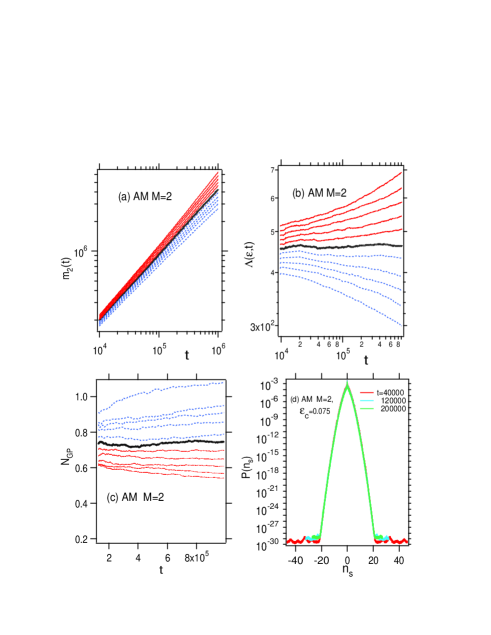
Figure 1: (Color online) The diffusive properties of the wavepacket in the perturbed AM with $M=2$. The system and ensemble sizes are $N=2^{15}\sim 2^{17}$ and $10\sim 100$, respectively, throughout this paper, and we mainly take $W=0.5$ as the disorder strength and $\hbar=0.125$ as the Planck constant, respectively. (a)The double logarithmic plot of $m_{2}(t)$ as a function of time for different values of the perturbation strength $\epsilon$, where the diffusion exponent $\alpha(=0.66)$ is determined by the least-square-fit for $m_{2}(t)$ with the critical case. (b)The scaled MSD $\Lambda(\epsilon,t)$ as a function of time for different values of the perturbation strength $\epsilon$. Note that this is log-log plot. (c)$N_{GP}$ as a function of time for different values of the perturbation strength $\epsilon$. Note that the black thick lines in the panels (a),(b) and (c) show the results at the critical case $\epsilon_{c}=0.075$. The blue dashed curves show the results for $\epsilon<\epsilon_{c}$ in the panels (a), (b) and (c). (d)Semi-log plots of the scaled probability density $P(n_{s}(t))$ as a function of the $n_{s}=n/\sqrt{m_{2}(t)}$ for $t=4\times 10^{4},12\times 10^{4},20\times 10^{4}$ at the critical case. The curves of all cases are well-overlapped.

To clarify the shape of the distribution, in addition to the MSD, we introduce the non-Gaussian parameter (NGP) $N_{GP}$ defined by

$$N_{GP}(t) = \frac{1}{3}\frac{m_{4}(t)}{m_{2}(t)^{2}}-1,$$ (5)

where $m_{4}(t)=\sum(n-<n>)^{4}P(n,t)$. Figure 1(c) depicts the time dependence of NGP for various $\epsilon$. At the critical point the NGP keeps the same nonzero-value, implying that the shape of the distribution function takes a similar non-Gaussian form throughout the time evolution gogolin76 ; ketzmerick97 . Figure 1(d) shows the distribution function $P_{s}(n_{s}(t),t)=P(n,t)dn/dn_{s}(t)$ at several $t$’s as a function of scaled coordinate $n_{s}(t)$ by the spread of the wavepacket for AM with $M=2$ as

$$n_{s}(t)=\frac{n}{\sqrt{m_{2}(t)}}\propto\frac{n}{t^{\alpha/2}}.$$ (6)

Evidently, the scaled representation $P_{s}(n_{s},t)$ does not have explicit $t$ dependence as is expected. Thus we denote the scaled distribution function simply by $P_{s}(n_{s}(t))$.

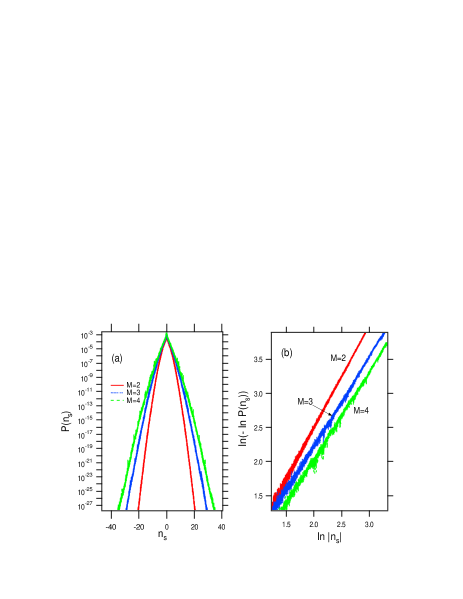
Figure 2: (Color online) (a)The scaled invariant distribution $P(n_{s})$ of AM as the function of $n_{s}=n/\sqrt{m_{2}(t)}$ for $M=2,3,4$ at each critical perturbation strength $\epsilon_{c}$ from the inside to the outside. (b)The plot of $\ln|-\ln P(n_{s})|$ as a function of $|n_{s}|$ in the logarithmic scale. The slopes correspond to the exponent $\beta$ of the stretched Gaussian distribution.

We further investigate the invariant function form of the wavepacket at each critical point of various $M$’s, as seen in Fig.2(a) for AM with $M=2,3,4$. It is suggested that the tail of the scaled invariant shape of the distribution function takes the stretched Gaussian distribution

$$P(n_{s})\sim{\rm exp}(-|n_{s}(t)|^{\beta}),$$ (7)

except for the range close to the origin of the critical state, where $\beta$ is the distribution exponent (streched Gaussian exponent). The tails are shown in 2(b) in the plot of $\ln|-\ln P(n_{s})|$ as a function of $\ln|n_{s}|$ for each case in Fig.2(a). The slopes of the plots correspond to the exponents $\beta$ of the stretched Gaussian distribution, which are decided by the least-square-fit except for the range close to the origin. The $M$-dependence of estimated diffusion exponent $\alpha$ and the stretched Gaussian exponent $\beta$ are summurized in Fig.3.

II.2 Comparison with theoretical prediction

According to the mean-field theory of the Anderson transition in the $d-$dimensional disordered systems vollhard80 , the subdiffusion $m_{2}(t)\sim t^{\alpha}$ appears only at the critical point $\epsilon_{c}$ and the exponent is represented by the formula $\alpha_{M}=\frac{2}{d}=\frac{2}{M+1}$ for $2\leq M\leq 10$. On the other hand, the exponent $\beta$ has been supposed to be related with $\alpha$. For example, a phenomenological theory based upon the assumption that the distribution function is described by a master equation with memory kernel tells that the relation between $\alpha$ and $\beta$ is an universal relation

$$\beta=\frac{2}{(2-\alpha)}$$ (8)

for $0\leq\alpha\leq 1$, $1\leq\beta\leq 2$ ketzmerick97 . This relation predicts $\beta_{M}=(M+1)/M$ if the mean-field result is applied. The results of our numerical experiment are compared with the theoretical prediction in Fig.3, and the data almost agree with the relation over a wide range $2\leq M\leq 10$. (The inset of Fig.3 shows the $\alpha-\beta$ relation.) We executed the same analysis for SM, concluding the results for AM has a great deal in common with those of SM for $2\leq M\leq 10$, as seen in Fig.3.

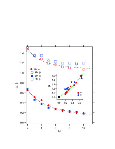
Figure 3: (Color online) The diffusion exponent $\alpha$ and distribution exponent $\beta$ as a function of $M$ for AM and SM. The broken lines are theoretical predictions $\alpha_{M}$ and $\beta_{M}$, respectively. The inset shows the plot of $\beta$ as a function of $\alpha$. The points ($\alpha=0,\beta=1$) and ($\alpha=2/3,\beta=3/2$) are denoted by filled circles which correspond to the exponential localization and subdiffusion at $d=3$, respectively. The green solid curve is the theoretically expected universal relation. The parameters are same to the case of Fig.1 for AM, and $N=2^{14}\sim 2^{16}$, $K=3.1$, $\hbar=\frac{2\pi\times 311}{2^{13}}$ are for SM.

It is found that the numerical results almost agree with the theoretical predictions except for the stretched Gaussian exponent $\beta$ in the perturbed SM with the larger effective dimension $(M+1)\geq 8$. It seems that the disagreement of $\beta$ between the theoretical prediction and numerical data is due to the insufficiency of the ensemble and system size for the tail of the invariant distribution functions.

III Finite-time scaling analysis of the localization-delocalization transitions

We next investigate the critical exponent $\nu$ related to the localization (correlation) length $\xi$, which is supposed to diverge $\xi\sim|\epsilon-\epsilon_{c}|^{-\nu}$ for the localized regime $\epsilon<\epsilon_{c}$ (for the diffusive regime $\epsilon>\epsilon_{c}$). The LDT can be in general observed both for AM and SM. We exhibit here the finite-time scaling analysis for AM taking the case of $M=5$ as the example. First, we show in Fig.4(b) the observed value of $\ln\Lambda(\epsilon,t)$ at various different times $t_{m}$ as a function of $\epsilon$. A remarkable feature is that all the curves crosses at a single point, which can be regarded as $\epsilon_{c}$. This fact allows us to follow the OPST which is usually supposed for the LDT as follows:

$$\Lambda(\epsilon,t) = F((\epsilon_{c}-\epsilon)t^{\alpha/2\nu}),$$ (9)

where $F(x)$ is a differentiable scaling function. We note that the asymptotic function form of $F(x)$ should be $F(x)\to|x|^{-2\nu}$ in order to represent the localization $\Lambda(\epsilon,t)\to t^{{}^{\alpha}}x(\epsilon)\sim t^{{}^{-\alpha}}|\epsilon-\epsilon_{c}|^{-2\nu}$. With the above hypothesis, the scaled MSD can be expressed by $\ln\Lambda(\epsilon,t)-\ln\Lambda_{c}(t)\propto(\epsilon_{c}-\epsilon)t^{\alpha/2\nu}$ around the critical point $\epsilon=\epsilon_{c}$, where $\Lambda_{c}=F(0)$. Applying this relation to the curves in Fig.4(b), we can plot $t_{m}$ and the corresponding slope $s(t_{m})=\ln(\Lambda(\epsilon,t_{m})/\Lambda_{c}(t_{m}))/(\epsilon_{c}-\epsilon)$ , which should $\propto t^{\alpha/2\nu}$, as shown in the inset of Fig.4(a), which enables to decide the unknown exponent $\nu$ by using the known diffusion exponent $\alpha$. With this $\nu$, we can explicitly construct the localization length function $\xi_{s}(\epsilon)=\xi_{0}(\epsilon_{c}-\epsilon)^{-\nu}$ and further the scaling function $F(\xi_{s}(\epsilon)t^{\alpha/2\nu})$ as a function of $x=\xi_{s}(\epsilon)t^{\alpha/2\nu}$. Figure 4(a) shows the scaling functions $F(x)$ constructed by the time-dependent data of MSD at various different $\epsilon$’s close to $\epsilon_{c}$. All the time-dependent data obtained at different $\epsilon$ form a unified function if the scaled variable $x$ is used, which proves numerically the validity of the OPST.

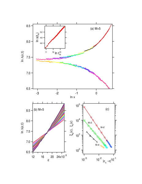
Figure 4: (Color online) The results of the critical scaling analysis for the perturbed AM. (a)The scaled MSD $\Lambda(\epsilon,t)$ as a function of $x=\xi_{s}(\epsilon)t^{\alpha/2\nu}$ for some values of $\epsilon$ in the AM of $M=5$. The $\epsilon$-dependent localization length $\xi_{s}(\epsilon)$ is determined by a scaling relation Eq.(9) by least-square fit in the inset of the panel (a). (b)The same data as panel (a) but plotted as a function of the perturbation strength $\epsilon$. In the ideal case, all lines have a common crossing point at $\epsilon_{c}=0.0175$. (c)The localization length $\xi(\epsilon)$ as a function of $(\epsilon_{c}-\epsilon)$ for $M=2,3,4$. The filled symbols denote the numerical data directly obtained by $\sqrt{m_{2}(t\to\infty)}$ in the long-time limit. The open symbols indicate the localization length $\xi_{s}(\epsilon)$ obtained by OPST in the critical region. Note that the axes are in logarithmic scale.

In Fig.4(c), we compare the localization length function $\xi_{s}(\epsilon)$ decided indirectly by OPST in the critical region $\epsilon\sim\epsilon_{c}$ with $\xi_{n}(\epsilon)$ decided directly by the saturated MSD data which are precisely calculatable for $\epsilon$’s much less than the critical region. The $\epsilon-$dependence of these two localization lengths, $\xi_{s}(\epsilon)$, $\xi_{n}(\epsilon)$, seem to connect continuously, which implies unexpected wideness of the critical region in which the OPST works. Accordingly, Eq.(9) based on the OPST immediately leads to

$$m_{2}(t)\propto(\epsilon-\epsilon_{c})^{-2\nu}x^{2\nu}F(x),$$ (10)

where $x=(\epsilon_{c}-\epsilon)t^{\alpha/2\nu}$ and $F(x)\to x^{-2\nu}$ for $x\to\infty$. It describes the universal relaxation process toward the localized state, but we do not still know to what extent the universal relaxation dynamics works out of the critical region.

IV Critical exponent and perturbation strength of the localization-delocalization transitions

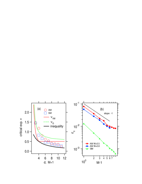
Figure 5: (Color online) (a)The dimensionality $(M+1)=d$ dependence of the critical exponent $\nu$ which characterizes the critical dynamics in the AM and SM. The red solid line and green dashed line are the results of the analytical prediction by $\nu_{VW}$ and $\nu_{G}$, respectively. Thick line denotes the lower bound by the Harris’ critical inequality. (b)The critical perturbation strength $\epsilon_{c}$ as a function of $(M-1)$ for the AM and SM. Note that the axes are in logarithmic scale. Here, we used the SM with $K=3.1$, $\hbar=\frac{2\pi\times 311}{2^{13}}$.

In Fig.5(a), we compare the results of $\nu$ for AM and SM at various $M$ in comparison with theoretical predictions. The critical exponent $\nu$ obtained from the self-consistent mean-field theory of the localization (VW-theory) is $\nu_{VW}=1/(d-2)$ for $2<d<4$ and $\nu_{VW}=1/2$ for $d\geq 4$ vollhard80 . The semiclassical theory of Garcia predicts $\nu_{G}=1/2+1/(d-2)$ which asymptotically approaches the value 1/2 of $\nu_{VW}$ for $d\to\infty$ garcia08b . On the other hand, the inequality $\nu\geq 2/d$ is proposed at the critical point by Harris harris74 . Our results tell that for the larger value of $M(\geq 7)$ the critical exponents of the AM and SM become significantly lower than the theoretical lowest value $1/2$ but satisfy the Harris’ inequality harris74 ; chayes86 ; kramer93 .

Finally, we show the $M$-dependence of the critical strength $\epsilon_{c}$ in Fig.5(b). Note that in the definition of $\epsilon$ we normalized the perturbation by $\sqrt{M}$ in order to make the power strength of perturbation is independent of $M$ for the fixed $\epsilon$. In spite of such a normalization, the critical perturbation strength depends strongly upon $M$. As shown in Fig.5(b), our data for AM and SM indicate the inverse power law

$$\epsilon_{c}\propto(M-1)^{-\delta},$$ (11)

up to $M=10$. The powers are estimated as $\delta\sim 1.1$, for the AM ($W=0.5$ and $0.8$), and $\delta\sim 1.0$ for the SM ($K=3.1$). Eq.(11) means that the total power of the perturbation, which is given by $M\epsilon_{c}^{2}$ is asymptotically proportional to $\sim 1/M$. Such a strong $M-$dependence is highly nontrivial and the theoretical derivation has not been given to the best of our knowledge. It manifests that the LDT with large $M$ is a cooperative phenomenon among the degrees of freedom of perturbation and the driven system.

It is quite interesting that the numerical data of Garcia and Cuevas reporting the delocalization potential threshold of a high-dimensional disordered tight-binding model suggests $(d-2)^{-1}$, which seems to be closely related with our results garcia07 .

V Conclusion

We investigated critical phenomena of LDT exhibited by polychromatically perturbed AM, which models 1DDS perturbed by coherent dynamical perturbations, in comparison with the SM under the same perturbations. We confirmed the presence of critical phenomenon for the mode number $M\geq 2$. The diffusion exponent $\alpha$ and distribution exponent $\beta$ agree well with the theoretical prediction for $M\leq 10$. On the other hand, the critical exponent $\nu$ is significantly lower than the predictions of the mean-field theory for large $M$, but it does not violate the critical inequality. The critical value of normalized perturbation strength exhibits a remarkable $M$-dependence as $\epsilon_{c}\sim(M-1)^{-1}$. As a result, all the critical characteristics of AM agree surprisingly well with SM in spite of their fundamental difference. Our results open a new possibility of controlling electronic localization and conduction by means of externally applied stimulus implemented by optical and/or acoustic devices sheng95 .

References

- (1) K.Ishii, Prog. Theor. Phys. Suppl. 53, 77(1973).
- (2) L.M.Lifshiz, S.A.Gredeskul and L.A.Pastur, Introduction to the theory of Disordered Systems, (Wiley, New York,1988).
- (3) P.Stollmann, Caught by Disorder: Bound States in Random Media, (Birkhauser, 2001).
- (4) E.Abrahams, P.W.Anderson, D.Licciardello, and T.V.Ramakrishnan, Phys. Rev. Lett. 42, 673 (1979).
- (5) A.MacKinnon and B.Kramer, Phys. Rev. Lett. 47, 1546(1981); B.Kramer and A.MacKinnon, Rep. Prog. Phys. 56, 1469(1993).
- (6) K.Slevin and T.Ohtsuki, Phys. Rev. Lett. 78, 4083 (1997).
- (7) A.Croy, P.Cain, and M.Schreiber, Eur. Phys. J. B 82,20212 (2011).
- (8) P. Markos, Acta Phys. Slovaca 56, 561(2006).
- (9) A.M. Garcia-Garcia and E.Cuevas, Phys. Rev. B 75, 174203(2007).
- (10) E. Abrahams (Editor), 50 Years of Anderson Localization, (World Scientific 2010).
- (11) D.R.Grempel, R.E.Prange and S.Fishman, Phys. Rev. A 29,1639(1984); E.Doron and S.Fishman, Phys. Rev. Lett. 60, 867(1988).
- (12) G.Casati, I.Guarneri and D.L.Shepelyansky, Phys. Rev. Lett. 62, 345(1989); F.Borgonovi and D.L.Shepelyansky, Physica D109, 24 (1997).
- (13) K.S.Ikeda, Ann. Phys. 227, 1(1993).
- (14) A.M. Garcia-Garcia, and J.Wang, Phys.Rev.Lett. 100 (2008) 070603.
- (15) C.Tian, A.Altland, and M.Garst, Phys. Rev. Lett. 107, 074101(2011). J.Wang, C.Tian, and A.Altland, Phys. Rev. B 89, 195105(2014).
- (16) J.Chabe, G.Lemarie, B.Gremaud, D.Delande, and P.Szriftgiser, Phys. Rev. Lett. 101, 255702(2008).
- (17) A. Rodriguez, L.J.Vasquez, and R.A.Romer, Phys. Rev. Lett. 102, 106406(2009); G. Lemarie, H.Lignier, D.Delande, P.Szriftgiser, and J.-C.Garreau, Phys. Rev. Lett. 105, 090601(2010); M.Lopez, J.F.Clement, P.Szriftgiser, J.C.Garreau, and D.Delande, Phys. Rev. Lett. 108, 095701(2012).
- (18) H.Yamada and K.S.Ikeda, Phys. Rev. E 59, 5214(1999); ibid, 65, 046211(2002).
- (19) H.Yamada and K.S.Ikeda, Phys. Lett. A 328,170(2004).
- (20) H.S.Yamada and K.S.Ikeda, Eur. Phys. J. B 85,195(2012); ibid 87, 208(2014).
- (21) The frequencies we used are followings: , , , , , , , , , , where denotes the real root of the cubic equation . We have checked for another set of the frequencies. The whole tendency of the main result in the present paper is not depend on the choice for the long-time calculation with large system size.
- (22) A.A. Gogolin, Zh. Eksp. Theor. Fiz. 71 1912(1976), Sov. Phys. JETP 44 1003(1976).
- (23) R.Ketzmerick, K.Kruse, S.Knaut, and T.Geisel, Phys. Rev. Lett. 79 1959(1997); J.Zhong, R.B. Diener, D.A. Steck, W.H. Oskay, M.G. Raizen, E.W. Plummer, Z. Zhang, and Q. Niu, Phys. Rev. Lett. 86, 2485(2001).
- (24) D.Vollhardt, and P. Wolfle, Phys. Rev. Lett. 45,482(1980).
- (25) A.M. Garcia-Garcia, Phys. Rev. Lett. 100, 076404(2008).
- (26) A.B. Harris, J. Phys. C:Solid State Phys. 7, 1671(1974).
- (27) J.T.Chayes, L. Chayes, Daniel S. Fisher, and T. Spencer, Phys. Rev. Lett.57, 2999(1986).
- (28) B.Kramer, Phys. Rev. B47, 9888(1993).
- (29) P. Sheng, Introduction to Wave Scattering, Localization and Mesoscopic Phenomena, (World Scientific, Singapore 1995).