Benchmark Test of Differential Emission Measure Codes and Multi-Thermal Energies in Solar Active Regions

Abstract

We compare the ability of 11 Differential Emission Measure (DEM) forward-fitting and inversion methods to constrain the properties of active regions and solar flares by simulating synthetic data using the instrumental response functions of SDO/AIA, SDO/EVE, RHESSI, and GOES/XRS. The codes include the single-Gaussian DEM, a bi-Gaussian DEM, a fixed-Gaussian DEM, a linear spline DEM, the spatial synthesis DEM, the Monte-Carlo Markov chain DEM, the regularized DEM inversion, the Hinode/XRT method, a polynomial spline DEM, an EVE+GOES, and an EVE+RHESSI method. Averaging the results from all 11 DEM methods, we find the following accuracies in the inversion of physical parameters: the EM-weighted temperature $T_{w}^{fit}/T_{w}^{sim}=0.9\pm 0.1$, the peak emission measure $EM_{p}^{fit}/EM_{p}^{sim}=0.6\pm 0.2$, the total emission measure $EM_{t}^{fit}/EM_{t}^{sim}=0.8\pm 0.3$, and the multi-thermal energies $E_{th}^{fit}/EM_{th}^{sim}=1.2\pm 0.4$. We find that the AIA spatial synthesis, the EVE+GOES, and the EVE+RHESSI method yield the most accurate results.

1 INTRODUCTION

A benchmark test of differential emission measure (DEM) analysis methods is timely since the current capabilities from the Atmospheric Imaging Assembly (AIA; Lemen et al. 2012) and the EUV Variability Experiment (EVE; Woods et al. 2012) onboard the Solar Dynamics Observatory (SDO; Pesnell et al. 2012), combined with simultaneous data from the Reuven Ramaty High Energy Solar Spectroscopic Imager (RHESSI; Lin et al. 2002) and the X-ray Sensor (XRS; Garcia 1994) onboard the Geostationary Operational Environmental Satellite (GOES) series, now offer unprecedented opportunities to design DEM algorithms that take advantage of comprehensive temperature coverage, high spectral resolution, and high spatial resolution in resolving and discriminating complex temperature structures in the solar corona. Another motivation for this study is the calculation of accurate multi-thermal energies, compared with the previously used isothermal approximations, which is the subject of a recent major study on the global energetics of solar flare and coronal mass ejection (CME) events (Aschwanden et al. 2015).

The concept of DEM distributions and the ill-posed problem of the inversion from the observed radiation of optically thin thermal emission (produced by bremsstrahlung [free-free], radiative recombination [free-bound] emission, and even [bound-bound] emission, has been recognized early on (Craig and Brown 1976; Judge, Hubeny, and Brown 1997). It was pointed out that systematic errors resulting from incomplete calculations of atomic excitation levels and from data noise represent a fundamental limitation in DEM inversion (Judge 2010). The inversion of simple synthetic Gaussian or rectangular DEMs was tested with the emission measure loci method, which can retrieve the temperature width of a single-peaked DEM (Landi and Klimchuk 2010). Tests of isothermal DEMs with the Monte Carlo Markov chain (MC) method (Kashyap and Drake 1998), including data noise and uncertainties in the atomic data, revealed that the MC method cannot resolve isothermal plasmas better than $\Delta log(T)\approx 0.05$, and that two isothermal components can not be resolved better than $\Delta log(T)\approx 0.2$ (Landi, Reale, and Testa 2012). Tests on synthetic single-Gaussian and multi-Gaussian DEMs with the regularized inversion technique yielded uncertainties of $\Delta log(T)\approx 0.1-0.5$ and a valid range of the retrieved DEM down to about a level of $\lower 1.72218pt\hbox{$\;\buildrel>\over{\scriptstyle\sim}\;$}1\%$ of the DEM peak emission measure (Hannah and Kontar 2012).

Most of the previously employed DEM methods use spatially-integrated EUV and/or soft X-ray fluxes as constraints, which, for SDO/AIA data, yields typically 6 flux values that are used in the inversion of the DEM function (e.g., Aschwanden and Shimizu 2013). For SDO/EVE, a spatially-integrated spectrometer with $\approx 1$ Å spectral resolution, the data include many tens of spectral lines across hundreds of spectral bins (Warren et al. 2013). However, these EUV-based methods are typically poorly constrained at high temperatures (above $\log(T)~{}\approx 7.3$) due to the relative lack of EUV lines from solar-abundant ions sensitive to these temperatures (e.g., Winebarger et al. 2012). Some more recent DEM methods extend the high-temperature coverage by including GOES/XRS (Warren et al. 2013; Warren 2014) and/or RHESSI (Caspi et al. 2014b; Inglis and Christe 2014) X-ray data, enabling complete coverage of coronal temperatures from $\log(T)~{}\lower 1.72218pt\hbox{$\;\buildrel>\over{\scriptstyle\sim}\;$}6.3$. Fluxes that are spatially integrated over a substantial area of a flare or active region naturally contain many temperatures and thus can have arbitrarily complex broadband DEMs.

A novel method consists of subdividing the observed space into small areas (called macro-pixels or cells), down to the pixel size of the image, which are more likely to encompass a narrower and simpler temperature distribution due to the smaller number of bright structures that are intersected, and then to perform a DEM reconstruction in every macro-pixel, while the total DEM of the entire flare area or active region can then simply be added together. Such a spatial-synthesis method (SS) has been developed for SDO/AIA recently (Aschwanden et al. 2013), and further developments are underway (Cheung et al. 2015).

In this paper we conduct a benchmark test of a set of 11 different DEM forward-fitting and inversion schemes, which include both types of total-flux and spatially-synthesized DEM methods, in order to compare and contrast their accuracy and precision. We perform this test by creating realistic, but synthetic, 2D projected images of flaring loops at all wavelengths using a numerical simulation code; the simulated images are then used to construct spatially-integrated DEMs using the 11 schemes, and are then compared to the true DEM derived from the model input.

2 DATA SIMULATION

2.1 Simulated Differential Emission Measure Maps

We simulate synthetic data of differential emission measure maps $EM(x,y,T)$ as a function of the temperature $T$, in the form of spatial images in the $(x,y)$ plane, sampled in various temperature intervals $[T,T+\Delta T]$ that cover the EUV and soft X-ray wavelength range in a temperature range of $T_{e}=10^{5}-10^{8}$ K. The simulated data aim to mimic loop arcades of large flares with a complex multi-temperature structure.

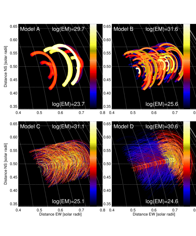
Figure 1.: Simulated total emission measure maps $EM(x,y)$ of the four models: (A) the monolithic scenario with 10 loops with a width of 11 pixels; (B) the intermediate scenario with 100 loops with a width of 5 pixels; (C) the nanoflare scenario with 1000 loops with a width of 1 pixel, and (D) a dual-temperature population model with a width of 1 pixel. The lower and upper limits of $log(EM)$ of the color bar is indicated in each panel. The x-axis and y-axis represents the distance from Sun center in units of solar radii.

The synthetic data cover a $512\times 512$ pixel image with a pixel size of $\Delta x=0.6\hbox{${}^{\prime\prime}$}\approx 435$ km, corresponding to the SDO/AIA pixel scale. The simulated images contain $n_{loop}=$ 10, 100, or 1000 semi-circular flare loops that are randomly distributed along a neutral line, which is centered at a given heliographic location (at longitude $l_{0}=45^{\circ}$ and latitude $b_{0}=30^{\circ}$) and has a length of $L_{0}=200\Delta x\approx 0.125$ solar radii, and is oriented with an azimuthal angle $\alpha=10^{\circ}$ with respect to the East-West direction (x-axis); see an example in Fig. 1. The loops have a half-length that is randomly distributed within a range of $L=(20-200)\Delta x\approx 10-100$ Mm, and have an apex temperature that is randomly distributed within a logarithmic range of $log(T_{max})=6.0-7.3$ K. The temperature profile $T(s)$ along the loops follows the hydrostatic approximation (Aschwanden and Tsiklauri 2009),

$$T(s)=T_{max}\left[\left({s\over L}\right)\left(2-{s\over L}\right)\right]^{2/7}\ ,$$ (1)

with a minimum temperature of $T_{min}=10^{5}$ K at the footpoints. The electron density is uniform along the loop and follows the Rosner-Tucker-Vaiana (RTV) scaling law (Rosner et al. 1978),

$$n_{e}=(8.4\times 10^{5})T_{max}^{2}L^{-1}\ ,$$ (2)

which covers a range of $n_{e}\approx 1.0\times 10^{8}-1.5\times 10^{11}$ cm^-3 here.

We simulate 4 sets of images: Model (A) with a small number of $n=10$ thick loops (with a radius of $r=11$ pixel) that may be typical for spatially resolved monolithic loops (e.g., Aschwanden et al. 2007); Model (B) with a medium number of $n=100$ loops and an intermediate radius of $r=5$ pixels; Model (C) with a large number of $n=1000$ very slender loop strands with a radius of $r=1$ pixel that is typical for unresolved nanoflare loop strands (e.g., Scullion et al. 2014); and Model (D) that contains $n=1000$ loops in two different temperature regimes that form a double-peaked DEM and falls off less steeply at the high-temperature tail of the DEM, while models A, B, and C have a sharp cutoff.

The four models are designed to represent realistic simulations of active regions in the solar corona, regarding spatial structures, temperature distributions, and realistic electron densities as obtained from the RTV scaling law (Rosner et al. 1978). In addition, these four models represent different thermo-spatial patterns, being essentially isothermal in a single pixel with fully resolved loops (Model A), or inherently multi-thermal with spatially unresolved strands (Model C), which cover both extremes (of fully resolved or spatially unresolved temperature structures) to test the capabilities of the different DEM inversion codes. The thermo-spatial pattern matters mostly for pixel-based DEM inversion codes (such as the spatial synthesis code; Section 4.5), while all other codes tested here do not use any spatial information in the DEM inversion. Therefore, we will learn whether or not the inclusion of spatial information affects the accuracy of DEM reconstructions. One new DEM inversion code that uses spatial information also has been designed recently (Cheung et al. 2015).

Each individual loop is uniformly filled with space-filling voxels $(x,y,z)$ that have a volume $(\Delta x)^{3}$, a unique electron temperature $T(x,y,z)$, and electron density $n_{e}(x,y,z)$. The pixelized data cube $EM(x,y,z,T)$ is then integrated along the line-of-sight in direction of the z-axis in order to produce differential emission measure maps in each temperature interval,

$$EM(x,y,T)=\int n_{e}^{2}(x,y,z,T)dz\ ,$$ (3)

which has the units of [cm^-5 K^-1]. Simulated total emission measure maps, integrated over the temperature range $T$ with units of [cm^-5],

$$EM(x,y)=\int EM(x,y,T)dT\ ,$$ (4)

are shown for all 4 cases in Fig. 1. The temperature is discretized in a logarithmic range of $log(T_{e})=5.00,5.05,...,8.00$ in 61 equidistant logarithmic steps with a width of $\Delta log(T)=0.05$ each. A total differential emission measure distribution $EM_{tot}$ integrated over the entire volume is defined by

$$EM_{tot}(T)=\int\int EM(x,y,T)\ dxdy\ ,$$ (5)

and has the units of [cm^-3 K^-1].

2.2 Simulation of AIA Flux Maps

The differential emission measure maps $EM(x,y,T)$ are defined in an instrument -independent way. In order to simulate observables, the simulated theoretical differential emission measure $EM(x,y,T)$ is then convolved with the instrumental response function $R_{\lambda}(T)$ (in units of [DN s^-1 cm⁵] per pixel) of a particular temperature filter, in order to obtain the expected flux maps $f_{\lambda}(x,y)$ (in units of DN/s),

$$f_{\lambda}(x,y)=\int EM(x,y,T)\ R_{\lambda}(T)\ dT=\sum_{k=1}^{n_{T}}EM(x,y,T_{k})\ R_{\lambda}(T_{k})\Delta T_{k}\ ,$$ (6)

where $n_{T}$ is the number of temperature filters, and $f_{\lambda}$ are the observed fluxes in the coronally-domainted EUV wavelengths $\lambda$ = 94, 131, 171, 193, 211, 335 Å, in the case of the SDO/AIA instrument. For the temperature integration we are using the discretized temperature intervals $\Delta log(T_{k})$, which are chosen in equidistant bins with a width of $\Delta log(T_{k})=log(T_{k+1})-log(T_{k})=0.05$. This way we obtain 6 simulated AIA images for which the differential emission measure distribution $EM(x,y,T)$ is exactly known from the theoretical model. We can then use these flux maps $f_{\lambda}(x,y)$, $\lambda=1,...,6$ to test the various DEM inversion codes and methods. An example of 6 simulated AIA flux maps is shown in Fig. 2 (Model B).

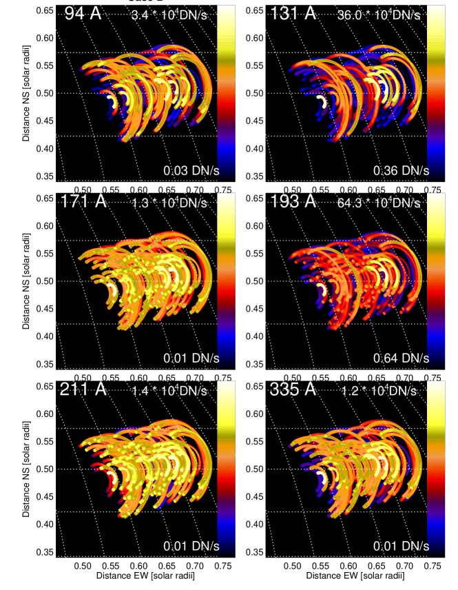
Figure 2.: Simulated AIA flux maps $F_{\lambda}(x,y)$ for the 6 AIA wavelengths. The simulation of model B includes 100 flare loops with a width of 5 pixels in a temperature range of $T_{e}=1-20$ MK. The lower and upper flux limits of the color bar are indicated in each panel. The x-axis and y-axis represents the distance from Sun center in units of solar radii.

2.3 Multi-Thermal Energy

The multi-thermal energy, which is the integral of all thermal energies integrated over each temperature range $\Delta T_{k}$, is defined as

$$E_{th}=\sum_{k}3k_{B}V^{1/2}\ T_{k}\ EM_{k}^{1/2}\ .$$ (7)

This expression can substantially deviate from the isothermal approximation (independent of the DEM inversion method),

$$E_{th,iso}=3n_{p}k_{B}T_{p}V=3k_{B}T_{p}\sqrt{EM_{p}\ V}\ ,$$ (8)

which assumes a narrow delta-like DEM distribution that can be characterized by the DEM peak temperature $T_{p}$ and DEM peak emission measure $EM_{p}$. Separate calculations of isothermal and multi-thermal energies based on the same DEM fitting method in $\approx 400$ M- and X-class flares has shown that the multi-thermal energy exceeds the isothermal energy by a factor of $\sim 14$ in the statistical average (Aschwanden et al. 2015). A comparison with these multi-thermal energies shows that our 4 models have conditions that are typical for active regions, rather than for large flares.

3 INSTRUMENTAL RESPONSE FUNCTIONS

3.1 The SDO/AIA Response Functions

The AIA instrument onboard SDO started observations on 29 March 2010 and has produced since then essentially continuous data of the full Sun with four $4096\times 4096$ detectors with a pixel scale of $0.6\hbox{${}^{\prime\prime}$}$, corresponding to an effective spatial resolution of $\approx 1.5\hbox{${}^{\prime\prime}$}$ (Lemen et al. 2012). AIA contains ten different wavelength channels, three in white light and UV, and seven EUV channels, of which six wavelengths (131, 171, 193, 211, 335, 94 Å) are centered on strong iron lines (Fe viii, ix, xii, xiv, xvi, xviii), covering the coronal range from $T\approx 0.6$ MK to $\lower 1.72218pt\hbox{$\;\buildrel>\over{\scriptstyle\sim}\;$}16$ MK. AIA records a full set of near-simultaneous images in each temperature filter with a fixed cadence of 12 s. Instrumental descriptions can be found in Lemen et al. (2012) and Boerner et al. (2012, 2014). The nominal AIA response functions $R_{\lambda}(T)$ are shown in Fig. 3. We use the currently available calibration, which was updated with improved atomic emissivities according to the CHIANTI Version 7 code, distributed in the Solar SoftWare (SSW) on 2012 February 13. Although the response functions of the AIA channels (with a full width of $\log{(\Delta T)}\approx 0.2$) are relatively narrowband (compared with GOES or Yohkoh/SXT), we have to be aware that this intrinsic temperature width represents an ultimate lower limit for resolving multiple temperature structures, and thus constitutes a bias in the inversion of narrrower (more isothermal) temperature structures in the DEM inversion, as previously verified (e.g., Kashyap and Drake 1998; Landi et al., 2012). An additional caveat of widely distributed DEMs is that the intensity is completely smoothed out, regardless of the shape of the response function. Although AIA has the ability to reconstruct simple DEM forms, the greater the width of the plasma DEM is, the lower is the accuracy and precision in the determination of the DEM parameters, which is a fundamental limitation (Guennou et al. 2012).

Another uncertainty in DEM reconstructions comes from atomic physics, such as the atomic line emissivities, the assumption of ionization equilibrium, and variations in elemental abundances between the chromosphere and corona. The AIA response functions were calculated based on the latest version (7.1) of the CHIANTI code. While the line intensities in the wavelength range of 170–350 Å included in CHIANTI are considered to be satisfactory, the CHIANTI Version 7.1 code appears to underpredict the observed intensities in the 50–150 Å wavelength range by factors of 2-6 (Boerner et al. 2014), which affects mostly the 94 and 131 Å channels (Aschwanden and Boerner 2011; Teriaca, Warren, and Curdt, 2012), a fact that was also corroborated with measurements of spectra from the star Procyon taken by Chandra’s LETG (Testa, Drake, and Landi 2012b). Regarding elemental abundance variations, AIA has been designed to consist of 6 coronal wavelength channels that are all sensitive to iron lines, and thus the elemental abundance of iron, which exhibits the largest first-ionization potential (FIP) effect, largely cancels out in the combination of the six coronal AIA channels. However, although the shape of the reconstructed DEM is not much affected when only iron lines are used, the magnitude of the DEM still depends on the absolutie value of the iron abundance, which may have a substantially larger error than 10%. In our benchmark study we choose to neglect the atomic physics uncertainties, which makes the expected cancellation of the FIP effect less certain.

The calibration uncertainties of the AIA response function have been estimated to be 25% in absolute terms, using a comparison of full-disk-integrated fluxes with SDO/EVE, but reduce to $\lower 1.72218pt\hbox{$\;\buildrel<\over{\scriptstyle\sim}\;$}10\%$ after application of the cross-calibration (Boerner et al. 2014). The residual ratios left from fitting the AIA /EVE flux ratios are shown in Fig. 2 of Boerner et al. (2014) and can also be obtained from the IDL Solar SoftWare (SSW) procedure aia$\_$bp$\_$read$\_$error$\_$table. The individual uncertainties in the different AIA channels amount to: 8.7% ( 94 Å), 5.1% (131 Å), 1.9% (171 Å), 1.4% (193 Å), 1.9% (211 Å), 2.3% (304 Å), 9.7% (335 Å), so we conservatively adopt 10% as an upper limit.

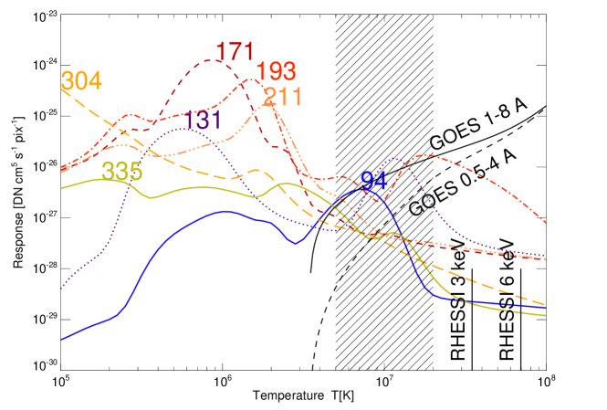
Figure 3.: Temperature-response functions for the seven coronal EUV channels of the Atmospheric Imaging Assembly (AIA) onboard the Solar Dynamics Observatory (SDO), according to the status of Dec 2012. The GOES/XRS 1-8 Å and 0.5-4 Å response is also shown (in arbitrary flux units), as well as the thermal energy of the lowest fittable RHESSI channels at 3 keV and 6 keV. The approximate peak temperature range of large flares ($T_{p}\approx 5-20$ MK) is indicated with a hatched area.

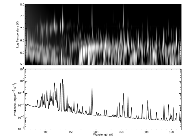
Figure 4.: The SDO/EVE response function $R_{EVE}(\lambda,T)$, represented here as the CHIANTI emissivity convolved with the EVE spectral resolution, as a function of the wavelength $\lambda$ (horizontal axis) and temperature (vertical axis in top panel), in the range of $\lambda=60-350$ Å and $log(T_{e})=5.5-8.0$. (bottom panel) An isothermal spectrum at a temperature of $log(T_{e})=7.1$ and an emission measure of $10^{51}$ cm³ is shown. The temperature is indicated by a dotted line in the upper panel).

3.2 The SDO/EVE Response Function

The EVE onboard SDO measures the solar irradiance at many EUV wavelengths. Here we use observations from the Multiple EUV Grating Spectrograph A (MEGS-A), a grazing incidence spectrograph that operates in the 50-370 Å wavelength range, has a spectral resolution of $\sim 1$ Å, and an observing cadence of 10 s. The observed emission at these wavelengths is sensitive to temperatures ranging from the upper chromosphere (He II 304 Å) to about 25 MK (Fe XXIV 192 and 255 Å). Since the peak temperature sensitivity of the MEGS-A is below the peak temperature observed in many flares, it is useful to combine EVE observations with observations from other instruments that are sensitive to higher temperature emission (e.g., GOES/XRS, RHESSI).

The modest spectral resolution of the MEGS-A means that while many spectral features can be easily identified, many are blended and reliably calculating the fluxes of individual emission lines is difficult. Our strategy is to compute theoretical spectra from CHIANTI, convolve them with the EVE spectral resolution, and to compare these spectra directly with the observations in selected wavelength ranges. The calculated spectra used for this work are shown in Figure 4. Further details are given in Warren et al. (2013) and Caspi et al. (2014b).

We note that since the spectral information is preserved in the treatment of the EVE observations, the application of random perturbations affects these data differently than other broadband measurements. For the broadband measurements the integrated intensity is perturbed. With the EVE data we are perturbing the intensity in each spectral pixel and thus the fluctuations tend to average out, leaving the intensity in each spectral feature largely unchanged. A more realistic treatment would be to smoothly vary the effective areas that are used to convert the observed count rates to absolute intensities. Our expectation is that the uncertainty in the calibration is dominated by systematic trends and not pixel-to-pixel noise. Such a procedure would be relatively easy to implement, but is beyond the scope of this work.

One subtlety of analyzing the actual EVE observations is that unidentified emission lines make significant contributions to some wavelength ranges and the calculated spectra cannot be matched to the observations in these regions (Warren 2005; Testa et al. 2012b). This can be addressed by subtracting a pre-flare spectrum from the observed spectra during the flare (e.g., Warren et al. 2013; Caspi et al. 2014b). For this work, which considers theoretical spectra, we do not apply background subtraction since no background is simulated in the synthesized input.

3.3 The RHESSI Response Function

RHESSI observes solar photons from $\sim$ 3 keV to $\sim$ 17 MeV (Lin et al. 2002), using a set of nine cryogenically cooled coaxial germanium detectors to achieve $\;\buildrel<\over{\scriptstyle\sim}\;$1 keV FWHM spectral resolution (Smith et al. 2002). RHESSI is also capable of imaging X-ray and gamma-ray sources through a Fourier method (Hurford et al. 2002), but we do not use the imaging capabilities for this work.

Since flare temperatures of $T_{e}\approx 5-50$ MK correspond to thermal electron energies of $E_{th}=k_{B}T_{e}\approx 0.4-4.4$ keV (Fig. 3), RHESSI is sensitive to the high-temperature tails of flare DEMs, whose emission typically dominates the RHESSI spectrum in the $3-20$ keV energy range. While most of the thermal emission detected in this range is produced by the free-free (bremsstrahlung) and free-bound (radiative recombination) continuum processes, RHESSI also observes the line emission of two iron-dominated line complexes at $\sim 6.7$ (Fe) and $\sim 8$ (Fe/Ni) keV (Phillips 2004; Phillips et al. 2006; Phillips 2008; Caspi and Lin 2010).

When multiple thermal components are present, fitting of RHESSI thermal spectra in isolation has a bias towards higher temperatures because of RHESSI’s exponentially-increasing temperature sensitivity (McTiernan 2009). For intense flares where the DEM tail extends to very high temperatures, an isothermal or delta-function DEM analysis often yields a “super-hot” component in the temperature range of $T_{e}\approx 20-50$ MK (e.g., Caspi and Lin 2010; Caspi et al. 2014a), which is significantly higher than the DEM peak temperature (with a typical range of $T_{e}\approx 10-20$ MK), a bias that was also quantitatively investigated in Ryan et al. (2014). Improved temperature diagnostics can be obtained by combining RHESSI high-temperature spectra with the broadband EVE irradiance spectra that are sensitive to the lower-temperature emission, a method that has been successfully applied to two X-class flare events so far (Caspi et al. 2014b).

3.4 The GOES Response Function

The GOES X-Ray Sensor (XRS) measures spatially integrated broadband solar X-ray radiation in two overlapping passbands: 1-8 Å and 0.5-4 Å. In typical solar conditions, it is most sensitive to coronal emission from temperatures of $\sim 4-40$ MK. This is ideal for examining the bulk thermal emission of M- and X-class flares which have typical peak temperatures of $10-25$ MK (Ryan et al. 2012). The XRS detectors comprise two ion chambers, one for each channel. The output currents of the ion chambers are related to the incident X-ray flux via wavelength-dependent transfer functions (Garcia 1994; Hanser and Sellers 1996). The GOES/XRS response function is calculated based on the CHIANTI code assuming photospheric (or coronal) elemental abundances and ionization equilibrium (e.g. Feldman et al. 1992; Mazzotta et al. 1998). Normally when analyzing GOES/XRS observations, the DEM is assumed to be isothermal and is then derived from the ratio of the short and long channel fluxes (Thomas et al. 1985; Garcia 1994; White et al. 2005). This limitation is given because the two-channel data can only constrain a single temperature with a filter-ratio technique. The isothermal approximation, however, has a temperature bias for multi-thermal DEM distributions (see Eq. (7) in Ryan et al. 2014). The two-channel data alone also cannot strongly constrain broad DEM solutions of forward-fitting techniques, resulting in a wide range of non-unique solutions. Combining GOES/XRS with other instruments, however, such as with SDO/EVE (Warren et al. 2013) as used in this work, provides the necessary constraints to yield more realistic multi-thermal DEMs.

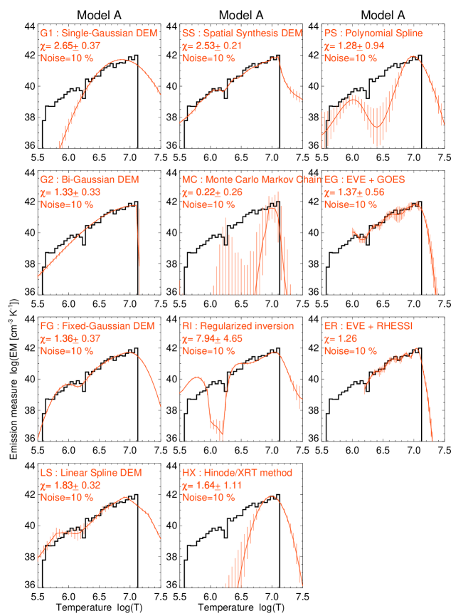
Figure 5.: DEM inversions of monolithic loop model A, using 11 different DEM forward-fitting or inversion methods. The simulated DEM is indicated with a black histogram, while the average of 30 DEM inversions (by adding 10% noise to the simulated fluxes) are indicated with red curves, including error bars. The reduced $\chi^{2}$ is computed from the average of the 30 runs. The x-axis represents the logarithm of the temperature in units of K.

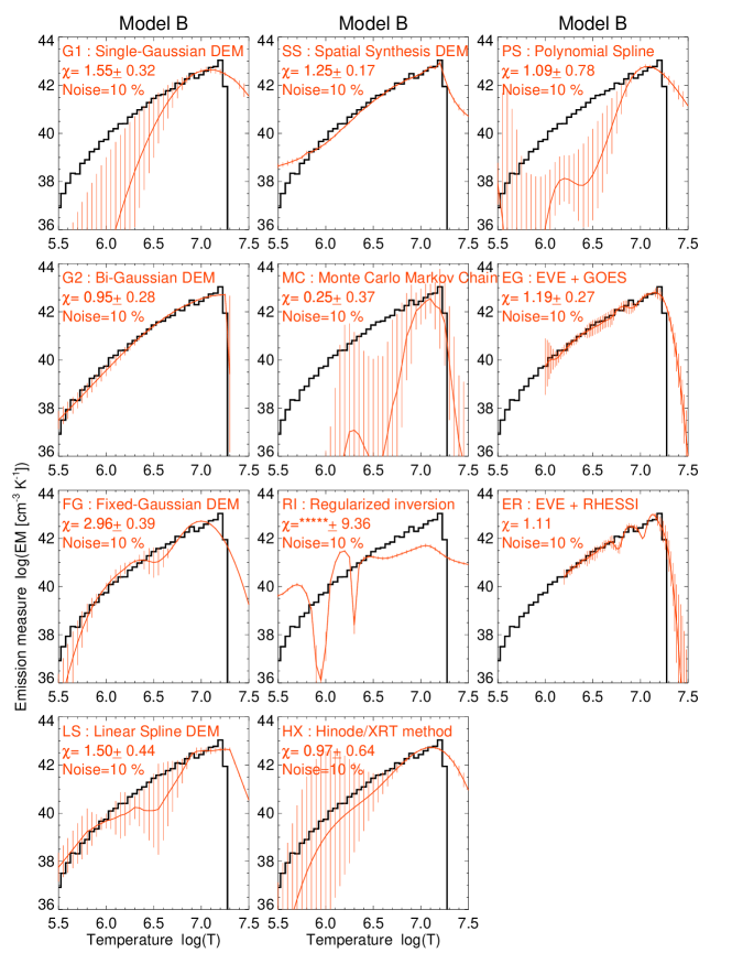
Figure 6.: DEM inversions for thin loop model B, using 11 different DEM methods. Otherwise representation similar to Fig. 5.

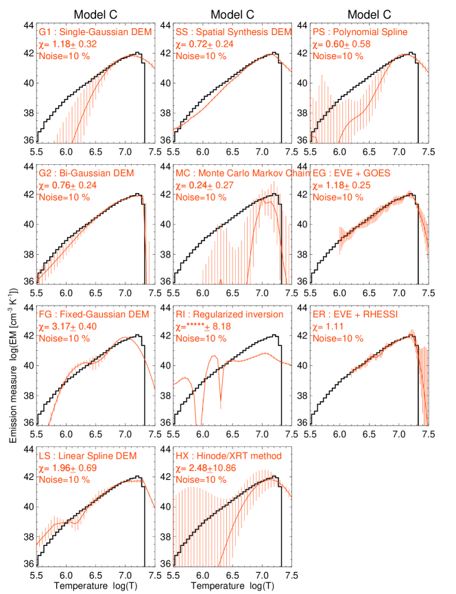
Figure 7.: DEM inversions for nanoflare loop model C, using 11 different DEM methods. Otherwise representation similar to Fig. 5.

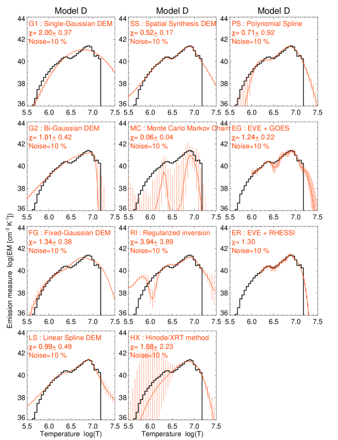
Figure 8.: DEM inversions for the dual-temperature arcade model D, using 11 different DEM methods. Otherwise representation similar to Fig. 5.

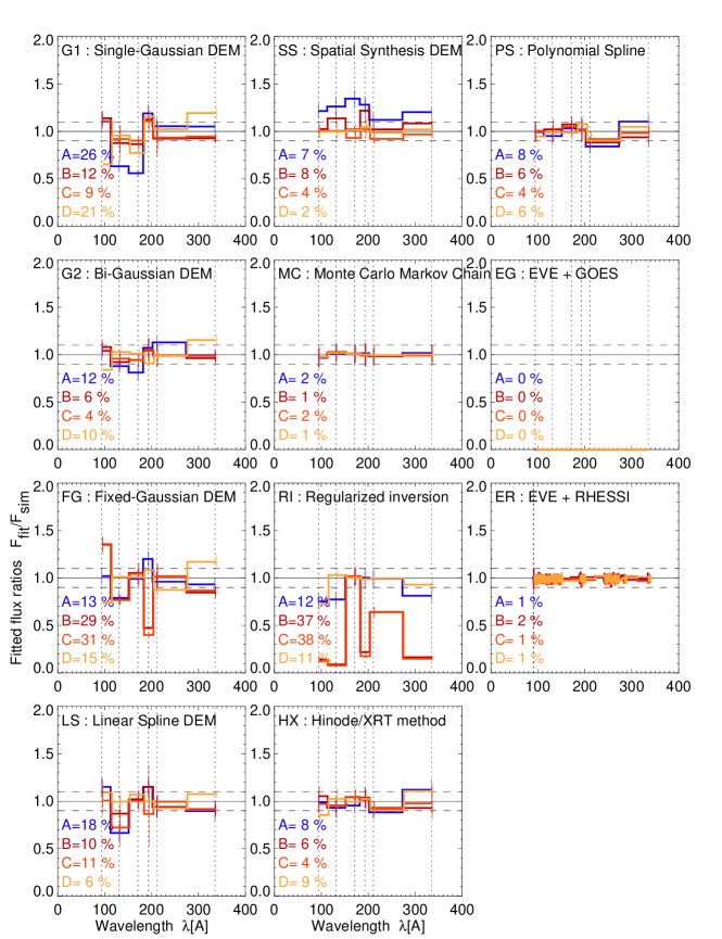
Figure 9.: Ratios of fitted fluxes to simulated fluxes for the 6 AIA wavelengths. The error bars were obtained from adding 10% random noise to the simulated fluxes. The standard deviation of the fitted to the simulated fluxes are quoted in percentages. The x-axis represents the logarithm of the temperature in units of K.

Figure 10.: The accuracy of the 11 DEM inversion methods is shown by the ratio of the best-fit and simulated emission measure, $\log(EM^{fit}/EM^{sim})$, as a function of the temperature $\log(T)$, where the color indicates the three simulations A (blue), B (brown), C (red), and D (orange). The ranges within two orders of magnitude below the peak emission measure $EM^{sim}$ are indicated with dotted vertical lines and the average deviations in percentages are listed for this range. The x-axis represents the temperature in units of K.

Table 1.: Characteristics of 11 DEM methods applied in this study: Name of DEM method, DEM parameterization function, degrees of freedom, optimization algorithm, number of spatial pixels, and instrument of used data.

Method	Parametrization	Degrees	Optimization	Pixels	Data
		of	algorithm
		freedom
G1	Single Gaussian	3	Least-square minimization	1	AIA
G2	Bi-Gaussian	4	Least-square minimization	1	AIA
FG	Fixed Gaussians	4-6	Least-square minimization	1	AIA
LS	Linear Spline	4-6	Least-square minimization	1	AIA
SS	Single Gaussian	3	Least-square minimization	16,384	AIA
MC	N/A	61	Markov chain Monte Carlo	1	AIA
RI	N/A	61	Regularized Inversion	1	AIA
HX	Spline	4-6	Least-square minimization	1	AIA
PS	Spline	4-6	Least-square minimization	1	AIA
EG	Fixed Gaussians	10-20	Least-square minimization	1	EVE+
					GOES
ER	Fixed Gaussians	10-20	Least-square minimization	1	EVE+
					RHESSI

4 DEM INVERSION METHODS AND RESULTS

In the following section, we describe 11 different DEM inversion and forward-fitting methods, where each method consists of a choice of DEM parameterization, degrees of freedom, optimization algorithm, spatial summing, and data set from different instruments, as indicated in Table 1 for the cases studied here. In the following we present also the results that these 11 methods produce for the 4 simulated models A-D pictured in Fig. (1). The results are graphically presented in Figs. (5-10), and quantitatively compiled in Tables 2 and 3.

The values of the simulated DEM peak temperature $T_{p}$, the DEM peak emission measure $EM_{p}$, the total emission measure $EM_{tot}$, the multi-thermal energy $E_{th}$, and the $\chi^{2}$-values of the best fits are specified in Table 2 for the 4 models (A-D), while the ratios of the best-fit values to the simulated values are compiled in Table 3. The ratios of the fitted to the simulated wavelength fluxes are graphically presented in Fig. (9), while the (logarithmic) ratios of the simulated to the inverted DEMs are shown in Fig. (10).

4.1 Single-Gaussian DEM Fit (G1)

One of the most robust choices of a DEM function with a minimum of free parameters is a single Gaussian (in the logarithm of the temperature), which has 3 free parameters only and is defined by the peak emission measure $EM_{p}$, the DEM peak temperature $T_{p}$, and the logarithmic Gaussian temperature width $w$. The DEM parameter has the cgs-units [cm^-5 K^-1],

$$EM(T)=n_{e}^{2}{dz\over dT}=EM_{p}\exp{\left(-{[log(T)-log(T_{p})]^{2}\over 2w^{2}}\right)}\ ,$$ (9)

where the total emission measure $EM=n_{e}^{2}dz=\int EM(T)\ dT$ is the temperature integral over the Gaussian DEM (in units of [cm^-5]). Single-Gaussian DEM fits have been used in many studies with AIA data (e.g., Aschwanden and Boerner 2011; Aschwanden and Shimizu 2013; Ryan et al. 2014).

In our DEM forward-fitting code we define logarithmically-spaced values for the electron temperature, $log(T_{p})=5.0,...,8.0$ K, for the logarithmic Gaussian width $w=0.01,...,1$, and for the peak emission measure values $log(EM_{p})=23,...,29$. The temperature range is identical to the discretized definition of the instrumental response function $R(T)$. Approximate best-fit values are then found simply by a global search in this 3-parameter space $[T_{p},w,EM_{p}]$ by calculating the minimum of the reduced $\chi^{2}$-criterion (e.g., Bevington and Robinson 1992),

$$\chi^{2}_{red}=\left[{1\over n_{free}}\sum_{\lambda=1}^{n_{\lambda}}{(f_{\lambda}^{fit}-f_{\lambda}^{sim})^{2}\over\sigma_{\lambda}^{2}}\right]^{1/2}\ ,$$ (10)

where $f_{\lambda}^{sim}$ are the 6 simulated AIA flux values, $f_{\lambda}^{fit}$ are the fitted flux values (using the Gaussian EM(T) defined in Eq. 9),

$$f_{\lambda}(T_{p},w,EM_{p})=\sum_{k=1}^{n_{T}}EM(T_{k},w,EM)\ R_{\lambda}(T_{k})\ \Delta T_{k}\ ,$$ (11)

$\sigma_{\lambda}$ are the estimated uncertainties, $n_{free}=n_{\lambda}-n_{par}$ is the number of degrees of freedom, which is $n_{free}=3$ for $n_{\lambda}=6$, the number of AIA wavelength filters, and $n_{par}=3$, the number of model parameters. The uncertainties $\sigma_{\lambda}$, which are dominated by the inaccuracies in the knowledge of the AIA instrumental response function, are estimated to be of the order of 10% of the observed fluxes (Boerner et al. 2014). We neglect the Poisson noise of the photon statistics, which is on the order of $\sqrt{(N)}/N\approx 10^{-4}-10^{-3}$ for AIA count rates of $N\approx 10^{6}-10^{8}$ photons/s (Boerner et al. 2014; O’Dwyer et al. 2010). Consequently, the estimate of the uncertainty is

$$\sigma_{\lambda}\approx q_{noise}\ f_{\lambda}^{sim}\ ,$$ (12)

with $q_{noise}\approx 0.1$. We generate simulated fluxes by adding 10% random noise to the noise-free data, i.e., $f_{\lambda}^{ran}=(1+\rho_{\lambda}\ q_{noise})\ f_{\lambda}^{sim}$, where random values $\rho_{\lambda}$ are drawn from a normal distribution with a standard deviation of unity. From a global search of the minimum in the 3-parameter space $[T_{p},w,EM_{p}]$ we obtain an approximate solution for the DEM, which we use as initial guess for a refined optimization using the Powell $\chi^{2}$-minimization method (Press et al. 1986).

Results G1: We turn now to the results of our DEM fits. The best fits to the simulated fluxes $f_{\lambda}^{sim}$ (Eq. 6) of a single-Gaussian DEM function are shown in Figures 5-8 (top left panel), which fit the simulated DEM function most accurately near the peak of the DEM, but yield too low DEM values at the low-temperature side and too high DEM values at the high-temperature side. We see that the model-predicted fitted flux values differ by 9%-26% with respect to the simulated input flux values for the four cases A-D (Fig. 9), and the resulting DEM functions differs by 13%-19% (Fig. 10). Obviously, a single-Gaussian DEM function cannot fit a highly asymmetric DEM well, but is likely to do better for a near-symmetric single-peaked DEM distribution function. This is also consistent with the goodness-of-fit criterion, which yields values significantly above unity for all 4 cases A-D (Fig. 5-8), indicating that the G1 model does not fit the data as well as possible within the estimated flux uncertainties.

4.2 Bi-Gaussian DEM Fit (G2)

In order to accommodate asymmetric DEM functions, we introduce the bi-Gaussian DEM function (G2), which is composed of two semi-Gaussian functions with two different temperature half widths $w_{1}$ and $w_{2}$ on the left and right side,

$$EM(T)=EM_{p}\exp{\left(-{[log(T)-log(T_{p})]^{2}\over 2\ w^{2}}\right)}\quad\left\{\begin{array}[]{ll}w=w_{1}&{\rm for}\ T\leq T_{p}\\ w=w_{2}&{\rm for}\ T\geq T_{p}\\ \end{array}\right.\ ,$$ (13)

with a total of four variables ($n_{par}$), i.e., $EM_{p},T_{p},w_{1},w_{2}$. Since the AIA instrument has $n_{par}=6$ coronal wavelength filters, there are two degrees of freedom, $n_{free}=n_{\lambda}-n_{par}=6-4=2$, for this model.

We choose equidistant values in the logarithmic ranges of $log(EM_{p})=23,...,$ 29 for the emission measure (cm^-5 K^-1), $log(T_{p})=5.5,...,7.5$ for the peak temperatures (K), and $w=0.01,...,10$ for the Gaussian widths. As with the single-Gaussian method, G1, we find first an approximate DEM solution from an absolute search in the discretized three-dimensional parameter space, which is then used as initial guess for subsequent optimization with the Powell $\chi^{2}$-minimization method (Press et al. 1986).

Results G2: The best fits are shown in Figs. (5)-(10) (second left panels). All of the fits for the four models A-D represent the peak of the asymmetric DEM function better than the (symmetric) single-Gaussian fits from G1. The low-temperature side of the DEM function can be fitted with a large semi-Gaussian width of $w1\approx 1.5$ and the high-temperature side with a very small semi-Gaussian width of $w_{2}\approx 0.01$ to mimic the steep drop-off. The goodness-of-fit criterion varies in the range of $\chi^{2}\approx 0.76-1.33$ for the four cases A-D (Figs. 5-8; second left frames), the fitted flux values differ by 4%-12% with respect to the simulated flux values (Fig. 9), and the resulting DEM functions differ by 11%-15% (Fig. 10). The actual uncertainty of the AIA response function is comparable, i.e., $\sim 10\%$ (Boerner et al. 2014), which we emulate here by generating 30 data sets of fluxes with 10% noise added. The bi-Gaussian DEM function turns out to be a good choice for the asymmetric single-peaked DEM models A-C used here, but is by nature less adequate to fit multi-peaked DEMs (such as model D).

4.3 Multiple Fixed-Gaussian DEM Fit (FG)

In principle, one can define a more versatile DEM function by a superposition of an arbitrary number of Gaussian functions (Eq. 9, $n>2$), but the number of free parameters will increase by $n_{free}=3n$, which becomes prohibitive for practical purposes of numerical fitting. One way to keep the number of free parameters within a reasonable limit is to fix the peak temperatures $T_{p,i}$ at logarithmically equi-spaced values (with a step of $\Delta log(T)$) and to fix the Gaussian widths to a value that corresponds to about half the separation step, i.e., $w=\Delta log(T)/2$, so that only the emission measure values $EM_{p,i}$ have to be optimized. Such a multiple fixed-Gaussian method (FG) has been applied in several studies using AIA or EVE data (e.g., Aschwanden and Boerner 2011; Warren et al. 2013; Caspi et al. 2014b; Warren 2014). In this section, we apply this method to the AIA data alone; the application to combined EUV and X-ray data, using EVE and GOES/XRS and/or RHESSI together, is discussed in later sections.

Results FG: We show the application of such a multiple fixed-Gaussian DEM method to the three models A, B, and C in Figs. (5-10) (third left panel), using six fixed Gaussians centered at the temperatures $log(T)$=6.00, 6.25, …, 7.25 with a fixed width of $w=0.13$. The best fits show a double-humped DEM function, which seem to depend somewhat on the choice of the fixed temperatures $T_{p,i}$. In any case, the DEM function with fixed Gaussians appears to fit the examples here with less accuracy than the bi-Gaussian function. The goodness-of-fit criterion varies in the range of $\chi^{2}\approx 1.4-3.2$ for the four cases A-D (Figs. (5-8), third left frames), the fitted flux values differ by 13%-31% with respect to the simulated flux values (Fig. 9), and the resulting DEM functions differ by 11%-18% (Fig. 10). We conclude that DEM functions with multiple fixed Gaussians can provide good fits when the fixed temperatures agree with the peaks of the DEM, which requires some fiddling of the fixed peak temperature values. However, we note that the application of this method with EVE+GOES and EVE+RHESSI data yields superior fits (see below), most likely because of the significantly greater EUV spectral data available from EVE, combined with the strong constraints on the high-temperature tail provided by the X-ray data, which also allow a greater number of fixed Gaussian components to be used in the model.

4.4 Linear Spline DEM Fit (LS)

Spline functions are defined by fixed points $x_{i}$ on the x-axis, which have some particular values $y_{i}=y(x_{i})$ on the y-axis, and are linearly interpolated in between. We choose 5 temperature spline points $T_{k},k=1,...,5$ on the logarithmic x-axis covering the range of $T_{k}=10^{5.8},...,10^{7.3}$ K, and consider the corresponding 5 spline values $EM_{k},k=1,...,5$ as free parameters to be fitted, which is very similar to the multiple fixed-Gaussian fitting method. The spline points have a fixed step of $\Delta log(T_{k})=0.375$. We find an initial guess with an absolute minimum search in the five-dimensional $\chi^{2}$-space, followed by subsequent Powell optimization.

Results LS: We show the application of such a linear spline DEM fitting method to the four models A-D (Figs. 5-8), The goodness-of-fit criterion varies in the range of $\chi^{2}\approx 1.5-2.0$ for the 4 cases (Figs. (5-8), the fitted flux values differ by 6%-18% with respect to the simulated flux values (Fig. 9), and the resulting DEM functions differ by 12%-46% (Fig. 10). In conclusion, the linear spline function fits the simulated DEMs with similar accuracy as the multiple fixed-Gaussian method, but not as good as the bi-Gaussian function in these particular simulations. However, for the general case with multiple DEM peaks, the linear spline function is expected to be more flexible than a single-Gaussian or bi-Gaussian function.

4.5 Spatial Synthesis DEM Method (SS)

The DEM methods used so far all use the total spatially-integrated flux from an observed area that corresponds to the flare or active region size, and thus contains many locations with possibly quite different temperature structures. Applying a DEM inversion to a single pixel of an image, we are more likely to disentangle the complex multi-temperature structures into simpler components, in some cases as simple as a near-isothermal segment of a resolved monolithic loop, in which case a Gaussian fit becomes more adequate.

A sensible approach to the temperature discrimination problem is to subdivide the image area of a flare into macro-pixels or even single pixels, and then to perform a forward-fit of a single-Gaussian DEM function in each spatial location separately, while the total DEM distribution function of the entire flare area can then be constructed by summing all DEM functions from each spatial location, which we call the “Spatial Synthesis DEM” method. This way, the Gaussian approximation of a DEM function is applied locally only, but can adjust to different peak emission measures and temperatures at each spatial location. Such a macro-pixel algorithm for automated temperature and emission measure analysis has been developed for AIA wavelength-filter images in Aschwanden et al. (2013), and a SSW/IDL code is available online (http://www.lmsal.com/$\sim$aschwand/ software/aia/aia$\_$dem.html). The flux $F_{\lambda}(x,y,t)$ is then measured in each macro-pixel location $[x,y]$ and the fitted DEM functions are defined at each location $[x,y]$ separately,

$$EM(x,y;T)=EM_{p}(x,y)\exp{\left(-{[log(T)-log(T_{p}[x,y])]^{2}\over 2\ w^{2}[x,y]}\right)}\ ,$$ (14)

and are forward-fitted to the observed fluxes $F_{\lambda}(x,y)$ at each location $(x,y)$ separately, after background subtraction of $B_{\lambda}(x_{i},y_{j})$ (which is set to zero in our simulated cases here),

$$F_{\lambda}(x_{i},y_{j})-B_{\lambda}(x_{i},y_{j})=\sum_{k=1}^{n_{T}}EM(x_{i},y_{j};T_{k})R_{\lambda}(T_{k})\ .$$ (15)

The synthesized differential emission measure distribution $EM(T)$ can then be obtained by summing up all local DEM distribution functions $EM(T;x,y,t)$ (in units of cm^-3 K^-1),

$$EM(T)=\sum_{i}\sum_{j}EM(x_{i},y_{j};T_{k})\ dx_{i}dy_{j}\ ,$$ (16)

and the total emission measure of a flaring region is then obtained by integration over the temperature range (in units of cm^-3),

$$EM=\sum_{k}EM_{k}(T_{k})\ \Delta T_{k}\ .$$ (17)

Note that the synthesized DEM function $EM(T)$ (Eq. 16) generally deviates from a Gaussian shape, because it is constructed from the summation of many Gaussian DEMs from each macro-pixel location with different emission measure peaks $EM_{p}(x_{i},y_{j})$, peak temperatures $T_{p}(x_{i},y_{j})$, and thermal widths $w(x_{i},y_{j})$. This synthesized DEM function can be arbitrarily complex and accommodate a different Gaussian DEM function in every spatial location $(x_{i},y_{j})$.

We developed a numerical code for this spatial-synthesis (SS) DEM method. We extract a field-of-view of $512\times 512$ pixels from the observed AIA images in 6 coronal wavelengths. We rebin them by macro-pixels with a binsize of 4 full-resolution pixels, which forms a grid of 128$\times$128 macro-pixels $[x_{i},y_{j}]$. The code performs then $128^{2}=16,384$ single-Gaussian DEM fits per wavelength set, and adds up the partial DEMs of each macro-pixel to a total field-of-view DEM function.

Results SS: The results of the DEM inversion of our model A-D are shown in Figs. (5-10) (top middle panels). It appears that the detailed shape of the DEM function is well-fitted with the spatial synthesis DEM method in all 4 cases A-D. The goodness-of-fit criterion varies in the range of $\chi^{2}\approx 0.5-2.5$, the fitted flux values differ by 2%–8% with respect to the simulated flux values (Fig. 9), and the resulting DEM functions differ by 11%-12% (Fig. 10). Given the estimated uncertainties of the response function in the order of $\sim 10\%$ (Boerner et al. 2014), the spatial synthesis DEM method appears to provide a most adequate and flexible parameterization that fits the DEM within the uncertainties of the response functions. Tests of over 6400 DEM reconstructions during about 400 flares demonstrate that arbitrarily complex DEMs can be adequately fitted with the spatial synthesis method (Aschwanden et al. 2015), regardless whether the DEMs are asymmetric or multi-peaked, which generally cannot be achieved with the previously discussed DEM methods. Of course, if AIA data are used alone, the temperature range of reliable DEM reconstruction is bound to $\log(T)\approx 5.8-7.3$.

4.6 Monte-Carlo Markov Chain Method (MC)

The Monte Carlo Markov chain (MC) method is a forward-modeling DEM method that does not assume a particular functional form for the DEM distribution function (Kashyap and Drake 1998), but applies some smoothness criteria which are locally variable and based on the properties of the temperature responses and emissivities for the input data, instead of being arbitrarily determined a priori (Testa et al. 2012a). The MC method is considered to produce robust and unbiased results, because it does not impose a pre-determined or arbitrarily selected functional form for the solution, and because it provides also an estimate of the uncertainties of the DEM function. The MC method has been applied to solar DEM modeling of Solar Extreme Ultraviolet Rocket Telescope and Spectrograph (SERTS) observations (Kashyap and Drake 1998), to SoHO and Hinode data (Landi et al. 2012), to Hinode/EIS, XRT, and SDO/AIA data (Hannah and Kontar 2012; Testa et al. 2012a), as well as to artificial data simulated with an MHD code (Testa et al. 2012a). The latter application provides a validity test, since the exact DEM solution is known from the simulated data, which revealed that the differences between the simulated and forward-fitted data were larger than predicted by the MC method (Testa et al. 2012a).

Results MC: The application of the MC method to our 4 simulated models A-D reveals two striking properties. First, the fluxes are fitted extremely well, with an accuracy of 1%-2% (Fig. 9), which is the highest accuracy obtained in our benchmark test. Secondly, the DEM function appears to be fitted poorly, underestimating the simulated DEM function at all temperatures except near the peak of the DEM (Figs. 5-8). The goodness-of-fit values are in the range of $\chi^{2}=0.06-0.25$ (Fig. 5-8), which indicates that the MC method over-fits the data. The other methods described here all apply a smoothness constraint on their result in form of a parameterization of the DEM function; this has the effect of limiting the accuracy in the recovery of the input fluxes in the presence of noise or non-smooth input DEMs, but it also tends to produce solutions that are more robust to small signal fluctuations. The MC DEM results are highly sensitive to noise in the observations; however, the algorithm provides an estimated uncertainty, which in general is close to the difference between the simulated and fitted DEM, while the average uncertainty (obtained here from 30 iterations with 10% added noise) is mostly below.

4.7 Regularized Inversion Method (RI)

Similar to the MC inversion algorithm, the Regularized Inversion (RI) method, developed by Hannah and Kontar (2012), introduces an additional “smoothness” to constrain the amplification of the uncertainties, allowing a stable inversion to recover the DEM solution. The RI spectral inversion method was first applied to RHESSI spectra (e.g., Piana et al. 2003; Massone et al. 2004; Brown et al. 2006; Prato et al. 2006), and subsequently to SDO/AIA and Hinode/EIS data (Hannah and Kontar 2012). The RI method was tested with Gaussian, multi-Gaussian, and CHIANTI DEM models. The uncertainty in finding the peak temperature was found to be of order $\Delta log(T)\approx 0.1-0.5$, depending on the noise level. For Hinode/EIS data, the DEM is broadened by an uncertainty of $\sim 20\%$. For active region DEMs observed with EIS and XRT, the RI method was found to retrieve a similar DEM as the MC method (Hannah and Kontar 2012).

Results RI: In our application of the regularized inversion method we found a passable DEM fit for the models A and D, while the method failed and did not converge for model B and C (Fig. 5-8). The fitted flux ratios have an accuracy of $\sim 11\%-12\%$ for model A and D (Fig. 9), but a much poorer accuracy of $\sim 37\%-38\%$ for model B and C (Fig. 9). Also the ratio of DEM values is acceptable for model A and D ($\sim 12\%-15\%$), while it is unacceptable for model B and D with $\sim 50\%-70\%$ (Fig. 10). Comparing among all 11 tested DEM algorithms, the regularized inversion method shows the poorest performance for the particular 4 models tested here. The RI method appears to perform best for model D. In the other cases, the DEM is strongly peaked at temperatures above the regime where AIA is most sensitive and best able to discriminate ($\log(T)=6.0-6.5$). As a result, most of the signal in the AIA channels is not due to material at or near the temperature of the channel’s peak sensitivity. This poses a difficult challenge for inversion methods.

4.8 Hinode/XRT Method (HX)

The Hinode/XRT algorithm is a DEM forward-fitting method that uses the functional form of a spline function (i.e., a small number of spline points $EM(T)$ interpolated by some polynomial function). DEM fitting with spline functions has been explored using Skylab/XUV spectrograph data (Monsignori-Fossi and Landini 1992), SERTS data (Brosius et al. 1996), SOHO/CDS and UVCS data (Parenti et al. 2000), and more recently using SDO/AIA and Hinode/XRT data (Weber et al. 2004; Golub et al. 2007). The spline points are adjusted iteratively as part of the minimization routine, unlike the fixed-spline points used in the LS method. The forward-fitting uses the IDL routine mpfit.pro and is implemented in the IDL routine xrt$\_$dem$\_$iterative2.pro.

Results HX: Our application of the HX method to the four models A-D shows that the DEM algorithm always recovers the peak of the DEM function well, but retrieves the DEM function to a much less accurate degree in the low-temperature regime $\log(T_{e})\approx 5.5-6.5$. Nevertheless, the flux ratios are retrieved very accurately (with $\approx 4\%-9\%$; Fig. 9), while the DEM values are underestimated for model A, but within the error estimates for the models B-D.

4.9 Polynomial Spline Method (PS)

This is an alternative polynomial spline algorithm developed primarily for SDO /AIA data. Its basic approach is quite similar to the HX method; it was developed independently, and thus the details of the implementation are slightly different (for example, it uses a variable number of spline points, instead of setting the number to one less than the number of observations). This routine was used in the initial calibration of SDO/AIA (Boerner et al. 2012) and later in photometric and thermal cross-calibrations of AIA with Hinode/ESI and Hinode/XRT (Boerner et al. 2014). The difference between this method and the HX method can be thought of as providing a feel for the potential significance of low-level differences in a code on the results.

Results PS: The application of the PS method to our four models A-D shows acceptable fits near the DEM peak at $log(T_{e})\approx 7.0$ (Figs. 5-8). The fitted/simulated flux ratios are obtained with a high accuracy of $\sim 4\%-8\%$ (Fig. 9), and the DEM ratios are accurate at high temperatures (Fig. 10), but underestimate the DEM somewhat at lower temperatures.

4.10 EVE and GOES Fitting Method (EG)

The previously described tests all (with the exception of HX) use the AIA response functions (Fig. 3) to retrieve the DEM distribution function, which works generally well in the temperature range of $log(T_{e})\approx 5.5-7.0$, but is insufficiently covered at high flare temperatures at $log(T_{e})\approx 7.0-7.5$. The high-temperature regime up to $log(T_{e})\approx 7.5$, however, is well-covered by the combination of the SDO/EVE and GOES/XRS instruments (the high-temperature tail above $\log(T)\approx 7.5$ is typically poorly observed as its low emission measure means it contributes relatively little to the overall GOES/XRS signal). As the temperature range in Fig. 4 shows, EVE has high-temperature lines with $log(T_{e})\lower 1.72218pt\hbox{$\;\buildrel>\over{\scriptstyle\sim}\;$}7.1$ in the wavelength regime of $\lambda\approx 90-270$ Å.

A DEM reconstruction method using EVE and GOES (EG) data has been developed and described in Warren et al. (2013) and Warren (2014). A DEM function composed of $n_{G}=18$ Gaussian at fixed temperatures is chosen (similar to the FG method described in Section 4.3), which is then convolved with the atomic (CHIANTI) emissivities and yields a modeled EVE spectrum, as well as GOES fluxes for the 0.5-4 Å and 1-8 Å channels. The magnitudes of the emission measures, $EM(T_{i}),i=1,...,n_{G}$, are then varied and optimized until the EVE spectrum and GOES fluxes are satisfactorily reproduced. A $\chi^{2}$ goodness-of-fit criterion is calculated from the fits to the EVE and GOES fluxes. As Fig. 4 shows, the EVE fluxes consists of both continuum and line emission, which are both calculated from the CHIANTI emissivities in the modeled EVE irradiance spectrum.

Results EG: The application of the EG method to our four models A-D shows that the simulated DEM functions are retrieved very well in all 4 cases, with $\chi^{2}$-values in the range of $\chi^{2}=1.1-1.3$ (Figs. 5-8). Also the estimated errors of the recovered DEM functions are comparable with the differences of fitted/simulated values (Fig. 10). The ratio of the fitted/simulated emission measure values are in the range of $\sim 11\%-12\%$ (Fig. 10), evaluated from 30 different runs with 10% added random noise. Adding 5% noise instead of 10% did not make any difference.

4.11 EVE and RHESSI DEM Fitting Method (ER)

A similar combination as the EG method, is the combination of SDO/EVE and RHESSI (ER) data. EVE is sensitive in the temperature range of $T_{e}\approx 2-25$ MK, and RHESSI is sensitive to thermal emission at $T_{e}\lower 1.72218pt\hbox{$\;\buildrel>\over{\scriptstyle\sim}\;$}10$ MK. While the EG method has limited accuracy above $\sim$30 MK, RHESSI is increasingly sensitive to higher temperatures and, as a spectrometer, can also resolve broad DEM structures more accurately than the two-channel GOES/XRS data. The ER method is therefore applicable to the broadest temperature range, from $\sim$2 MK up to the hottest temperatures existing (typically, $\sim$50 MK in the most intense flares; Caspi et al. 2014a). The ER method has been tested and applied to two solar flares in Caspi et al. (2014b). Similar to the EG method, the DEM distribution function is composed of multiple (typically 10-20) Gaussians at fixed temperatures (like in the FG method), which are used to generate predicted photon fluxes that are then convolved with the RHESSI detector response function and the CHIANTI atomic emissivities to obtain RHESSI X-ray and EVE MEGS-A EUV irradiance spectra. The emission measures of the Gaussian components are then varied to minimize the $\chi^{2}$, as in the FG and EG methods.

Results ER: Applying the ER method to our four DEM models A-D, we find acceptable fits for all four cases, with goodness-of-fit criteria of $\chi^{2}=1.1-2.0$ (Figs. 5-8). The EVE and RHESSI fluxes are very well matched (within an accuracy of $\sim 1\%$) (Fig. 9). Also the ratio of the fitted/simulated DEM values is well matched ($10\%-12\%$; Fig. 10). The uncertainties of the fitted DEM values is estimated from 30 runs with 10% added random noise and is comparable with the actual difference between fitted and simulated DEM values (Fig. 5-8, 10). Adding 5% noise instead of 10% did not make any difference.

Table 2.: The values of the simulated DEM Peak temperature $T_{p}$ (MK), DEM peak emission measures $EM_{p}$ (cm^-3 K^-1), total emission measures $EM_{tot}$ (cm^-3), and total multi-thermal energies $E_{th}$ (erg) of the simulated models A, B, C, and D.

DEM	DEM	DEM peak	Total	Multi-
method	peak	emission	emission	thermal
	temperature	measure	measure	energy
	log($T_{p}$)	log($EM_{p}$)	log($EM_{tot}$)	log($E_{th}$)
Model A :	7.100	41.993	48.700	29.901
Model B :	7.200	43.038	49.779	30.568
Model C :	7.200	42.053	49.003	30.242
Model D :	6.900	41.416	48.103	29.600

Table 3.: The ratios of the fitted to the simulated values of the DEM Peak temperature, $q_{T}=T_{p}^{fit}/t_{p}^{sim}$, the DEM peak emission measures $q_{EMp}=EM_{p}^{fit}/EM_{p}^{sim}$ (cm^-3 K^-1), the total emission measures $q_{EMt}=EM_{t}^{fit}/EM_{t}^{sim}$ (cm^-3), the multi-thermal energy $q_{Eth}=E_{th}^{fit}/E_{th}^{sim}$ (erg), the goodness-of-fit $\chi^{2}$, and the fluxes $q_{f}=f_{\lambda}^{fit}/f_{\lambda}^{sim}$, tabulated for 4 DEM models (A,B,C,D) and 11 DEM reconstruction methods.

DEM	DEM	DEM	DEM	Total	Multi-	Goodness	Flux
model	method	peak	emission	emission	thermal	of fit	ratio
		temp.	measure	measure	energy
		ratio	ratio	ratio	ratio
		$q_{T}$	$q_{EMp}$	$q_{EMt}$	$q_{Eth}$	$\chi^{2}$	$q_{F}$
A	G1	0.56	0.52	1.00	1.61	2.65$\pm$ 0.37	0.93$\pm$ 0.27
A	G2	1.00	0.59	0.89	0.96	1.33$\pm$ 0.33	0.99$\pm$ 0.12
A	FG	0.79	0.53	0.99	1.50	1.36$\pm$ 0.37	0.98$\pm$ 0.13
A	LS	0.63	0.67	0.95	1.54	1.83$\pm$ 0.32	0.97$\pm$ 0.18
A	SS	1.00	0.80	0.99	1.32	2.53$\pm$ 0.21	1.24$\pm$ 0.08
A	MC	0.79	0.38	0.30	0.45	0.22$\pm$ 0.26	1.00$\pm$ 0.02
A	RI	0.89	0.56	0.87	1.34	7.94$\pm$ 4.65	0.89$\pm$ 0.12
A	HX	0.79	0.78	0.97	1.25	1.64$\pm$ 1.11	0.98$\pm$ 0.08
A	PS	0.79	0.84	0.97	1.28	1.28$\pm$ 0.94	0.99$\pm$ 0.09
A	EG	0.87	0.67	0.85	1.76	1.37$\pm$ 0.56	0.09
A	ER	0.87	0.98	0.83	1.54	1.26	0.02
B	G1	0.79	0.40	1.05	1.56	1.55$\pm$ 0.32	0.98$\pm$ 0.12
B	G2	1.12	0.47	0.94	1.04	0.95$\pm$ 0.28	0.99$\pm$ 0.06
B	FG	0.63	0.48	0.71	0.96	2.96$\pm$ 0.39	0.92$\pm$ 0.30
B	LS	1.12	0.41	1.10	1.49	1.50$\pm$ 0.44	1.00$\pm$ 0.11
B	SS	1.00	0.80	0.99	1.25	1.25$\pm$ 0.17	1.08$\pm$ 0.08
B	MC	0.79	0.32	0.32	0.53	0.25$\pm$ 0.37	1.00$\pm$ 0.02
B	RI	0.71	0.05	0.11	0.50	149.76$\pm$ 9.36	0.38$\pm$ 0.37
B	HX	0.79	0.50	1.09	1.50	0.97$\pm$ 0.64	0.99$\pm$ 0.06
B	PS	0.71	0.55	1.01	1.39	1.09$\pm$ 0.78	0.99$\pm$ 0.07
B	EG	0.91	0.58	0.90	1.75	1.19$\pm$ 0.27	0.07
B	ER	0.83	0.90	0.86	1.55	1.11	0.02
C	G1	0.79	0.60	1.06	1.40	1.18$\pm$ 0.32	0.99$\pm$ 0.09
C	G2	1.12	0.71	0.98	1.02	0.76$\pm$ 0.24	0.99$\pm$ 0.04
C	FG	0.63	0.69	0.63	0.79	3.17$\pm$ 0.40	0.91$\pm$ 0.32
C	LS	1.26	0.50	0.88	1.19	1.96$\pm$ 0.69	0.92$\pm$ 0.11
C	SS	0.89	0.74	1.01	1.30	0.72$\pm$ 0.24	0.98$\pm$ 0.04
C	MC	0.63	0.52	0.25	0.40	0.24$\pm$ 0.27	1.00$\pm$ 0.02
C	RI	0.71	0.06	0.09	0.39	157.22$\pm$ 8.18	0.36$\pm$ 0.38
C	HX	0.89	0.57	0.87	1.23	2.48$\pm$ 10.86	0.98$\pm$ 0.04
C	PS	0.79	0.74	1.04	1.32	0.60$\pm$ 0.58	0.99$\pm$ 0.04
C	EG	0.91	0.93	0.86	1.63	1.18$\pm$ 0.25	0.04
C	ER	1.00	1.05	0.90	1.53	1.11	0.02
D	G1	0.79	0.46	0.93	1.55	2.00$\pm$ 0.37	0.96$\pm$ 0.21
D	G2	1.12	0.61	0.88	0.85	1.01$\pm$ 0.42	0.99$\pm$ 0.11
D	FG	0.71	0.58	0.96	1.35	1.34$\pm$ 0.38	0.98$\pm$ 0.15
D	LS	1.00	1.13	1.03	1.12	0.99$\pm$ 0.49	1.03$\pm$ 0.06
D	SS	1.00	0.92	0.99	1.20	0.52$\pm$ 0.17	1.01$\pm$ 0.02
D	MC	1.00	0.39	0.19	0.32	0.06$\pm$ 0.04	1.00$\pm$ 0.01
D	RI	1.00	0.63	0.89	1.25	3.94$\pm$ 3.89	0.94$\pm$ 0.11
D	HX	0.89	0.70	0.98	1.14	1.68$\pm$ 2.23	0.99$\pm$ 0.09
D	PS	0.89	0.85	1.03	1.14	0.71$\pm$ 0.92	0.99$\pm$ 0.06
D	EG	1.05	0.81	0.85	1.59	1.24$\pm$ 0.22	0.99$\pm$ 0.06
D	ER	0.95	1.14	0.90	1.50	1.30	0.02

5 Summary of Results

This study analyzes a set of 11 separate DEM methods, using SDO/AIA, as well as SDO/EVE, RHESSI, and GOES data. We provide here an objective comparison between the 11 methods by evaluating their fidelity in matching the EM-weighted temperatures $T_{w}$, the peak emission measure $EM_{p}$, the total emission measure $EM_{t}$, the multi-thermal energy $E_{th}$, the goodness-of-fit criterion $\chi^{2}$, and the flux ratios $q_{f}$ of the fitted to simulated data. The results are also shown in Figs. (5-10) and Table 3. We summarize here the results of fitting these test parameters:

1. EM-weighted temperature $T_{w}$: By averaging the 11 DEM fits in all 4 cases (i.e., the 44 values in the third column of Table 3), we find that the emission measure-weighted temperatures have been determined with an accuracy of $T_{w}^{fit}/T_{w}^{sim}$ $=0.88\pm 0.16$, which is comparable with the resolution of the temperature bins. Most DEM codes have difficulty to invert a sharp high-temperature cutoff, as it was simulated in the models A-C, while the accuracy increases to $T_{w}^{fit}/T_{w}^{sim}=0.94\pm 0.12$ for model D alone, where the high-temperature cutoff is more gradual.

   
   

2. DEM peak emission measure $EM_{p}$: The DEM peak emission measure has been determined with an accuracy of $EM_{p}^{fit}/EM_{p}^{sim}=0.64\pm 0.24$ for the 11 codes and 4 models (fourth column of Table 3). We find the most irregular behavior for the Regularized Inversion (RI) method, which fails to retrieve the $EM_{p}$ parameter for models B and C by far. This may indicate a convergence problem of the RI code.

   
   

3. Total DEM emission measure $EM_{t}$: The total (temperature-intergrated) emission measure has been determined with an accuracy of $EM_{t}^{fit}/EM_{t}^{sim}=0.85\pm 0.27$ for the 11 codes and 4 models (fifth column of Table 3). We find the most irregular behavior for the Regularized Inversion (RI) method and the Monte Carlo Markov chain (MC) method, which fail to retrieve the total emission measure for most cases, even though the fluxes are fitted extremely well (within $\lower 1.72218pt\hbox{$\;\buildrel<\over{\scriptstyle\sim}\;$}1-2\%$ for the MC method). The low $\chi^{2}$-values indicate that the MC method over-fits the data.

   
   

4. Multi-thermal energy $E_{th}$: The multi-thermal energy, which is integrated over the entire temperature range of the DEM (Eq. 7) is matched with an accuracy of $E_{th}^{fit}/E_{th}^{sim}=1.2\pm 0.4$ for the 11 codes and 4 models (sixth column in Table 3). The MC method yields a poorer accuracy, i.e., $E_{th}^{fit}/E_{th}^{sim}=0.4\pm 0.1$.

   
   

5. Flux ratios $q_{F}$: The ratio of the fitted to the simulated fluxes yields a measure of how well the best-fit model represents the simulated data. We list the mean flux ratios in Table 3 (eighth column), which are averaged from 6 AIA fluxes for most methods, and $\sim 10-20$ flux values for the methods using EVE data (ER, EG). We see that most of the obtained ratios have a mean near unity, within a few percent. The only exception we find is the RI method applied to models B and C, indicating a convergence problem. Tendencies of over-fitting are noted for the MCMC and ER method, based on the untypically small flux errors of $\leq 1\%$ (Fig. 9) and large number of degrees of freedom (Table 1).

   
   

6. Goodness-of-fit $\chi^{2}$: The $\chi^{2}$ is a goodness-of-fit criterion based on the estimated uncertainties, which are simulated here with 10% random noise added to a noise-free model in 30 different representations. We list the means and standard deviations of the $\chi^{2}$-values in Table 3. It is instructive to review each code separately in order to judge their overall adequacy and accuracy. The most accurate codes with a mean value of $0.5\lower 1.72218pt\hbox{$\;\buildrel<\over{\scriptstyle\sim}\;$}\chi^{2}\lower 1.72218pt\hbox{$\;\buildrel<\over{\scriptstyle\sim}\;$}2.0$ are the G1, G2, LS, SS, HX, PS, EG, and ER codes. There are slight systematic differences, for instance a bi-Gaussian DEM function (G2) yields in all 4 models a better fit than a single Gaussian model (G1), which may be a bit fortuitous here, since the simulated DEMs are highly asymmetric and thus can naturally be better represented with an asymmetric DEM function. Mavericks are the MC code ($\chi^{2}=0.19\pm 0.09$), which appears to overfit the noise, and the RI code ($\chi^{2}\approx 150$), which appears to have convergence problems.

In summary, the exercise that we conducted here reveals how accurately we can retrieve physical parameters from AIA, EVE, and RHESSI fluxes, and to what degree DEM inversions are multi-valued or ambiguous, in particular for the 4 models chosen here. Perhaps the most important physical parameter is the thermal energy, which we demonstrated can be retrieved within a factor of $E_{th}^{fit}/E_{th}^{sim}=1.2\pm 0.4$ with all 11 codes tested here. A large statistical study on thermal energies using AIA data has been calculated for $\approx 400$ flare events recently (Aschwanden et al. 2015), for which we obtain an estimate of the absolute uncertainty here.

For the models tested here, DEM inversions with AIA data alone yield apparently a comparable accuracy as multi-instrument data, such as a combination of EVE with RHESSI or GOES data. However, we note that all four of our models do not include significant high-temperature emission ($\log T\lower 1.72218pt\hbox{$\;\buildrel>\over{\scriptstyle\sim}\;$}7.3$) that would be outside the AIA range of sensitivity. For extremely hot flares with DEM peak temperatures of $\log(T)>7.3$, DEM modeling should include high-temperature sensitivity as available from RHESSI and GOES data, as it is done here in conjunction with EVE data (in the ER and EG method).

The usage of AIA data eliminates uncertainties due to cross-calibration, but may underestimate absolute uncertainties of the AIA instrument. It is therefore gratifying to see that all three instrument combinations (EVE+RHESSI, EVE+GOES, AIA) yield equally accurate results for the inverted DEM distribution function. Specifically, the AIA spatial synthesis method, the EVE+GOES method, and the EVE+RHESSI method yield the most consistent and accurate results, regardless of the complex shape of the simulated DEM function.

We dedicate this work to Roger J. Thomas (deceased on May 19, 2015), with whom several of the authors worked at NASA/GSFC, an internationally recognized expert in EUV spectrography and GOES calibration, which is used in this work here. We thank the referee for insightul and constructive comments. We acknowledge useful discussions with Marc Cheung, Paola Testa, and Amy Winebarger. This work is partially supported by NASA under contract NNG04EA00C for the SDO/AIA instrument. AC, JMM, and HPW were partially supported by NASA grant NNX12AH48G and NASA contracts NAS5-98033 and NAS5-02140.

References

Aschwanden, M.J., Nightingale, R.W., and Boerner, P. 2007, ApJ 656, 577.

Aschwanden, M.J. and Tsiklauri, D. 2009, ApJSS 185, 171.

Aschwanden, M.J. and Boerner, P., 2011, ApJ 732, 81.

Aschwanden, M.J., Boerner, P., Schrijver, C.J., and Malanushenko, A. 2013, Solar Phys. 283, 5.

Aschwanden, M.J. and Shimizu, T. 2013, ApJ 776, 132.

Aschwanden, M.J., Boerner, P., Ryan, D., Caspi, A., McTiernan, J.M., and Warren, H.P. 2015, ApJ 802, 53 (20pp).

Bevington, P.R. and Robinson, D.K. 1992, Data reduction and error analysis for the physical sciences, McGraw Hill: Boston.

Boerner, P., Edwards, C., Lemen, J., Rausch, A., Schrijver, C., Shine, R., Shing, L., Stern, R., et al. 2012, Solar Phys. 275, 41.

Boerner, P., Testa, P., Warren, H., Weber, M.A., and Schrijver, C.J. 2014, Solar Phys. 289, 2377.

Brosius, J.W., Davila, J.M., Thomas, R.J., and Monsignori-Fossi, B.C. 1996, ApJS 106, 143.

Brown, J.C., Emslie, A.G., and Holman, G.D. et al. 2006, APJ 643, 523.

Caspi, A., Krucker, S., and Lin, R.P. 2014a, ApJ 781, 43.

Caspi, A., and Lin, R. P. 2010, ApJL 725, L161

Caspi, A., McTiernan, J.M., and Warren, H.P. 2014b, ApJL 788, L31.

Cheung, M., Boerner, P., Schrijver, C.M., Testa, P., Chen, F., Peter, H., and Malanushenko, A. 2015, ApJ 807, 143.

Craig, I.J.D. and Brown, J.C. 1976, A&A 49, 239.

Garcia, H.A. 1994, Solar Phys. 154, 275.

Guennou, C., Auchere, F., Soubrie, E., Bocchialini, K., Parenti, S., and Barbey, N. 2012, ApJSS 203, 26.

Golub, L., DeLuca, E., Austin, G., et al. 2007, Sol.Phys. 243, 63.

Feldman, U., Mandelbaum, P., Seely, J.F., Doschek, G.A., and Gursky H. 1992, ApJSS 81, 387.

Inglis, A.R. and Christe, S. 2014, ApJ 789, 116.

Hannah, I.G. and Kontar, E.P. 2012, A&A 539, A146.

Hanser, F.A. and Sellers, F.B. 1996, SPIE 2812, 344.

Hurford, G.J., Schmahl, E.J., Schwartz, R.A., et al. 2002, Sol.Phys. 210, 61

Judge, P.G., Hubeny, V., and Brown, J.C. 1997, ApJ 475, 275.

Judge, P.G. 2010, ApJ 708, 1238.

Kashyap, V. and Drake, J.J. 1998, ApJ 503, 450.

Landi, E. and Klimchuk, J.A. 2010, ApJ 723, 320.

Landi, E., Reale, F., and Testa, P. 2012, A&A 538, A111.

Lemen, J.R., Title, A.M., Akin, D.J., Boerner, P.F., Chou, C., Drake, J.F., Duncan, D.W., Edwards, C.G., et al. 2012, Solar Phys. 275, 17.

Lin, R.P., Dennis, B.R., Hurford, G.J., Smith, D.M. et al. 2002, Solar Phys. 210, 3.

Massone, A.M., Emslie, A.G., Kontar, E.P. et al. 2004, ApJ 613, 1233.

Mazzotta, P., Mazzitelli, G., Colafrancesco, S., and Vittorio, N. 1998, A&ApS 133, 403.

McTiernan, J.M. 2009, ApJ 697, 94

Monsignori-Fossi, B.C. and Landini, M. 1992, Mem. Soc. Astron. Ital. 63, 767.

O’Dwyer, B., DelZanna, G., Mason, H.E., Weber, M.A., Tripathi, D. 2010, A&A 521, A21.

Parenti, S., Bromage, B.J.I., Poletto, G., Noci, G., Raymond, J.C¿, and Bromage, G.E. 2000, A&A 363, 800.

Piana, M., Massone, A.M., Kontar, E.P. et al. 2003, ApJ 595, L127.

Pesnell, W.D., Thompson, B.J., and Chamberlin P.C. 2012, Solar Phys. 275, 3.

Phillips, K.J.H. 2004, ApJ 605, 921

Phillips, K.J.H., Chifor, C., and Dennis,B. 2006, ApJ 647, 1480.

Phillips, K.J.H. 2008, Astron.& Astroph. 490, 828.

Prato, M., Piana, M., Brown, J.C. et al. 2006, Solar Phys. 237, 61.

Press, W.H., Flannery, B.P., Teukolsky, S.A., and Vetterling, W.T. 1986, Numerical recipes, The Art of Scientific Computing, Cambridge University Press: Cambridge.

Rosner, R., Tucker, W.H., and Vaiana, G.S. 1978, ApJ 220, 643.

Ryan, D.F., Milligan, R.O., Gallagher, P.T., Dennis, B.R., Tolbert, A.K., Schwartz, R.A., and Young, C.A. 2012, ApJSS 202, 11.

Ryan, D.F., O’Flannagain, A.M., Aschwanden, M.J., and Gallagher, P.T. 2014, Solar Physics, online-first, DOI 10.1007/s11207-014-0492-z.

Scullion, E., Rouppe van der Voort, L., Wedemeyer, S., and Antolin, P. 2014, ApJ 797, 36.

Smith, D.M., Lin, R.P., Turin, P., et al. 2002, Sol.Phys. 210, 33

Thomas, R.J., Crannell, C.J., and Starr, R. 1985, Solar Phys. 95, 323.

Teriaca, L., Warren, H.P., and Curdt, W. 2012, ApJL 754, L40.

Testa, P., De Pontieu, B., Martinez-Sykora J., Hansteen, V., and Carlsson, M. 2012a, ApJ 758, 54.

Testa, P., Drake, J.J., and Landi, E. 2012b, ApJ 745, 111.

Warren, H.P. 2005 ApJSS 157, 147.

Warren, H.P., Mariska, J.T., and Doschek, G.A. 2013, ApJ 770, 116.

Warren, H.P. 2014, ApJ 786, L2.

Weber, M.A., DeLuca, E.E,, Golub, B., and Sette, A.L. 2004, in Multi-Wavelength Investigations of Solar Activity, (eds. A.V. Stepanov, E.E. Benevolenskaya,, and A.G. Kosovichev), IAU Symp. 223, 321.

White, R.J., Crannell, C.J., and Starr, R. 2005, Solar Phys. 227, 231.

Winebarger, A.R., Warren, H.P., Schmelz, J.T., and Cirtain, J. 2012, ApJL 746, L17.

Woods, T.N., Eparvier, F.G., Hock, R., et al. 2012, Solar Phys. 275, 115.