The Dehn functions of Stallings–Bieri groups

Abstract.

We show that the Stallings–Bieri groups, along with certain other Bestvina–Brady groups, have quadratic Dehn function.

1. Introduction

Every simplicial graph $\Gamma$ defines a right-angled Artin group $A_{\Gamma}$, whose generators correspond to vertices of $\Gamma$ and where two such generators commute if and only if their vertices bound an edge in $\Gamma$; see Section 2 for details.

Given $A_{\Gamma}$, there is a surjective homomorphism $\varphi\colon\thinspace A_{\Gamma}\to{\mathbb{Z}}$ sending each standard generator to $1$. The Bestvina–Brady group associated to $A_{\Gamma}$, denoted $B\!B_{\Gamma}$, is defined to be the kernel of $\varphi$.

In this paper, we are concerned with the isoperimetric behavior of certain Bestvina–Brady groups. Dison [12] has shown that every Bestvina–Brady group satisfies a quartic isoperimetric inequality. The Dehn function of such a group (that is, the optimal isoperimetric function) may be quartic [1], or it may be smaller. The examples of primary interest to us are the Stallings–Bieri groups. Some time ago, Gersten [15] established a quintic isoperimetric bound for these groups and inquired whether their Dehn functions might be smaller. Bridson argued in [8] that these Dehn functions should be quadratic. However, Bridson and Groves later found an error and observed that the method only provided a cubic bound [7, 17]. In this paper, we give a proof of Bridson’s claim.

For $n\geqslant 1$, the Stallings–Bieri group $SB_{n}$ is defined to be the Bestvina–Brady group associated with the right-angled Artin group $F_{2}\times\dotsm\times F_{2}$, where there are $n$ factors $F_{2}$. That is, $SB_{n}$ is equal to $B\!B_{\Gamma}$, where $\Gamma$ is the join of $n$ copies of $S^{0}$ (the graph with two vertices and no edges). The groups $SB_{n}$ are notable for their homological finiteness properties. Recall that a group $G$ is said to be of type ${\mathcal{F}}_{n}$ if there is a $K(G,1)$ with finite $n$–skeleton. Bieri [5] has shown that $SB_{n}$ is of type ${\mathcal{F}}_{n-1}$ but not of type ${\mathcal{F}}_{n}$.

Note that $SB_{1}$ and $SB_{2}$ are not finitely presented. The first of the groups $SB_{n}$ for which the Dehn function is defined is $SB_{3}$, also known as Stallings’ group [18]. Dison, Elder, Riley, and Young [13] proved that $SB_{3}$ has quadratic Dehn function. Their method makes use of a particular presentation for $SB_{3}$ given in [3, 15], and is essentially algebraic in nature. Their technique does not appear to generalize easily to the other groups $SB_{n}$.

In this paper, we approach the Dehn function of $SB_{n}$ from a geometric point of view, by considering these groups as level sets in products of CAT(0) spaces and using the ambient CAT(0) geometry.

The specific setting of our main result is that of cube complexes with height functions. Our notion of height function is specific to cube complexes and is slightly more restrictive than the combinatorial Morse functions of [4]; see Section 2. If $h\colon\thinspace X\to{\mathbb{R}}$ is a height function on a cube complex $X$, we denote by $[X]_{0}$ the level set $h^{-1}(0)$. Our main theorem is the following:

Theorem 4.2.

Suppose $\alpha\geqslant 2$ and let $X_{1}$, $X_{2}$, and $X_{3}$ be simply connected cube complexes with height functions such that each $X_{i}$ is admissible and has finite-valued Dehn function $\preccurlyeq n^{\alpha}$. Then $[X_{1}\times X_{2}\times X_{3}]_{0}$ is simply connected and has Dehn function $\preccurlyeq n^{\alpha}$.

Since right-angled Artin groups act naturally on CAT(0) cube complexes with height functions, one easily obtains the following corollary.

Corollary 4.3.

Suppose $\Gamma=\Gamma_{1}\ast\Gamma_{2}\ast\Gamma_{3}$, so that $A_{\Gamma}$ is the product $A_{\Gamma_{1}}\times A_{\Gamma_{2}}\times A_{\Gamma_{3}}$. Then the Bestvina-Brady group $B\!B_{\Gamma}$ has quadratic Dehn function.

In particular, $SB_{n}$ has quadratic Dehn function for every $n\geqslant 3$. This yields new information on the class of groups having quadratic Dehn function:

Corollary 1.1.

For each $n\geqslant 3$ there exist groups with quadratic Dehn function that are of type ${\mathcal{F}}_{n-1}$ but not of type ${\mathcal{F}}_{n}$.

Methods

As mentioned above, our basic viewpoint is the study of level sets in products of CAT(0) spaces, or of more general spaces. The case of horospheres in products has been well studied, for instance by Gromov [16] and Druţu [14], and our approach here uses similar ideas.

If one is looking at a product of CAT(0) spaces with a height function, it is important to note that the zero-level set is not generally CAT(0). However, thanks to the product structure, we will be able to find many overlapping CAT(0) subspaces within the zero-level set. An example of this phenomenon, discussed in [16, 2.B(f)], is the solvable Lie group $\operatorname{Sol}_{5}$ considered as a horosphere in $X={\mathbb{H}}^{2}\times{\mathbb{H}}^{2}\times{\mathbb{H}}^{2}$. The height function in this case is a Busemann function on $X$. While $\operatorname{Sol}_{5}$ is certainly not non-positively curved, it contains many isometrically embedded copies of ${\mathbb{H}}^{2}\times{\mathbb{H}}^{2}$. Indeed, there are three transverse copies passing through every point.

In our setting of cube complexes with height functions, the appropriate subspaces are found using the Embedding Lemma (3.6). We insist on using a particular cell structure (the sliced cell structure, see Section 3). Then the lemma produces subcomplexes of the level set that are combinatorially isomorphic to the factors of the ambient product space. These subcomplexes can be found in abundance, if the factor cube complexes are “admissible” (see Section 4).

The next basic technique that we use comes from Gromov [16, 5.A${}_{3}^{\prime\prime}$], in which a disk is filled using triangular regions whose areas are controlled by a geometric series. Doing so depends on using a particular triangulation of the disk, shown in Figure 3. We note that Young has formalized this idea in his notion of a template [19], although here we do not require the full generality of Young’s notion.

The main body of our argument entails showing how to fill the triangular regions of the template, using the subcomplexes of the level set provided by the Embedding Lemma. This is achieved using the scheme shown in Figure 1.

Acknowledgments

The authors are grateful to Noel Brady for many valuable discussions related to this work. The second author was partially supported by NSF grant DMS-1105765.

2. Preliminaries

Dehn functions

Let $X$ be a simply connected cell complex. Given a closed edge path $p\colon\thinspace S^{1}\to X$, the filling area of $p$, informally, is the minimal number of $2$–cells of $X$ that must be crossed in a nullhomotopy of $p$ in the $2$–skeleton of $X$. One way to formalize this notion is to use admissible maps as in [6]. A map $f\colon\thinspace D^{2}\to X$ is admissible if its image lies in $X^{(2)}$ and the preimage of each open $2$–cell is a disjoint union of open disks in $D^{2}$, each mapping homeomorphically to its image. The area of $f$ is the total number of preimage disks. We define the filling area of $p$ to be

$$\operatorname{FA}(p)=\min\{\,\operatorname{Area}(f)\mid f\text{ is an admissible map extending }p\,\}.$$

The Dehn function of $X$ is the function $\delta_{X}\colon\thinspace{\mathbb{N}}\to{\mathbb{N}}\cup\{\infty\}$ given by

$$\delta_{X}(n)=\sup\{\,\operatorname{FA}(p)\mid p\text{ is a closed edge path of length }\leqslant n\,\},$$

where length is the number of edges traversed by $p$.

There is an equivalence relation on monotone functions $f\colon\thinspace{\mathbb{N}}\to{\mathbb{N}}$, where we say that $f\simeq g$ if $f\preccurlyeq g$ and $g\preccurlyeq f$. Here, $f\preccurlyeq g$ means that there is a constant $C$ such that $f(n)\leqslant Cg(Cn+C)+Cn+C$ for all $n$.

If $G$ is a finitely presented group, then the Dehn function of any Cayley $2$–complex for $G$ takes values in ${\mathbb{N}}$. Moreover, any two Cayley $2$–complexes will be quasi-isometric and their Dehn functions will be equivalent. The equivalence class of this function is, by definition, the Dehn function of $G$. See [9] for more background on Dehn functions, including various alternative definitions.

Right-angled Artin groups

Given a simplicial graph $\Gamma$ with vertex set $V(\Gamma)$ and edge set $E(\Gamma)$, the right-angled Artin group $A_{\Gamma}$ is the group with generating set $\{a_{v}\}_{v\in V(\Gamma)}$ and relations ${\mathcal{R}}=\{[a_{v},a_{u}]\mid\{v,u\}\in E(\Gamma)\}$.

Following [11], there is a natural model for $K(A_{\Gamma},1)$ which is a subcomplex of a torus. Let $T^{V(\Gamma)}$ denote the product of copies of the circle, one for each vertex of $\Gamma$. For any subset $U\subset V(\Gamma)$ let $T^{U}$ be the sub-torus spanned by the circle factors corresponding to $U$. Let $K(\Gamma)$ denote the set of subsets of $V(\Gamma)$ which span complete subgraphs of $\Gamma$. Then we define

$$T_{\Gamma}\ =\bigcup_{U\in K(\Gamma)}T^{U}.$$

This subcomplex of $T^{V(\Gamma)}$ is aspherical and has fundamental group $A_{\Gamma}$. It has a piecewise Euclidean cubical structure satisfying Gromov’s link condition. Thus it has non-positive curvature, and the universal cover is a CAT(0) cube complex. We will denote this universal cover by ${X_{\Gamma}}$.

For each $U\in K(\Gamma)$ the preimage of $T^{U}$ in ${X_{\Gamma}}$ is a disjoint union of isometrically embedded copies of ${\mathbb{R}}^{U}$, which we will call $U$–flats, or coordinate flats.

Height functions

Let $X$ be a cube complex. A height function on $X$ is a continuous map $h\colon\thinspace X\to{\mathbb{R}}$ which is affine on each cube and takes each edge to an interval of the form $[n,n+1]$ with $n\in{\mathbb{Z}}$.

If $X_{1},\dotsc,X_{n}$ are cube complexes with height functions $h_{i}$ on $X_{i}$, then

$$h(x_{1},\dotsc,x_{n})\ =\ h_{1}(x_{1})+\dotsm+h_{n}(x_{n})$$ (2.1)

defines a height function on $X_{1}\times\dotsm\times X_{n}$. Unless stated otherwise, a product of cube complexes with height functions will be given this height function by default.

If $h\colon\thinspace X\to{\mathbb{R}}$ is a height function, we denote by $[X]_{0}$ the level set $h^{-1}(0)$.

In the case of ${X_{\Gamma}}$, a height function can be defined as follows. Choose a base vertex in ${X_{\Gamma}}$. Consider the linear map ${\mathbb{R}}^{V(\Gamma)}\to{\mathbb{R}}$ which takes each standard basis vector to $1\in{\mathbb{R}}$. This map descends to a map $T^{V(\Gamma)}\to S^{1}$, which restricts to a map $T_{\Gamma}\to S^{1}$. This latter map induces the homomorphism $\varphi\colon\thinspace A_{\Gamma}\to{\mathbb{Z}}$ sending each generator $a_{v}$ to $1$. The desired height function

$$h_{\Gamma}\colon\thinspace{X_{\Gamma}}\to{\mathbb{R}}$$

is the unique lift of the map $T_{\Gamma}\to S^{1}$ which takes the base vertex of ${X_{\Gamma}}$ to $0$. Moreover, this height function is $\varphi$–equivariant. For more details on $h_{\Gamma}$ and $\varphi$, see [4, 5.12].

Remark 2.2.

If $\Gamma$ is an $n$–fold join $\Gamma_{1}\ast\dotsm\ast\Gamma_{n}$, then $A_{\Gamma}=A_{\Gamma_{1}}\times\dotsm\times A_{\Gamma_{n}}$ and ${X_{\Gamma}}$ is the product cube complex ${X_{\Gamma_{1}}}\times\dotsm\times{X_{\Gamma_{n}}}$. Choosing basepoints in each $X_{\Gamma_{i}}$ defines height functions $h_{\Gamma_{i}}$. Using the product basepoint, $h_{\Gamma}$ then agrees with the height function (2.1) built from the functions $h_{\Gamma_{i}}$.

3. The embedding lemma

The sliced cell structure

Let $X$ be a cube complex with a height function $h$. The sliced cell structure on $X$ is obtained by subdividing each cube of $X$ along the hyperplanes $h^{-1}(n)$ for each $n\in{\mathbb{Z}}$. Each $d$–dimensional cube is split into $d$ convex polytopes of dimension $d$, which are affinely equivalent to hypersimplices (see Remark 3.4 below).

There are two types of cells in the sliced cell structure. Horizontal cells are those whose image under $h$ is a point. The rest are transverse cells; each of these is a piece of a cube of the same dimension, and maps to an interval $[n,n+1]$ under $h$.

Whenever we have a cube complex $X$ with a height function, we will assume that $X$ has been given the sliced cell structure, unless stated otherwise. We may refer to it as a sliced cube complex to emphasize this assumption.

Note that the level set $[X]_{0}$ is a subcomplex of $X$ with this structure.

Lemma 3.1.

Let $X$ be a sliced cube complex with height function $h$. Give ${\mathbb{R}}$ the structure of a cube complex with vertices at the integers. Then $X\times{\mathbb{R}}$ is a cube complex with height function $H(x,t)=h(x)+t$. Define the function $f\colon\thinspace X\to X\times{\mathbb{R}}$ by $f(x)=(x,-h(x))$. Then $f$ is a combinatorial isomorphism of $X$ onto the subcomplex $[X\times{\mathbb{R}}]_{0}$.

Proof.

The claim that $H$ is a height function follows from (2.1), since the identity is a height function on ${\mathbb{R}}$.

For the main conclusion, it is clear that $f$ is a homeomorphism from $X$ to $[X\times{\mathbb{R}}]_{0}$, with inverse given by projection onto the first factor. It remains to show that each $d$–cell in $X$ maps bijectively to a $d$–cell in $[X\times{\mathbb{R}}]_{0}$. We will show that this holds for each transverse $d$–cell, and moreover that the polyhedral structure of the cell is preserved. Then, since horizontal cells are faces of transverse cells, it follows that horizontal cells also map as desired.

Let $\sigma$ be a transverse $d$–cell contained in a $d$–dimensional cube $C\subset X$. There is a parametrization of $C$ as $[0,1]^{d}$ such that $h|_{C}$ is given by $h(x_{1},\dotsc,x_{d})=x_{1}+\dotsm+x_{d}+N$ for some $N\in{\mathbb{Z}}$. Then $\sigma$ is defined by the inequalities

$$0\ \leqslant\ x_{i}\ \leqslant\ 1\ \ (i=1,\dotsc,d),\quad k\ \leqslant\ x_{1}+\dotsm+x_{d}\ \leqslant\ k+1$$ (3.2)

for some $k\in\{0,\dotsc,d-1\}$.

The image $f(\sigma)$ lies in the set $C\times{\mathbb{R}}$ with coordinates $x_{1},\dotsc,x_{d},t$. On the cube $C$, $f$ is given by

$$(x_{1},\dotsc,x_{d})\mapsto(x_{1},\dotsc,x_{d},-x_{1}-\dotsm-x_{d}-N).$$ (3.3)

Under this map, the region (3.2) maps onto the region

$$0\ \leqslant\ x_{i}\ \leqslant\ 1\ \ (i=1,\dotsc,d),\quad-k-N-1\ \leqslant\ t\ \leqslant\ -k-N,$$

$$x_{1}+\dotsm+x_{d}+N+t=0.$$

But this is simply the $0$–level set of the cube $[0,1]^{d}\times[\ell,\ell+1]$, for $\ell=-k-N-1$, with respect to the height function on $X\times{\mathbb{R}}$. That is, $f(\sigma)$ is a horizontal $d$–cell of $X\times{\mathbb{R}}$ at height $0$.

Finally, note that the description (3.3) of $f$ shows that $f|_{C}\colon\thinspace C\to C\times{\mathbb{R}}$ is the restriction of an injective affine linear map ${\mathbb{R}}^{d}\to{\mathbb{R}}^{d+1}$, and such a map will preserve the combinatorial structure of any convex polyhedron. ∎

Remark 3.4.

In the case $X={\mathbb{R}}^{n}$ with its standard cubical structure and height function $h(x_{1},\dotsc,x_{n})=\sum_{i}x_{i}$, the image $[{\mathbb{R}}^{n}\times{\mathbb{R}}]_{0}$ is ${\mathbb{R}}^{n}$ tessellated by hypersimplices. See [2, Section 3.3] for a description of this tessellation and its cells. The map $f\colon\thinspace{\mathbb{R}}^{n}\to[{\mathbb{R}}^{n}\times{\mathbb{R}}]_{0}$ is affine linear.

Definition 3.5.

Let $X$ be a cube complex with height function $h$. A monotone line in $X$ is a $1$–dimensional subcomplex $L\subset X$ such that $h|_{L}\colon\thinspace L\to{\mathbb{R}}$ is a homeomorphism.

Lemma 3.6 (Embedding Lemma).

Let $X$ and $Y$ be sliced cube complexes with height functions $h_{X},h_{Y}$, and let $L\subset Y$ be a monotone line. The function

$$f_{L}(x)\ =\ (x,(h_{Y}|_{L})^{-1}(-h_{X}(x)))$$

is a combinatorial embedding of $X$ into $[X\times Y]_{0}$, with image $[X\times L]_{0}$.

In particular, $[X\times L]_{0}$ is combinatorially isomorphic to $X$.

Proof.

The map $f_{L}$ is the composition of the combinatorial embedding $f\colon\thinspace X\to X\times{\mathbb{R}}$ with image $[X\times{\mathbb{R}}]_{0}$ given by Lemma 3.1, and the height-preserving combinatorial embedding $X\times{\mathbb{R}}\to X\times Y$ given by $\operatorname{id}\times(h_{Y}|_{L})^{-1}$. ∎

4. Filling disks in level sets

Definition 4.1.

A cube complex $X$ with a height function is admissible if every vertex of $X$ is contained in a monotone line.

For any right-angled Artin group $A_{\Gamma}$, the cube complex $X_{\Gamma}$ is admissible. Pick any vertex $v\in V(\Gamma)$, and note that every vertex of $X_{\Gamma}$ has a $\{v\}$–flat passing through it, and such a coordinate flat will be a monotone line for the height function $h_{\Gamma}$.

The following result is our main theorem.

Theorem 4.2.

Suppose $\alpha\geqslant 2$ and let $X_{1}$, $X_{2}$, and $X_{3}$ be simply connected cube complexes with height functions such that each $X_{i}$ is admissible and has finite-valued Dehn function $\preccurlyeq n^{\alpha}$. Then $[X_{1}\times X_{2}\times X_{3}]_{0}$ is simply connected and has Dehn function $\preccurlyeq n^{\alpha}$.

Corollary 4.3.

Suppose $\Gamma=\Gamma_{1}\ast\Gamma_{2}\ast\Gamma_{3}$, so that $A_{\Gamma}$ is the product $A_{\Gamma_{1}}\times A_{\Gamma_{2}}\times A_{\Gamma_{3}}$. Then the Bestvina-Brady group $B\!B_{\Gamma}$ has quadratic Dehn function.

In particular, $SB_{n}$ has quadratic Dehn function for every $n\geqslant 3$, since it equals $B\!B_{\Gamma}$ where $\Gamma$ is the join of $n$ copies of $S^{0}$.

Proof.

We have $X_{\Gamma}=X_{\Gamma_{1}}\times X_{\Gamma_{2}}\times X_{\Gamma_{3}}$ where each $X_{\Gamma_{i}}$ is CAT(0), and therefore has Dehn function which is at most quadratic, by [10, Proposition III.$\Gamma$.1.6]. Theorem 4.2 then says that the Dehn function of $[X_{\Gamma}]_{0}$ is at most quadratic. It is at least quadratic because it contains $2$–dimensional quasi-flats, namely the zero-level sets of any product of three monotone lines in the factors. Finally, note that $[X_{\Gamma}]_{0}$ is a geometric model for $B\!B_{\Gamma}$, as follows. It is simply connected, by Theorem 4.2, and is acted on freely by $B\!B_{\Gamma}$, with quotient a finite cell complex. Hence its Dehn function is the Dehn function of $B\!B_{\Gamma}$. ∎

For the rest of this section, let $X_{1}$, $X_{2}$, and $X_{3}$ be as in the statement of the theorem. These cube complexes will be left unsliced, for the purpose of estimating distances, though products will always be given the sliced cell structure.

Let $X=X_{1}\times X_{2}\times X_{3}$ and let $d_{0}(\,\cdot\,,\,\cdot\,)$ be the combinatorial metric on the $1$–skeleton of $[X]_{0}$. This is the path metric obtained by declaring each edge to be isometric to an interval of length $1$. Let $d_{X_{i}}(\,\cdot\,,\,\cdot\,)$ be the combinatorial metric on the $1$–skeleton of the (unsliced) cube complex $X_{i}$.

Consider for a moment the $1$–skeleton of the unsliced cube complex $X_{1}\times X_{2}\times X_{3}$. Its combinatorial metric is given by $d(a,b)=d_{X_{1}}(a_{1},b_{1})+d_{X_{2}}(a_{2},b_{2})+d_{X_{3}}(a_{3},b_{3})$ where $a=(a_{1},a_{2},a_{3})$ and $b=(b_{1},b_{2},b_{3})$. Given an edge path in $[X]_{0}$, every edge in the path can be replaced by a path of length $2$ in $X_{1}\times X_{2}\times X_{3}$, which yields the following inequality:

$$d_{X_{1}}(a_{1},b_{1})+d_{X_{2}}(a_{2},b_{2})+d_{X_{3}}(a_{3},b_{3})\ \leqslant\ 2d_{0}(a,b).$$ (4.4)

Spanning triangles

Here we give a construction of a triangular loop in $[X]_{0}$ and a filling of that loop by a topological disk in $[X]_{0}$. The starting data are: three vertices $a=(a_{1},a_{2},a_{3})$, $b=(b_{1},b_{2},b_{3})$, and $c=(c_{1},c_{2},c_{3})$ in $[X]_{0}$ which will be the corners of the triangle, and three monotone lines $L_{i}\subset X_{i}$ ($i=1,2,3$) such that $a_{1}\in L_{1}$, $b_{2}\in L_{2}$, and $c_{3}\in L_{3}$.

Figure 1 shows the triangular loop and some vertices and paths which will form part of the $1$–skeleton of the filling disk. In addition to the original three corner vertices, there are six “side vertices” and three interior vertices. Their coordinates in $X$ are as indicated in the figure. The side vertices have the property that two of their coordinates are points lying in the monotone lines. The interior vertices have all three coordinates lying in the monotone lines.

3pt $({\color[rgb]{0,0,1}a_{1}},a_{2},a_{3})$ [l] at 130 234 $(b_{1},{\color[rgb]{0,0,1}b_{2}},b_{3})$ [r] at 0 18 $(c_{1},c_{2},{\color[rgb]{0,0,1}c_{3}})$ [l] at 254 18

$(\,{\color[rgb]{0,0,1}\circ}\,,a_{2},{\color[rgb]{0,0,1}c_{3}})$ [l] at 169 167 $({\color[rgb]{0,0,1}a_{1}},c_{2},\,{\color[rgb]{0,0,1}\circ}\,)$ [l] at 215 86

$(\,{\color[rgb]{0,0,1}\circ}\,,{\color[rgb]{0,0,1}b_{2}},a_{3})$ [r] at 85 167 $({\color[rgb]{0,0,1}a_{1}},\,{\color[rgb]{0,0,1}\circ}\,,b_{3})$ [r] at 39 86

$(b_{1},\,{\color[rgb]{0,0,1}\circ}\,,{\color[rgb]{0,0,1}c_{3}})$ [t] at 80 16 $(c_{1},{\color[rgb]{0,0,1}b_{2}},\,{\color[rgb]{0,0,1}\circ}\,)$ [t] at 174 16

$(\,{\color[rgb]{0,0,1}\circ}\,,{\color[rgb]{0,0,1}b_{2}},{\color[rgb]{0,0,1}c_{3}})$ [l] at 194 145 $({\color[rgb]{0,0,1}a_{1}},{\color[rgb]{0,0,1}b_{2}},\,{\color[rgb]{0,0,1}\circ}\,)$ [l] at 240 60 $({\color[rgb]{0,0,1}a_{1}},\,{\color[rgb]{0,0,1}\circ}\,,{\color[rgb]{0,0,1}c_{3}})$ [r] at 15 60

* $[L_{1}\times X_{2}\times X_{3}]_{0}$ at 128 172 * $[L_{1}\times L_{2}\times X_{3}]_{0}$ at 85 116 * $[L_{1}\times X_{2}\times L_{3}]_{0}$ at 170.5 116 * $[L_{1}\times L_{2}\times L_{3}]_{0}$ at 128 80 * $[X_{1}\times L_{2}\times X_{3}]_{0}$ at 48 38 * $[X_{1}\times L_{2}\times L_{3}]_{0}$ at 128 38 * $[X_{1}\times X_{2}\times L_{3}]_{0}$ at 207 38

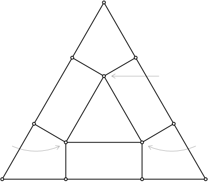
Figure 1. A spanning triangle for the vertices $a,b,c\in[X]_{0}$. A blue entry indicates a point which is known to lie in the monotone line in that factor. A blue circle represents the unique point in the monotone line for which the triple has height $0$. The labels in the regions indicate that each path in the boundary of that region lies within the indicated subspace.

There are four types of paths in this figure: six paths joining corner vertices to side vertices, three paths between adjacent side vertices, six paths from side vertices to interior vertices, and three interior paths. Consider first the path between $(a_{1},a_{2},a_{3})$ and $(\,\circ\,,b_{2},a_{3})$ in the upper left part of the figure. We may write the second vertex as $(a^{\prime}_{1},b_{2},a_{3})$ where $a^{\prime}_{1}$ is the unique point on $L_{1}$ such that the triple has height $0$. There is an edge path in $X_{2}$ from $a_{2}$ to $b_{2}$ of length $d_{X_{2}}(a_{2},b_{2})$. Combine this with the constant path $a_{3}$ in $X_{3}$, and the path in $L_{1}$ from $a_{1}$ to $a^{\prime}_{1}$ which compensates for the height changes in $X_{2}$, keeping the path in $[X]_{0}$. Put another way, this path in $[X]_{0}$ is the image of the path in $X_{2}\times X_{3}$ under the identification with $[L_{1}\times X_{2}\times X_{3}]_{0}$ given by the Embedding Lemma.

Next consider the path from $(a^{\prime}_{1},b_{2},a_{3})$ to the interior vertex $(\,\circ\,,b_{2},c_{3})=(a^{\prime\prime}_{1},b_{2},c_{3})$. This is defined by combining the constant path $b_{2}$ in $L_{2}$ with an edge path in $X_{3}$ from $a_{3}$ to $c_{3}$ of length $d_{X_{3}}(a_{3},c_{3})$, and interpreting as a path in $[L_{1}\times L_{2}\times X_{3}]_{0}$ via the isomorphism with $L_{2}\times X_{3}$.

To define the path in $[L_{1}\times L_{2}\times X_{3}]_{0}$ from $(a^{\prime}_{1},b_{2},a_{3})$ to $(a_{1},\,\circ\,,b_{3})=(a_{1},b^{\prime}_{2},b_{3})$ we proceed in a somewhat non-canonical manner. First use a path in $X_{3}$ from $a_{3}$ to $b_{3}$, of length $d_{X_{3}}(a_{3},b_{3})$, combined with the constant path $b_{2}$ in $L_{2}$, and a compensating motion in $L_{1}$, ending at a point $(a^{\prime\prime\prime}_{1},b_{2},b_{3})$. Then $(a_{1},b^{\prime}_{2})$ and $(a^{\prime\prime\prime}_{1},b_{2})$ have the same height in $L_{1}\times L_{2}$, so we can move horizontally from one to the other, in $d_{L_{2}}(b^{\prime}_{2},b_{2})$ steps. This path combines with the constant path $b_{3}$ in $X_{3}$ to give a path in $[X]_{0}$. Note that $d_{L_{2}}(b^{\prime}_{2},b_{2})\leqslant d_{X_{1}}(a_{1},b_{1})$ since the path from $(a_{1},b^{\prime}_{2},b_{3})$ to $(b_{1},b_{2},b_{3})$ (of length $d_{X_{1}}(a_{1},b_{1})$) projects to a path in $X_{2}$ from $b^{\prime}_{2}$ to $b_{2}$.

Lastly consider a path in $[L_{1}\times L_{2}\times L_{3}]_{0}$ between the interior vertices $(a^{\prime\prime}_{1},b_{2},c_{3})$ and $(a_{1},\,\circ\,,c_{3})=(a_{1},b^{\prime\prime}_{2},c_{3})$. Use a path in $L_{1}\times L_{2}$ from $(a^{\prime\prime}_{1},b_{2})$ to $(a_{1},b^{\prime\prime}_{2})$ of length at most $d_{X_{1}}(a_{1},a^{\prime\prime}_{1})+d_{X_{2}}(b_{2},b^{\prime\prime}_{2})$, and embed as a path in $[L_{1}\times L_{2}\times L_{3}]_{0}$. We have seen already that $d_{X_{1}}(a_{1},a^{\prime\prime}_{1})\leqslant d_{X_{2}}(a_{2},b_{2})+d_{X_{3}}(a_{3},c_{3})$ and $d_{X_{2}}(b_{2},b^{\prime\prime}_{2})\leqslant d_{X_{1}}(a_{1},b_{1})+d_{X_{3}}(b_{3},c_{3})$.

The rest of the paths are defined analogously according to their types. The length information just discussed is collected in Figure 2. We use the shorthand $\lvert{a_{i}-b_{i}}\rvert=d_{X_{i}}(a_{i},b_{i})$.

3pt $\lvert{a_{2}-b_{2}}\rvert$ [r] at 87 207 $\lvert{a_{3}-c_{3}}\rvert$ [l] at 168 207 $\lvert{a_{1}-b_{1}}\rvert$ [r] at 6 68 $\lvert{a_{1}-c_{1}}\rvert$ [l] at 249 68 $\lvert{b_{3}-c_{3}}\rvert$ [r] at 10 5 $\lvert{b_{2}-c_{2}}\rvert$ [l] at 245 5

$\lvert{a_{1}-b_{1}}\rvert+\lvert{b_{3}-c_{3}}\rvert$ [br] at 65 160 $+\,\lvert{a_{2}-b_{2}}\rvert+\lvert{a_{3}-c_{3}}\rvert$ [br] at 65 144

${\lvert{a_{3}-b_{3}}\rvert+\lvert{a_{1}-b_{1}}\rvert}$ [r] at 54 118

$\lvert{a_{3}-c_{3}}\rvert+\lvert{a_{2}-b_{2}}\rvert\,+$ [bl] at 191 160 $\lvert{a_{1}-c_{1}}\rvert+\lvert{b_{2}-c_{2}}\rvert$ [bl] at 191 144

${\lvert{a_{2}-c_{2}}\rvert+\lvert{a_{3}-c_{3}}\rvert}$ [l] at 200 118

${\lvert{b_{2}-c_{2}}\rvert+\lvert{a_{1}-c_{1}}\rvert}$ [b] at 129 48 ${+\,\lvert{b_{3}-c_{3}}\rvert+\lvert{a_{1}-b_{1}}\rvert}$ [t] at 126 51

${\lvert{b_{1}-c_{1}}\rvert+\lvert{b_{2}-c_{2}}\rvert}$ [t] at 128 15

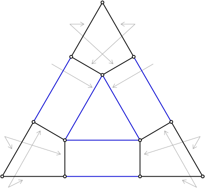
Figure 2. Lengths in the spanning triangle. For the blue paths, the lengths given are upper bounds only.

Definition 4.5.

The quantity $d_{0}(a,b)+d_{0}(b,c)+d_{0}(c,a)$ will be called the taut perimeter of the spanning triangle (not to be confused with the actual perimeter).

Remark 4.6.

From Figure 2 and (4.4) we can conclude:

1. The side from $a$ to $b$ has length at most $4d_{0}(a,b)$. Similarly, the other two sides have lengths at most $4d_{0}(b,c)$ and $4d_{0}(c,a)$.

2. Each of the seven regions has perimeter at most $4P$, where $P$ is the taut perimeter of the spanning triangle.

Remark 4.7.

Each of the subcomplexes labelling a region in Figure 1 is combinatorially isomorphic to one of the (sliced) cell complexes $X_{i}\times X_{j}$, $L_{i}\times X_{j}$, or $L_{i}\times L_{j}$, by the Embedding Lemma. All of these have Dehn functions that are $\preccurlyeq n^{\alpha}$ (here we use the assumption that $\alpha\geqslant 2$). Let $C$ be chosen so that $f(n)=Cn^{\alpha}$ is an upper bound for these Dehn functions. Then, by Remark 4.6(2), the triangle has filling area at most $7C(4P)^{\alpha}$ in $[X]_{0}$, where $P$ is the taut perimeter.

Remark 4.8.

The definition of the path along any side of the triangle depends only on its endpoints, and a choice of direction along the side (for the non-canonical path in the middle segment). Given two triples of vertices $a,b,c$ and $a,b,c^{\prime}$, spanning triangles for both can be made to agree along their sides from $a$ to $b$, by choosing the same direction on those sides.

A path along a side of a spanning triangle will be called a spanning path.

Short spanning paths

Consider the spanning path from $a$ to $b$ in Figure 1, and suppose that $a$ and $b$ have distance at most $1$ in $[X]_{0}$. If $a=b$ then the spanning path is a constant path, of length $0$. If $a\not=b$, the geodesic from $a$ to $b$ is a single edge in $[X]_{0}$, and we need to examine how this path may differ from the spanning path.

Lemma 4.9.

If $a$ and $b$ have distance $1$ in $[X]_{0}$ then the spanning path from $a$ to $b$ and the geodesic edge from $a$ to $b$ together form a loop with filling area at most $4$ in $[X]_{0}$.

Proof.

Since their distance is $1$, the points $a$ and $b$ differ in either one or two coordinates. If they differ in only one coordinate, then one finds that two of the three segments making up the spanning path are constant paths. (There are three cases, according to the coordinate where $a_{i}\not=b_{i}$.) The remaining segment has length $1$, as shown by Figure 2. Thus, up to reparametrization, the spanning path agrees with the geodesic path and the filling area is $0$.

Now suppose that $a$ and $b$ differ in two coordinates. Recall that the spanning path joins the following points, in order: $(a_{1},a_{2},a_{3})$, $(a_{1}^{\prime},b_{2},a_{3})$, $(a_{1}^{\prime\prime\prime},b_{2},b_{3})$, $(a_{1},b_{2}^{\prime},b_{3})$, and $(b_{1},b_{2},b_{3})$. There are now three cases. If $a_{1}=b_{1}$, then one also finds that $a_{1}^{\prime\prime\prime}=a_{1}=b_{1}$ and $b_{2}^{\prime}=b_{2}$. The image of the spanning path consists of two edges in the boundary of the cube $[a_{1}^{\prime},a_{1}]\times[a_{2},b_{2}]\times[b_{3},a_{3}]\subset X$, from $(a_{1},a_{2},a_{3})$ to $(a_{1}^{\prime},b_{2},a_{3})$ to $(a_{1},b_{2},b_{3})$. Together with the geodesic edge, these edges are the boundary of a horizontal $2$–cell in $[X]_{0}$, and the filling area is $1$.

If $a_{2}=b_{2}$ then one also has $a_{1}^{\prime}=a_{1}$. Let $[a_{1}^{\prime\prime\prime},b_{1}]$ denote the length two path in $X_{1}$ from $a_{1}^{\prime\prime\prime}$ to $b_{1}$, with midpoint $a_{1}$. Then $[a_{1}^{\prime\prime\prime},b_{1}]\times[b_{2}^{\prime},a_{2}]\times[a_{3},b_{3}]$ is a union of two cubes in $X$. The image of the spanning path consists of three edges on the boundary of these cubes. Together with the geodesic edge, they form a quadrilateral that bounds two triangles in $[X]_{0}$.

If $a_{3}=b_{3}$ then one also has $a_{1}^{\prime}=a_{1}^{\prime\prime\prime}$. Let $[a_{1}^{\prime},b_{1}]\subset X_{1}$ and $[a_{2},b_{2}^{\prime}]\subset X_{2}$ denote the paths of length $2$, with midpoints $a_{1}$ and $b_{2}$ respectively. The image of the spanning path consists of three edges in $[a_{1}^{\prime},b_{1}]\times[a_{2},b_{2}^{\prime}]\times\{a_{3}\}$, and the geodesic edge also lies in this subset. Choose a vertex $a_{3}^{\prime}\in X_{3}$ such that $d_{X_{3}}(a_{3},a_{3}^{\prime})=1$ and $(a_{1},b_{2},a_{3}^{\prime})\in[X]_{0}$. Such a vertex exists because $X_{3}$ is admissible. Then $[a_{1}^{\prime},b_{1}]\times[a_{2},b_{2}^{\prime}]\times[a_{3},a_{3}^{\prime}]\subset X$ is a union of four cubes in which the spanning path and geodesic path bound a disk made of four horizontal triangles, with common vertex $(a_{1},b_{2},a_{3}^{\prime})$. ∎

Proof of Theorem 4.2.

Simple connectedness of $[X]_{0}$ will follow from the remainder of the proof, in which we construct disks in $[X]_{0}$ filling any given loop.

Let $p$ be a closed edge path in $[X]_{0}$ of length $n>3$. There is a number $k\in{\mathbb{N}}$ such that $3\cdot 2^{k-1}<n\leqslant 3\cdot 2^{k}$. Let $\hat{p}$ be a path of length $\hat{n}=3\cdot 2^{k}$ obtained by padding $p$ with steps that move distance $0$. Note that $p$ and $\hat{p}$ have the same filling area.

Now consider the triangulated disk $D$ shown in Figure 3. It has $\hat{n}$ vertices along its boundary, $\hat{n}$ bigons around the outside, and $3\cdot 2^{k}-2$ triangles. Each triangle has a depth, where the central triangle has depth $0$, its neighbors have depth $1$, and so on. For $i=1,\dotsc,k$ there are $3\cdot 2^{i-1}$ triangles of depth $i$, and $k$ is the maximum depth that occurs.

3pt $1$ [b] at 72.5 154 $2$ [tr] at 10 47 $3$ [tl] at 136 47

$1$ [t] at 73 8 $2$ [bl] at 136 114 $3$ [br] at 10 114

$3$ [bl] at 108 143 $1$ [l] at 144.5 81 $2$ [tl] at 108 18 $3$ [tr] at 38.5 18 $1$ [r] at 1 81 $2$ [br] at 38.5 143.5

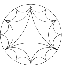
Figure 3. Filling the loop with spanning triangles. A $3$–coloring of the vertices is shown.

There is a $3$–coloring of the vertices of $D$: each vertex $v$ can be assigned a coordinate $\kappa(v)\in\{1,2,3\}$ such that $\kappa(v)\not=\kappa(u)$ whenever $u,v$ bound an edge in $D$. Now identify the boundary of $D$ with the path $\hat{p}$. Each vertex of $D$ is identified with a vertex in $[X]_{0}$ and has coordinates in $X$. Writing $v=(v_{1},v_{2},v_{3})$, choose a monotone line $L_{v}$ in $X_{\kappa(v)}$ which contains the point $v_{\kappa(v)}$.

Each triangle in $D$ can now be filled with a spanning triangle for its vertices, using the three vertices and the three monotone lines chosen for those vertices. The $3$–coloring ensures that this data conforms to the requirements of the starting data for spanning triangles. We start by filling the central triangle, and then proceed to fill triangles in order of depth. Each new triangle to be filled meets the previously filled triangles in a single edge, so by Remark 4.8, the spanning triangle can be chosen to use the same spanning path for that edge. Then the spanning triangles fit together to yield a filling of $D$, minus the bigons.

Declare the depth of an interior edge in $D$ to be the minimum of the depths of its neighboring triangles. Note that an edge of depth $i$ joins points on the boundary that bound a boundary arc of length $2^{k-i}$, and so these points have distance at most $2^{k-i}$ in $[X]_{0}$.

The central triangle has taut perimeter at most $\hat{n}$, and the taut perimeter of a depth $i$ spanning triangle ($i=1,\dotsc,k$) is at most $2^{k-(i-1)}+2^{k-i}+2^{k-i}=2^{k-i+2}$. By Remark 4.7 the central spanning triangle has area at most $7C(4\hat{n})^{\alpha}=7\cdot 12^{\alpha}C\cdot 2^{k\alpha}$ and a depth $i$ spanning triangle has area at most $7\cdot 4^{\alpha}C(2^{k-i+2})^{\alpha}$. Now the total area of the spanning triangles is at most

$$7\cdot 12^{\alpha}C\cdot 2^{k\alpha}+\sum_{i=1}^{k}3\cdot 2^{i-1}\cdot 7\cdot 4^{\alpha}C(2^{k-i+2})^{\alpha}\ =\ 7\cdot 12^{\alpha}C\cdot 2^{k\alpha}+21C\cdot 2^{k\alpha+4\alpha-1}\sum_{i=1}^{k}2^{(1-\alpha)i}$$

$$<\ 7\cdot 12^{\alpha}C\cdot 2^{k\alpha}+21C\cdot 2^{k\alpha+4\alpha-1}$$

$$<\ 28C\cdot 12^{4\alpha}\cdot 2^{k\alpha}.$$

Each bigon has filling area at most $4$, by Lemma 4.9. Then the filling area of $p$ is at most

$$28C\cdot 12^{4\alpha}\cdot 2^{k\alpha}+4\cdot 3\cdot 2^{k}\ <\ (28C+1)\cdot 12^{4\alpha}\cdot 2^{k\alpha}$$

$$=\ (28C+1)\cdot 12^{4\alpha}\cdot 2^{\alpha}\cdot 3^{-\alpha}\cdot(3\cdot 2^{k-1})^{\alpha}$$

$$<\ ((28C+1)\cdot 12^{4\alpha}\cdot 2^{\alpha}\cdot 3^{-\alpha})n^{\alpha}$$

since $3\cdot 2^{k-1}<n$. Therefore $\delta_{[X]_{0}}(n)\leqslant Kn^{\alpha}$ where $K=(28C+1)\cdot 12^{4\alpha}\cdot 2^{\alpha}\cdot 3^{-\alpha}$. ∎

References

- [1] A. Abrams, N. Brady, P. Dani, M. Duchin, and R. Young, Pushing fillings in right-angled Artin groups, J. Lond. Math. Soc. (2), 87 (2013), pp. 663–688.
- [2] M. Amchislavska and T. Riley, Lamplighters, metabelian groups, and horocyclic products of trees. To appear in L’Enseignement Mathématique, http://arxiv.org/abs/1405.1660.
- [3] G. Baumslag, M. R. Bridson, C. F. Miller, III, and H. Short, Finitely presented subgroups of automatic groups and their isoperimetric functions, J. London Math. Soc. (2), 56 (1997), pp. 292–304.
- [4] M. Bestvina and N. Brady, Morse theory and finiteness properties of groups, Invent. Math., 129 (1997), pp. 445–470.
- [5] R. Bieri, Homological dimension of discrete groups, Mathematics Department, Queen Mary College, London, 1976. Queen Mary College Mathematics Notes.
- [6] N. Brady, M. R. Bridson, M. Forester, and K. Shankar, Snowflake groups, Perron-Frobenius eigenvalues and isoperimetric spectra, Geom. Topol., 13 (2009), pp. 141–187.
- [7] M. R. Bridson. personal communication.
- [8] , Doubles, finiteness properties of groups, and quadratic isoperimetric inequalities, J. Algebra, 214 (1999), pp. 652–667.
- [9] , The geometry of the word problem, in Invitations to geometry and topology, vol. 7 of Oxf. Grad. Texts Math., Oxford Univ. Press, Oxford, 2002, pp. 29–91.
- [10] M. R. Bridson and A. Haefliger, Metric spaces of non-positive curvature, vol. 319 of Grundlehren der Mathematischen Wissenschaften [Fundamental Principles of Mathematical Sciences], Springer-Verlag, Berlin, 1999.
- [11] M. W. Davis, The geometry and topology of Coxeter groups, vol. 32 of London Mathematical Society Monographs Series, Princeton University Press, Princeton, NJ, 2008.
- [12] W. Dison, An isoperimetric function for Bestvina-Brady groups, Bull. Lond. Math. Soc., 40 (2008), pp. 384–394.
- [13] W. Dison, M. Elder, T. R. Riley, and R. Young, The Dehn function of Stallings’ group, Geom. Funct. Anal., 19 (2009), pp. 406–422.
- [14] C. Druţu, Filling in solvable groups and in lattices in semisimple groups, Topology, 43 (2004), pp. 983–1033.
- [15] S. M. Gersten, Finiteness properties of asynchronously automatic groups, in Geometric group theory (Columbus, OH, 1992), vol. 3 of Ohio State Univ. Math. Res. Inst. Publ., de Gruyter, Berlin, 1995, pp. 121–133.
- [16] M. Gromov, Asymptotic invariants of infinite groups, in Geometric group theory, Vol. 2 (Sussex, 1991), vol. 182 of London Math. Soc. Lecture Note Ser., Cambridge Univ. Press, Cambridge, 1993, pp. 1–295.
- [17] D. Groves. personal communication.
- [18] J. Stallings, A finitely presented group whose 3-dimensional integral homology is not finitely generated, Amer. J. Math., 85 (1963), pp. 541–543.
- [19] R. Young, The Dehn function of , Ann. of Math. (2), 177 (2013), pp. 969–1027.