Model atmospheres of irradiated exoplanets:
The influence of stellar parameters, metallicity, and the C/O ratio
Abstract
Many parameters constraining the spectral appearance of exoplanets are still poorly understood. We therefore study the properties of irradiated exoplanet atmospheres over a wide parameter range including metallicity, C/O ratio and host spectral type. We calculate a grid of 1-d radiative-convective atmospheres and emission spectra. We perform the calculations with our new Pressure-Temperature Iterator and Spectral Emission Calculator for Planetary Atmospheres (PETIT) code, assuming chemical equilibrium. The atmospheric structures and spectra are made available online. We find that atmospheres of planets with C/O ratios 1 and 1500 K can exhibit inversions due to heating by the alkalis because the main coolants CH4, H2O and HCN are depleted. Therefore, temperature inversions possibly occur without the presence of additional absorbers like TiO and VO. At low temperatures we find that the pressure level of the photosphere strongly influences whether the atmospheric opacity is dominated by either water (for low C/O) or methane (for high C/O), or both (regardless of the C/O). For hot, carbon-rich objects this pressure level governs whether the atmosphere is dominated by methane or HCN. Further we find that host stars of late spectral type lead to planetary atmospheres which have shallower, more isothermal temperature profiles. In agreement with prior work we find that for planets with 1750 K the transition between water or methane dominated spectra occurs at C/O 0.7, instead of 1, because condensation preferentially removes oxygen.
Subject headings:
methods: numerical — planets and satellites: atmospheres — radiative transferI. Introduction
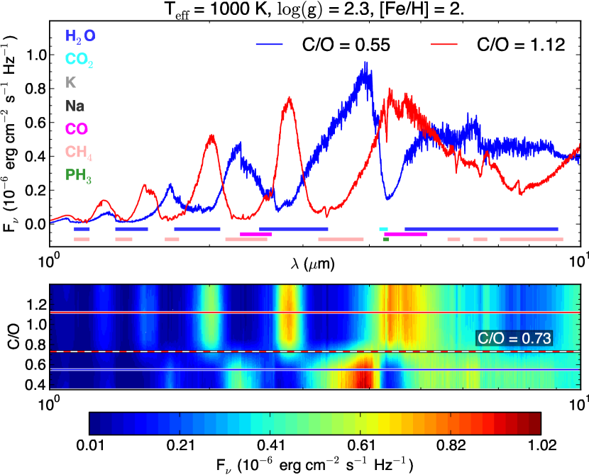
In a number of existing studies the range of possible C/O ratios in protoplanetary disks and the resulting implications for the C/O ratios in the gaseous envelopes of extrasolar planets is investigated (see, e.g., Öberg et al. 2011; Ali-Dib et al. 2014; Helling et al. 2014; Marboeuf et al. 2014; Thiabaud et al. 2014). These kind of studies are interesting, as they may help to predict the spectral appearance of atmospheres of planets formed via different pathways in the circumstellar disks. In a further example, Madhusudhan et al. (2014a) studies the range of possible C/O ratios for 2 different disk models, depending on the formation and migration mechanism invoked to form hot jupiters. The result of these studies is that large planetary C/O ratios, close to unity, are possible even when considering disks of solar composition (the solar value is C/O⊙ 0.55, see Asplund et al. 2009). For disks with supersolar C/O ratios the planetary C/O ratios should be even higher, although stars with C/O ratios close to and bigger than 1 may be quite rare (Fortney 2012). The C/O ratio is particularly interesting for the spectral appearance of exoplanets because for high enough temperatures ( 1000 K) a C/O giant planet will have appreciable amounts of H2O in its atmosphere and almost no CH4, whereas for C/O the situation is the opposite and CH4 is much more abundant than H2O. This transition happens quite sharply (see, e.g., Kopparapu et al. 2012; Madhusudhan 2012). Furthermore, condensation processes can potentially lead to local C/O ratios of 1-2 in the gas phase, even if the global atmospheric C/O ratio is smaller than 1 (see Helling et al. 2014). The reason this is for the locking up of oxygen in silicates, as has already been suggested by Fortney et al. (2006).
Both H2O and CH4 have strong absorption features and their main absorption bands between 1.3 and 5 m are alternately located in wavelength space. Thus hot gaseous planets with C/O 1 and C/O 1 in the spectrally active regions should be quite easily distinguishable and might give hints on the planet’s formation history such as the location of formation in the protoplanetary disk and its migration through it (Madhusudhan et al. 2014a). For even higher temperatures ( 1750 K), and C/O 1, HCN takes over as the most important carbon-carrying infrared absorber as it becomes more abundant than CH4 in the spectrally active parts of the atmospheres (see, e.g., Moses et al. 2013). “Spectrally active” denotes the regions where the radiation seen in the planet’s emergent spectrum originates. The respective atmospheres are then not dominated by CH4 anymore, but by HCN. Distinguishing H2O and HCN absorption features should be possible, due to the different spectral signatures of HCN and H2O in the NIR and IR. Therefore a distinction between O and C dominated atmospheres is possible also at high temperatures.
Motivated by the fundamentally different spectral appearances of the two C/O cases, Madhusudhan (2012) proposed a 2-d classification scheme for characterizing giant extrasolar planets, using the C/O ratio and the incident stellar flux as dimensions. In his work, the importance of CH4 for the C/O 1 cases is most strongly emphasized, but the possible importance of HCN and C2H2 is mentioned as well. A 1-d classification scheme for hot giant planets, based only on the stellar flux, had already been proposed by Fortney et al. (2008) before, featuring “cold” hot jupiters without a temperature inversion and “hot” hot jupiters with a temperature inversion caused by TiO and VO absorption.
| Opacity source | Spectral range [m] | Line list | Partition function | Pressure broadening |
|---|---|---|---|---|
| CH4 | 0.83 | Yurchenko and Tennyson (2014) | (a) | (a) |
| CH4 | 0.86 | Rothman et al. (2013) | Fischer et al. (2003) | , Rothman et al. (2013) |
| C2H2 | 1 16.5 | Rothman et al. (2013) | Fischer et al. (2003) | , Rothman et al. (2013) |
| CO | 1.18 | Rothman et al. (2010) | Fischer et al. (2003) | , Rothman et al. (2010) |
| CO | 0.112 0.43 | Kurucz (1993) | Fischer et al. (2003) | Eq. (15), Sharp and Burrows (2007) |
| CO2 | 1 38.76 | Rothman et al. (2010) | Fischer et al. (2003) | , Rothman et al. (2010) |
| H2S | 0.88 | Rothman et al. (2013) | Fischer et al. (2003) | , Rothman et al. (2013) |
| H2 | 0.28 | Rothman et al. (2013) | Fischer et al. (2003) | , Rothman et al. (2013) |
| H2 | 0.08 0.18 | Kurucz (1993) | Fischer et al. (2003) | Eq. (15), Sharp and Burrows (2007) |
| HCN | 2.92 | Harris et al. (2006), | Fischer et al. (2003) | Eq. (15), Sharp and Burrows (2007) |
| Barber et al. (2014) | ||||
| H2O | 0.33 | Rothman et al. (2010) | Fischer et al. (2003) | , Rothman et al. (2010) |
| K | 0.05 | Piskunov et al. (1995) | Sauval and Tatum (1984) | N. Allard, Schweitzer et al. (1996) |
| Na | 0.1 | Piskunov et al. (1995) | Sauval and Tatum (1984) | N. Allard, Schweitzer et al. (1996) |
| NH3 | 1.43 | Rothman et al. (2013) | Fischer et al. (2003) | , Rothman et al. (2013) |
| OH | 0.52 | Rothman et al. (2010) | Fischer et al. (2003) | , Rothman et al. (2010) |
| PH3 | 2.78 | Rothman et al. (2013) | Fischer et al. (2003) | , Rothman et al. (2013) |
However, some “hot” hot jupiters are not thought to have a inversion, contradicting the 1-d classification system. Madhusudhan (2012) argued that this could possibly be explained using the 2-d classification scheme, as TiO and VO should not be very abundant in planets with a high C/O ratio. In addition, there could be further reasons why TiO and VO should not be in the upper part of the atmosphere, e.g. due to settling and inefficient vertical mixing, cold-trap depletion or photodissociation (Spiegel et al. 2009; Showman et al. 2009; Parmentier et al. 2013; Knutson et al. 2010).
Observational evidence for planets with C/O 1 is scarce and the most prominent case, WASP-12b (Madhusudhan et al. 2011), is controversial (Crossfield et al. 2012; Swain et al. 2013; Stevenson et al. 2014). Current analyses of the photometric data indicate a C/O ratio 1: Line et al. (2014) estimated C/O ratios for 9 hot jupiters and found that while in 7 out of 9 cases (HD 209458b, GJ436b, HD 149026b, WASP-12b, WASP-19b, WASP-43b, TrES-2b) a C/O value of 1 was within their 1 confidence interval, in 6 out of 9 cases the solar value was within the 1 interval as well. Benneke (2015) analyzed 8 hot jupiters (HD 209458b, WASP-19b, WASP-12b, HAT-P-1b, XO-1b, HD189733b, WASP-17b and WASP-43b) using a self-consistent retrieval analysis, ruling out C/O 1 for all of them. Clearly the quality and quantity of the photometric and spectroscopic observations needs to improve before more conclusive results can be obtained for many of these planets (Line et al. 2013).
A further example for a planet with a C/O ratio close to 1 is HR 8799b, for which C/O = or has been estimated (Lee et al. 2013), depending on whether clouds are included in the model or not.
Although all the C/O ratios obtained by the above studies are depending on the assumptions made in the various retrieval models, the current analysis of data does not indicate any planet with C/O 1. Further, while the current quality of data is still too low for obtaining reliable retrieval results in many cases, upcoming observing facilities such as JWST should greatly help to decipher the composition of hot jupiters.
In conclusion, the C/O ratio, together with the effective temperature, should be a key parameter constraining a hot jupiter’s spectral appearance and thus we want to study how the interplay between the C/O ratio and other parameters affect the atmospheres. Systematic studies of exoplanet atmospheres have been published in the literature before (see, e.g., Sudarsky et al. 2003), and although the C/O has been suggested to be of importance already a decade ago (Seager et al. 2005), no systematic study of the atmospheric characteristics as a function of the C/O ratio has been carried out so far. Therefore, we publish a grid of emission spectra and pressure temperature () structures for self-consistent hot jupiters atmospheres for varying C/O ratio, [Fe/H], distance to the star, stellar host spectral type and planetary .
The results were calculated with our new Pressure-Temperature Iterator and Spectral Emission Calculator for Planetary Atmospheres (PETIT) code. PETIT solves the 1-d plane parallel structure of the atmosphere assuming local thermal equilibrium (LTE), radiative equilibrium or convection and equilibrium chemistry. Our goal is to investigate the behavior of planetary atmospheres in the parameter space covered by our grid. Furthermore we make the atmospheric -structures, abundance profiles, and resulting spectra publicly available for use in, e.g., the evaluation of observational data of planetary emission spectra.
In Section II we introduce our code and explain its individual modules. We also show some of the tests we carried out to check the results of our code for consistency. In Section III we discuss how the assumptions in our code constrain the parameter range of the atmospheric grid. In Section IV we report on how the grid was set up and how the calculations were carried out. The results can be found in Section V, the discussion and conclusions are in Section VI.
II. Description of the code
II.1. Opacity database
The current version of our opacity database comprises atomic and molecular line and continuum opacities from ultra-violet to infrared wavelengths. So far only absorption processes are treated. Scattering of incoming stellar radiation by molecules in the planetary atmosphere causes the stellar photons to traverse, on average, a somewhat longer distance through the atmosphere before reaching a certain pressure level. Hence, the photons will on average be absorbed at slightly lower pressures (higher altitudes) than if absorption only is considered. Because the reported optical albedos of hot jupiters are very low, in the low single digit percentage range, as summarized by Madhusudhan et al. (2014b), absorption appears much more important than scattering in these objects. Therefore, include only absorption in the radiative transfer calculation One exception is mentioned, however, with Kepler 7-b having a geometric albedo of 0.32 0.03 (Demory et al. 2011).
II.1.1 Molecular and atomic line opacities
A list of all line opacity sources, together with a reference to the corresponding line lists, pressure broadening parameters and partition functions can be found in Table 1. Our method to speed up molecular opacity calculations is explained in Appendix A.
All molecular and atomic lines are considered to have a Voigt profile (except for the Na and K doublet) and no truncation of the lines at large distances from the line cores has been applied. This choice of the far-wing treatment of the line shape is arbitrary. It is well known that the molecular lines should become sub-Lorentzian at large distances from the line core (see e.g., Freedman et al. 2008, and the references therein). However, the position of the cut-off, and the line wing shape itself, depend on the pressure and temperature and the perturber gases which broaden the molecular and atomic transitions. The choice to use Voigt profiles and not truncating the lines is thus only made because of the lack of knowledge regarding the actual line profiles. Grimm and Heng (2015) show that the differences when applying no line cut-off, when compared to an arbitrary cut-off, are at least of the order of 10 % when considering layer transmissions. In order to calculate the Voigt profiles we use the code provided by Humlícek (1982).
The calculations are performed on a pressure-temperature grid with 10 grid points in pressure going from 10-6 to 103 bars (equidistantly spaced in log-space). Because the line wing strength due to pressure broadening is well behaved (the strength is simply linear in ), we found this grid spacing to be sufficient when interpolating to the actual pressures of interest. The temperature grid consists of 10 points going from 200 to 3000 K, equidistantly spaced in log-space as well. Opacities with temperatures 270 K are only calculated up to 1 bar, temperatures up to 670 K only up to 10 bar, and temperatures up to 900 K only up to 100 bar. This choice was made because it was found, using the simple Guillot (2010) atmospheric model, that even cold planets such as Jupiter and Uranus should not be cooler than 270, 670 and 900 K at the pressures cited above. As we concentrate on hot jupiters in this paper we therefore did not extend the grid to cool temperatures at high pressures. We plan to extend the grid in the future, however. In total the above considerations yield 87 pressure–temperature grid-points.
Our fiducial wavelength range goes from 110 nm to 250m. We calculate the opacities in this range on a grid with a spacing of . This resolution is sufficient to resolve the line cores at all pressures and temperatures. From these calculations we construct opacity distribution tables (k-tables) for later use (see Section II.3.1). These tables are then interpolated to the pressure-temperature values of interest.
Most of the line lists are obtained from the HITRAN/HITEMP databases (Rothman et al. 2013, 2010), together with additional data from the VALD, Kurucz and ExoMol line lists (Piskunov et al. 1995; Kurucz 1993; Harris et al. 2006; Barber et al. 2014). For methane we use HITRAN for temperatures below 300 K. For temperatures above 300 K the ExoMol cross-sections are used (Yurchenko and Tennyson 2014), as this line list is much more complete at higher temperatures. The ExoMol cross-sections (in units of cm2 molecule-1) can be obtained, tabulated as a function of wavelength, from the ExoMol website. No pressure broadening has been applied when calculating these cross-sections, as pressure broadening information is not readily available. However, due to the sheer number of methane lines the cross-sections should be dominated by the Gaussian line cores. In general, for all molecular and atomic line opacities, pressure broadening information is often not available, especially when taking into account arbitrary mixtures of various molecular and atomic gaseous species. We therefore estimate the pressure broadening by using the air broadening coefficients of the HITRAN/HITEMP database when these are available for a given molecule of interest. In cases where this information is missing as well we resort to the use of the pressure broadening approximation provided by Eq. (15) in Sharp and Burrows (2007).
A special line shape treatment is needed when considering the Na (589.16 & 589.76 nm) and K (766.7 & 770.11 nm) doublet lines. Na and K are very important to correctly describe the atmospheric absorption in the optical, as these two species are one of the main absorbers in this spectral range and their line wings act as a pseudo-continuum contribution to the total opacity (see, e.g., Sharp and Burrows 2007; Freedman et al. 2008). Different groups have tried to estimate the line shapes for Na and K taking into account collisions with H2 and He (Burrows and Volobuyev 2003; Allard et al. 2003; Zhu et al. 2006), and the efforts are ongoing (Allard et al. 2012). In particular Allard et al. (2003) showed that for brown dwarfs the use of correct Na and K wing profiles improves the agreement between synthetic spectra and observations. The line profiles we use for Na were obtained from Nicole Allard (private communication) using Rossi and Pascale (1985) pseudo potentials. For K we use the profiles available on the website of Nicole Allard111http://mygepi.obspm.fr/~allard/alkalitables.html, which include C2v and C∞v interaction symmetries. As H2 should be the main perturber for alkali atoms in the atmosphere of giant planets, only H2-broadening is currently considered. The other lines of Na and K, which are much weaker than the doublet transitions, are modeled using van der Waals (vdW) broadening as described in Schweitzer et al. (1996):
| (1) |
where is the van der Waals interaction constant, is the mean relative velocity between H2 and the alkali atom, is the H2 number density and is a dimensionless number. Schweitzer et al. (1996) report that , but it is a factor of 10 smaller in Sharp and Burrows (2007). We found that if we want to reproduce the vdW line widths given in Allard et al. (2007), then we need to use the smaller value. The required ionization energies were taken from the NIST database222http://www.nist.gov/pml/data/asd.cfm.
Because the non-Lorentzian line profile calculations for the Na and K wings by Nicole Allard are only valid up to a certain H2 density (1020 or 1019 cm-3 for Na or K, respectively) we revert to the use of Voigt profiles for higher densities. This occurs in the range of 3-30 bars in hot jupiters, where the atmosphere becomes optically thick in the IR and the stellar light has been absorbed.
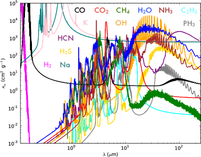
In Figure 1 we show all molecular and atomic line opacities of our database at a temperature of 1650 K and a pressure of 100 bar in our fiducial wavelength space going from 110 nm to 250 m. The pressure of 100 bars is far higher than where the radiation in the planetary emission spectra usually stems from. However, as the pressure broadening smoothes out individual lines, the large scale opacity features can more easily be seen at higher pressures. This figure has been generated from our opacity distribution database and shows the mean value of every wavelength subgrid which are spaced at a resolution of . Here, is the cumulative opacity distribution function, see Section II.3.1 for more information.
VO and TiO opacities have not been added yet. We explained in Section I that the role of these two absorbers is quite controversial, as they might not be present in the atmospheres due to a potential rain-out, cold-trap capture or photodissociation. Nonetheless, we plan to add VO and TiO opacities in the next version of the code.
II.1.2 Continuum opacities
As a continuum opacity source we currently consider collision induced absorption (CIA) arising from H2-H2 and H2-He collisions. Tabulated data and programs from Borysow et al. (1988, 1989); Borysow and Frommhold (1989); Borysow et al. (2001); Borysow (2002) were used to obtain the cross-sections333Tables and code were obtained from http://www.astro.ku.dk/~aborysow/programs/index.html.
II.2. Stellar spectra
For the host star spectral templates we use PHOENIX models of main-sequence stars which have evolved to 1/3 of their main sequence lifetime.444The results for the stellar spectra depend only very mildly on this choice, the main effect being that the stars slowly increase their luminosity with time. Because the transiting hot jupiters that can be best studied orbit K-type stars, which typically have ages less than half of their main sequence lifetime, we chose a value of 1/3. For the stellar evolution we use Yonsei-Yale tracks (Yi et al. 2001; Kim et al. 2002; Yi et al. 2003; Demarque et al. 2004) as well as the evolutionary calculations of Baraffe et al. (1998). More details can be found in van Boekel et al. (2012).
II.3. Code structure and modules
The basic principle for solving for the atmospheric structure is based on Dullemond et al. (2002), which we adapted to the case of 1-d plane parallel planetary atmospheres. The code starts with an initial guess for the temperature structure, computes the corresponding molecular and atomic abundances and the resulting opacities and then calculates the temperature assuming radiative-convective equilibrium. The code then starts again with the newly found - structure until the solution converges. Because the -structure, the abundances and opacities mutually depend on each other, we solve for atmospheric structure in an iterative fashion.
From a given atmospheric temperature structure we obtain the molecular abundances using the CEA equilibrium chemistry code (Gordon and McBride 1994; McBride and Gordon 1996). When the current opacities are calculated, we solve the full angle and frequency dependent radiative transfer problem of the planetary radiation field. From this we obtain the intensity-mean, flux-mean and Planck mean opacities as well as the variable Eddington factors. These opacities and Eddington factors are then used in the Variable Eddington Factor (VEF) module to find the temperature structure using the moments of the radiation field (see, e.g., Hubeny and Mihalas 2014). The temperature is found using a two-stream approximation for the planetary and stellar radiation field. Furthermore we check if a given atmospheric layer is convective by applying the Schwarzschild criterion. We switch to an adiabatic temperature gradient in the layers that are found to be convective.
The iteration is stopped once the maximum
change in temperature between the current iteration and the temperature found 60 iterations ago is smaller than
0.01 K and if the planetary emerging flux obtained from the full angle and frequency dependent radiative transfer solutions is equal to the imposed
total flux with a relative maximum deviation of 0.001.
In rare situations the iteration will slowly oscillate within a a given temperature range and not find a solution
and therefore not converge to a solution with a maximum flux deviation of 0.001.
In this case we flag the files of the atmospheric structures with _nconvergence_YYY where YYY is the relative
deviation to the imposed flux in percent.
In sections II.3.1, II.3.2 and II.3.3 we give further detailed information on the code modules (full radiative transfer module, VEF temperature iteration module and the equilibrium chemistry module, respectively).
II.3.1 Radiative transfer module
In protoplanetary disks, for which the VEF based approach by Dullemond et al. (2002) has been developed, the main contribution to the total opacity is coming from dust and ice grains (see, e.g., Semenov et al. 2003). An important feature of dust grain opacities is that they vary only slowly with wavelength, making it possible to use a small number of wavelength grid points.
In the case of planetary atmospheres molecules contribute strongly to the total opacity. The molecules which are important for the spectrum can have hundreds of millions to tens of billions of very sharply peaked lines (see, e.g., Rothman et al. 2010; Yurchenko and Tennyson 2014, for H2O and CH4, respectively). Therefore, especially at low pressures, radiative transfer calculations need to be carried out at high spectral resolution. We thus have adopted the opacity distribution method and the correlated-k (c-k) assumption (Goody et al. 1989; Fu and Liou 1992; Lacis and Oinas 1991) to carry out our radiative transfer calculations. Opacity distribution tables (k-tables) should yield a good description of the detailed high resolution opacities while keeping the numerical costs of the radiative transfer calculations minimal.
We combine the k-tables of all molecular species contributing to the total opacity using a fast combination method which has a computational cost linear in the number of species , see Section B.
The calculations to obtain the mean opacities and Eddington factors are carried out on our fiducial grid (going from 110 nm to 250 m) with a grid spacing of , which results in 78 spectral bins. In order to test the accuracy of these results we have carried out calculations at a grid spacing of as well, but the differences in the results are negligible.
To calculate the emission spectrum of an atmosphere after the -structure has converged we carry out a c-k radiative transfer calculation at a grid spacing of , which results in 7729 spectral bins.
In every spectral bin of the = 10, 50 and 1000 cases we employ a -grid. replaces the spectral coordinate or in c-k, it is equal to the value of the cumulative opacity distribution function, i.e.
| (2) |
where is the fraction of the opacity values between and within a given frequency interval. We carry out the radiative transfer calculation using , instead of the frequency or wavelength. The frequency averaged mean of any radiative quantity within the spectral bin can then be calculated as
| (3) |
where is the quantity corresponding to in -space within the spectral bin of interest.
For the case we approximate on a grid of 20 Gaussian quadrature points, consisting of a 10 point Gaussian quadrature grid going from to and a 10 point Gaussian quadrature grid going from to .
For the = 10 and 50 cases we take a finer grid in . The g-grid has 36 points, consisting of a 6 point Gaussian quadrature grid ranging from to , an 8 point Gaussian grid ranging from to , a 20 point Gaussian grid ranging from to and a two point trapezoidal quadrature grid ranging from to 1.
The different methods for obtaining the combined c-k opacity of all species at the resolutions of , = 10 and = 50 are explained in Section B.
The radiative transfer calculations are made using a 2nd order Feautrier method, considering 20 (i.e. cos ) angles on a 20-point Gaussian quadrature grid.
II.3.2 Variable Eddington factor method
A description of the variable Eddington factor method, and how we use it to find the temperature in the atmosphere, can be found in Section C.
In our code the radiation from the star can be received in 3 different ways: (i) The angle between the atmospheric vertical and the stellar irradiation is ; (ii) The stellar flux is absorbed by the planet with a cross-section of but distributed over the dayside hemisphere (dayside average): The incident vertical irradiation is reduced by a factor of ; (iii) The stellar flux is absorbed by the planet with a cross-section of but distributed over the full area (global average): The incident vertical irradiation is reduced by a factor of . In the dayside or global average cases the stellar irradiation field is treated to be shining at the atmosphere isotropically. For our atmospheric grid we chose option (ii). We therefore assume that there is no efficient redistribution of the insolation energy to the night side. We will revisit the validity of this assumption in Section III.
II.3.3 Equilibrium Chemistry
We use the NASA Chemical Equilibrium with Applications (CEA) code by Gordon and McBride (1994); McBride and Gordon (1996). The code minimizes the total Gibbs free energy of all possible species while conserving the number of atoms of every atomic species. Given a pressure and temperature together with the atomic composition of the gas the output of the code is the mass and number fraction of all possible outcome species (atoms, ions, molecules), the resulting density, as well as the adiabatic temperature gradient of the gas mixture.
II.4. Testing the code
To characterize the quality of the results produced by the PETIT code a series of tests were carried out.
II.4.1 Correlated-k radiative transfer
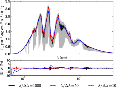
First it was tested whether the correlated-k opacity combination methods introduced in Section B yield results of sufficient accuracy. To this end we calculated the emission spectrum of a hot jupiter at our three different resolutions , using correlated-k and compared to the results of a line-by-line calculation at a resolution . As an example -structure we took a self-consistent result from our code for a 1 , 1 planet555Where and are Jupiter’s mass and radius, respectively. around a sun-like star with an effective temperature = 5730 K with radius . The planet was assumed to be in a circular orbit at a distance of = 0.04 AU, have an internal temperature = 200 K and a C/O ratio of 1.17. We calculated the -structure for a day-side averaged hemisphere.
The resulting emission spectra of the planet can be seen in the upper panel of Figure 2. In the lower panel we calculate the relative errors of the correlated-k calculations when compared to the frequency averaged line-by-line calculation. If the c-k assumption was perfectly valid the error would be zero, as the flux values of a c-k calculation at resolution (e.g.) 10 should be identical to the flux of a higher resolution line-by-line calculation, after having been frequency averaged to the same resolution. One sees that in regions of appreciable flux the relative deviation between the rebinned line-by-line calculation and the correlated-k calculations is always smaller than 5 and usually much less. Thus our results are within the accuracy limits commonly found for correlated-k (see, e.g., Fu and Liou 1992; Lacis and Oinas 1991).
II.4.2 Energy balance
As a next step we tested whether the converged solution is consistent with the input parameters. This was done by checking whether the final -structure, together with the molecular abundances and their corresponding opacities gives rise to the correct total emergent flux. For a day-side averaged -spectrum the total emergent flux should be
| (4) |
Furthermore, deep within the atmosphere, but at lower pressure than the radiative-convective boundary , the radiation field only needs to carry the internal flux of the planet. The reason for this is that all the stellar flux has been absorbed. One thus finds that
| (5) |
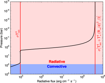
Even further down the -structure will eventually become convective such that the radiative flux becomes negligible when compared to the convective flux. In Figure 3 one can see the result obtained from integrating the angle and frequency dependent radiation field of the correlated-k structure calculation. The radiation field was integrated to yield the bolometric flux in the atmosphere as a function of pressure. It can be seen that the surface flux converges to . Furthermore, at approximately 3 bar, the stellar flux has been absorbed and the radiative flux is equal to . At even higher pressures ( bar) the atmosphere becomes convective and the flux transported by radiation starts to dwindle. The radiation field thus behaves as expected and the converged solution indeed fulfils the input parameters of the problem. The relative difference between the converged solution of the total emergent flux and the imposed flux was 0.08 %.
II.4.3 Comparison to data: HD 189733b
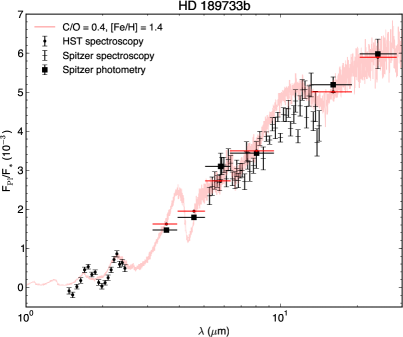
In order to get to get a qualitative impression of the comparability of our calculations with actual data we chose to look at HD 189733b, as it has quite a lot of available measurements. We used the following data: Spitzer IRAC photometry: 3.6 and 4.5 m (Knutson et al. 2012), 5.8 m (Charbonneau et al. 2008) and 8 m (Agol et al. 2010), Spitzer IRS broadband at 16 m , Spitzer MIPS at 24 m (both Charbonneau et al. 2008), HST NICMOS spectroscopy (Swain et al. 2010) and Spitzer IRS spectroscopy (Grillmair et al. 2008). For the stellar, planetary and orbital parameters we adopted = 5040 K, = 0.756 , = 1.138 (Torres et al. 2008), = 1.137 (Butler et al. 2006; Agol et al. 2010) and = 0.031 AU (Butler et al. 2006). The comparison between the data and our model for HD 189733b assuming C/O = 0.4 and [Fe/H] = 1.4 can be seen in Figure 4. We chose these values as they are within the Bayesan regions with the highest credibility identified by Benneke (2015) for this planet. One can see that between 5 and 8 m our model fits the IRS spectroscopy quite well, including the water feature at 6.6 m, while it is somewhat too high at larger wavelengths. While the IRAC points for wavelengths below 8 m are not fitted very well, the IRAC photometry point at 8 m, the IRS broadband and MIPS photometry points are all well fitted by our model. Further, the water absorption features between 1.5 and 2.5 m in our model seem to correlate with the location of maxima and minima in the HST data. The depth of the absorption features is much bigger in the HST data, however, although some of the values in the HST spectra are negative, which is unphysical and related to the observational process. We conclude that the comparison between observations and our model seems to already work quite well in certain parts of the spectra. Dedicated fitting studies might improve the results further.
III. Atmospheric processes in hot jupiters
As outlined in Section I our goal is to set up an atmospheric grid for hot jupiters. The range of effective temperatures we study for these objects is extending from 1000 K to 2500 K. We discuss important physical effects which govern the atmospheres of this class of planets below and assess how well the PETIT code is able to describe them.
-
•
Chemistry
We are using a chemical equilibrium model for obtaining molecular and atomic abundances in our code and we assess the viability of this assumption below. As outlined before, the knowledge of these abundances is crucial to construct the atmospheric opacities.There are different regions in hot jupiter atmospheres, in which different chemical assumptions are fulfilled.
In the deep regions of the atmosphere temperatures and densities are high. Therefore the chemical reaction timescales are short. Here the chemistry is in equilibrium, i.e. the system is in a state of minimal Gibbs free energy. By definition an equilibrium chemistry code will then suffice to obtain the molecular abundances.
Further, there are two more important effects, which are often summarized in the term “non-equilibrium chemistry”:
In higher portions of the atmosphere the density is lower and the gas is often at lower temperatures: under these conditions vertical eddy diffusion can quench the abundances if the timescale for attaining chemical equilibrium is longer than the vertical mixing timescale.
In even higher regions the density is very low. Here photodissociation, i.e. photochemistry can become the governing process if the insolation of the atmosphere is strong enough. In these regions the photodissociation timescale will be shorter than the relevant chemical timescales.
It is obvious that if the effective temperature (which translates into a distance to the star) is high, photodissociation acts on ever shorter timescales. However, this is compensated by the fact that a hotter atmosphere of a planet closer to its star will have shorter chemical timescales, such that planets at smaller semi-major axes are actually less affected by photochemistry than planets further outside.
We study how strongly quenching and photochemistry are expected to affect hot jupiters below. Our emphasis is on the regions which will shape the spectral appearance of the planet, i.e. the spectrally active regions.
For emission spectra the spectrally active region of a planetary atmosphere usually lies in the pressure range from to 10 bars (see, e.g., supplementary material in Madhusudhan et al. 2011). We obtain a reasonable assessment of the importance of non-equilibrium chemistry by considering the work by Miguel and Kaltenegger (2014), who analyzed the chemical properties of planetary atmospheres around FGKM-stars. They used stellar model spectra compiled by Rugheimer et al. (2013) for the FGK stars and a spectral model for an inactive M dwarf by Allard et al. (2001). Furthermore they consider vertical mixing.
By comparing figures 6 and 7 in Miguel and Kaltenegger (2014), we identify the effective temperature region where the spectrally active region is not affected by non-equilibrium effects to be . Given that only little stellar light is absorbed in the regions above bar we do not expect the -structure for bar to be compromised within this -range.666We found that even in cases where the atmospheres are enriched in metals by up to 25 % (in mass) less than 10 % of the incident stellar radiation has been absorbed above the bar altitude. However, we want to remind the reader that our above choice of the -range is subjected to the assumptions made in Miguel and Kaltenegger (2014), in particular concerning the stellar model spectra, the eddy diffusion parameter (they took cm2 s-1) and the analytical model used for the atmospheric -structure. It is reassuring, however, that also Venot et al. (2015) did not find any significant differences in the emission spectra of hot C-rich planetary spectra when comparing different chemical schemes for the treatment of photochemistry. In their paper they compare a more sophisticated chemical network to the results of a less complete carbon-chemistry network. Although the abundances of methane obtained by using these two different networks can vary by roughly an order of magnitude it leaves the emission spectra in their calculations unchanged (although methane is one of the strongest absorbers in these atmospheres). The reason for this is that the region where photochemistry becomes important lies above the spectrally active region of the atmosphere. We thus conclude the atmospheres of the lowest temperatures in our grid could be affected by non-equilibrium chemistry. We thus flag the file names of all results with 1500 K with the “_neqc” flag to make the user aware of this. -
•
Clouds
Clouds appear to be widespread in all planetary atmospheres. The most commonly stated evidence for clouds or hazes in hot jupiter atmospheres is the fact that the transmission spectra of many of these objects show no or only weak features at optical wavelengths. This is striking as in general one would expect strong features from Na and K absorption in the case of cloud free atmospheres. HD 189733b represents a very prominent example, featuring a nearly flat transmission spectrum at optical wavelengths, except for the alkali line cores (e.g. Sing et al. 2011). Further (potential) examples for clouds or hazes weakening absorption features in hot jupiter transmission spectra are HD 209458b (Charbonneau et al. 2002), XO-2b (Sing et al. 2012), WASP-29b (Gibson et al. 2013a), HAT-P-32b (Gibson et al. 2013b) and WASP-6b (Jordán et al. 2013).Clouds in hot jupiters may consist of silicates such as MgSiO3 or Mg2SiO4, liquid iron droplets, corundum (Al2O3) and others. A further possibility is the photochemical creation of hydrocarbon hazes, arising from the photodissociation of CH4 in the upper layers of the atmosphere. For a more detailed discussion of possible cloud and haze forming species see, e.g., Marley et al. (2013).
Assessing the influence of clouds on the -structure and emission spectrum of hot jupiters is not an easy task. In the case of HD 189733b, which shows a featureless optical transmission spectrum (except for the alkali line cores, see Sing et al. 2011), Barstow et al. (2014) find that the -structure they can retrieve using the planet’s emission spectrum is more or less insensitive to whether or not a cloud model is included (they use various MgSiO3 models). At the same time many of their cloud models are able to reproduce HD 189733b’s transmission spectrum. This indicates that for hot jupiters, at least for HD 189733b, the treatment of clouds is important for the appearance of the planet’s transmission spectrum, but not so much for the actual absorption of the bulk of the stellar light in the deeper layers of the dayside atmosphere. In this case the influence of clouds on the -structure and the emission spectrum would be minor. This is in agreement with the earlier work by Fortney et al. (2008), who also find that clouds have a minor effect on their self-consistently calculated PT-profiles and emission spectra of hot jupiters and therefore neglect clouds. The obvious importance of clouds in the case of transmission spectroscopy is due to the slant optical depths of possible cloud species being 35-90 bigger than the vertical optical depth (Fortney 2005).
We do not currently consider the formation of clouds and the associated effect on the planet’s opacity. However, from the previous discussion we conclude that it might be permissible to neglect clouds in our calculations. Nonetheless we want to note, following Fortney (2005), that in cases of high metallicity planets the effects of clouds may become important, especially if appreciable amounts of silicate, iron or corundum condensates can form. This has to be stressed in light of the fact that hot jupiters seem to be most prevalent in stellar systems of high metallicity (Fischer and Valenti 2005).
-
•
Winds
Based on GCM simulations and theoretical considerations, winds are expected to be present on hot jupiters, driven by the temperature contrasts between the day and nightside, and the polar and equatorial regions (see, e.g., Heng and Showman 2014). The question of whether these winds will have an effect on the thermal structure of the planetary atmosphere depends on whether the advection timescale of the winds is shorter than the radiative cooling timescale and/or chemical timescale of the atmosphere. If is indeed shorter than one of those two timescales, then energy or molecules will be transported, and the assumptions of local radiative or chemical equilibrium breaks down. To properly carry out this timescale comparison one would have to couple GCM simulations with radiative transport and chemical non-equilibrium calculations, which is beyond the scope of this work. The fact that one sees a day-night temperature variation when looking at the thermal phase curve of, e.g., HD 189733b (Knutson et al. 2012), shows that winds are not able to perfectly redistribute the energy from the incident stellar radiation across the whole planetary surface. However, the results in Knutson et al. (2012) also show that the hottest and coldest points in the atmosphere are offset from the substellar and antistellar point, respectively. This indicates that winds play a role in distributing energy across the planet. In general, it is found that the higher the effective temperature of a hot jupiter, the less efficient the transport of energy by wind becomes (Perez-Becker and Showman 2013). For “cool” planets with effective temperatures of 1000 K redistribution of energy may be quite efficient unless the planet has a mass of a few Jupiter masses or more (Kammer et al. 2015).In order to at least partially accommodate the effect of heat redistribution by winds, our code has 3 possible ways to treat the distribution of the incident stellar light across the atmosphere: (i) no wind transport of energy, (ii) day-side averaging or (iii) global averaging, the latter approximating the case where winds highly efficiently distribute the energy received by the star across the planetary surface (see Section II.3.2). Our treatment of the stellar energy input in the cases (ii) and (iii) are only approximative ways to inject the stellar energy into the planetary atmosphere. A fourth way would be to use a redistribution parameter for the incident stellar irradiation which adds a fraction of the absorbed stellar energy to the night side internal temperature and decreases the amount of light to be absorbed on the dayside (Burrows et al. 2006). Other possibilities include the mimicking of planetary winds by assuming that the atmosphere carries out a rigid body rotation, as it was done in Iro et al. (2005).
IV. Setup and calculation of the grid
IV.1. Grid setup
We set up a grid of 10,640 models which is defined by the following parameters:
-
1.
1000, 1250, 1500, 1750, 2000, 2250, 2500 K
We chose to go to temperatures somewhat lower than where we are unaffected by non-equilibrium chemistry effects (1500 K, see Section III). The files of models with K will be flagged with “_neqc” to make the user aware of potential differences when including non-equilibrium chemistry. Furthermore, high metallicity models with low and high will have temperatures larger than 3000 K in the higher pressure parts of the atmosphere. If this happens before the atmosphere becomes convective we flag these models with “_t3000k”, as our opacity grid only extends to 3000 K (see Section II.1.1). At atmospheric layers where K we use the opacities at 3000 K. -
2.
[Fe/H] = -0.5, 0.0, 0.5, 1.0, 2.0
The metallicity is chosen to range from slightly subsolar to strongly enriched and we use scaled solar compositions according to Asplund et al. (2009). It is not generally expected that enriched exoplanets have a scaled solar composition. Nonetheless, we use this approximation as a proxy for various degrees of enrichment. A further degree of freedom regarding the composition is introduced to our grid by varying the C/O ratio. In this work we focus on metallicities higher than the solar value. The reason for this is that giant exoplanets are expected to be enriched in metals, with objects of several hundred Earth masses having metallicities of up to several tens of the solar metallicity (Fortney et al. 2013). -
3.
C/O = 0.35, 0.55, 0.7, 0.71, 0.72, 0.73, 0.74, 0.75, 0.85, 0.9, 0.91, 0.92, 0.93, 0.94, 0.95, 1.0, 1.05, 1.12, 1.4
We investigate C/O values which are subsolar or supersolar but 1 (C/O⊙ 0.55), as well as values around and above 1. We use a finer sampling around C/O 0.73 and C/O 0.92, because we want to resolve the transition from oxygen to carbon-dominated spectra and atmospheres at low and high temperatures. Commonly, the transition is expected to happen quite sharply at C/O values around 1 (see, e.g., Kopparapu et al. 2012; Madhusudhan 2012). We find C/O = 0.92 for the high temperature atmospheres. Furthermore, the infrared opacity of the atmospheres is minimal when C/O is close to 1, because most of the C and O atoms are locked up in CO and neither H2O nor CH4 of HCN are very abundant. This gives rise to inversions for the hottest atmospheres ( 1500) K, where the alkali atoms absorb the stellar irradiation quite effectively but the cooling is inefficient due to the IR opacity minimum (see Section V). The C/O ratio at a given metallicity was obtained from varying the O abundance. This means that for supersolar C/O ratios the O abundance was decreased, corresponding to the accretion of water depleted gas or planetesimals during the planet’s formation. -
4.
Spectral type of host star: F5, G5, K5, M5
In order to assess the dependence of the atmospheric structure on the spectral shape of the stellar radiation field we calculated our grid using 4 different spectral types for the host star. For the earlier spectral types the energy received by the planet is absorbed predominantly by the alkalis in the optical wavelengths, whereas for the later spectral types the wavelength range of the absorption shifts more and more to the IR, leading to increasingly isothermal planetary atmospheres. -
5.
= 2.3, 3.0, 4.0, 5.0
Our grid was chosen such that it encompasses hot jupiters of every conceivable mass–radius combination, including bloated hot jupiters as well as compact () planets of varying masses (all planets listed on http://exoplanets.org with a mass and radius measurement fall within our adopted range).
IV.2. Chemical model
The following atomic species were considered in the equilibrium chemistry network: H, He, C, N, O, Na, Mg, Al, Si, P, S, Cl, K, Ca, Ti, V, Fe and Ni. Based on Seager et al. (2000) we consider the following reaction products: e-, H, He, C, N, O, Na, Mg, Al, Si, P, S, K, Ca, Ti, Fe, Ni, H2, CO, OH, SH, N2, O2, SiO, TiO, SiS, H2O, C2, CH, CN, CS, SiC, NH, SiH, NO, SN, SiN, SO, S2, C2H, HCN, C2H2, CH4, AlH, AlOH, Al2O, CaOH, MgH, MgOH, VO, VO2, PH3, CO2, TiO2, Si2C, SiO2, FeO, NH2, NH3, CH2, CH3, H2S, KOH, NaOH, NaCl, KCl, H+, H-, Na+, K+, Fe (condensed), Al2O3 (condensed), MgSiO3 (condensed), SiC (condensed).
The choice of condensed species is motivated by Seager et al. (2000); Sudarsky et al. (2003). Additionally, we also added SiC as a condensable species, to account for condensation of C in atmospheres with a high C/O ratio, as has also been suggested by Seager et al. (2005).
A reaction pathway that is of prime interest is the one connecting H2O, CH4 and CO. In Section I we already introduced the C/O ratio as a useful quantity for characterizing planetary atmospheres, as it allows to interpret the relative abundances of CH4 and H2O for temperatures 1750 K. CH4 and H2O are important molecules because they are abundant, have a high infrared opacity and therefore shape the overall appearance of the atmosphere’s emission spectrum.
The net chemical equation of interest for this case is
| (6) |
leading to a quite sharp transition of CH4 vs. H2O rich atmospheres at C/O 1 (see, e.g., Kopparapu et al. 2012; Madhusudhan 2012):
In chemical equilibrium CO is the most common C and O bearing molecule in planetary atmospheres, where the temperatures are high enough ( K). In an oxygen-rich atmosphere (C/O 1) the remaining oxygen is then partly found in the form of H2O and almost no CH4 is present, as most C is locked up in CO. In a carbon-rich atmosphere (C/O 1) the excess C is put partly into CH4, with no O left to form water. For 1000 K the low temperature direction in Eq. (6) is dominant, leading to appreciable amounts of both CH4 and H2O and negligible amounts of CO.
The main effect of including condensation is the removal of oxygen from the gas phase through the condensation of MgSiO3 for temperatures smaller than 1500 K, leading to a spectrally noticeable decrease of H2O and CO at C/O values as low as 0.7. This effect is observed for the = 1000, 1250 and 1500 K cases. Effectively it shifts the spectrally visible transition from H2O dominated atmospheres to CH4 dominated atmospheres away from C/O 0.9 to somewhat smaller values of C/O 0.7, as the formation of MgSiO3 acts as a sink for the O atoms available to form H2O.
The depletion of O-bearing gas phase species due to condensable O-bearing species has been found in much more complete cloud models as well (Helling et al. 2014). We describe some of the incompletenesses of our cloud model below: One of the effects our condensation model does not treat is the the problem of homogeneous or heterogeneous nucleation, which could potentially shift the formation of condensates in the atmospheres toward layers of higher supersaturation if initial condensation seeds are not present in the atmospheres (see, e.g., Marley et al. 2013).
Further we want to stress that the condensed species in each layer remain in chemical contact with the gas phase in our model and do not rain out to deeper layers of the atmosphere.
The consequences of a potential rainout for a planetary atmosphere can be manyfold. First of all the rainout removes metals from the atmosphere, relocating them to deeper layers. Hence the corresponding grain or droplet opacity will be missing from higher atmospheric layers. Because we do not include cloud opacities in our calculations we make the implicit assumption of a rainout of the condensed particles, although we do not model it, the net effect being the removal of metals from the higher layers. It has to be kept in mind, however, that the chemical equilibrium solution of the gas abundances in chemical contact with the condensed species is not necessarily the same as it would be when assuming a rainout. Our implicit assumption of a rainout is also applicable when considering the gaseous Na and K alkali abundances. In our models MgSiO3 condenses at temperatures below 1600 K. In principle this silicate material can further react with the alkali atoms to form alkali feldspars (such as albite and orthoclase), removing the gaseous alkalis from the gas for 1600 K (see, e.g., Lodders 2010). We do not consider these feldspars in our condensation model, such that the alkali atoms stay in the gas, as they would in a silicate rainout scenario. It has been found that alkali atoms are present in cool brown dwarf atmospheres, indicating that silicate rainout may occur in these objects (Marley et al. 2002; Morley et al. 2012). Another consequence of condensed material can be the formation of a cloud deck, close to and above the layers of the atmosphere hot enough the evaporate the in-falling cloud particles again. Such cloud decks can heat the atmosphere locally and in the layers below, by making the atmosphere more opaque to the planet’s intrinsic flux, effectively acting like a blanket covering the lower layers of the atmosphere (see, e.g., Morley et al. 2014; Helling and Casewell 2014). If the cloud layer is optically thick close to the planet’s photosphere it will leave an imprint on the planet’s spectral appearance and and may reduce the contrast of absorption features. The height of the cloud deck depends critically on the planets effective temperature and also on its surface gravity since the condensation temperature is pressure-dependent. The cooler an object is, the deeper in its interior the clouds will reside. Therefore the spectral imprint of clouds will vary with temperature, similar to the behavior in brown dwarf atmospheres. Silicate clouds with a high optical depth are thought to reside in the photospheres L4-L6 type brown dwarfs ( 1500-1700 K) where they affect the spectra. For cooler objects the cloud deck lies below the photosphere and the clouds are no longer seen (see, e.g. Lodders and Fegley 2006). In our atmospheres we checked the possible locations of the cloud decks (i.e. the layers below which the condensates evaporate). We found that the silicate evaporation layer of planets with = 1000 K and =1250 K is always located at pressures far higher than that of the photosphere, such that we do not expect any spectral impact of a cloud layer. For effective temperatures between 1500 K and 1750 K the evaporation layer lies close to and above the photosphere (in altitude), such that a cloud deck could potentially affect the spectrum. For increasing the photosphere shifts to layers of deeper pressure, but so does the evaporation layer, as condensation is pressure dependent. Note that this temperature range is close to the effective temperature where L4-L6 dwarfs are thought to be most strongly affected by silicate clouds. For higher temperatures the evaporation layer is far above the photosphere such that we do not expect clouds to be of importance.
For C/O ratios 1 and temperatures 1750 K we find, in agreement with previous studies, that the spectrally most important carbon bearing molecule is no longer CH4, but HCN (see, e.g., Kopparapu et al. 2012; Venot et al. 2012; Moses et al. 2013). In general the lower the pressure and the higher the temperature the more important HCN becomes. Therefore we see that the spectra at the highest effective temperatures are dominated by HCN absorption.
IV.3. Calculation of the grid
The calculations were carried out using 150 atmospheric layers spaced equidistantly in log between and 9 bar. Note that our opacity grid is only calculated between 10-6 and 103 bar. For pressures outside this range we use the opacities at the pressures at the boundaries of our opacity grid. The grid calculations were extended to smaller pressures to not introduce any kinks at the 10-6 boundary: the alkali line cores are already optically thick at these low pressures, and a cut-off of the atmospheric structure at 10-6 bar would result in no alkali core flux coming from above at the highest point in the atmosphere, making the temperature there to cool. We provide the -structures only between 10-6 and 103 bar. However, at altitudes above the 10-6 bar level the contribution of the pressure-broadened line wings is to the total opacity is negligible and the opacity is dominated by the line cores, whose shape is given by thermal broadening and is independent of pressure. As only little mass is above any given pressure lower than 10-6 bar, the line wings are not able to significantly alter the radiation field. Therefore, adapting the 10-6 opacity curves at all lower pressures should not affect the resulting PT structures; in all this range the line cores are of significant optical thickness, whereas the line wings are highly optically thin. Hence, the line cores govern both the absorption and the re-emission of energy, and thus the PT-structure.
The calculations were extended to pressures larger than 103 bar as we consider quite large surface gravities, which essentially rescale the temperature structures to higher pressures. We wanted to make sure that we do not cut-off the atmospheric structures at 103 bar for high cases when the atmosphere is not yet optically thick at all wavelengths. We found, however, no differences in the structures nor the emission spectra when comparing cases extending down to either 103 or 9 bar.
For the temperature iteration the pressure-, temperature- and abundance-dependent combination of the individual species’ opacity tables is the computationally most demanding part of the atmospheric structure calculation. Thus, for numerical convenience, we precalculated the opacity tables for every atmospheric structure on 40 40 pressure and temperature grid points (taking about 2 minutes) before the iterations were run. We then interpolated in this table during the iterations and verified that the results were consistent with those obtained when re-calculating the opacity tables for every individual iteration.
IV.3.1 Convection and convergence
As described in Section (C.3), we use the Schwarzschild criterion to
assess whether a given layer in the atmosphere should be convective, and if so we switch to an adiabatic temperature
gradient. We find that the lowest layers of the atmospheres (at the highest pressure) become convective, with a radiative gradient
much bigger than the adiabatic temperature gradient.
For hot atmospheres ( K) with high metallicities [Fe/H] we find that regions with a
steep temperature gradient high in the atmosphere (10-2 bar P 10-6 bar) can become convective.
In these situations the solutions can become unstable, as the layers switch back and forth between being either
radiative or convective, introducing jumps and kinks in the -spectra. This suggests that these layers are in the continous
transition region between being fully radiative or convective, which cannot be resolved by the binary Schwarzschild criterion.
A better treatment would be to implement convection via the mixing length theory (MLT), as it allows for a continuous transition from
a fully radiative to a fully convective solution.
For now, we decided to rerun the -structures affected by this convergence problem and to forbid the occurrence of convection
in the uppermost layers (10-2 bar P 10-6 bar) of the atmosphere.
The corresponding atmospheric structure files have been
flagged with “_conv”. We plan to implement MLT in a future version of the code.
V. Results
We first discuss some general characteristics of our results in Section V.1. We will study the atmospheric properties systematically as a function of effective temperature for all atmospheric parameters in sections V.5 – V.7.
V.1. A first glance
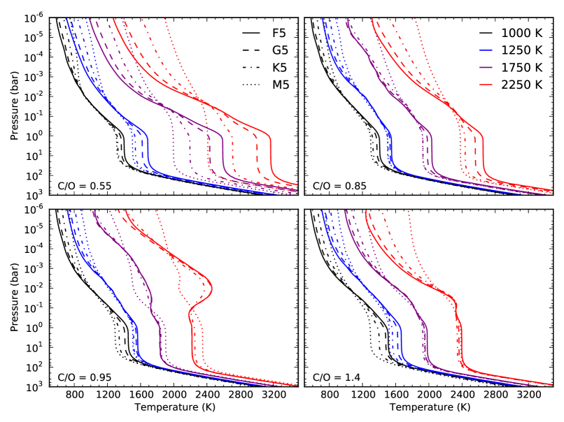
To give a first overview of our of results we show atmospheric -structures of and [Fe/H] = 1 planets for varying host star spectral types (F5, G5, K5, M5) and effective temperature (1000 K, 1250 K, 1750 K, 2250 K) at four different C/O ratios (0.55, 0.85, 0.95, 1.4) in Figure 5.
Some general, expected trends can quite easily be made out from looking at this plot:
-
•
The later the host star spectral type, the more isothermal the atmospheric structure becomes. This is expected because the wavelength range of the received stellar irradiation becomes more and more similar to the wavelength range of the internal planetary radiation field, such that the radiation field absorbed by the gas at the top of the atmosphere is similar to the radiation field absorbed by the gas at the bottom of the atmosphere, hence leading to similar temperatures.
-
•
The -structures with C/O = 0.55 are hotter than the -structures with C/O = 0.85. The main reason for this is that the atmosphere with the lower C/O ratio has, everything else being equal, more oxygen and thus a higher opacity due to a higher H2O abundance. This results in a stronger green house effect, as the excess H2O leads to a less efficient escape of radiation from the atmosphere. In order to radiate away the required amount of energy (set by ) the atmospheres need to be hotter.
Another very striking result is that for C/O ratios close to 1 temperature inversions form in the atmospheres for effective temperatures above 2000 K. In general, they can even occur at effective temperatures as low as 1500 K, see Section V.6. This is interesting, as no extra optical opacity sources such as TiO and VO except for the ones given in Table 1 are being considered. For host stars later than K5 there are no inversions in the planetary atmospheres. This phenomenon will be further studied in Section V.1.1.
V.1.1 Inversions at high C/O ratios
As outlined above, C/O ratios of 1 can lead to inversions in atmospheres with high enough effective temperature if the stellar host is of K spectral type or earlier. The reason for the inversions to occur for these spectral types is that an appreciable amount of stellar flux is received from the star in the optical wavelength regime. This means that the alkali lines, and the pseudo-continuum contribution of the alkali line wings, will become very effective in absorbing the stellar irradiation.
At the same time, close to C/O = 1, most of the oxygen and carbon is locked up in CO, leading to low H2O, CH4 and HCN abundances and opacities.
The combined effect of the effective absorption of the strong irradiation and a decreased ability of the atmospheric gas to cool, because of too little CH4, H2O and HCN leads to the inversion in the atmospheres.
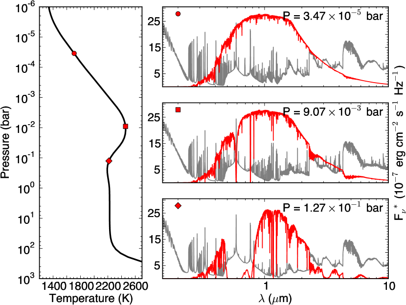
The absorption of the stellar light as a function of depth can be seen in Figure 7, where we plot the -structure of a = 3, [Fe/H] = 1, = 2250 K, C/O = 0.95 atmosphere of a planet in orbit around a G5 star, as well as the local stellar flux at the pressure levels 3.47 10-5, 9.07 10-3 and 1.27 10-1 bar in the atmosphere. Also a plot of the logarithm of the (rescaled) opacity is shown in the Figure for each pressure level. The respective pressure levels are indicated by red points in the -structure.
Figure 7 nicely shows how the alkali pseudo-continuum absorbs the full stellar flux in its wavelength domain at the position of the inversion: At the highest pressure shown in the spectral plots (3.47 10-5 bar) the stellar flux is still completely unaffected by any absorption effects as the atmosphere is still optically thin at all wavelengths (except for right at the core of the alkali lines). At the hottest point in the temperature inversion (at 9.07 10-3 bar) one can see that the alkali wings have already started to absorb non-negligible amounts of energy, and just after the inversion (at 1.27 10-1 bar) the stellar flux in the alkali wings has been completely absorbed. Interestingly, the inversions obtained in our calculations due to alkali heating seem to abide by the rule that the tropopause, i.e. the atmospheric layer at minimum temperature just after the inversion, should commonly be found at 0.1 bar for a wide variety of possible atmospheres (Robinson and Catling 2014).
As can be seen in the stellar flux spectrum at the highest pressure the absorption of the stellar light outside of the alkali wings is rather sluggish, showing the importance of the alkali wings in the formation of the inversion.
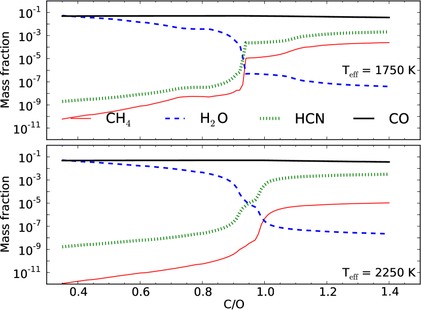
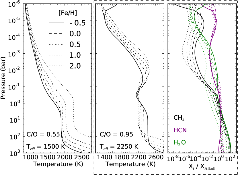
As mentioned above, in a small region of C/O around 1, the atmosphere’s ability to efficiently radiate away the absorbed stellar light decreases due to the involved chemistry. This can be understood by looking at Figure 7, which shows the CH4, H2O, HCN and CO mass fractions in a = 3, [Fe/H] = 1 atmosphere of a planet in orbit around a G5 star as a function of C/O at a pressure level of 9.07 10-3 bar, i.e. close to the pressure where the inversion temperature, if an inversion occurs, is maximal. Two cases for planets with = 1750 K and = 2250 K are shown and we carried out 100 self-consistent atmospheric calculations for both cases with C/O going from 0.35 to 1.4 in equidistant steps.
One sees that for the = 2250 K case, at C/O = 0.95, the H2O abundance has already decreased by 4 orders of magnitude when compared to the lowest C/O values, while the CH4 abundance is still more than 2 magnitudes smaller than its highest abundance at the highest C/O values. Further, HCN has not yet risen to a high enough abundance to take over the cooling. The C/O = 0.95 point at = 2250 K thus is very close to the aforementioned point of minimum IR opacity, leading to the inversions seen in our results for all host spectral types except M5. For higher C/O ratios the IR opacity and the atmosphere’s ability to cool increases, such that no inversions are observed anymore, mainly because HCN takes over the cooling.
For the particular case of = 1750 K in Figure 5 the situation must be different, as there is no inversion present in the atmosphere. The reason for this can be seen in the panel for = 1750 K in Figure 7: for this atmosphere the transition from water-rich to methane-rich atmospheres occurs much quicker as a function of C/O than it does for the = 2250 case. The methane mass fraction jumps from 10-8 to 10-5 at C/O = 0.93 and the HCN mass fraction jumps from 10-6 to 10-4 and no extended region of low water, methane and HCN abundance is seen. Further, as this atmosphere is cooler, the overall CH4 content is higher than in the hotter case. This is expected to occur and has been studied before both in equilibrium and disequilibrium chemical networks (see, e.g., Moses et al. 2013), showing that CH4 becomes less abundant as the temperature increases in carbon-rich atmospheres. In conclusion, this atmosphere can cool more efficiently.
V.1.2 Inversions and line list completeness for HCN and C2H2
We want to issue a word of caution regarding the cooling efficiency of atmospheres. At high temperatures for C/O 1 and 1750 K we find that HCN is more abundant than CH4. It is therefore very important to use HCN line lists which are as complete as possible. In fact we found that if we use HCN from the HITRAN database, which is made for low atmospheric temperatures, we got strong inversions occurring even for C/O 1 if the effective temperatures were high.
Only once we switched to the ExoMol line list for HCN we got the results presented in this paper, where inversions only occur for C/O 1. The ExoMol line list is much more complete for HCN, containing many more lines. The line list is made specifically for high temperatures, optimized for temperatures up to 3000 K and compares well to a high temperature laboratory measurement made at = 1370 K (Barber et al. 2014).777More comparisons are not possible as there are not many high temperature measurements for this molecule. This allows the atmospheres to cool more efficiently, making the inversions go away in many cases.

Likewise, we want to stress that we use the HITRAN line list for the C2H2 molecule, as an ExoMol version is not available. C2H2 is quite common in our results for C/O 1 in the cases where HCN is common as well. This suggests that the atmospheres ability to cool might be further enhanced if high temperature line lists for C2H2 were to be considered.
V.2. Host star dependance of the atmospheres
V.2.1 Spectra
As described in Section V.1 planets orbiting increasingly cooler host stars will approach an increasingly isothermal atmospheric structure, because the spectral energy distribution of the insolation becomes more and more comparable to the SED of the planetary radiation field.
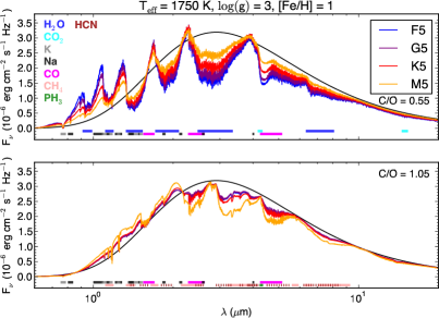
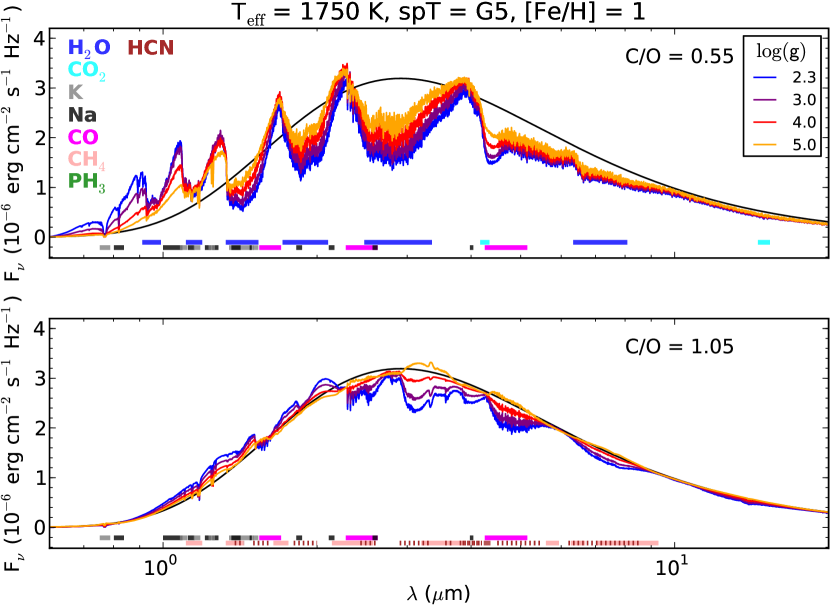
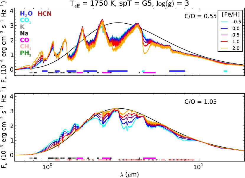
We show the emission spectra of atmospheres with varying host star spectral type for a planet with = 1750 K, = 3, [Fe/H] = 1 for two different C/O ratios (0.55, 1.05) in Figure 8. We indicate the positions of absorption features of H2O, CO2, K, Na, CO, CH4, PH 3 and HCN in the plots. For the atmospheres with C/O = 0.55 the emission spectra clearly become more blackbody-like as the host star gets cooler: the excess emission (with respect to the blackbody curve at 1750 K) of the atmospheres for 1.3 m decreases for cooler host stars. Furthermore the molecular absorption bands in the emission spectra start to get shallower. As expected for a C/O ratio 1, the spectra are clearly water-dominated.
For the atmospheres with C/O = 1.05 the situation is somewhat different. First, the atmospheres are clearly carbon-dominated, showing strong HCN features. Moreover, the latest type host star (M5) causes the least isothermal planetary spectrum, while all earlier type host stars result in a much more isothermal atmospheric structure and, therefore, spectra. This is the contrary of what we saw for the C/O = 0.55 atmosphere, now host stars of an earlier type are making the planetary spectra more isothermal. This is merely the spectral consequence of early type host stars creating inversions or isothermal atmospheres for planets with C/O 1, which we explained in Section V.1.1. As the M5 star is not able to heat the atmosphere enough due to a lack of energy in the optical wavelengths the corresponding -structure and spectra are less isothermal. The -structures producing the spectra shown here for C/O = 1.05 do not have inversions, they are just more isothermal due to the heating. As we will see in Section V.7, atmospheres at = 1750 K can, in general, exhibit inversions.
V.3. dependence of the atmospheres
V.3.1 -structures
The behavior of the -structures as a function of is studied in Figure 10. If one considers gray opacities which are constant as a function of and and assumes hydrostatic equilibrium one obtains the following simple relation between the optical depth and the pressure
| (7) |
where is the gray opacity and g is the gravitational acceleration (taken to be constant). In this case, changing the gravitational acceleration will conserve the temperature structure as a function of , as is the effective spatial coordinate for the radiation field. The mapping from to , however, will change, resulting in locations of a given optical depth and temperature to move to larger pressure values when is increased. This is equivalent to saying that the location of the planetary atmospheric photosphere moves in terms of pressure if the surface gravity is changed.
Thus, when plotting the -structures as a function of planetary gravitational acceleration, as can be seen in Figure 10, one notices that at higher the temperature structure appears to be shifted to larger pressures when comparing to cases with lower . For demonstration purposes we show the -structures up to 10-14 bar. Note, however, that we only calculate the opacities down to pressures of 10-6 bar and adopt the 10-6 bar values at all smaller pressures, i.e. . The -structures for pressures below 10-6 bar are not necessarily unphysical, however (see Section IV.3 for a discussion). The “highest altitude inversion” visible in this plot for pressures much smaller than 10-6 bar is due to the heating by the alkali line cores.
In the top right panel of Figure 10 we show the -structures once more. In this case we have re-scaled the pressures in -structures with higher than 2.3 (which is the lowest value we consider) with . To first order, his should counterbalance the pressure shift of the temperature structure induced by gravity when compared to the = 2.3 case. However, as the opacities are non-gray and varying vertically we expect differences. Nonetheless, the resulting -structures lie on top of each other quite well.
When comparing in greater detail one notices that the deep isothermal regions (at 1-100 bars) are at higher temperatures for lower . Here the pressure dependence of the opacity comes into play: for lower values the stellar light is absorbed at lower pressures, where the atomic and molecular lines are less broadened. This results in the stellar light being able to penetrate deeper in terms of rescaled pressure when comparing to high atmospheres. This means that more stellar light reaches regions of the atmosphere which are optically thick in the near-infrared, which does, in turn, heat up the atmosphere deep in these IR optically thick regions.
In the middle and bottom panel on the right side of Figure 10 we show the fraction of the absorbed stellar flux with respect to the stellar flux at the top of the atmosphere. The middle panel shows this fraction as a function of pressure, the bottom panel shows this fraction as a function of rescaled pressure. One sees that the stellar light is able to penetrate deeper in terms of rescaled pressure in the case of low .
In Figure 10 we have shown an oxygen-dominated atmosphere, where the abundance of the main coolant and absorber, H2O, is roughly independent of pressure. For carbon rich atmospheres the pressure dependent abundances of H2O, CH4 and HCN might play a role in addition to the pressure shift of the temperature structures.
In order to test that our above observations for the oxygen rich atmosphere are not caused by pressure and temperature dependent chemistry effects, we calculated self-consistent structures with vertically constant abundances of molecules and varied the surface gravity.
We found the same behavior of the structures as described above, verifying that the pressure dependent line wing strengths are responsible.
V.3.2 Spectra
In Figure 10 we show the emission spectra of atmospheres with varying surface gravity for a planet with = 1750 K, and [Fe/H] = 1 in orbit around a G5 host star, again for two different C/O ratios (0.55, 1.05). As mentioned above, a variation in the surface gravity rescales the temperatures profiles in terms of pressure. We also found that the deep isothermal regions are hotter for the lower surface gravity cases, because the insolation can probe deeper into the atmosphere. In the pressure rescaled -structures (see upper right panel of Figure 10) one can see that above the isothermal region the atmospheres of planets with higher surface gravity are hotter for a given rescaled pressure: The photosphere is located at higher pressures for a higher surface gravity. It is therefore less transparent, due to the line wing pressure broadening. In order to radiate away the required amount of flux the temperature therefore needs to be higher. The flux in the absorption features then originates in hotter regions, making the absorption troughs shallower in the C/O = 0.55 case. This behavior was verified by the atmospheric structures with vertically constant molecular abundances as well.
In the C/O = 1.05 case the same behavior can be seen, except for the atmospheres with the highest , which shows emission features. Here the stellar light is absorbed over narrower and higher rescaled pressure ranges because the alkali line wings are much broader (the light is absorbed at higher actual pressure). The atmospheric cooling ability, however, is largely independent of pressure, because the emission of light depends on the Planck opacity and , if the pressure dependence of the chemistry is omitted. This causes the atmosphere at highest to develop an inversion.
V.4. Metallicity dependence of the atmospheres
V.4.1 -structures
The influence of the metallicity on the -structures at low C/O ratios is as one would expect: An increased [Fe/H] value in atmospheres leads to higher temperatures in the deep isothermal part of the atmosphere in the cases where no inversions are observed: the temperature structure is scaled to lower pressures as the metallicity increases, as a higher optical depth is reached earlier in the atmosphere. The stellar light can penetrate deeper than suggested by a simple pressure scaling, however: the pressure dependent line wings are weaker (as the atmospheric structures shift to smaller pressures for higher metallicities). This increases the temperature of the atmospheres in the deep isothermal regions at 1-100 bars (see left panel of Figure 12), just like it did for low surface gravities studied in Section V.3. Similar to the test carried out for varying surface gravities in Section V.3 we calculated test atmospheres with vertically constant molecular abundances, scaling the abundances by different factors for different structures, mimicking variations in metallicity without having to deal with effects introduced by chemistry. These calculations showed the same behavior as the nominal calculations when varying the metallicity.
In the case of -structures with C/O , which have inversions, the inversion temperature increases and the region directly beneath (i.e. at higher pressure) the inversions has a lower temperature if the metallicity increases (see middle panel of Figure 12). It is, at first, not evident why this should happen, because if all the metal atomic abundances scale with 10[Fe/H] one would expect the same for the resulting molecular abundances and opacities, and therefore the heating vs. cooling ability of the atmosphere should stay the same. This interpretation is consistent with the analytical double-gray atmospheric models as published, e.g., by Guillot (2010); Hansen (2008); Thomas and Stamnes (2002), where the inversion temperature should stay constant unless the ratio
| (8) |
changes, where and are the mean opacities in the visual and IR wavelengths in the atmosphere. The behavior we see in the atmospheres suggests that
| (9) |
which should only be possible if and (and the molecular abundances giving rise to these opacitites) do not just simply scale linearly with metallicity. In order to test this we checked the abundances of the major absorbers and emitters as a function of metallicity throughout the atmospheres for the -structures shown in the middle panel of Figure 12. Indeed we found that the ratios of mass fractions and decreased when the metallicity was increased (see right panel of Figure 12). increases, at the relevant temperatures already being the dominant carbon opacity carrier. However, the increase in is apparently not enough to act as a counterweight compensating the loss of infrared opacity due to the lower . This leads to less efficient cooling as [Fe/H] increases. This abundance change is likely caused by the pressure dependence of the chemistry, as higher metallicities shift the temperature structure to smaller pressures, where, for carbon-dominated atmospheres, CH4 and H2O are less abundant, while the HCN abundance increases.
V.4.2 Spectra
Analogous to the case an increase in metallicity (and thus opacity) can be regarded as a similar pressure rescaling, as we found for a gray atmosphere with vertically constant opacity that . As is in the numerator, atmospheric structures with increased metallicity should behave similarly to structures with decreased surface gravity, featuring a higher temperature in their isothermal regions, but a lower temperature (as a function of rescaled pressure) in the higher atmosphere: Because the photosphere will be located at smaller pressures (in actual, non-rescaled pressure) for an increased metallicity, the line wings will be less strong (less pressure broadening). The atmosphere is therefore more transparent and cools better. In order to radiate away the imposed flux, the temperature in this more transparent photosphere needs thus to be decreased. The minima in the spectrum, stemming from the opacity maxima, i.e. the line’s Gauss-cores, will originate from the same region in terms of rescaled pressure. As these pressures are now at a lower temperature, this leads to deeper absorption troughs in the spectra. This can be seen in the upper panel of Figure 12 and was confirmed by the vertically constant molecular abundance calculations as well, when rescaling the abundances as described above. In summary, more pronounced absorption troughs can mean either a lower surface gravity or a higher metallicity (see figures 12 and 10).
In the C/O = 1.05 case we can again draw on our studies of the -structures: we saw that for atmospheres with inversions, due to the chemistry involved, the cooling ability of the atmospheres relative to the heating by the alkalis decreases if the metallicity is increased (see middle and right panel of Figure 12). The spectra shown in the lower panel of Figure 12, although they do not exhibit inversions, are consistent with these observations, showing absorption spectra which become more and more isothermal as the metallicity is increased.
V.5. Low temperature atmospheres ( K)
At low enough temperatures ( K) HCN does not yet play a significant role for the atmospheric spectra. Additionally the left pointing arrow of the chemical reaction in equation (6) can still be of importance, meaning that H2O and CH4 are significant carriers of C and O atoms. It is important to note, however, that the chemical equilibrium abundances are not only temperature, but also pressure dependent:
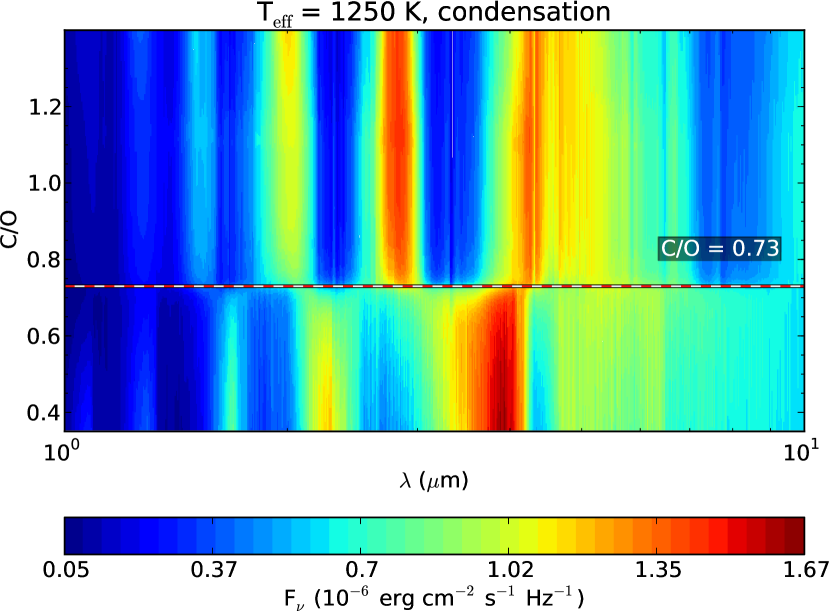
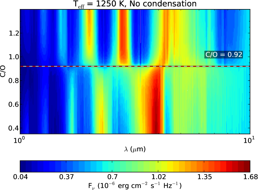
at low temperatures and high pressures CH4 will be abundant also in an oxygen-rich atmosphere, while H2O will be abundant in carbon-rich atmospheres. At low temperatures and low pressures CO will become increasingly important, such that the oxygen-rich atmospheres do not contain a lot of methane and the carbon rich ones do not contain a lot of water.
As seen in the above discussions, [Fe/H] and can strongly influence to which pressure levels the optical depth-dependent temperature structure will be be scaled, as for a gray atmosphere it would hold that . Therefore, low metallicity atmospheres (causing a small ) at high surface gravities cause the temperature structure to be scaled to high pressures. In Figure 13 we show emission spectra of planets with = 1000 K in orbit around a G5 star. The spectra are shown for C/O = 0.55 and 1.12 in the upper subpanels. Furthermore we indicate the positions of absorption features of H2O, CO2, K, Na, CO, CH4 and PH3 in the plots. The left panel shows the emission spectra for planets with = 4, [Fe/H] = -0.5. This means that here the surface gravity is high and the metallicity is low, causing the temperature structures to be scaled to high pressures. The right panel shows planets with = 2.3, [Fe/H] = 2, i.e. with low surface gravities and high metallicities, leading to temperature structures to be scaled to low pressures. In the lower subpanels we show color maps of emission spectra as a function of wavelength (-axis) and C/O ratio (-axis).
In the right upper subpanel, one sees that the two spectra are very different, showing either water or methane features for the atmospheres with C/O =0.5 or 1.12, respectively. As described above, this is expected, corresponding to a low pressure scaling of the temperature structure and due to the pressure dependence of the CO–CH4–H2O chemistry. In the lower right subpanel there is an overall shift from H2O to CH4 dominated spectra at C/O 0.73.
As expected, in the left panel there is only little difference between the oxygen-rich and carbon-rich case. Further, the lower left subpanel does not show any transition between a water- and methane-dominated atmosphere, as both molecules are present in the atmospheres at all C/O ratios. Once more, this is expected, as in this case, i.e. for low metallicity and high the photosphere of the atmosphere is scaled to high pressures, where the chemistry dictates that CO is not the major carbon and oxygen carrier, but instead CH4 and H2O dominate, at least at the low atmospheric temperatures considered here. Therefore, although the CH4/H2O number ratio may change as a function of C/O, this change is not sufficient to affect the spectrum significantly.
Therefore, the spectral appearance of a planet is not only given by the C/O ratio and the effective temperature but also by a factor
| (10) |
which is a measure for the optical depth – pressure mapping in the atmospheres and gives insight to which pressure levels a given atmospheric temperature profile is scaled. We found that transitions between water- and methane rich atmospheres occur at or for = 1000 K. For = 1250 K we found that , indicating that a transition between water and methane dominated spectra should always be expected at these temperatures. However, values of close to this threshold should always exhibit some methane or water features, even if the atmosphere is water or methane dominated, respectively.
V.5.1 C/O dependence with and without condensation
For atmospheres with effective temperatures 1750 K, the spectrally active parts of the atmosphere have temperatures low enough for the condensation of MgSiO3 (for the temperature dependent saturation vapor pressure of MgSiO3 see, e.g., Ackerman and Marley 2001).
Condensation of O in MgSiO3 does not have a too strong effect on the spectra in the sense that they are either water or methane dominated at high enough temperatures, i.e. 1000 K. It does shift the C/O ratio-dependent transition between the 2 cases, however, as we detail below. Note that we do not include cloud opacities yet, so the presence of MgSiO3 grains will not affect the radiation field.
For atmospheres with C/O values in the vicinity to, but less than 1, the condensation of MgSiO3 decreases the amount of oxygen available to form CO and H2O considerably.
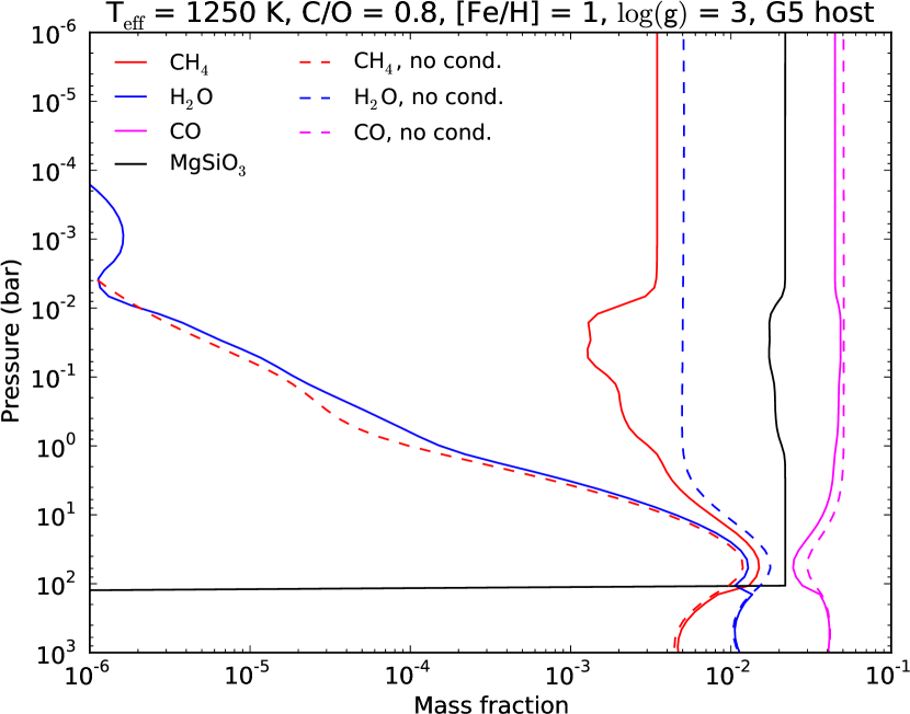
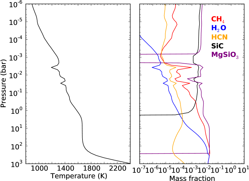
In turn the H2O features in the spectra will weaken and CH4 can form in noticeably higher abundances as C atoms are more available due to the lower amount of CO being formed.
This results in shifting the transition from H2O to CH4/HCN dominated spectra from C/O = 0.92, which we obtain for atmospheres with 1750 K, to C/O = 0.73 which we obtain for 1750 K, as we described in the previous section.
In order to test this condensation dependance further we carried out atmospheric calculations at = 1250 K, neglecting the effect of condensation.
A comparison of the resulting emission spectra as a function of C/O for both cases ( = 1250 K, with and without considering condensation) can be seen in Figure 14. We calculated atmospheres with C/O ratios spaced equidistantly between 0.35 and 1.4 using 100 grid points for both cases. The difference in location for the shift from water to methane dominated spectra, moving from C/O = 0.73 (condensation) to C/O = 0.92 (no condensation), is very prominent in these plots.
To further verify this finding we plot the mass fractions of H2O, CH4, CO and MgSiO3 in Figure 16 for a planetary atmosphere with = 1250 K, C/O = 0.8, = 3, [Fe/H] = 1 in orbit around a G5 star. The C/O value is chosen such that the atmosphere is water dominated in the model neglecting condensation, but it is methane dominated in our nominal atmospheric model, which includes condensation.
One clearly sees that for high pressures, where the temperatures are too high for MgSiO3 to condense, the abundances of H2O, CH4 and CO for both models are nearly identical. The small differences are due to differences in the -structures found for the 2 chemical models. For pressures smaller than 10-2 bar, however, MgSiO3 starts to condense, noticeably decreasing the CO and H2O abundances. CH4 becomes much more abundant than H2O, which is in contrast to the behavior of the model without condensation, where H2O stays more abundant than CH4 throughout the atmosphere.
We therefore conclude that the transition from water- to methane-rich spectra may happen at C/O ratios considerably smaller than 1 if the planetary effective temperature is not too high. Especially for retrieval analyses of planetary spectra, which measure the local gas C/O ratio in the spectrally active regions of the atmosphere, the above findings are relevant. If condensation is expected to occur, a result such as “C/O 1”, due to the absence of methane features, could actually indicate an even lower total (gas + condensates) C/O ratio0.7. If a given atmosphere were enriched in Mg and Si one would expect this effect to be even stronger, shifting the transition between carbon and oxygen rich spectra to even lower C/O ratios.
Finally, we want to remind the reader of the simplifications of our chemistry model, which does neither include settling nor properly accounts for the effects of homogeneous or heterogeneous nucleation (see Section IV.2). Furthermore the absence of quenching in our models might be problematic if the timescales for condensation and chemistry in general are longer than the vertical eddy-diffusion timescales. Nevertheless, similar results have been found with much more sophisticated condensation models: Helling et al. (2014) were able to produce local C/O 1-2 values in the gas phase for an atmosphere with a global C/O = 0.99 due to the condensation of O in dust species. Their model for condensation and cloud formation is much more complete and includes homogeneous and heterogenous nucleation, settling, traces the growth and evaporation of grains, and considers more condensable species than our model.
Given these differences in condensation modeling it will be very important to reinvestigate our findings presented here with more sophisticated cloud models in the future.
V.6. Intermediate temperature atmospheres ( K)
At = 1500 K the transition from oxygen to carbon dominated atmospheres is still at C/O = 0.73 as silicate condensation still takes place. Furthermore, the carbon dominated atmospheres show strong methane features, but HCN features start to emerge as well.
V.6.1 Inversions and kinks at = 1500 K and C/O 1
At = 1500 K and C/O 1 condensation can lead to weak inversions and, occasionally, to kinks in the -structures. For C/O ratios 1 the atmospheres are already carbon dominated.
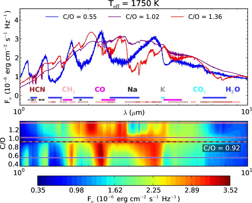
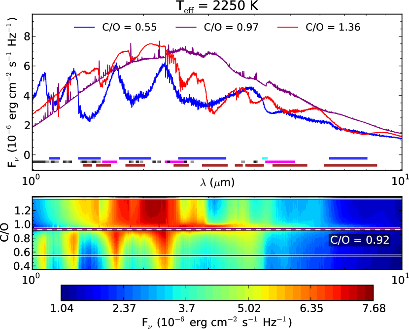
In general, the atmospheres are still too cool to contain enough HCN to efficiently radiate away the absorbed stellar energy, such that H2O and CH4 are the main absorbers and the H2O–CH4–CO chemistry is important. At the intermediate atmospheric temperatures considered here, inversions are likely to occur because of the condensation of SiC. This results in a lower abundance of SiO, as less Si is available. The O atoms which are not bound in SiO anymore form more CO and thus decrease the C budget available to form CH4, therefore decreasing the atmosphere’s ability to cool. This effect can be further enhanced by the evaporation of MgSiO3 in the inversion regions, which frees additional O to be put into CO, subsequently locking up more C atoms. As for the atmospheres which have inversions at C/O 1 at higher effective temperatures, the inversions vanish for higher C/O ratios 1: less oxygen is present to form CO in the first place. Therefore more CH4 can be formed.
At = 1500 K kinks in the PT-structure can occur when condensation of MgSiO3 and the associated locking up
of oxygen causes the cooling to become more strongly methane-dominated in a certain layer,
whereas there is less methane present to cool in an adjacent, hotter layer in which there is less MgSiO3
and more oxygen is available in the gas phase to form CO and water, locking up carbon and decreasing the methane abundance.
The cooling ability of the methane-deprived layers is lower, leading to a strong temperature change from one layer to the next.
Such kinks depend on the choice of the grid spacing and
cell locations, such that they should not be treated as real physical phenomena but rather numerical artifacts.
The corresponding structure files have been flagged with “_kink”.
As inversions due to alkali heating and a low cooling ability are in general not seen in our results for M5 host stars, the kinks and inversions are not present for planets with M5 hosts.
In Figure 16 we show an example for the kinks which are caused by the condensation. One clearly sees that the kinks in the -structures going to hotter temperatures are caused by the (partial) evaporation of MgSiO3, reducing the amounts of coolants such as CH4 and HCN.
V.7. High temperature atmospheres ( K)
At high temperatures condensation processes do not play an important role anymore.
Therefore, the transition between water and carbon-dominated spectra shifts from C/O = 0.73
to 0.92. Furthermore the carbon-rich atmospheres become more and more HCN dominated
and CH4 becomes less and less important as the temperature increases.
As mentioned before, the chemistry is not only temperature but also pressure dependent,
favoring HCN over CH4 at high temperatures and low pressures.
= 1750 K
At K, we find that the higher the -factor
(see Equation 10) of an atmosphere is, the more HCN dominates the spectrum.
Methane features are visible for all s, however.
Due to the chemistry, a low -factor allows for some presence of water in the carbon-rich
atmospheres. Thus at low s we find a weak water absorption signature imprinted
on the rather opacity free region extending from 2.4-3 m, which is bracketed by
two CH4 features.
Because of the strong stellar irradiation the atmospheric structures at C/O
1 become either more isothermal or exhibit inversions.
We show spectra of atmospheres with = 1750 K and varying C/O ratios in the left panel of
Figure 17.
= 2000 K
At even higher temperatures HCN becomes more dominant.
Inversions at C/O 1 predominantly form for low -2.5 (or -2) in these atmospheres.
For the larger values the methane features fade away.
= 2250 K
For = 2250 K the atmospheres with C/O 1 are strongly HCN dominated.
Only for low values weak methane features are present.
Furthermore more or less all atmospheres with C/O 1 have inversions if the spectral type of the
host star is K or earlier.
We show spectra of atmospheres with = 2250 K and varying C/O ratios in the right panel of
Figure 17.
= 2500 K
For = 2500 K the atmospheres with C/O 1 are completely HCN dominated,
and the methane features have vanished.
All atmospheres with C/O 1 have inversions if the spectral type of the
host star is K or earlier.
VI. Summary and conclusion
In this work we present a systematic parameter study of hot jupiter atmospheres. In addition to “classical” grid parameters such as metallicity, effective temperature and surface gravity we study the effects of the atmospheric C/O ratio as well as the host star spectral type. We summarize the key findings of our study in Figure 18 and in the text below.
-
•
At low effective temperatures ( 1500 K) the atmospheres can be either water or methane dominated, but not always: if is small, the spectra at 1000 K are quite similar, showing both strong water and methane features. The optical depth (and hence temperature) versus pressure profile scales approximately with . Hence, a given optical depth (temperature) is reached at high pressure when beta is low and vice versa. We want to remind the reader, however, that we neglect quenching, which could potentially alter the methane and water mixing ratios. For high pressures and low temperatures CH4 and H2O co-exist as the dominant oxygen and carbon opacity carriers, and are both visible in the spectrum. At values above -4 to -3.5, the atmospheres are either water- or methane-dominated at = 1000 K. For atmospheres with = 1250 K the spectra look similar only for the highest surface gravities ( = 5) and lowest metallicities ([Fe/H] 0), such that these atmospheres should be either water or methane dominated for most planets.
-
•
At 1500 K the condensation of MgSiO3 is a relevant effect at the local atmospheric temperatures. The condensation effectively lowers the amount of oxygen which can be put into CO and H2O, such that more carbon atoms are available to form CH4. As a result the atmospheres start to be methane dominated at C/O = 0.73. For higher temperatures MgSiO3 can no longer condense, shifting the transition from oxygen to carbon dominated spectral signatures to C/O = 0.92.
-
•
For planets with 1500 K and C/O 1 host stars with spectral type earlier than M5 (we consider M5, K5, G5, F5) can lead to temperature inversions in the atmospheres. The reason for this is that under these circumstances all the main coolants of the atmosphere, H2O, HCN, and CH4, are depleted, whereas the absorption of optical radiation by the alkali metals remains highly effective. For = 1500 K the condensation of SiC can sufficiently lower the cooling ability for inversions to develop. At this effective temperature the condensation of MgSiO3 can lead to kinks and numerical instabilities in the solutions for the -structure. For = 2000 K all atmospheres with -2 to -2.5 will exhibit inversions. For 2250 K all atmospheres with C/O 1 exhibit inversions.
-
•
The lower = [Fe/H] - , the more methane-dominated the spectra are at C/O ratios 1. At higher temperature and/or higher values, such planets have HCN-dominated spectra. In general we show the dominant absorbers as a function of temperature and C/O ratio in Figure 18.
-
•
The host star spectral type is an important factor for the spectral appearance of the atmosphere. For planets with C/O 1 host stars of spectral type K or earlier can give rise to inversions if they are at small enough distances, whereas for M-type host stars inversions do not occur. Further, the later the host star spectral type, the more isothermal the planetary atmospheres become (if the C/O ratio is not 1). This is because SED of the stellar irradiation becomes increasingly similar to the planetary radiation field.
-
•
Planetary metallicity and surface gravity determine the location of the planetary photosphere. High surface gravities or low metallicities will shift it to larger pressures, whereas low surface gravities or high metallicities shift it to low pressures. As the molecular and atomic line wing strength scales approximately linearly with pressure, for photospheres at low pressures the flux is originating at somewhat deeper layers (in terms of optical thickness), leading to somewhat cooler atmospheric temperatures and hence deeper absorption troughs. The deep isothermal temperature increases in these cases, as the insolation can probe deeper into the atmospheres. Similar results for the surface gravity dependence of the absorption troughs have also been reported in Sudarsky et al. (2003).
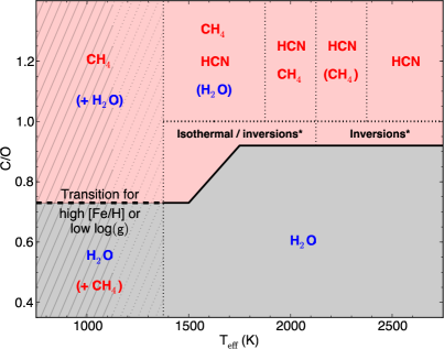
It is interesting to see that at low temperatures the strength of methane or water features does not only depend on the C/O ratio, but also on the pressure level of the photosphere, which can be quantified using the the factor. For higher temperatures the factor plays a role as well, as it determines whether CH4 or HCN dominates the spectra of carbon-rich atmospheres. Also the occurrence of an inversion at C/O 1 can be tied to the factor, at least for the atmospheres with 2000 K. Therefore the factor can be used as a third dimension to characterize the spectral appearance of an exoplanet, in addition to the effective temperature and the C/O ratio.
Moreover, the fact that the transition from water to methane rich spectra shifts due to the condensation of silicates, which lock up oxygen, is important when carrying out retrieval analyses of planetary atmospheres. The C/O ratio is often measured by taking into account the abundances of only the gaseous carbon and oxygen carrying molecules. This can potentially overestimate the total (gas + condensates) C/O ratio. It is important to note that our current condensation model is simplified, assuming instantaneous condensation once the saturation vapor pressure is exceeded and no settling or mixing of the cloud particles. It will therefore be very important to investigate this effect in the future in greater detail, using a more sophisticated condensation model.
The fact that inversions can potentially occur at C/O 1 is interesting, as we did not require any additional absorbers such as TiO and VO, the absorption of stellar light by the alkali atoms is sufficient. To further study the inversions it is necessary to obtain molecular line lists as complete as possible as their occurrence is very strongly dependent on the atmospheric cooling ability.
The grid of atmospheres presented in this work is made publicly available and can be found at the CDS.
Appendix A A fast method to calculate opacities from line lists
If one wants to calculate the line opacities of a given molecule on a given grid of wave number points one must, in principle, and if no line truncation is applied, calculate the line profile of every line at every wave number grid point. Even if one precomputes the opacities and tabulates them for later use it can still take a long time to calculate the total molecular cross-section as the calculations need to be carried out at high resolution. Using a fiducial resolution of and considering a species with of the order of lines one easily ends up with line profile evaluations at just one given pressure and temperature.
To speed up the calculations of line opacities the method explained below was developed and used for our opacity database calculations. In essence we calculate the line cores of every line at high resolution, while calculating the line wings far from the line core on a much coarser grid. Once the contribution of all the lines to the coarse grid has been calculated it is interpolated back to the fine grid. In detail we proceed as follows:
Divide the total wave number grid into subgrids of 10,000 grid points. Then start to go through all these subgrids, which will be indexed by :
-
•
Calculate all line opacities of lines that are lying within the subgrid at all of its 10,000 wave number grid points.
-
•
Then iterate over all other subgrids (which are indexed by n). For the external lines in a given external subgrid with do the following:
-
1.
If (i.e. Gaussian width larger than Lorentz width): If the distance of the line to the subgrid border of is smaller than , where is a factor that needs to be specified, then this line gets calculated at all of ’s 10,000 subgrid points. Otherwise go to step 2.
-
2.
If or the distance to the subgrid border of is larger than :
Consider the Lorentzprofile . Far away from the line center its functional form is roughly . The relative deviation from this form is(A1) I.e., if we want a maximum deviation of less than from the above form, then we need that
(A2) If this is not fulfilled, then the line opacity is just calculated at all of ’s 10,000 subgrid points. It it is fulfilled go to step 3.
-
3.
For all lines within a given external subgrid that fulfill the above inequation: Calculate the line strengths on a coarse subgrid of 10 points within the original subgrid and add the results for all these lines up, then interpolate back to the 10,000 original grid points in , using a powerlaw interpolation and a coordinate transformation (a simple shift).
-
4.
Move on to the next external subgrid , go back to step 1.
-
1.
-
•
Move on to the next subgrid .
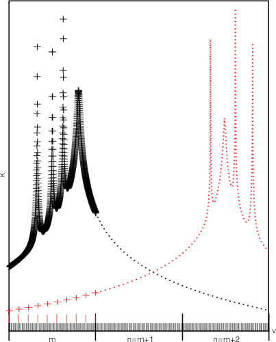
The reason to interpolate back to the 10,000 subgrid points of for all external subgrids seperatly is the following.
For a single line, far away from its line center, the line shape is roughly
| (A3) |
Thus for all transitions of strength which are contained in a subgrid the total continuum line strength (i.e. the wing strength of a line far away from its line core) will be
| (A4) |
Seen from subgrid all lines within a given subgrid have roughly the same line center position (namely within subgrid ), thus one can do the coordinate transformation , where is the position of subgrid (e.g. the wave number at its center). This would yield
| (A5) |
Thus for every subgrid one can do a coordinate transformation to and finds that the coarse 10-point subgrid continuum of subgrid seen in subgrid should roughly behave like a powerlaw function with a powerlaw slope of . This explains why a powerlaw interpolation in the coordinate is the best thing to do when interpolating the coarse continuum of the lines in subgrid n back to the fine grid in subgrid . It should also be stressed that it is better to do an interpolation that finds the effective powerlaw slope, rather than taking it to be and using , as there will be slight deviations from this powerlaw shape, as one knows that the line centers in subgrid are close to , but not exactly at . An interpolation will mitigate this problem by finding a slightly different powerlaw shape and an overall coefficient for the function that slightly deviates from . For continua produced by lines that are outside of the total grid we use a linear interpolation, as we don’t actually check where these lines are sitting. In Figure 19 one can see a schematic drawing explaining the acceleration method introduced in this section.
All our opacity calculations were carried out using the accelerated method on a grid with a point spacing of . Additionally we performed a “classic” calculation on a reduced grid constructed by using every 1,000th fiducial wave number grid point. On this reduced grid we did not use the aforementioned acceleration method but calculated every line contribution at every wave number point. The high resolution result of the accelerated method was only kept if the maximum relative deviation at the points coinciding with the 1,000 times coarser test grid was smaller than 1 %. If it was bigger, was increased and was decreased and the calculation was repeated.
Appendix B Correlated-k: Going from to
In the following we describe our method of combining the opacity tables of multiple species. Furthermore its implementation at different grid resolutions is explained. For a general review of the correlated-k method see, e.g., Marley and Robinson (2014).
B.1. The “classical” case
The commonly utilized method to combine the k-tables of multiple species is numerically quite expensive, as it is of order , where is the number of grid points used in -space ( is the cumulative opacity distribution function, see below) and is the number of species. In this traditional method, the computation of the total opacity works as follows: In a spectral region of the frequency interval the transmission of light through a layer of thickness which contains 2 spectrally active species is
| (B1) |
where and are the mass fractions and opacities of the two species, is the gravitational acceleration in the atmosphere and is the atmospheric layer thickness in units of pressure. For simplicity it is assumed that and are constant within the atmospheric layer. If one assumes the opacities of species 1 and 2 to be uncorrelated, i.e.
| (B2) |
where are the opacity distribution functions, one can rewrite the transmission as
| (B3) |
An opacity distribution function within a frequency interval is defined by being the fraction of the opacity values within which lie between and . Going from frequency space to -space, where g is the cumulative opacity distribution function (), and approximating the integrals with sums yields
| (B4) |
The combined total k-table of species 1 and 2 therefore has the opacity values
| (B5) |
which have to be weighted with
| (B6) |
As is commonly pointed out the number of operations that need to be carried out in order to combine the k-tables of multiple species is thus , which can make the consideration of multiple species computationally expensive (see, e.g., Marley and Robinson 2014; Lacis and Oinas 1991).
B.2. The case
B.2.1 Algorithm used at a bin size of (R1000 method)
In order to combine the individual k-tables of all species of interest for finding the total k-table of an atmospheric layer we use a method that is computationally less expensive. Similarly to the “classical” approach, the method makes use of the assumption that the opacities are not correlated. The main idea is to iteratively combine the opacities of two species: The opacity of a real species and the effective opacity of a “help”-species. If the opacities of all species are uncorrelated, then the combined opacity of two species is not correlated with the opacity of any other remaining species. Furthermore the combined opacity of the two combined species can be treated as belonging to a new single species, which is the “help”-species.
We thus proceed in the following way: For every species, within every bin, we save the opacity distribution on a grid of 30 points. The 30-point grid consists of two 15-point Gaussian grids ranging from 0 to 0.9 and from 0.9 to 1, respectively.888 This is not the same grid on which the radiative transport will be carried out on. The radiative transport grid consists of 20 points. The 30-point Gaussian grid is only used for the combination of the k-tables. Now, when starting to construct the total opacity, the first two species 1 and 2 get combined according to equations (B5) and (B6). This results in new values which need to be sorted by size. Using the cumulative sum of the associated weights , where and are the respective Gauss-grid weights, we interpolate the result back to the original 30-point Gauss-grid. This newly obtained opacity is then iteratively combined with the remaining species’ opacities and results in the final opacity distribution . In a procedural notation the method can thus be described as
Total opacity = X_1 * kappa(g) of species 1

For all remaining species (i = 2 to N_sp) {

  Total opacity =   combine(Total opacity,
       X_i*kappa(g) of species i)

  re-bin Total opacity to nominal g-grid

}
For notational convenience the method for combining the opacities as introduced in this section will be called “R1000 method” in the following sections. The number of points used for combining two species’ opacities will be called . As explained in this section, the nominal value of when working at a resolution of is .
B.2.2 Algorithm used at a bin size of and
In order to correctly describe the opacity distributions at small many -grid points would need to be used, as especially at low pressures the opacity tables tend to be very sharply peaked at values very close to 1. Therefore the R1000 method would become numerically inefficient and cannot be used.
However, once more the idea is to combine two species iteratively in order to obtain the total opacity. Moreover, we again make use of the assumption that the opacities are not correlated. In the and cases the spectral bins are 100 or 20 times larger than in the case. They therefore include many lines, and the assumption of uncorrelatedness should be valid to an even higher degree than in the case.
The idea to obtain the total opacity is the following: In principle the combination of two species could be accomplished by randomly sampling the 2 individual opacity distributions and taking the sum of the sampled values as a set of the combined opacity. In a numerically simplified version one could discretize the opacity distributions by providing a pre-sampled set of opacity values and their corresponding weights .
The random sampling could then be approximated by randomly drawing values from the opacity sets of each species and adding them, taking into account their weights at the same time. If one would sample continuous values from a distribution, it is possible to sample values from within a given interval multiple times. Thus, if a discretized opacity value has been drawn from the opacity set it must in principle not be excluded from being drawn in any of the next sampling steps.
The discretization is carried out in the following way in our method: For every species we divide the table of every species into two sets. The first set contains values with . The -coordinates are located at the centers of grid cells defined by grid borders spaced equidistantly between and . The second set contains values with . These values are located at the centers of grid cells defined by grid borders spaced equidistantly between and . We chose and . The values of a species with will in the following be called and the values with will be called . Additionally, for every species, we save the lowest and highest opacity value within the frequency bin, corresponding to the and opacity values. describes the low , continuum properties of the species’ opacity, while describes the high , line core properties of the species’ opacity.
Returning to sampling values from 2 species, the probability of sampling and combining 2 values stemming from the respective -regions is . The probability for combining 2 values from the -region of species 1 and the -region of species 2 is etc…
To speed up sampling, we now assume that once an opacity value of a given species has been drawn, it cannot be drawn again (we will return to the validity of this approach below).
In order to approximate the sampling process of the combined opacity distribution function of two species, we then construct a matrix containing the various possible combinations of and of both species, weighted by how common these combinations would be in a random sampling process of both species’ opacities. When sampling points from species 1 and combining them with sampled points from species 2 the assumption that a given value can not be redrawn allows for a simple shuffling in the sampling process:
| (B7) |
The first column of represents the sampled values of the new combined opacity, the second column gives the weight of each sampled value, similar to the weights in the classical method described in Section B.1. We then sort the lines of the matrix by the values in the first column. After this we construct a vector of length with the entries (starting at )
| (B8) |
and . The second column of is then replaced with . After this, the first column of contains the newly sampled values of the combined opacity of species 1 and 2, the second column contains the corresponding values. Using and the total opacity can then be interpolated to the low- and high- values to yield the final result. The resulting opacity is then ready for being combined with the opacity of the next species. In order to shuffle the opacities we use the Knuth-shuffle algorithm, which is of order .
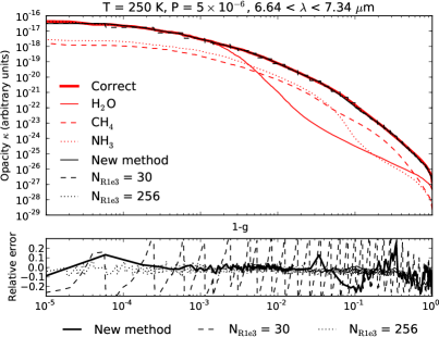
The assumption of not being able to draw a given opacity value more than once is obviously not correct. However, it has been found to not affect the quality of our results. From the above we see that in every combination step one needs to sort values. In the R1000 method we would have the same computational costs when storing opacity points per species, losing resolution when comparing to the points we use in the method introduced here. Furthermore, the results of the R1000 method, at the same computational cost, turn out to be much worse, both when comparing to the actual shape of the wanted total opacity distribution as well as when comparing
| (B9) |
for both methods.999We will need to evaluate Eq. (B9) when computing the Planck mean opacity in the temperature calculation. The error of our method is in the range of %, whereas the error of the R1000 method at the same computational cost is in the range of tens of %. Comparing the results of the new method with results of the R1000 method when taking , i.e. the same number of points in both cases, yields slightly better results for the R1000 method. However the numerical costs for the R1000 method are , while they are in the new method presented here. The reason for the R1000 method at the fiducial resolution to fail here is that we consider 20-100 more points per wavelength bin. This requires a higher resolution when trying to resolve the actual opacity distribution function.
In Figure 20 one can see an example calculation from combining the opacities of water, methane and ammonia in the wavelength range going from 6.64 to 7.34 m. The distributions of the individual species are shown in the plot. All species are contributing approximately equally strong to the total opacity in this example and have lines in the wavelength region of interest. Therefore this case represents something like a worst-case scenario, as our method is the most accurate when one species dominates or the other species only contribute via a their line continua. We plot the correct total distribution, obtained when adding the opacities in frequency space first, as well as the results obtained from using the R1000 method and the result from using the new method introduced in this section. The -grid used for the R1000 method was chosen to have values following a distribution in order to trace strong changes in the opacity distributions. One sees that our new method is never worse in accuracy than the R1000 method which even has a little higher computational cost (), and usually has an relative error which is an order of magnitude smaller. The error of the results is an order of magnitude smaller than the result.
Finally we note that our spectral calculations using the above efficient method at do not deviate by more than 5 % (and usually less) in wavelength regions of appreciable flux when comparing to the rebinned line-by-line calculations (see Section II.4.1, Figure 2). This is a deviation commonly stated for correlated-k (see, e.g., Fu and Liou 1992; Lacis and Oinas 1991). The strength of the new method reported here is to be numerically efficient, while conserving the opacity information at a high level of detail.
Appendix C Use of the Variable Eddington Factor method to find the temperature
C.1. Basic equations
For the moment equation based approach of solving for the -structure we first need the equation of radiative transport, neglecting scattering processes for now:
| (C1) |
In our case, the source function is simply the Planck function,
| (C2) |
where .
We now make the plane-parallel assumption, which states that any spatially varying quantity can only vary in the vertical direction . We chose to increase towards the upper layers of the atmosphere. The equation of radiative transport then transforms to
| (C3) |
where and being the angle between the vertical and the direction of the ray. is the polar angle around the -axis. Note that is independent of both and when it is equal to the Planck function.
The zeroth, first and second radiative moments are defined as
| (C4) |
In plane-parallel geometry and rotational symmetry around the -axis (i.e. no -dependence), only the -component of the first moment and only the -component of second moment are unequal to 0 and one can define
| (C5) | ||||
| (C6) |
where the subscript has been omitted. The definition of the three plane-parallel moments then is
| (C7) |
For radiation emanating from a small solid angle (while keeping the -only spatial dependancy) one finds that
| (C8) |
where and being the angle between the vertical vector and the vector pointing in direction . and are, once more, the - and -component of and . If the radiation emanates from a star of radius at distance , where , then
| (C9) |
Integration of Eq. (C3) over the whole solid angle yields
| (C10) |
where we used that the source function is supposed to be the Planck function. Note that this equation holds independently of the fact whether there is a -dependance in the radiation field or not as long as the definition is used. It can thus also be used for the radiation emanating from a small solid angle. Multiplying Eq. (C3) by and integrating over the whole solid angle again yields
| (C11) |
where the isotropy of the Planck function was used. Equations (C7), (C8), (C10) and (C11) are the equations of interest for the task of finding the structure.
C.2. Solution of the -structure problem
The method explained below is based on the method used for protoplanetary disks introduced in Dullemond et al. (2002).
A useful spatial coordinate for the -structure calculation is the pressure , rather than the height : At the top of the atmosphere we have and the starting point of can be chosen arbitrarily. In contrast to the pressure, where we have a well defined value at the top of the atmosphere, namely . Furthermore the use of the pressure instead of some arbitrary height in the atmosphere makes the density drop out of all equations of interest. To eliminate the vertical height from the equations, we use the equation of hydrostatic equilibrium
| (C12) |
where is the density and is the gravitational acceleration, which is taken to be constant throughout the atmosphere. Furthermore we will use that
| (C13) |
where is the monochromatic opacity.
The optical depth then relates to the height as
| (C14) |
This yields
| (C15) |
C.2.1 Incident stellar irradiation
For simplicity we assume the stellar irradiation field to be a black body in this section. In the implemented version of our code we are able to use either a blackbody or an actual stellar spectrum. In the latter case gets replaced with the stellar spectrum appropriate for a main sequence star at a given effective temperature.
First we start with the stellar light shining at the atmosphere of the planet. The stellar effective temperature shall be . If one then defines the irradiation temperature as
| (C16) |
then equations (C8) and (C9), together with yield for the frequency integrated first moment in z- direction that
| (C17) |
where it was used that
| (C18) |
The negative sign implies that the radiation enters the planet, rather than leaving it. Furthermore we make the so-called two stream approximation, assuming that the stellar irradiation is in the optical wavelengths, while the radiation field inside the planet is in the IR-wavelengths due to the lower temperature of the planetary atmosphere. Any emission processes in the atmosphere at the stellar irradiation wavelengths are thus neglected and the corresponding source term in the equations of interest are neglected, leading to
| (C19) |
and
| (C20) |
where equations (C10), (C11) and (C14) were used. Using Eq. (C8) to see that yields
| (C21) |
For attenuation in the atmosphere one then finds that
| (C22) |
with
| (C23) |
The important equations from this section are equations (C22) and (C23).
In the case of taking the dayside or global average of the stellar radiation we assume the stellar irradiation to be isotropic. In this case we use that
| (C24) |
which follows from
| (C25) |
where we used that the stellar light only shines downward in the last line. Further assuming that at the top of the atmosphere is independent of (isotropy) leads to the desired result. We then carry out a full angle and frequency dependent radiative transport calculation for the stellar intensity , assuming only attenuation. From this we can calculate the stellar flux in every layer.
C.2.2 Planetary radiation field
The total net flux leaving the planet is supposed to be . As the planet receives , the wavelength integrated flux coming from within the planet at IR wavelengths must be
| (C26) |
The total flux is
| (C27) |
i.e.
| (C28) |
as required. As there are no sinks or sources of energy for the radiation field in the steady state equilibrium case we know that
| (C29) |
Together with equations (C22), (C27) and (C28) this yields
| (C30) |
For the solution one uses the wavelength dependent opacities of the previous full radiative transfer step to calculate the attenuation of the stellar light.
As the next step we define the -averaged Eddington factor as
| (C31) |
where and are the wavelength integrated moments of zeroth and first order and . Eq. (C11) then yields, together with and equations (C12) and (C13):
| (C32) |
and finally
| (C33) |
where is the averaged opacity. For the solution of J one takes
| (C34) |
and uses , and of the previous full RT step and the results of Eq. (C30) to integrate Eq. (C33) from to the pressure of interest.
C.2.3 Finding the temperature
Once one has obtained of the planetary radiation field one can use the wavelength integrated version of Eq. (C10), noting that vertically. This yields
| (C35) |
where is coming from the previous full radiative transfer step. As one finds from a similar analysis as performed for that
| (C36) |
and as Eq. (C19) gives that
| (C37) |
one finally gets
| (C38) |
which has to be solved for to find the temperature at pressure for the next iteration step.
In the code this was done by applying a zbrent root finding algorithm taken from numerical recipes (Press et al. 1992). Furthermore, every 20th iteration step we evolve
the temperature structure by using a Ng-accelerationn (Ng 1974) applied on .
From the corr-k full radiative transfer step we thus need the opacities of the previous iteration step for calculating the attenuation of the stellar light, the -averaged Eddington factor, , and as well as to find the pressure temperature structure.
C.3. Treatment of convection
After the radiative structure of the atmosphere has converged we switch on convection in our code.
During the moment solution of the temperature, the radiative temperature profile is solved from top to bottom (starting at low , typically bar). We check in each layer whether it should be convective or not by comparing the effective radiative temperature gradient
| (C39) |
with , where
| (C40) |
with being the pressure, the temperature, the density, the specific heat capacity, and (see, e.g., Hansen et al. 2004). All required quantities can be obtained from the equilibrium chemistry code CEA. We evaluate as on our grid.
We employ the Schwarzschild criterion, such that if , we adjust the temperature in layer to be
| (C41) |
As the energy in a convective layer is not transported by radiation anymore, the integration of via Eq. (C33) is not possible in this layer. However, in order to be able to discriminate between radiative and convective energy transport in layers lying below a current convective layer we need to compare to the radiative temperature in deeper layers. For this we need to continue to computation of down to deeper layers.
We thus chose the approach that in a convective layer during the -th iteration , with , with being the mean intensity taken from the full angle and frequency dependent radiative transfer step of the previous iteration. The superscripts indicate the iteration number from which the respective quantity is used. We chose this approach as in the case of very efficient convection () the atmospheric layer should be optically thick, i.e. . When going to the next layer we radiatively integrate to this next layer using Eq. (C33) and compare the resulting with again.
As in Marley et al. (1996); Burrows et al. (1997) we only allow a limited number atmospheric layers to be changed to convective energy transport every iteration. This is done to allow the atmospheric structure to adapt to the introduction of convective layers. In Marley et al. (1996); Burrows et al. (1997) only 1 layer per iteration is allowed to change. We allowed for the change of 2 layers per iteration, because sometimes a layer on the brink to being convectively unstable will switch back and forth between being radiative or convective, preventing the overall convergence of the atmospheric structure.
References
- Öberg et al. (2011) K. I. Öberg, R. Murray-Clay, and E. A. Bergin, ApJ 743, L16 (2011), eprint 1110.5567.
- Ali-Dib et al. (2014) M. Ali-Dib, O. Mousis, J.-M. Petit, and J. I. Lunine, ApJ 785, 125 (2014), eprint 1402.5182.
- Helling et al. (2014) C. Helling, P. Woitke, P. B. Rimmer, I. Kamp, W.-F. Thi, and R. Meijerink, Life 4, 142 (2014), eprint 1403.4420.
- Marboeuf et al. (2014) U. Marboeuf, A. Thiabaud, Y. Alibert, N. Cabral, and W. Benz, A&A 570, A36 (2014), eprint 1407.7282.
- Thiabaud et al. (2014) A. Thiabaud, U. Marboeuf, Y. Alibert, N. Cabral, I. Leya, and K. Mezger, A&A 562, A27 (2014), eprint 1312.3085.
- Madhusudhan et al. (2014a) N. Madhusudhan, M. A. Amin, and G. M. Kennedy, ApJ 794, L12 (2014a), eprint 1408.3668.
- Asplund et al. (2009) M. Asplund, N. Grevesse, A. J. Sauval, and P. Scott, ARA&A 47, 481 (2009), eprint 0909.0948.
- Fortney (2012) J. J. Fortney, ApJ 747, L27 (2012), eprint 1201.1504.
- Kopparapu et al. (2012) R. k. Kopparapu, J. F. Kasting, and K. J. Zahnle, ApJ 745, 77 (2012), eprint 1110.2793.
- Madhusudhan (2012) N. Madhusudhan, ApJ 758, 36 (2012), eprint 1209.2412.
- Fortney et al. (2006) J. J. Fortney, D. Saumon, M. S. Marley, K. Lodders, and R. S. Freedman, ApJ 642, 495 (2006), eprint astro-ph/0507422.
- Moses et al. (2013) J. I. Moses, N. Madhusudhan, C. Visscher, and R. S. Freedman, ApJ 763, 25 (2013), eprint 1211.2996.
- Fortney et al. (2008) J. J. Fortney, K. Lodders, M. S. Marley, and R. S. Freedman, ApJ 678, 1419 (2008), eprint 0710.2558.
- Yurchenko and Tennyson (2014) S. N. Yurchenko and J. Tennyson, MNRAS 440, 1649 (2014), eprint 1401.4852.
- Rothman et al. (2013) L. S. Rothman, I. E. Gordon, Y. Babikov, A. Barbe, D. Chris Benner, P. F. Bernath, M. Birk, L. Bizzocchi, V. Boudon, L. R. Brown, et al., J. Quant. Spec. Radiat. Transf. 130, 4 (2013).
- Fischer et al. (2003) J. Fischer, R. R. Gamache, A. Goldman, L. S. Rothman, and A. Perrin, J. Quant. Spec. Radiat. Transf. 82, 401 (2003).
- Rothman et al. (2010) L. S. Rothman, I. E. Gordon, R. J. Barber, H. Dothe, R. R. Gamache, A. Goldman, V. I. Perevalov, S. A. Tashkun, and J. Tennyson, J. Quant. Spec. Radiat. Transf. 111, 2139 (2010).
- Kurucz (1993) R. Kurucz, SYNTHE Spectrum Synthesis Programs and Line Data. Kurucz CD-ROM No. 18. Cambridge, Mass.: Smithsonian Astrophysical Observatory, 1993. 18 (1993).
- Sharp and Burrows (2007) C. M. Sharp and A. Burrows, ApJS 168, 140 (2007), eprint astro-ph/0607211.
- Harris et al. (2006) G. J. Harris, J. Tennyson, B. M. Kaminsky, Y. V. Pavlenko, and H. R. A. Jones, MNRAS 367, 400 (2006), eprint astro-ph/0512363.
- Barber et al. (2014) R. J. Barber, J. K. Strange, C. Hill, O. L. Polyansky, G. C. Mellau, S. N. Yurchenko, and J. Tennyson, MNRAS 437, 1828 (2014), eprint 1311.1328.
- Piskunov et al. (1995) N. E. Piskunov, F. Kupka, T. A. Ryabchikova, W. W. Weiss, and C. S. Jeffery, A&AS 112, 525 (1995).
- Sauval and Tatum (1984) A. J. Sauval and J. B. Tatum, ApJS 56, 193 (1984).
- Schweitzer et al. (1996) A. Schweitzer, P. H. Hauschildt, F. Allard, and G. Basri, MNRAS 283, 821 (1996), eprint astro-ph/9606150.
- Spiegel et al. (2009) D. S. Spiegel, K. Silverio, and A. Burrows, ApJ 699, 1487 (2009), eprint 0902.3995.
- Showman et al. (2009) A. P. Showman, J. J. Fortney, Y. Lian, M. S. Marley, R. S. Freedman, H. A. Knutson, and D. Charbonneau, ApJ 699, 564 (2009), eprint 0809.2089.
- Parmentier et al. (2013) V. Parmentier, A. P. Showman, and Y. Lian, A&A 558, A91 (2013), eprint 1301.4522.
- Knutson et al. (2010) H. A. Knutson, A. W. Howard, and H. Isaacson, ApJ 720, 1569 (2010), eprint 1004.2702.
- Madhusudhan et al. (2011) N. Madhusudhan, J. Harrington, K. B. Stevenson, S. Nymeyer, C. J. Campo, P. J. Wheatley, D. Deming, J. Blecic, R. A. Hardy, N. B. Lust, et al., Nature 469, 64 (2011), eprint 1012.1603.
- Crossfield et al. (2012) I. J. M. Crossfield, T. Barman, B. M. S. Hansen, I. Tanaka, and T. Kodama, ApJ 760, 140 (2012), eprint 1210.4836.
- Swain et al. (2013) M. Swain, P. Deroo, G. Tinetti, M. Hollis, M. Tessenyi, M. Line, H. Kawahara, Y. Fujii, A. P. Showman, and S. N. Yurchenko, Icarus 225, 432 (2013), eprint 1205.4736.
- Stevenson et al. (2014) K. B. Stevenson, J. L. Bean, N. Madhusudhan, and J. Harrington, ApJ 791, 36 (2014), eprint 1406.7567.
- Line et al. (2014) M. R. Line, H. Knutson, A. S. Wolf, and Y. L. Yung, ApJ 783, 70 (2014), eprint 1309.6663.
- Benneke (2015) B. Benneke, ArXiv e-prints (2015), eprint 1504.07655.
- Line et al. (2013) M. R. Line, A. S. Wolf, X. Zhang, H. Knutson, J. A. Kammer, E. Ellison, P. Deroo, D. Crisp, and Y. L. Yung, ApJ 775, 137 (2013), eprint 1304.5561.
- Lee et al. (2013) J.-M. Lee, K. Heng, and P. G. J. Irwin, ApJ 778, 97 (2013), eprint 1307.1404.
- Sudarsky et al. (2003) D. Sudarsky, A. Burrows, and I. Hubeny, ApJ 588, 1121 (2003), eprint astro-ph/0210216.
- Seager et al. (2005) S. Seager, L. J. Richardson, B. M. S. Hansen, K. Menou, J. Y.-K. Cho, and D. Deming, ApJ 632, 1122 (2005), eprint astro-ph/0504212.
- Madhusudhan et al. (2014b) N. Madhusudhan, H. Knutson, J. J. Fortney, and T. Barman, Protostars and Planets VI pp. 739–762 (2014b), eprint 1402.1169.
- Demory et al. (2011) B.-O. Demory, S. Seager, N. Madhusudhan, H. Kjeldsen, J. Christensen-Dalsgaard, M. Gillon, J. F. Rowe, W. F. Welsh, E. R. Adams, A. Dupree, et al., ApJ 735, L12 (2011), eprint 1105.5143.
- Freedman et al. (2008) R. S. Freedman, M. S. Marley, and K. Lodders, ApJS 174, 504 (2008), eprint 0706.2374.
- Grimm and Heng (2015) S. L. Grimm and K. Heng, ArXiv e-prints (2015), eprint 1503.03806.
- Humlícek (1982) J. Humlícek, J. Quant. Spec. Radiat. Transf. 27, 437 (1982).
- Guillot (2010) T. Guillot, A&A 520, A27 (2010), eprint 1006.4702.
- Burrows and Volobuyev (2003) A. Burrows and M. Volobuyev, ApJ 583, 985 (2003), eprint astro-ph/0210086.
- Allard et al. (2003) N. F. Allard, F. Allard, P. H. Hauschildt, J. F. Kielkopf, and L. Machin, A&A 411, L473 (2003).
- Zhu et al. (2006) C. Zhu, J. F. Babb, and A. Dalgarno, Phys.Rev.A 73, 012506 (2006), eprint physics/0601121.
- Allard et al. (2012) N. F. Allard, J. F. Kielkopf, F. Spiegelman, G. Tinetti, and J. P. Beaulieu, A&A 543, A159 (2012).
- Rossi and Pascale (1985) F. Rossi and J. Pascale, Phys.Rev.A 32, 2657 (1985).
- Allard et al. (2007) N. F. Allard, J. F. Kielkopf, and F. Allard, European Physical Journal D 44, 507 (2007).
- Borysow et al. (1988) J. Borysow, L. Frommhold, and G. Birnbaum, ApJ 326, 509 (1988).
- Borysow et al. (1989) A. Borysow, L. Frommhold, and M. Moraldi, ApJ 336, 495 (1989).
- Borysow and Frommhold (1989) A. Borysow and L. Frommhold, ApJ 341, 549 (1989).
- Borysow et al. (2001) A. Borysow, U. G. Jorgensen, and Y. Fu, J. Quant. Spec. Radiat. Transf. 68, 235 (2001).
- Borysow (2002) A. Borysow, A&A 390, 779 (2002).
- Yi et al. (2001) S. Yi, P. Demarque, Y.-C. Kim, Y.-W. Lee, C. H. Ree, T. Lejeune, and S. Barnes, ApJS 136, 417 (2001), eprint astro-ph/0104292.
- Kim et al. (2002) Y.-C. Kim, P. Demarque, S. K. Yi, and D. R. Alexander, ApJS 143, 499 (2002), eprint astro-ph/0208175.
- Yi et al. (2003) S. K. Yi, Y.-C. Kim, and P. Demarque, ApJS 144, 259 (2003), eprint astro-ph/0210201.
- Demarque et al. (2004) P. Demarque, J.-H. Woo, Y.-C. Kim, and S. K. Yi, ApJS 155, 667 (2004).
- Baraffe et al. (1998) I. Baraffe, G. Chabrier, F. Allard, and P. H. Hauschildt, A&A 337, 403 (1998), eprint astro-ph/9805009.
- van Boekel et al. (2012) R. van Boekel, B. Benneke, K. Heng, R. Hu, N. Madhusudhan, S. Quanz, Y. Bétrémieux, J. Bouwman, G. Chen, L. Decin, et al., in Society of Photo-Optical Instrumentation Engineers (SPIE) Conference Series (2012), vol. 8442 of Society of Photo-Optical Instrumentation Engineers (SPIE) Conference Series, p. 1.
- Dullemond et al. (2002) C. P. Dullemond, G. J. van Zadelhoff, and A. Natta, A&A 389, 464 (2002), eprint astro-ph/0204281.
- Gordon and McBride (1994) S. Gordon and B. J. McBride, Computer Program for Calculation of Complex Chemical Equilibrium Compositions and Applications. Part 1: Analysis (NASA, National Aeronautics and Space Administration, Washington, D.C. 20546-0001, USA, 1994).
- McBride and Gordon (1996) B. J. McBride and S. Gordon, Computer Program for Calculation of Complex Chemical Equilibrium Compositions and Applications II. User’s Manual and Program Description (NASA, National Aeronautics and Space Administration, Washington, D.C. 20546-0001, USA, 1996).
- Hubeny and Mihalas (2014) I. Hubeny and D. Mihalas, Theory of Stellar Atmospheres (2014).
- Semenov et al. (2003) D. Semenov, T. Henning, C. Helling, M. Ilgner, and E. Sedlmayr, A&A 410, 611 (2003), eprint astro-ph/0308344.
- Goody et al. (1989) R. Goody, R. West, L. Chen, and D. Crisp, J. Quant. Spec. Radiat. Transf. 42, 539 (1989).
- Fu and Liou (1992) Q. Fu and K. N. Liou, Journal of Atmospheric Sciences 49, 2139 (1992).
- Lacis and Oinas (1991) A. A. Lacis and V. Oinas, J. Geophys. Res. 96, 9027 (1991).
- Knutson et al. (2012) H. A. Knutson, N. Lewis, J. J. Fortney, A. Burrows, A. P. Showman, N. B. Cowan, E. Agol, S. Aigrain, D. Charbonneau, D. Deming, et al., ApJ 754, 22 (2012), eprint 1206.6887.
- Charbonneau et al. (2008) D. Charbonneau, H. A. Knutson, T. Barman, L. E. Allen, M. Mayor, S. T. Megeath, D. Queloz, and S. Udry, ApJ 686, 1341 (2008), eprint 0802.0845.
- Agol et al. (2010) E. Agol, N. B. Cowan, H. A. Knutson, D. Deming, J. H. Steffen, G. W. Henry, and D. Charbonneau, ApJ 721, 1861 (2010), eprint 1007.4378.
- Swain et al. (2010) M. R. Swain, P. Deroo, C. A. Griffith, G. Tinetti, A. Thatte, G. Vasisht, P. Chen, J. Bouwman, I. J. Crossfield, D. Angerhausen, et al., Nature 463, 637 (2010), eprint 1002.2453.
- Grillmair et al. (2008) C. J. Grillmair, A. Burrows, D. Charbonneau, L. Armus, J. Stauffer, V. Meadows, J. van Cleve, K. von Braun, and D. Levine, Nature 456, 767 (2008), eprint 0901.4774.
- Torres et al. (2008) G. Torres, J. N. Winn, and M. J. Holman, ApJ 677, 1324 (2008), eprint 0801.1841.
- Butler et al. (2006) R. P. Butler, J. T. Wright, G. W. Marcy, D. A. Fischer, S. S. Vogt, C. G. Tinney, H. R. A. Jones, B. D. Carter, J. A. Johnson, C. McCarthy, et al., ApJ 646, 505 (2006), eprint astro-ph/0607493.
- Miguel and Kaltenegger (2014) Y. Miguel and L. Kaltenegger, ApJ 780, 166 (2014), eprint 1311.0201.
- Rugheimer et al. (2013) S. Rugheimer, L. Kaltenegger, A. Zsom, A. Segura, and D. Sasselov, Astrobiology 13, 251 (2013), eprint 1212.2638.
- Allard et al. (2001) F. Allard, P. H. Hauschildt, D. R. Alexander, A. Tamanai, and A. Schweitzer, ApJ 556, 357 (2001), eprint astro-ph/0104256.
- Venot et al. (2015) O. Venot, E. Hébrard, M. Agúndez, L. Decin, and R. Bounaceur, ArXiv e-prints (2015), eprint 1502.03567.
- Sing et al. (2011) D. K. Sing, F. Pont, S. Aigrain, D. Charbonneau, J.-M. Désert, N. Gibson, R. Gilliland, W. Hayek, G. Henry, H. Knutson, et al., MNRAS 416, 1443 (2011), eprint 1103.0026.
- Charbonneau et al. (2002) D. Charbonneau, T. M. Brown, R. W. Noyes, and R. L. Gilliland, ApJ 568, 377 (2002), eprint astro-ph/0111544.
- Sing et al. (2012) D. K. Sing, C. M. Huitson, M. Lopez-Morales, F. Pont, J.-M. Désert, D. Ehrenreich, P. A. Wilson, G. E. Ballester, J. J. Fortney, A. Lecavelier des Etangs, et al., MNRAS 426, 1663 (2012), eprint 1208.4982.
- Gibson et al. (2013a) N. P. Gibson, S. Aigrain, J. K. Barstow, T. M. Evans, L. N. Fletcher, and P. G. J. Irwin, MNRAS 428, 3680 (2013a), eprint 1210.7798.
- Gibson et al. (2013b) N. P. Gibson, S. Aigrain, J. K. Barstow, T. M. Evans, L. N. Fletcher, and P. G. J. Irwin, MNRAS 436, 2974 (2013b), eprint 1309.6998.
- Jordán et al. (2013) A. Jordán, N. Espinoza, M. Rabus, S. Eyheramendy, D. K. Sing, J.-M. Désert, G. Á. Bakos, J. J. Fortney, M. López-Morales, P. F. L. Maxted, et al., ApJ 778, 184 (2013), eprint 1310.6048.
- Marley et al. (2013) M. S. Marley, A. S. Ackerman, J. N. Cuzzi, and D. Kitzmann, Clouds and Hazes in Exoplanet Atmospheres (2013), pp. 367–391.
- Barstow et al. (2014) J. K. Barstow, S. Aigrain, P. G. J. Irwin, T. Hackler, L. N. Fletcher, J. M. Lee, and N. P. Gibson, ApJ 786, 154 (2014), eprint 1403.6664.
- Fortney (2005) J. J. Fortney, MNRAS 364, 649 (2005), eprint astro-ph/0509292.
- Fischer and Valenti (2005) D. A. Fischer and J. Valenti, ApJ 622, 1102 (2005).
- Heng and Showman (2014) K. Heng and A. P. Showman, ArXiv e-prints (2014), eprint 1407.4150.
- Perez-Becker and Showman (2013) D. Perez-Becker and A. P. Showman, ApJ 776, 134 (2013), eprint 1306.4673.
- Kammer et al. (2015) J. A. Kammer, H. A. Knutson, M. R. Line, J. J. Fortney, D. Deming, A. Burrows, N. B. Cowan, A. H. M. J. Triaud, E. Agol, J.-M. Desert, et al., ArXiv e-prints (2015), eprint 1508.00902.
- Burrows et al. (2006) A. Burrows, D. Sudarsky, and I. Hubeny, ApJ 650, 1140 (2006), eprint astro-ph/0607014.
- Iro et al. (2005) N. Iro, B. Bézard, and T. Guillot, A&A 436, 719 (2005), eprint astro-ph/0409468.
- Fortney et al. (2013) J. J. Fortney, C. Mordasini, N. Nettelmann, E. M.-R. Kempton, T. P. Greene, and K. Zahnle, ApJ 775, 80 (2013), eprint 1306.4329.
- Seager et al. (2000) S. Seager, B. A. Whitney, and D. D. Sasselov, ApJ 540, 504 (2000), eprint astro-ph/0004001.
- Lodders (2010) K. Lodders, Exoplanet Chemistry (2010), p. 157.
- Marley et al. (2002) M. S. Marley, S. Seager, D. Saumon, K. Lodders, A. S. Ackerman, R. S. Freedman, and X. Fan, ApJ 568, 335 (2002), eprint astro-ph/0105438.
- Morley et al. (2012) C. V. Morley, J. J. Fortney, M. S. Marley, C. Visscher, D. Saumon, and S. K. Leggett, ApJ 756, 172 (2012), eprint 1206.4313.
- Morley et al. (2014) C. V. Morley, M. S. Marley, J. J. Fortney, R. Lupu, D. Saumon, T. Greene, and K. Lodders, ApJ 787, 78 (2014), eprint 1404.0005.
- Helling and Casewell (2014) C. Helling and S. Casewell, A&A Rev. 22, 80 (2014), eprint 1410.6029.
- Lodders and Fegley (2006) K. Lodders and B. Fegley, Jr., Chemistry of Low Mass Substellar Objects (2006), p. 1.
- Venot et al. (2012) O. Venot, E. Hébrard, M. Agúndez, M. Dobrijevic, F. Selsis, F. Hersant, N. Iro, and R. Bounaceur, A&A 546, A43 (2012), eprint 1208.0560.
- Robinson and Catling (2014) T. D. Robinson and D. C. Catling, Nature Geoscience 7, 12 (2014), eprint 1312.6859.
- Hansen (2008) B. M. S. Hansen, ApJS 179, 484 (2008), eprint 0801.2972.
- Thomas and Stamnes (2002) G. E. Thomas and K. Stamnes, Radiative Transfer in the Atmosphere and Ocean (2002).
- Ackerman and Marley (2001) A. S. Ackerman and M. S. Marley, ApJ 556, 872 (2001), eprint astro-ph/0103423.
- Marley and Robinson (2014) M. S. Marley and T. D. Robinson, ArXiv e-prints (2014), eprint 1410.6512.
- Press et al. (1992) W. H. Press, S. A. Teukolsky, W. T. Vetterling, and B. P. Flannery, Numerical recipes in FORTRAN. The art of scientific computing (1992).
- Ng (1974) K.-C. Ng, J. Chem. Phys. 61, 2680 (1974).
- Hansen et al. (2004) C. J. Hansen, S. D. Kawaler, and V. Trimble, Stellar interiors : physical principles, structure, and evolution (2004).
- Marley et al. (1996) M. S. Marley, D. Saumon, T. Guillot, R. S. Freedman, W. B. Hubbard, A. Burrows, and J. I. Lunine, Science 272, 1919 (1996), eprint astro-ph/9606036.
- Burrows et al. (1997) A. Burrows, M. Marley, W. B. Hubbard, J. I. Lunine, T. Guillot, D. Saumon, R. Freedman, D. Sudarsky, and C. Sharp, ApJ 491, 856 (1997), eprint astro-ph/9705201.