Properties of magneto-dipole X-ray lines in different radiation models

Abstract

We compare polarization properties of the cyclotron, and relativistic dipole radiation of electrons moving in the magnetic field on a helix with ultra-relativistic longitudinal and non-relativistic transverse velocity components. The applicability of these models in the case of accretion onto a neutron star is discussed. The test, based on polarization observations is suggested, to distinguish between the cyclotron, and relativistic dipole origin of features, observed in X-ray spectra of some X-ray sources, among which the Her X-1 is the most famous.

1 Introduction

X-ray pulsar Hercules X-1 discovered in 1971 by the Uhuru satellite is one of the best studied X-ray source. Her X-1 is the first source in which X-ray spectrum the line feature in the 39-58 KeV energy range was observed, which could not be identified with any chemical element, and was suggested to be a cyclotron line Trümper (1978). This feature was observed later in Tuelle, et al. (1984); Voges, et al. (1982); Ubertini, et al. (1980); Gruber, et al. (1980). When this feature is interpreted as a cyclotron line, the magnetic field strength may be calculated from the non-relativistic formula

$$B=\frac{m_{e}c\omega}{e},$$ (1)

where $\omega$ is the cycle frequency of the electrons, identified with the frequency of the observed X-ray feature, $m_{e}$ is the mass of the electron, $c$ is the light speed. In this case the magnetic field strength should be of the order of $(3-5)\times 10^{12}$ Gs. But as large as this value comes into conflict with some theoretical reasonings among which the most important are consideration of the interrelation between radio and X-ray pulsars Bisnovatyi-Kogan and Komberg (1974), and simulation of the pulse variability during the 35-days cycle in observations from the satellites ASTRON Sheffer, et al. (1992), Ginga and RXTE Scott, et al. (2000); Deeter, et al. (1998). Obscuration of X-ray beams during the 35 day cycle is often used to explain the periodic X-ray high-low state transitions of Her X-1 during the accretion disk precession. If the obscuring material is the inner edge of the accretion disk, then the inner disk must be tilted out of the binary plane and be precessing to produce periodically varying obscuration. In such a situation, occultation of the neutron star would occur twice in each precession cycle, leading to the decline in flux, and termination of the main and short high states. This scheme was also extended Sheffer, et al. (1992) to explain pulse profile evolution with a reflection of the light on the off state by the inner edge of the accretion disk. The value of the dipole magnetic field of the neutron star, determining the radius of the inner edge, coinciding with the radius of the Alfven surface, was estimated in this model as $10^{10}-10^{11}$ Gs.

Let us stress, that in this model the region where the non-collision shock wave is formed is situated at the upper side of the accretion column, so it is separated in space from the region where the main X-ray flux is formed. Therefore, in connection with this model, there is no need to make any principal changing in the standard model. Only the structure of the accretion column could be modified adjusting to the lower value of the magnetic field.

The most reliable estimation of the magnetic field $B_{S}$ in neutron stars (dipole component) is obtained for radiopulsars by measurements of a growth of their rotation period at magneto-dipole losses. For single radiopulsars, forming a large group of about 2000 objects, this field is varies Lorimer (2005) around $10^{12}$ G. In addition to the main body of the objects on the diagram $(P,\dot{P})$ there is a smaller group of radiopulsars Lorimer (2005) with more rapid rotation and lower magnetic fields $10^{8}\,-\,5\cdot 10^{10}$. About 200 of these pulsars are called "recycled pulsars", which passed the stage of accretion in close binaries, when they gain a rapid rotational speed, and decrease their magnetic field Bisnovatyi-Kogan and Komberg (1974). Majority of recycled pulsars had low mass companions, remaining as a white dwarf in the binary system, and lower magnetic fields $10^{8}\,-\,10^{9}$ Gs, and few tens of pulsars are in the binary with another neutron star, and magnetic field up to $\sim 5\cdot 10^{1}0$ Gs. The optical companion of the Her X1 is a star with mass $\sim 2\,M_{\odot}$, which ends its evolution as a white dwarf. Therefore, there is not surprising for the neutron star in this system to have a magnetic field in the range $10^{10}-10^{11}$ Gs.

To solve the problem of discrepancy between this estimation and the value following from the cyclotron interpretation (1), it was suggested in Baushev and Bisnovatyi-Kogan (1999), that the observed feature could be explained by the relativistic dipole radiation of electrons having strongly anisotropic distribution function, with ultra-relativistic motion along the magnetic field lines, and non-relativistic motion across it. Such distribution function is formed when the accretion flow into the magnetic pole of the neutron star is stopped in a non-collisional shock wave Bisnovatyi-Kogan and Fridman (1969), and a rapid loss of transversal energy in the strong magnetic field leads to strongly anisotropic momentum distribution Bisnovatyi-Kogan (1973).

It is not possible for the moment to make a definite choice between these two models. There are another models explaining the change of X-ray beam during 35 day period without obscuration of the beam by the inner edge of the accretion disk (Postnov et al., 2013; Staubert et al., 2013). Therefore only observational criteria permit to make a choice between the models.

In this paper we consider the problem of the observational choice between the above mentioned models by measuring the polarization of the radiation in this X-ray feature. The relativistic dipole and cyclotron radiation have different polarization properties, so such measurements could solve this long-standing problem. Such experiments could be performed on the Japanese satellite Astro-H which launch is planned for 2015, AstroH (2015). For description of different ways of X-ray polarization measurements see Pearce, et al. (2012); Kislat, et al. (2015), and references therein.

2 Polarization and emissivity of the cyclotron radiation

The cyclotron radiation is produced during a motion of non-relativistic electrons across a magnetic field direction. It is radiated in the form of the line with the energy $\hbar\omega_{B}$, with the cyclotron frequency

$$\omega_{B}=\frac{eB}{m_{e}c},\qquad\nu_{0}=\frac{\omega_{B}}{2\pi}.$$ (2)

The electron is moving along the Larmor circle with the radius

$$R_{L}=\frac{m\upsilon_{\perp,0}}{eB},$$ (3)

where the electron velocity $\upsilon_{\perp,0}$ is the component situated in the plane perpendicular to the direction of the magnetic field in the frame connected with the Larmor circle. The electron is radiating also on the harmonic frequency $\omega_{nB}=n\omega_{B}$. At $\upsilon_{\perp,0}\ll c$ the strength of the harmonic lines is rapidly decreasing with the number $n$. If also the total $|\upsilon|\ll c$, the change of cyclotron frequency due to Doppler shifting may be neglected, and only the gravitational redshift in the gravitational field of the neutron star (not present in (1)) should be taken into account for the magnetic field evaluation. Taking into account only the radiation on the first harmonic of the cyclotron frequency, we have it’s differential angular emissivity $W_{0}(\vartheta)$ as Trubnikov (1961)

$$\begin{split}W_{0}=\frac{e^{2}\omega^{2}_{B}\upsilon_{\perp 0}^{2}}{8\pi c^{3}}\left(1+\cos^{2}{\vartheta_{0}}\right)\delta(\omega-\omega_{B}){\rm\frac{erg}{s\cdot sterad\cdot Hz}},\\ \upsilon_{\perp 0}\ll c,\end{split}$$ (4)

and the total emissivity, after integration over the angle and frequency, is:

$$W_{tot}=\frac{2e^{2}\omega^{2}_{B}\upsilon_{\perp 0}^{2}}{3c^{3}}\,{\rm\frac{erg}{s}}.$$ (5)

Expressions for the degrees of linear and circular polarization, respectively, are written as Epstein (1973):

$$\rho_{l0}=\frac{1-\cos^{2}{\vartheta_{0}}}{1+\cos^{2}{\vartheta_{0}}},$$ (6)

$$\rho_{c0}=\frac{2\cos{\vartheta_{0}}}{1+\cos^{2}{\vartheta_{0}}},\qquad\rho_{l{0}}^{2}+\rho_{c{0}}^{2}=1.$$ (7)

The cyclotron radiation of a single electron is totally polarized, inducing the last equality. The cyclotron radiation along the direction of the magnetic field is fully circularly polarized and in the plane perpendicular to the magnetic field it’s fully linearly polarized. We shall use the subscript "0" for the frame, connected with the plane of the Larmor circle where $\upsilon_{{\parallel}0}=0$. Angular distribution of the emissivity: full $W_{0}$ from (4), polarized linearly $W_{0l}$, and circularly $W_{0r}$ of a cyclotron radiation are presented in Fig. 1. The linear and circular emissivities are determined as

$$W_{0l}(\vartheta_{0})=W_{0}\rho_{l0}^{2},\qquad W_{0r}(\vartheta_{0})=W_{0}\rho_{r0}^{2},$$ (8)

where $\rho_{l0}$ and $\rho_{r0}$ are given in (6) and (7), respectively. The angle $\vartheta_{0}=0$ corresponds to the direction of the magnetic field.

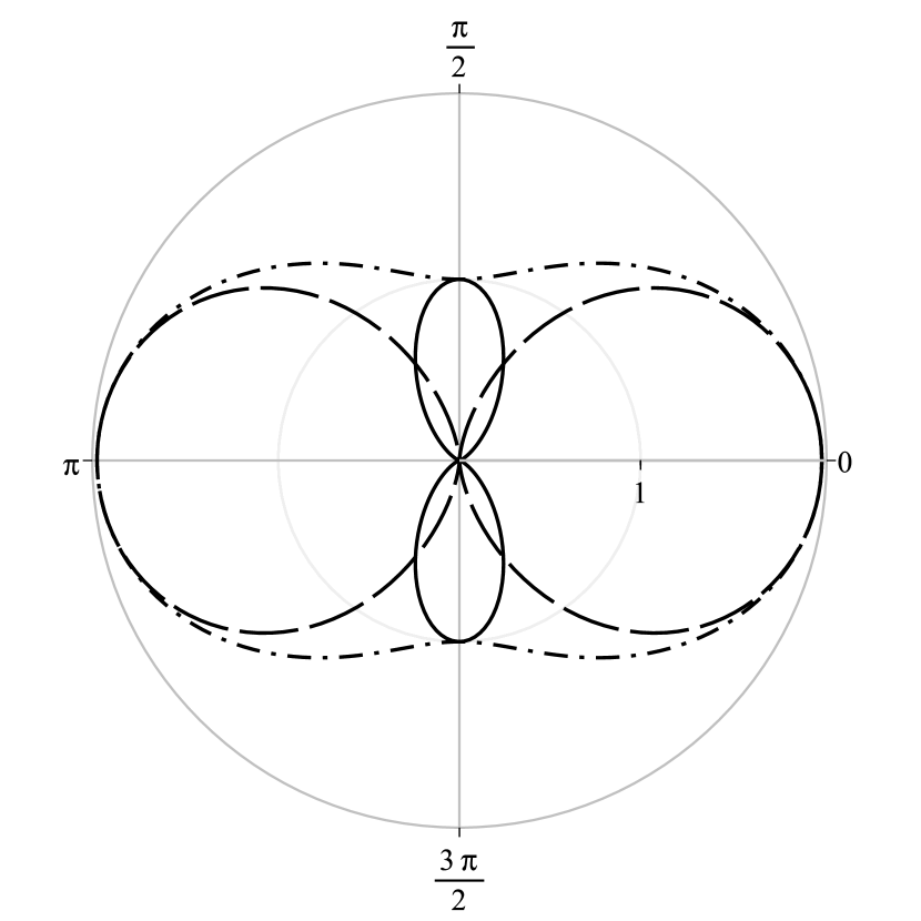
1.a)

1.b)

Figure 1: Angular distribution of CR polarization components (a) and angular dependence of the linear and circular polarization degrees (b). Arbitrary units are used.

3 Polarization and emissivity of the relativistic dipole radiation

Let’s consider an electron in the magnetic field, with the following values of the velocity components in the laboratory frame

$$\upsilon_{\parallel}\simeq c,\qquad\gamma_{\parallel}=\frac{1}{\sqrt{1-\frac{\upsilon_{\parallel}^{2}}{c^{2}}}}\gg 1,$$

$$\upsilon_{\perp}\ll c\sqrt{1-\frac{\upsilon_{\parallel}^{2}}{c^{2}}}=\frac{c}{\gamma_{\parallel}}.$$ (9)

The trajectory of the electron is helical, with the helix step significantly larger than it’s radius (see Fig. 2).

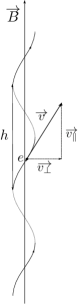
Figure 2: The RDR trajectory: electron moves on helix along the magnetic field; $h$ is the helix step.

The radiation provided by such system is called Zheleznyakov (1997) Relativistic Dipole (RDR). The properties of RDR have been considered in detail in Epstein (1973). The calculations of the angular distributions of RDR emissivity power, and both types of polarization in the laboratory frame, where the electron is moving along the magnetic field to the observer with the velocity $\upsilon_{\parallel}$, may be calculated by making Lorentz transformation in (4),(6),(7). The angle $\vartheta_{0}$ and velocity $\upsilon_{\perp 0}$ in the Larmor circle frame are connected with the angle $\vartheta$ and velocity $\upsilon_{\perp}$ in the laboratory frame as ($\beta_{\parallel}=\upsilon_{\parallel}/c)$

$$\begin{split}\sin\vartheta_{0}=\frac{\sin\vartheta\sqrt{1-\beta_{\parallel}^{2}}}{1-\beta_{\parallel}\cos{\vartheta}},\qquad\cos{\vartheta_{0}}=\frac{{\cos{\vartheta}-\beta_{\parallel}}}{1-\beta_{\parallel}\cos{\vartheta}},\\ \upsilon_{\perp 0}=\gamma_{\parallel}\upsilon_{\perp}.\end{split}$$ (10)

Expressions for the linear and circular polarization degrees in the laboratory frame are obtained from (6),(7), with account of (10), as

$$\rho_{l}=\frac{1-\left(\frac{\cos{\vartheta}-\beta_{\parallel}}{1-\beta_{\parallel}\cos{\vartheta}}\right)^{2}}{1+\left(\frac{\cos{\vartheta}-\beta_{\parallel}}{1-\beta_{\parallel}\cos{\vartheta}}\right)^{2}},\qquad\rho_{c}=\frac{2\frac{\cos{\vartheta}-\beta_{\parallel}}{1-\beta_{\parallel}\cos{\vartheta}}}{1+\left(\frac{\cos{\vartheta}-\beta_{\parallel}}{1-\beta_{\parallel}\cos{\vartheta}}\right)^{2}}.$$ (11)

It follows from (4), (10) that RDR radiation is emitted in a small angle ($\vartheta\lesssim 1/\gamma_{\parallel}$), along the magnetic field direction. We have, by definition, $\beta_{\parallel}^{2}=1-(1/\gamma_{\parallel}^{2})$. For small $\vartheta$, and large $\gamma_{\parallel}$ we have the following expansions

$$\beta_{\parallel}\approx 1-\frac{1}{2\gamma_{\parallel}^{2}}-\frac{1}{8\gamma_{\parallel}^{4}},\quad$$

$$\cos\vartheta\approx 1-\frac{\vartheta^{2}}{2}+\frac{\vartheta^{4}}{24},\quad\cos^{2}\vartheta\approx 1-\vartheta^{2}+\frac{\vartheta^{4}}{3},$$ (12)

It is convenient Bordovitsyn (1999), to introduce a variable

$$\psi=\gamma_{\parallel}\vartheta.$$ (13)

With account of (13) we obtain from (12) the expressions

$$1-\beta_{\parallel}\cos{\vartheta}\approx\frac{1}{2\gamma_{\parallel}^{2}}\left(1+\psi^{2}\right),\qquad\cos{\vartheta}-\beta_{\parallel}\approx\frac{1}{2\gamma_{\parallel}^{2}}\left(1-\psi^{2}\right).$$ (14)

The emission of RDR is monochromatic in the laboratory frame in any given direction, with the frequency and polarization depending on the angle $\theta$. The angular frequency distribution is obtained from the relations for Doppler effect Landau, Lifshitz (1975) (see also Epstein (1973)), which, with account of (14), are written for the time interval $dt$ and the frequency $\omega$, as

$$\quad dt_{0}=dt\sqrt{1-\beta_{\parallel}^{2}},$$ (15)

$$\omega=\omega_{B}\frac{\sqrt{1-\beta_{\parallel}^{2}}}{1-\beta_{\parallel}\cos\vartheta},\quad 2\gamma_{\parallel}\omega_{B}\geq\omega\geq\frac{\omega_{B}}{2\gamma_{\parallel}}\quad{\rm at}\quad 0\leq\vartheta\leq\pi.$$

Approximately we have

$$\omega\approx\frac{2\gamma_{\parallel}\omega_{B}}{1+\psi^{2}},\quad\psi^{2}=\frac{2\gamma_{\parallel}\omega_{B}}{\omega}-1.$$ (16)

Angular dependencies of the polarization degrees in the laboratory frame from (11), with account of (13),(15) are written as Epstein (1973):

$$\rho_{l}(\omega)\approx 2\frac{\psi^{2}}{1+\psi^{4}}=\frac{\omega\left(2\gamma_{\parallel}\omega_{B}-\omega\right)}{\omega^{2}-2\gamma_{\parallel}\omega\omega_{B}+2\gamma_{\parallel}^{2}\omega_{B}^{2}},$$ (17)

$$\rho_{c}(\omega)\approx\frac{1-\psi^{4}}{1+\psi^{4}}=\frac{2\gamma_{\parallel}\omega_{B}\left(\omega-\gamma_{\parallel}\omega_{B}\right)}{\omega^{2}-2\gamma_{\parallel}\omega\omega_{B}+2\gamma_{\parallel}^{2}\omega_{B}^{2}}.$$ (18)

The relative graphics of angular dependencies are presented on Figs 3 – 6.

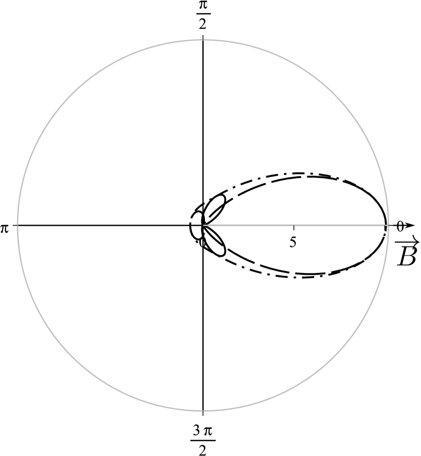
3.1

3.2

Figure 3: Angular distribution of RDR polarization components for different values of Lorentz parameters: 3.1) $\gamma_{\parallel}=1.1$; 3.2) $\gamma_{\parallel}=1.5$. Arbitrary units are used.

4.1

4.2

Figure 4: Angular dependence of the linear and circular polarization degrees for different values of Lorentz parameters: 4.1) $\gamma_{\parallel}=1.1$; 4.2) $\gamma_{\parallel}=1.5$. Arbitrary units are used.

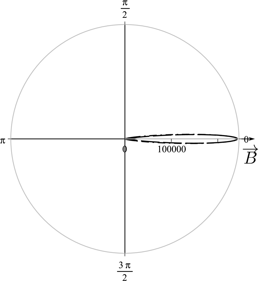
5.1

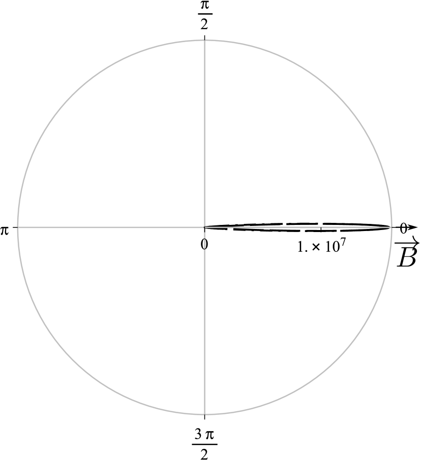
5.2

Figure 5: Angular distribution of RDR polarization components for different values of Lorentz parameters: 5.1) $\gamma_{\parallel}=3.0$; 5.2) $\gamma_{\parallel}=10.0$. Arbitrary units are used.

6.1

6.2

Figure 6: Angular dependence of the linear and circular polarization degrees for different values of Lorentz parameters: 6.1) $\gamma_{\parallel}=3.0$; 6.2) $\gamma_{\parallel}=10.0$. Arbitrary units are used.

The differential power of the radiation in the unity of the solid angle $\Omega$, with $d\Omega=\sin\vartheta d\vartheta d\varphi$, time $t$, and frequency is obtained from (4), with account of (10), (15), and relations

$$d\Omega_{0}=d\Omega\frac{d\cos\vartheta_{0}}{d\cos\vartheta}=d\Omega\frac{1-\beta_{\parallel}^{2}}{(1-\beta_{\parallel}\cos\vartheta)^{2}},$$ (19)

We have than from (4), using (10),(15), the expression for the differential emissivity in the laboratory frame as (see Epstein (1973))

$$\begin{split}W=W_{0}\frac{(1-\beta_{\parallel}^{2})^{3/2}}{(1-\beta_{\parallel}\cos\vartheta)^{2}}=\frac{e^{2}\omega^{2}_{B}\upsilon_{\perp 0}^{2}}{8\pi c^{3}}\left[1+\frac{({\cos{\vartheta}-\beta_{\parallel}})^{2}}{(1-\beta_{\parallel}\cos{\vartheta})^{2}}\right]\\ \times\frac{(1-\beta_{\parallel}^{2})^{3/2}}{(1-\beta_{\parallel}\cos\vartheta)^{2}}\delta[\gamma_{\parallel}\omega(1-\beta_{\parallel}\cos\vartheta)-\omega_{B}].\end{split}$$ (20)

After transformation of $\delta$-function we have

$$W=\frac{e^{2}\omega^{2}_{B}\upsilon_{\perp 0}^{2}}{8\pi c^{3}\gamma_{\parallel}}\left[1+\frac{({\cos{\vartheta}-\beta_{\parallel}})^{2}}{(1-\beta_{\parallel}\cos{\vartheta})^{2}}\right]$$ (21)

$$\times\frac{(1-\beta_{\parallel}^{2})^{3/2}}{(1-\beta_{\parallel}\cos\vartheta)^{3}}\delta\left[\omega-\frac{\omega_{B}}{\gamma_{\parallel}(1-\beta_{\parallel}\cos\vartheta)}\right].$$

Approximately we have

$$W\approx\frac{2e^{2}\omega^{2}_{B}\gamma_{\parallel}^{2}\upsilon_{\perp 0}^{2}}{\pi c^{3}}\frac{1+\psi^{4}}{(1+\psi^{2})^{5}}\delta\left(\omega-\frac{2\gamma_{\parallel}\omega_{B}}{1+\psi^{2}}\right).$$ (22)

Using (16) we obtain in the laboratory frame Epstein (1973))

$$W\approx\frac{e^{2}\upsilon_{\perp 0}^{2}\omega^{3}}{4\pi c^{3}\gamma_{\parallel}\omega_{B}}\left(1-\frac{\omega}{\gamma_{\parallel}\omega_{B}}+\frac{\omega^{2}}{2\gamma_{\parallel}^{2}\omega_{B}^{2}}\right)$$ (23)

$$\times\delta\left(\omega-\frac{2\gamma_{\parallel}\omega_{B}}{1+\psi^{2}}\right){\rm\frac{erg}{s\cdot sterad\cdot Hz}}.$$

The spectral distribution of RDR is obtained after integration over $d\Omega$

$$W(\omega)=\int_{\Omega}W\,d\Omega\,\,{\rm\frac{erg}{s\cdot Hz}},$$ (24)

and the total emissivity

$$W_{tot}=\int_{0}^{\omega_{max}}W(\omega)\,d\omega\,\,{\rm\frac{erg}{s}}.$$ (25)

Taking into account (13),(16), we have the relations for $\delta$-function as

$$2\pi\delta\left(\omega-\frac{2\gamma_{\parallel}\omega_{B}}{1+\psi^{2}}\right)\sin\theta d\theta d\omega\approx\pi\delta\left(\omega-\frac{2\gamma_{\parallel}\omega_{B}}{1+\psi^{2}}\right)d\theta^{2}d\omega$$ (26)

$$=\pi\frac{1+\psi^{2}}{\gamma_{\parallel}^{2}\omega}\delta\left(1+\psi^{2}-\frac{2\gamma_{\parallel}\omega_{B}}{\omega}\right)d(\psi^{2}+1)d\omega,$$

After integration in (24), with account of (26), we obtain

$$W(\omega)=\frac{e^{2}\upsilon_{\perp 0}^{2}\omega^{2}}{4c^{3}\gamma_{\parallel}^{3}\omega_{B}}\left(1-\frac{\omega}{\gamma_{\parallel}\omega_{B}}+\frac{\omega^{2}}{2\gamma_{\parallel}^{2}\omega_{B}^{2}}\right)\times\frac{2\gamma_{\parallel}\omega_{B}}{\omega}$$ (27)

$$=\frac{e^{2}\upsilon_{\perp 0}^{2}\omega}{2c^{3}\gamma_{\parallel}^{2}}\left(1-\frac{\omega}{\gamma_{\parallel}\omega_{B}}+\frac{\omega^{2}}{2\gamma_{\parallel}^{2}\omega_{B}^{2}}\right).$$

The total emissivity, defining the rate of the energy loss of a particle, is obtained after integration of (27), with $\omega_{max}=2\gamma_{\parallel}\omega_{B}$ from (15) as

$$W_{tot}=\int_{0}^{\omega_{max}}W(\omega)\,d\omega=\frac{2e^{2}\upsilon_{\perp 0}^{2}\omega_{B}^{2}}{3c^{3}}\,\,{\rm\frac{erg}{s}},$$ (28)

in accordance with (5).

4 Observational properties of relativistic dipole radiation

We consider here, that the angular size of the aperture of the X-ray detector $\Delta\vartheta_{X}$ is much larger than the characteristic beam width of RDR $\vartheta_{RDR}=1/\gamma_{\parallel}$, so that $\Delta\vartheta_{X}\gg 1/\gamma_{\parallel}$, $\gamma_{\parallel}\gg 1$. If the angular size of the hot spot on the neutron star magnetic poles $\vartheta_{hs}\gg\vartheta_{RDR}$, than the registered X-ray RDR radiation is coming from the part of the hot spot, and is lasted during the time $\tau_{RDR}\approx P\,\vartheta_{hs}/2\pi$. It is decreasing abruptly outside this time interval. Note that in the case of ordinary cyclotron radiation its intensity is decreasing smoothly because of almost isotropic radiation diagram $\sim(1+\cos^{2}{\vartheta_{0}})$, according to (4).

4.1 RDR line widening

Let us mention 3 mechanisms of the line widening in the magneto dipole radiation.

1) A variable magnetic field $B$ in the region of the line formation. This mechanism is working in the cyclotron radiation of nonrelativistic electrons, emitting the line at frequency $\omega=\omega_{B}=\frac{eB}{m_{e}c}$, as well as in RDR where the frequency of radiation in the frame of the Larmor circle is changing similarly.

Two other mechanisms are characteristic only to the RDR.

2) The distribution of electrons over the parallel momentum $p_{\parallel}$ may be presented as Baushev and Bisnovatyi-Kogan (1999)

$$f_{e}(p_{\parallel})=\frac{n_{e}}{\sqrt{\pi\sigma}}\exp\left(-\frac{(p_{\parallel}-a)^{2}}{\sigma^{2}}\right).$$ (29)

Such distribution of electrons leads to widening of the line as Baushev and Bisnovatyi-Kogan (1999)

$$\Delta\omega=\omega_{B}\frac{2\sigma}{m_{e}c}.$$ (30)

For narrow momentum distribution of electrons $\sigma\ll a$ we have

$$\Delta\omega\ll\omega_{B}\frac{2a}{m_{e}c}\approx 2\omega_{B}\gamma_{\parallel}.$$ (31)

In this case the line width may be very narrow. If $\sigma<\frac{m_{e}c}{2}$, the width of the line will be

$$\frac{\Delta\omega}{\omega}<\frac{1}{\gamma_{\parallel}}.$$ (32)

3) In the case of large $\gamma_{\parallel}\gg 1$ the width of the beam is much smaller than the telescope aperture, and the RDR radiation coming from all the beam is registered, with the spectrum (27). Denoting $x=\frac{\omega}{\gamma_{\parallel}\omega_{B}}$, the frequency distribution in the registered signal (27) may be written as

$$W(\omega)\sim\tilde{W}(x)=x(1-x+\frac{x^{2}}{2}),\quad\frac{1}{2\gamma_{\parallel}^{2}}<x<2.$$ (33)

Here $\tilde{W}_{max}=2$ at $x_{max}=2$, the median emissivity $W=1$ is reached at $x_{med}\approx 1.52$, the 50% and 90% of emission is concentrated inside $1.53<x<2$, and $0.63<x<2$ respectively, when

$$\frac{W}{W_{tot}}=\frac{\int_{x_{50,90}}^{2}x(1-x+\frac{x^{2}}{2})dx}{\int_{0}^{2}x(1-x+\frac{x^{2}}{2})dx}=0.5,\,\,0.9$$ (34)

respectively. The observed average frequency of the RDR therefore, corresponds to $x\approx 1.5$. The effective width of the line is about $\delta\omega\approx 0.25\omega_{max}$. The form of the line on the photon counts figure $n_{\gamma}(\omega)$ follows the law

$$n_{\gamma}(x)=1-x+\frac{x^{2}}{2},\quad{\rm at}\quad\frac{1}{2\gamma_{\parallel}^{2}}<x<2,$$ (35)

with a smooth slope at lower frequencies and abrupt brake at $x=2$, $\omega=2\gamma_{\parallel}\omega_{B}$. Stress, that this form of the line is present for monoenergetic electron beam with $\gamma_{\parallel}$ equal for all electrons. This type of widening takes place only in the RDR mechanism, and the form of the magneto-dipole line may be used for distinguishing between the cyclotron and RDR mechanisms. Note that in presence of other widening mechanisms the line may become even wider, but should preserve characteristic feature of this mechanism. The form of the line $\tilde{W}(x)$ and the frequency distribution of the photons are shown on Figs 7 and 8.

Figure 7: The frequency distribution of energy in the RDR line.

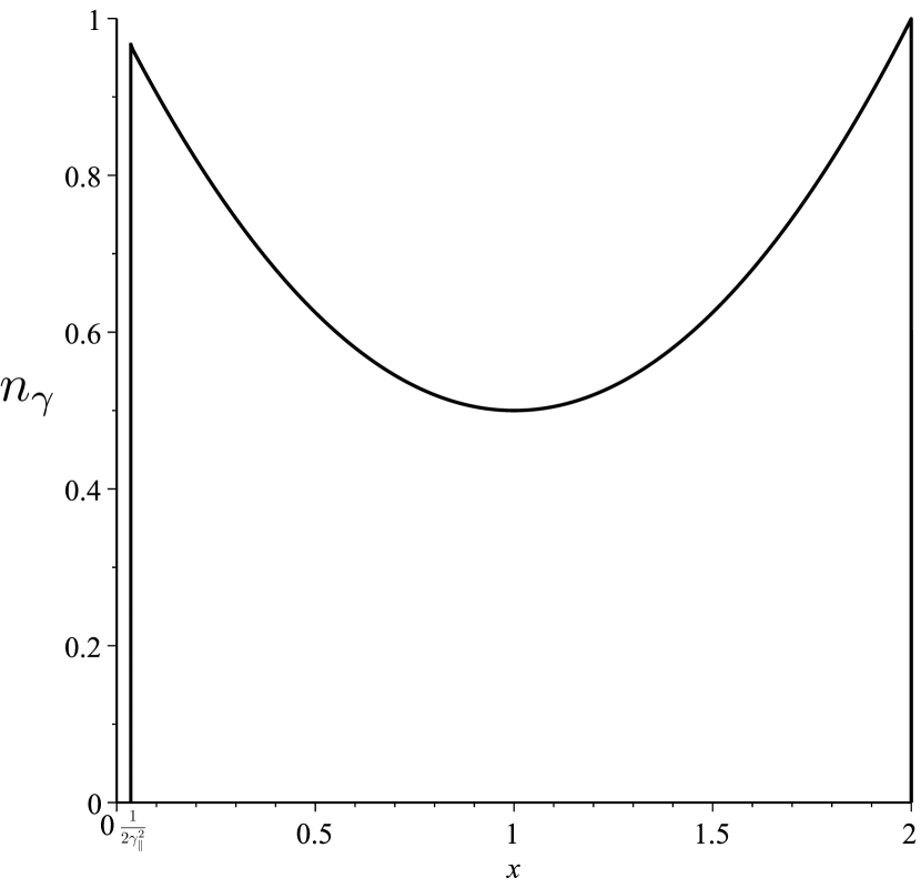
Figure 8: The frequency distribution of the photons. The symmetrical form of the profile corresponds to the symmetry of the angular distribution of the radiation (see Fig. 1).

4.2 Polarization properties

Linear $W_{l}(\omega)$ and circular $W_{c}(\omega)$ parts of the total radiation, using (17), (18), (27), may be expressed in the following way

$$W_{l}(\omega)=W(\omega)\rho_{l}^{2}(\omega)=\frac{e^{2}v_{\perp 0}^{2}\omega_{B}}{2c^{3}\gamma_{\parallel}^{2}}x^{3}\frac{(1-\frac{x}{2})^{2}}{1-x+\frac{x^{2}}{2}},$$ (36)

$$W_{c}(\omega)=W(\omega)\rho_{l}^{2}(\omega)=\frac{e^{2}v_{\perp 0}^{2}\omega_{B}}{2c^{3}\gamma_{\parallel}^{2}}x\frac{(1-x)^{2}}{1-x+\frac{x^{2}}{2}}.$$ (37)

Here $x=\frac{\omega}{\gamma_{\parallel}\omega_{B}}$, $0<x<2$. It is easy to show that $W_{l}(\omega)+W_{c}(\omega)=W(\omega)$ from (27). The linear polarization of the total radiation in the beam $W_{l}$ is obtained by integration over the frequency, it gives

$$W_{l}=\int_{0}^{2}W_{l}(\omega)dx=\frac{e^{2}v_{\perp 0}^{2}\omega_{B}}{2c^{3}\gamma_{\parallel}^{2}}\int_{0}^{2}x^{3}\frac{(1-\frac{x}{2})^{2}}{1-x+\frac{x^{2}}{2}}dx=$$ (38)

$$=(\pi-\frac{8}{3})\frac{e^{2}v_{\perp 0}^{2}\omega_{B}}{2c^{3}\gamma_{\parallel}^{2}}.$$

The linearly polarized part of the radiation in the beam $RDR_{l}$ is defined as

$$RDR_{l}=\frac{W_{l}}{W_{tot}}=\frac{3}{4}\int_{0}^{2}x^{3}\frac{(1-\frac{x}{2})^{2}}{1-x+\frac{x^{2}}{2}}dx=\frac{3}{4}(\pi-\frac{8}{3})\approx$$ (39)

$$\approx\frac{3}{4}\cdot 0.475\approx 0.356.$$

The circularly polarized part of the beam radiation has different sign in the wavelength intervals $\frac{\omega_{B}}{2\gamma_{\parallel}}<\omega<\gamma_{\parallel}\omega_{B}$ ($0<x<1$), and $\omega_{B}\gamma_{\parallel}<\omega<2\gamma_{\parallel}\omega_{B}$ ($1<x<2$). The circularly polarized part of the radiation at lower frequencies $RDR_{c1}$ ($0<x<1$) is determined as

$$RDR_{cl}=\frac{W_{c1}}{W_{tot1}}$$

$$=\left[\int_{0}^{1}x\frac{(1-x)^{2}}{1-x+\frac{x^{2}}{2}}dx\right]/\left[\int_{0}^{1}x(1-x+\frac{x^{2}}{2})\right]$$

$$=(\ln 2-\frac{\pi}{2}+1)/\frac{7}{24}=\frac{0.122}{0.292}\approx 0.418.$$ (40)

The circularly polarized part of the radiation at higher frequencies $RDR_{c2}$ ($1<x<2$) has an opposite sign of polarization, and is determined as

$$RDR_{c2}=\frac{W_{c2}}{W_{tot2}}$$

$$=\left[\int_{1}^{2}x\frac{(1-x)^{2}}{1-x+\frac{x^{2}}{2}}dx\right]/\left[\int_{1}^{2}x(1-x+\frac{x^{2}}{2})\right]$$

$$=(3-\ln 2-\frac{\pi}{2})/\frac{25}{24}=\frac{0.736}{1.042}\approx 0.707.$$ (41)

5 Discussion

The analysis of two model of the magneto dipole mechanism of the line formation had shown important features, by measuring of which the cyclotron model may be distinguished from the RDR model with strongly anisotropic electron distribution. The angular distribution in these models is very different, quasi-isotropic in the cyclotron model, and strongly anisotropic in RDR. Nevertheless, in observing these, usually rather weak lines, it is hardly possible to obtain a definite answer about the angular distribution, due to many contaminating factors. Different form of the line, and different observed light curves, predicted by theory for these lines could help more, when measured, but for weak lines it seems also very difficult. The most distinct difference between the cyclotron and RDR mechanisms of the line formation may be seen in their polarization features. The measurements of the hard X-ray polarization are discussed for more than 40 years, but still there is no space mission for these measurements. The linear X-ray polarization which is measured should be close to zero for the cyclotron radiation from the hot magnetic pole, while the radiation produced in RDR model should have about 35% of the linear polarization in the line, what is sufficiently well distinguished difference, which could be taken into account in the construction of the hard X-ray polarimeter. The first source with the detected magnetic dipole line Her X-1 is still the best target for this investigation.

The line emitted by non-relativistic electrons in the magnetic field has the same cyclotron frequency. Its harmonics are highly suppressed at $kT\ll m_{e}c^{2}$, what is expected in the accretion disk and in the accretion column. The observed line width originating from photons of the relativistic dipole radiation coming from different angles is forming one broad line, contrary to separate harmonics in the cyclotron model. The second harmonic in the case of relativistic dipole radiation should form another line of almost the same width at double energy. There is still not clear wether the second "cyclotron" harmonics is present in the X-ray spectrum of Her X1 (Trümper at al., 1978; Enoto et al., 2008; Fürst et al., 2013).

The influence of the line broadening due to the distribution over the parallel electron momentum is considered by Baushev and Bisnovatyi-Kogan (1999). According to (32), the broadening is small when the scattering momentum is non-relativistic. With increasing of $\sigma$ over $m_{e}c$, the broadening increases, and the resulting line broadening is the combination of the angular and scattering action. Nevertheless, it is very important that for any scattering in a parallel direction the parameters of the polarization do not change for any large $\gamma_{\parallel}$, which are considered in this model, and the criteria for the choice between models remains valid.

References

- AstroH (2015) AstroH (2015) Astronomical project Astro-H: http://astro-h.isas.jaxa.jp
- Baushev and Bisnovatyi-Kogan (1999) Baushev A.N., Bisnovatyi-Kogan G.S. (1999) Astronomical Reports, 43, 241
- Bisnovatyi-Kogan (1973) Bisnovatyi-Kogan G.S. (1973) AZh, 50, 902
- Bisnovatyi-Kogan and Fridman (1969) Bisnovatyi-Kogan G.S., Fridman A.M. (1969) AZh, 46, 721
- Bisnovatyi-Kogan and Komberg (1974) Bisnovatyi-Kogan G.S., Komberg B.V. (1974) AZh, 51, 373
- Bordovitsyn (1999) Bordovitsyn V.A. ed. (1999) Synchrotron radiation theory and its development, Singapour, World Scientific
- Deeter, et al. (1998) Deeter J.E., Scott D.M., Boynton P.E., Miyamoto S., Kitamoto S., Takahama S., Nagase F. (1998) ApJ, 502, 802
- Enoto, et al. (2008) Enoto T., Makishima K., Terada Y., Mihara T., Nakazawa K., Ueda T., Dotani T., Kokubun M., Nagase F., Naik S., Suzuki M., Nakajima M., and Takahashi M. (2008) Publ. Astron. Soc. Japan 60, S57
- Epstein (1973) Epstein R. (1973) ApJ, 183, 593
- Fürst (2013) Fürst F., Grefenstette W.B., Staubert R., Tomsick J.A., Bachetti M., Barret D., Bellm E.C., Boggs S.E., Chenevez J., Christensen F.E., Craig W.W., Hailey C.J., Harrison F., Klochkov D., Madsen K.K., Pottschmidt K., Stern D., Walton D.J., Wilms J., and Zhang W. (2013) ApJ, 779, 69
- Gruber, et al. (1980) Gruber D.E., Matteson J.L., Nolan P.L., Knight F.K., Baity W.A., Rothschild R.E., Peterson L.E., Hoffman J.A., Scheepmaker A., Wheaton W.A., Primini F.A., Levine A.M., Lewin W.H.G. (1980) ApJ.(Letters), 240, L27
- Kislat, et al. (2015) Kislat F., Beilicke M., Guo Q., Zajczyk A., Krawczynski H. (2015) Astropart. Phys. 64, 40
- Landau, Lifshitz (1975) Landau L.D., Lifshitz E.M. (1975) The classical theory of fields, Oxford: Pergamon Press
- Lorimer (2005) Lorimer D.R. (2005) Living Reviews in Relativity 8: 7-82; http://www.livingreviews.org/lrr-2005-7
- Pearce, et al. (2012) Pearce M. Florén H.-G., Jackson M., Kamae T., Kiss M., Kole M., Moretti E., Olofsson G., Rydström S., Strömberg J.-E., Takahashi H. (2012) arXiv:1211.5094v2
- Postnov, et al. (2012) Postnov K., Shakura N., Staubert R., Kochetkova A., Klochkov D., Wilms J. (2013) MNRAS, 435, 1147
- Staubert, et al. (2012) Staubert R., Klochkov D., Vasco D., Postnov K., Shakura N., Wilms J., and Rothschild R.E. (2013) A&A 550, A110
- Scott, et al. (2000) Scott D.M., Leahy D.A., Wilson R.B. (2000) ApJ, 539, 392
- Sheffer, et al. (1992) Sheffer E.K., Kopaeva I.F., Averintsev M.B., Bisnovatyi-Kogan G.S., Golynskaya I.M., Gurin L.S., Dyachkov A.V., Zenchenko V.M., Kurt V.G., Mizyakina T.A., Mironova E.N., Sklyankin V.A., Smirnov A.S., Titarchuk L.G., Shamolin V.M., Shafer,] E.Y., Shmelkin A.A., Giovannelli F. (1992) AZh, 1992, 69, 82
- Trubnikov (1961) Trubnikov V.A. (1961) Phys. Fluids, 4, 195
- Trümper (1978) Trümper J., Pietsch W., Reppin C., Voges W., Staubert R., Kendziorra E. (1978) ApJ lett. 219, L105
- Tuelle, et al. (1984) Tueller J., Cline T.L., Teegarden B.J., Paciesas W.S., Boclet D., Durouchoux Ph., Hameury J.M., Prantzos N., Haymes R.C. (1984) ApJ, 279, 177
- Ubertini, et al. (1980) Ubertini P., Bazzano, A., La Padula C., Polcaro V.F., Manchanda R.K. (1980) Proc. 17th Int. Cosmic-Ray Conf., Paris, 1, 99
- Voges, et al. (1982) Voges W., Pietsch W., Reppin C., Trümper J., Kendziorra E., Staubert R. (1982) ApJ, 263, 803
- Zheleznyakov (1997) Zheleznyakov V.V. 1997, Radiation in the astrophysical plasma, Moscow. Yanus-K.(in Russian)