Near-optimal small-depth lower bounds
for small distance connectivity

Abstract

We show that any depth-$d$ circuit for determining whether an $n$-node graph has an $s$-to-$t$ path of length at most $k$ must have size $n^{\Omega(k^{1/d}/d)}$. The previous best circuit size lower bounds for this problem were $n^{k^{\exp(-O(d))}}$ (due to Beame, Impagliazzo, and Pitassi [BIP98]) and $n^{\Omega((\log k)/d)}$ (following from a recent formula size lower bound of Rossman [Ros14]). Our lower bound is quite close to optimal, since a simple construction gives depth-$d$ circuits of size $n^{O(k^{2/d})}$ for this problem (and strengthening our bound even to $n^{k^{\Omega(1/d)}}$ would require proving that undirected connectivity is not in $\mathsf{NC^{1}}.$)

Our proof is by reduction to a new lower bound on the size of small-depth circuits computing a skewed variant of the “Sipser functions” that have played an important role in classical circuit lower bounds [Sip83, Yao85, Hås86]. A key ingredient in our proof of the required lower bound for these Sipser-like functions is the use of random projections, an extension of random restrictions which were recently employed in [RST15]. Random projections allow us to obtain sharper quantitative bounds while employing simpler arguments, both conceptually and technically, than in the previous works [Ajt89, BPU92, BIP98, Ros14].

1 Introduction

Graph connectivity problems are of great interest in theoretical computer science, both from an algorithmic and a computational complexity perspective. The “$st$-connectivity,” or $\mathit{STCONN}$, problem — given an $n$-node graph $G$ with two distinguished vertices $s$ and $t$, is there a path of edges from $s$ to $t$? — plays a particularly central role. One longstanding question is whether any improvement is possible on Savitch’s $O((\log n)^{2})$-space algorithm [Sav70], based on “repeated squaring,” for the directed $\mathit{STCONN}$ problem; since this problem is complete for $\mathsf{NL}$, any such improvement would show that $\mathsf{NL}\subseteq\mathsf{SPACE}(o(\log^{2}n))$, and hence would have a profound impact on our understanding of non-deterministic space complexity. Wigderson’s survey [Wig92] provides a now somewhat old, but still very useful, overview of early results on connectivity problems.

In this paper we consider the “small distance connectivity” problem $\mathit{STCONN}(k(n))$ which is defined as follows. The input is the adjacency matrix of an undirected $n$-vertex graph $G$ which has two distinguished vertices $s$ and $t$, and the problem is to determine whether $G$ contains a path of length at most $k(n)$ from $s$ to $t$. We study this problem from the perspective of small-depth circuit complexity; for a given depth $d$ (which may depend on $k$), we are interested in the size of unbounded fan-in depth-$d$ circuits of $\mathrm{AND}$, $\mathrm{OR}$, and $\mathrm{NOT}$ gates that compute $\mathit{STCONN}(k(n))$. (As several authors [BIP98, Ros14] have observed, the directed and undirected versions of the $\mathit{STCONN}(k(n))$ problems are essentially equivalent via a simple reduction that converts a directed graph into a layered undirected graph; for simplicity we focus on the undirected problem in this paper.)

An impetus for this study comes from the above-mentioned question about Savitch’s algorithm. As noted by Wigderson [Wig92], a simple reduction shows that if Savitch’s algorithm is optimal, then for all $k$ polynomial-size unbounded fan-in circuits for $\mathit{STCONN}(k(n))$ must have depth $\Omega(\log k)$. By giving lower bounds on the size of small-depth circuits for $\mathit{STCONN}(k(n))$, Beame, Impagliazzo, and Pitassi [BIP98] have shown that depth $\Omega(\log\log k)$ is required for $k(n)\leq\log n$, and more recently Rossman [Ros14] has shown that depth $\Omega(\log k)$ is required for $k(n)\leq\log\log n$. These bounds for restricted ranges of $k$ motivate further study of the circuit complexity of small-depth circuits for $\mathit{STCONN}(k(n)).$ Below we give a more thorough discussion of both upper and lower bounds for this problem, before presenting our new results.

1.1 Prior results

Upper bounds (folklore). A natural approach to obtain efficient circuits for $\mathit{STCONN}(k(n))$ is by repeated squaring of the input adjacency matrix. If $x_{i,j}$ is the input variable that takes value 1 if edge $\{i,j\}$ is present in the input graph, then the graph contains a path of length at most 2 from $i$ to $j$ if and only if the depth-2 circuit $\bigvee_{k=1}^{n}(x_{i,k}\wedge x_{k,j})$ is satisfied (assuming that $x_{i,i}=1$ for every $i$). Iterating this construction yields a circuit of size $\mathrm{poly}(n)$ and depth $2\log k$ that computes $\mathit{STCONN}(k(n))$, whenever $k$ is a power of two.

For smaller depths, a natural extension of this approach leads to the following construction. Let $G_{0}$ be the input graph. For every pair of nodes $u,v$ in $G_{0}$, check by exhaustive search for paths of length at most $t=k^{1/d}$ connecting these nodes. (We assume that $k^{1/d}$ is an integer in order to avoid unnecessary technical details.) Note that this can be done simultaneously for every pair of nodes by a (multi-output) depth-2 $\mathrm{OR}$-of-$\mathrm{AND}$s circuit of size $n^{t+O(1)}$. Let $G_{1}$ be a new graph that has an edge between $u$ and $v$ if and only if a path of length at most $t$ connects these nodes. In general, if we start with $G_{0}$ and repeat this procedure $d$ times, we obtain a sequence of graphs $G_{0},G_{1},\ldots,G_{d}$ for which the following holds: $G_{i}$ has an edge between nodes $u$ and $v$ if and only if they are connected by a path of length at most $t^{i}$ in the initial graph $G_{0}$. In particular, this construction provides a circuit of depth $2d$ and size $n^{k^{1/d}+O(1)}$ that computes $\mathit{STCONN}(k(n))$.

Summarizing this discussion, it follows that for all $k\leq n$ and $\smash{d\leq\log k}$, $\mathit{STCONN}(k(n))$ can be computed by depth-$2d$ circuits of size $\smash{n^{O(k^{1/d})}}$, or equivalently by depth-$d$ circuits of size $\smash{n^{O(k^{2/d})}.}$

Lower bounds. Furst, Saxe, and Sipser [FSS84] were the first to show that $\mathit{STCONN}\stackrel{{\scriptstyle\rm def}}{{=}}\mathit{STCONN}(n)\notin\mathsf{AC^{0}}$ via a reduction from their lower bound against small-depth circuits computing the parity function. By the same reduction, Håstad’s subsequent optimal lower bound against parity [Hås86] implies that depth-$d$ circuits computing $\mathit{STCONN}(k(n))$ must have size $2^{\Omega(k^{1/(d+1)})}$; in particular, for $k(n)=(\log n)^{\omega(1)}$ polynomial-size circuits computing $\mathit{STCONN}(k(n))$ must have depth $d=\Omega(\log k/\log\log n)$. Note, however, that this is not a useful bound for small distance connectivity, since when $k(n)=o(\log n)$ the $\smash{2^{\Omega(k^{1/(d+1)})}}$ lower bound is less than $n$ and hence trivial.

Ajtai [Ajt89] was the first to show that $\mathit{STCONN}(k(n))\notin\mathsf{AC^{0}}$ for all $k(n)=\omega_{n}(1)$; however, his proof did not yield an explicit circuit size lower bound. His approach was further analyzed and simplified by Bellantoni, Pitassi, and Urquhart [BPU92], who showed that this technique gives a (barely super-polynomial) $n^{\Omega(\log^{(d+3)}k)}$ lower bound on the size of depth-$d$ circuits for $\mathit{STCONN}(k(n))$, where $\log^{(i)}$ denotes the $i$-times iterated logarithm. This implies that polynomial-size circuits computing $\mathit{STCONN}(k(n))$ must have depth $\Omega(\log^{*}k)$.

Beame, Impagliazzo, and Pitassi [BIP98] gave a significant quantitative strengthening of Ajtai’s result in the regime where $k(n)$ is not too large. For $k(n)\leq\log n$, they showed that any depth-$d$ circuit for $\mathit{STCONN}(k(n))$ must have size $n^{\Omega(k^{\phi^{-2d}/3})},$ where $\phi=(\sqrt{5}+1)/2$ is the golden ratio. Their arguments are based on a special-purpose “connectivity switching lemma” that they develop, which combines elements of both the Ajtai [Ajt83] “independent set style” switching lemma and the later approach to switching lemmas given by Yao [Yao85], Hastad [Hås86] and Cai [Cai86].

Observe that the [BIP98] lower bound shows that polynomial-size circuits for $\mathit{STCONN}(k(n))$ require depth $\Omega(\log\log k)$ (and as noted above, the [BIP98] lower bound only holds for $k(n)\leq\log n$). Beame et al. asked whether this $\Omega(\log\log k)$ could be improved to $\Omega(\log k)$, which is optimal by the upper bound sketched above. This was achieved recently by Rossman [Ros14], who showed that for $k(n)\leq\log\log n$, polynomial-size circuits for $\mathit{STCONN}(k(n))$ require depth $\Omega(\log k)$. In more detail, he showed that for $k(n)\leq\log\log n$ and $d(n)\leq\log n/(\log\log n)^{O(1)}$, depth-$d$ formulas for $\mathit{STCONN}(k(n))$ require size $n^{\Omega(\log k)}$. By the trivial relation between formulas and circuits (every circuit of size $S$ and depth $d$ is computed by a formula of size $S^{d}$ and depth $d$), this implies that for such $k(n)$ and $d(n)$, depth-$d$ circuits for $\mathit{STCONN}(k(n))$ require size $n^{\Omega((\log k)/d)}.$ While this answers the question of Beame et al., the $n^{\Omega((\log k)/d)}$ circuit size bound that follows from Rossman’s formula size bound is significantly smaller than the $n^{\Omega(k^{\phi^{-2d}/3})}$ circuit size bound of [BIP98] when $d$ is small. Furthermore, Rossman’s result only holds for $k(n)\leq\log\log n$ whereas [BIP98]’s holds for $k(n)\leq\log n$ (and ideally we would like a lower bound for all distances $k(n)\leq n$).

1.2 Our results

	Circuit size	Depth of poly-size circuits	Range of $k$’s
Implicit in [Hås86]	$2^{\Omega(k^{1/(d+1)})}$	$\Omega(\log k/\log\log n)$	All $k$
[Ajt89, BPU92]	$n^{\Omega(\log^{(d+3)}k)}$	$\Omega(\log^{*}k)$	All $k$
[BIP98]	$n^{\Omega(k^{\phi^{-2d}/3})}$	$\Omega(\log\log k)$	$k\leq\log n$
[Ros14]	$n^{\Omega((\log k)/d)}$	$\Omega(\log k)$	$k\leq\log\log n$
Folklore upper bound	$n^{O(k^{2/d})}$	$2\log k$	All $k$
This work	$n^{\Omega(k^{1/d}/d)}$	$\Omega(\log k/\log\log k)$	$k\leq n^{1/5}$
	$n^{\Omega(k^{1/5d}/d)}$		All $k$

Table 1: Previous work and our results on the size of depth-$d$ circuits for $\mathit{STCONN}(k(n))$. The column “Range of $k$’s” indicates the values of $k$ for which the lower bound is proved to hold.

Our main result is a near-optimal lower bound for the small-depth circuit size of $\mathit{STCONN}(k(n))$ for all distances $k(n)\leq n$. We prove the following:

Theorem 1.

For any $k(n)\leq n^{1/5}$ and any $d=d(n)$, any depth-$d$ circuit computing $\mathit{STCONN}(k(n))$ must have size $n^{\Omega(k^{1/d}/d)}$. Furthermore, for any $k(n)\leq n$ and any $d=d(n)$, any depth-$d$ circuit computing $\mathit{STCONN}(k(n))$ must have size $n^{\Omega(k^{1/5d}/d)}$.

Our lower bound is very close to the best possible, given the $n^{O(k^{2/d})}$ upper bound. Indeed, strengthening our theorem to $n^{k^{\Omega(1/d)}}$ for all values of $k$ and $d$ would imply a breakthrough in circuit complexity, showing that unbounded fan-in circuits of depth $o(\log n)$ computing $\mathit{STCONN}$ must have super-polynomial size. Since every function in $\mathsf{NC^{1}}$ can be computed by unbounded fan-in circuits of polynomial size and depth $O(\log n/\log\log n)$ (see e.g. [KPPY84]), such a strengthening would yield an unconditional proof that $\mathit{STCONN}\notin\mathsf{NC^{1}}$.

Comparing to previous work, our $n^{\Omega(k^{1/d}/d)}$ lower bound subsumes the main $n^{\Omega(k^{\phi^{-2d}/3})}$ lower bound result of Beame et al. [BIP98] for all depths $d$, and improves the $n^{\Omega((\log k)/d)}$ circuit size lower bound that follows from Rossman’s formula size lower bound [Ros14] except when $d$ is quite close to $\log k$ (specifically, except when $\Omega(\log k/\log\log k)\leq d\leq O(\log k)$). For large distances $k(n)$ for which the results of [BIP98, Ros14] do not apply (i.e. $k(n)=\omega(\log n)$), our lower bound subsumes the $2^{\Omega(k^{1/(d+1)})}$ lower bound that is implied by [Hås86] for all distances $k(n)\leq n^{1/5}$ and depths $d$, and it subsumes the subsequent $n^{\Omega(\log^{(d+3)}k)}$ lower bound of [Ajt89, BPU92] for all distances $k$ and depths $d$.

Another perspective on Theorem 1 is that it implies that polynomial-size circuits require depth $\Omega(\log k/\log\log k)$ to compute $\mathit{STCONN}(k(n))$ for all distances $k(n)\leq n$. While Rossman’s results give $\Omega(\log k)$, they hold only for the significantly restricted range $k(n)\leq\log\log n$. (And indeed, as noted above a lower bound of $\Omega(\log k)$ for all $k(n)$ would imply that $\mathit{STCONN}\notin\mathsf{NC^{1}}$.)

1.3 Our approach

Previous state-of-the-art results on this problem employed rather sophisticated arguments and involved machinery. Beame et al. [BIP98] (as well as the earlier works of [Ajt89, BPU92]) obtained their lower bounds by considering the $\mathit{STCONN}(k(n))$ problem on layered graphs of permutations, i.e., graphs with $k+1$ layers of $n$ vertices per layer in which the induced graph between adjacent layers is a perfect bipartite matching. They developed a special-purpose “connectivity switching lemma” that bounds the depth of specialized decision trees for randomly-restricted layered graphs. Rossman [Ros14] considered random subgraphs of the “complete $k$-layered graph” (with $k+1$ layers of $n$ vertices and $kn^{2}$ edges) where each edge is independently present with probability $1/n$. At the heart of his proof is an intricate notion of “pathset complexity,” which roughly speaking measures the minimum cost of constructing a set of paths via the operations of union and relational join, subject to certain “density constraints.”

In contrast, we feel that our approach is both conceptually and technically simple. Instead of working with layered permutation graphs or random subgraphs of the complete layered graph, we consider a class of series-parallel graphs that are obtained in a straightforward way (see Section 3) from a skewed variant of the “Sipser functions” that have played an important role in the classical circuit lower bounds of Sipser [Sip83], Yao [Yao85], and Håstad [Hås86]. Briefly, for every $d\in\mathbbm{N}$, the $d$-th Sipser function $\mathsf{Sipser}_{d}$ is a read-once monotone formula with $d$ alternating layers of $\mathrm{AND}$ and $\mathrm{OR}$ gates of fan-in $w$, where $w\in\mathbbm{N}$ is an asymptotic parameter that tends to $\infty$ (and so $\mathsf{Sipser}_{d}$ computes an $n=w^{d}$ variable function). Building on the work of Sipser and Yao, Håstad used the Sipser functions to prove an optimal depth-hierarchy theorem for circuits, showing that for every $d\in\mathbbm{N}$, any depth-$d$ circuit computing $\mathsf{Sipser}_{d+1}$ must have size $\exp(n^{\Omega(1/d)})$.

The skewed variant of the Sipser functions that we use to prove our near-optimal lower bounds for $\mathit{STCONN}(k(n))$ is as follows. For every $d\in\mathbbm{N}$ and $2\leq u\leq w$, the $d$-th $u$-skewed Sipser function, denoted $\mathsf{SkewedSipser}_{u,d}$, is essentially $\mathsf{Sipser}_{2d+1}$ but with the $\mathrm{AND}$ gates having fan-in $u$ rather than $w$ (see Section 3 for a precise definition; as we will see, the number of levels of $\mathrm{AND}$ gates is the key parameter for $\mathsf{SkewedSipser}$, which is why we write $\mathsf{SkewedSipser}_{u,d}$ to denote the $n$-variable formula that has $d$ levels of $\mathrm{AND}$ gates and $d+1$ levels of $\mathrm{OR}$ gates.) Via a simple reduction given in Section 3, we show that to get lower bounds for depth-$d$ circuits computing $\mathit{STCONN}(u^{d})$ on $n$-node graphs, it suffices to prove that depth-$d$ circuits for $\mathsf{SkewedSipser}_{u,d}$ must have large size. Under this reduction the fan-in of the $\mathrm{AND}$ gates is directly related to the length of (potential) paths between $s$ and $t$. This is why we must use a skewed variant of the Sipser function in order to obtain lower bounds for small distance connectivity. We remark that even the case $u=2$ is interesting and can be used to get the $n^{\Omega(k^{1/d}/d)}$ lower bound of Theorem 1 for $k$ up to roughly $2^{\sqrt{\log n}}$. Allowing a range of values for $u$ enables us to get the lower bound for $k$ up to $n^{1/5}$ (as stated in Theorem 1).

Our main technical result of the paper is a lower bound for $\mathsf{SkewedSipser}_{u,d}$, a formula of depth $2d+1$ over $n=n(u,w,d)=u^{d}w^{d+33/100}$ variables (for technical reasons we use a smaller fan-in for the first layer of OR gates next to the inputs).

Theorem 2.

Let $d(w)\geq 1$ and $2\leq u(w)\leq w^{33/100}$, where $w\to\infty$. Then any depth-$d$ circuit computing $\mathsf{SkewedSipser}_{u,d}$ has size at least $w^{\Omega(u)}=n^{\Omega(u/d)}$.

Observe that setting $u=k^{1/d}$ this size lower bound is $n^{\Omega(k^{1/d}/d)}$, and therefore we indeed obtain the lower bound for $\mathit{STCONN}(k(n))$ stated in Theorem 1 as a corollary. As we point out in Section 6 (Remark 18), the lower bound given in Theorem 2 for $\mathsf{SkewedSipser}$ is essentially optimal.

Though they are superficially similar, Theorem 2 and Håstad’s depth hierarchy theorem differ in two important respects. Both result from our goal of using Theorem 2 to get lower bounds for small distance connectivity, and both pose significant challenges in extending Håstad’s proof:

1. Håstad showed that depth-$d$ unbounded fan-in circuits require large size to compute a single highly symmetric “hard function,” namely $\mathsf{Sipser}_{d+1}$. In contrast, toward our goal of understanding the depth-$d$ circuit size of $\mathit{STCONN}(k(n))$ for all values of $k=k(n)$ and $d=d(n)$, we seek lower bounds on the size of depth-$d$ unbounded fan-in circuits computing any one of a spectrum of asymmetric hard functions, namely $\mathsf{SkewedSipser}_{u,d}$ for all $u:=k^{1/d}$ (with stronger quantitative bounds as $k$ and $u$ get larger).

2. To get the strongest possible result in his depth hierarchy theorem, Håstad (like Yao and Sipser) was primarily focused on lower bounding the size of circuits of depth exactly one less than $\mathsf{Sipser}_{d+1}$. In contrast, since in our framework our goal is to lower bound the size of depth-$d$ circuits computing $\mathsf{SkewedSipser}_{u,d}$ (corresponding to $\mathit{STCONN}(k(n))$ with $k=u^{d}$) which has depth $2d+1$, we are interested in the size of circuits of depth (roughly) half that of our hard function $\mathsf{SkewedSipser}_{u,d}$.

In Section 2 we recall the high-level structure of Håstad’s proof of his depth hierarchy theorem (based on the method of random restrictions), highlight the issues that arise due to each of the two differences above, and describe how our techniques — specifically, the method of random projections — allow us to prove Theorem 2 in a clean and simple manner.

2 Håstad’s depth hierarchy theorem, random projections, and proof outline of Theorem 2

Håstad’s depth hierarchy theorem and its proof. Recall that Håstad’s depth hierarchy theorem shows that $\mathsf{Sipser}_{d+1}$ cannot be computed by any circuit $C$ of depth $d$ and size $\exp(n^{O(1/d)}).$ The main idea is to design a sequence of random restrictions $\{\mathcal{R}_{\ell}\}_{2\leq\ell\leq d}$ satisfying two competing requirements:

• Circuit $C$ collapses. The randomly restricted circuit $C\upharpoonright{\boldsymbol{\rho}}^{(d)}\cdots{\boldsymbol{\rho}}^{(2)}$, where ${\boldsymbol{\rho}}^{(\ell)}\leftarrow\mathcal{R}_{\ell}$ for $2\leq\ell\leq d$, collapses to a “simple function” with high probability. This is shown via iterative applications of a switching lemma for the $\mathcal{R}_{\ell}$’s, where each application shows that with high probability a random restriction ${\boldsymbol{\rho}}^{(\ell)}$ decreases the depth of the circuit $C\upharpoonright{\boldsymbol{\rho}}^{(d)}\cdots{\boldsymbol{\rho}}^{(\ell+1)}$ by at least one. The upshot is that while $C$ is a size-$S$ depth-$d$ circuit, $C\upharpoonright{\boldsymbol{\rho}}^{(d)}\cdots{\boldsymbol{\rho}}^{(2)}$ collapses to a small-depth decision tree (i.e. a “simple function”) with high probability.

• Hard function $\mathsf{Sipser}_{d+1}$ retains structure. In contrast with the circuit $C$, the hard function $\mathsf{Sipser}_{d+1}$ is “resilient” against the random restrictions ${\boldsymbol{\rho}}^{(\ell)}\leftarrow\mathcal{R}_{\ell}$. In particular, each random restriction ${\boldsymbol{\rho}}^{(\ell)}$ simplifies $\mathsf{Sipser}$ only by one layer, and so $\mathsf{Sipser}_{d+1}\upharpoonright{\boldsymbol{\rho}}^{(d)}\cdots{\boldsymbol{\rho}}^{(\ell)}$ contains $\mathsf{Sipser}_{\ell}$ as a subfunction with high probability. Therefore, with high probability. $\mathsf{Sipser}_{d+1}\upharpoonright{\boldsymbol{\rho}}^{(d)}\cdots{\boldsymbol{\rho}}^{(2)}$ still contains $\mathsf{Sipser}_{2}$ as a subfunction, and hence is a “well-structured function” which cannot be computed by a small-depth decision tree.

We remind the reader that to satisfy these competing demands, the random restrictions $\{\mathcal{R}_{\ell}\}$ devised by Håstad specifically for his depth hierarchy theorem are not the “usual” random restrictions where each coordinate is independently kept alive with probability $p\in(0,1)$, and set to a uniform bit otherwise (it is not hard to see that $\mathsf{Sipser}$ does not retain structure under these random restrictions). Likewise, the switching lemma for the $\mathcal{R}_{\ell}$’s is not the “standard” switching lemma (which Håstad used to obtain his optimal lower bounds against the parity function). Instead, at the heart of Håstad’s proof are new random restrictions $\{\mathcal{R}_{\ell}\}_{2\leq\ell\leq d}$ designed to satisfy both requirements above: the coordinates of $\mathcal{R}_{\ell}$ are carefully correlated so that $\mathsf{Sipser}_{\ell+1}$ retains structure, and Håstad proved a special-purpose switching lemma showing that $C$ collapses under these carefully tailored new random restrictions.

Issues that arise in our setting. At a technical level (related to point (1) described at the end of Section 1), Håstad’s special-purpose switching lemma is not useful for analyzing our $\mathsf{SkewedSipser}_{u,d}$ formulas for most values of $u=k^{1/d}$ of interest, since they have a “fine structure” that is destroyed by his too-powerful random restrictions. His switching lemma establishes that any DNF of width $n^{O(1/d)}$ collapses to a small-depth decision tree with high probability when it is hit by a random restriction ${\boldsymbol{\rho}}^{(\ell)}\leftarrow\mathcal{R}_{\ell}$. Observe that his hard function $\mathsf{Sipser}_{d+1}$ has DNF-width $\Omega(\sqrt{n})$, so his switching lemma does not apply to it (and indeed as discussed above, hitting $\mathsf{Sipser}_{d+1}$ with his random restriction results in a well-structured function that still contains $\mathsf{Sipser}_{d}$ as a subfunction with high probability). In contrast, in our setting the hard function $\mathsf{SkewedSipser}_{u,d}$ has $d$ levels of $\mathrm{AND}$ gates of fan-in $u$, and in particular, can be written as a DNF of width $u^{d}=k$. So for all $k=k(n)$ and $d=d(n)$ such that $k\ll n^{O(1/d)}$ (indeed, this holds for most values of $k$ and $d$ of interest), the relevant hard function $\mathsf{SkewedSipser}_{u,d}$ collapses to a small-depth decision tree after a single application of Håstad’s random restriction.

Next (related to point (2)), recall that the formula computing Håstad’s hard function $\mathsf{Sipser}_{d+1}$ has a highly regular structure where the fan-ins of all gates — both $\mathrm{AND}$’s and $\mathrm{OR}$’s — are the same. As discussed above, Håstad employs a random restriction which (with high probability) “peels off” a single layer of $\mathsf{Sipser}_{d+1}$ and results in a function that contains $\mathsf{Sipser}_{d}$ as a subfunction. Due to their regular structures, $\mathsf{Sipser}_{d}$ is dual to $\mathsf{Sipser}_{d+1}$ (more precisely, the bottom-layer depth-$2$ subcircuits of $\mathsf{Sipser}_{d}$ are dual to those of $\mathsf{Sipser}_{d+1}$), and this allows Håstad to repeat the same procedure $d-1$ times. In contrast, in our setting we are dealing with the highly asymmetric $\mathsf{SkewedSipser}_{u,d}$ formulas where the fan-ins of the $\mathrm{AND}$ gates are much less than those of the $\mathrm{OR}$ gates. Therefore, in order to reduce to a smaller instance of the same problem, our setup requires that we peel off two layers of $\mathsf{SkewedSipser}_{u,d}$ at a time rather than just one as in Håstad’s argument. To put it another way, while Håstad’s switching lemma uses a single layer of his hard function $\mathsf{Sipser}_{d+1}$ (i.e. disjoint copies of $\mathrm{OR}$’s/$\mathrm{AND}$’s of fan-in $w$) to “trade for” one layer of depth reduction in $C$, our switching lemma will use two layers of our hard function $\mathsf{SkewedSipser}_{u,d}$ (i.e. disjoint copies of read-once CNF’s with $\smash{u=k^{1/d}}$ clauses of width $w$) to trade for one layer of depth reduction in $C$.

Our approach: random projections. A key technical ingredient in Håstad’s proof of his depth hierarchy theorem — and indeed, in the works of [BIP98, Ros14] on $\mathit{STCONN}(k(n))$ as well — is the method of random restrictions. In particular, they all employ switching lemmas which show that a randomly-restricted small-width DNF collapses to a small-depth decision tree with high probability: as mentioned above, Håstad proved a special-purpose switching lemma for random restrictions tailored for the Sipser functions, while Beame et al. developed a “connectivity switching lemma” for random restrictions of layered permutation graphs, and Rossman used Håstad’s “usual” switching lemma in conjunction with his pathset complexity machinery.

In this paper we work with random projections, a generalization of random restrictions. Given a set of formal variables $\mathcal{X}=\{x_{1},...,x_{n}\}$, a restriction ${\boldsymbol{\rho}}$ either fixes a variable $x_{i}$ (i.e. ${\boldsymbol{\rho}}(x_{i})\in\{0,1\}$) or keeps it alive (i.e. ${\boldsymbol{\rho}}(x_{i})=x_{i}$, often denoted by $\ast$). A projection, on the other hand, either fixes $x_{i}$ or maps it to a variable $y_{j}$ from a possibly different space of formal variables $\mathcal{Y}=\{y_{1},...,y_{m}\}$. Restrictions are therefore a special case of projections where $\mathcal{Y}\equiv\mathcal{X}$, and each $x_{i}$ can only be fixed or mapped to itself. (See Section 4 for precise definitions.) Our arguments crucially employ projections in which $\mathcal{Y}$ is smaller than $\mathcal{X}$, and where moreover each $x_{i}$ is only mapped to a specific element $y_{j}$ where $j$ depends on $i$ in a carefully designed way that depends on the structure of the formula computing the $\mathsf{SkewedSipser}$ function. Such “collisions”, where multiple formal variables in $\mathcal{X}$ are mapped to the same new formal variable $y_{j}\in\mathcal{Y}$, play an important role in our approach.

Random projections were used in the recent work of Rossman, Servedio, and Tan [RST15], where they are the key ingredient enabling that paper’s average-case extension of Håstad’s worst-case depth hierarchy theorem. In earlier work, Impagliazzo, Paturi, and Saks [IPS97] used random projections to obtain size-depth tradeoffs for threshold circuits, and Impagliazzo and Segerlind [IS01] used them to establish lower bounds against constant-depth Frege systems in proof complexity. Our work provides further evidence for the usefulness of random projections in obtaining strong lower bounds: random projections allow us to obtain sharper quantitative bounds while employing simpler arguments, both conceptually and technically, than in the previous works [Ajt89, BPU92, BIP98, Ros14] on the small-depth complexity of $\mathit{STCONN}(k(n))$.

We remark that although [RST15] and this work both employ random projections to reason about the Sipser function (and its skewed variants), the main advantage offered by projections over restrictions are different in the two proofs. In [RST15] the overarching challenge was to establish average-case hardness, and the identification of variables was key to obtaining uniform-distribution correlation bounds from the composition of highly-correlated random projections. As outlined above, in this work a significant challenge stems from our goal of understanding the depth-$d$ circuit size of $\mathit{STCONN}(k(n))$ for all values of $k=k(n)$ and $d=d(n)$. The added expressiveness of random projections over random restrictions is exploited both in the proof of our projection switching lemma (see Section 2.1 below) and in the arguments establishing that our $\mathsf{SkewedSipser}_{u,d}$ functions “retain structure” under our random projections.

2.1 Proof outline of Theorem 2

Our approach shares the same high-level structure as Håstad’s depth hierarchy theorem, and is based on a sequence $\boldsymbol{\Psi}$ of $d-1$ random projections satisfying two competing requirements (it will be more natural for us to present them in the opposite order from our discussion of Håstad’s theorem in the previous section):

• Hard function $\mathsf{SkewedSipser}$ retains structure. Our random projections are defined with the hard function $\mathsf{SkewedSipser}$ in mind, and are carefully designed so as to ensure that $\mathsf{SkewedSipser}_{u,d}$ “retains structure” with high probability under their composition $\mathbf{\Psi}$.

  In more detail, each of the $d-1$ individual random projections comprising $\mathbf{\Psi}$ peels off two layers of $\mathsf{SkewedSipser}$, and a randomly projected $\mathsf{SkewedSipser}_{u,\ell}$ contains $\mathsf{SkewedSipser}_{u,\ell-1}$ as a subfunction with high probability. These individual random projections are simple to describe: each bottom-layer depth-$2$ subcircuit of $\mathsf{SkewedSipser}_{u,\ell}$ (a read-once CNF with $\smash{u=k^{1/d}}$ clauses of width $w$) independently “survives” with probability $q\in(0,1)$ and is “killed” with probability $1-q$ (where $q$ is a parameter of the restrictions), and

  • if it survives, all $uw$ variables in the CNF are projected to the same fresh formal variable (with different CNFs mapped to different formal variables);

  • if it is killed, all its variables are fixed according to a random $0$-assignment of the CNF chosen uniformly from a particular set of $2u$ many $0$-assignments.

  In other words, each bottom-layer depth-$2$ subcircuit independently simplifies to a fresh formal variable (with probability $q$) or the constant $0$ (with probability $1-q$). With the appropriate definition of $\mathsf{SkewedSipser}$ and choice of $q$, it is easy to verify that indeed a randomly projected $\mathsf{SkewedSipser}_{u,\ell}$ contains $\mathsf{SkewedSipser}_{u,\ell-1}$ as a subfunction with high probability. (For this to happen, the fanin of the bottom OR gates of $\mathsf{SkewedSipser}$ is chosen to be moderately smaller than $w$, the fanin of all other OR gates in $\mathsf{SkewedSipser}$; see Definition 3 for details.)

• Circuit $C$ collapses. In contrast with $\mathsf{SkewedSipser}_{u,d}$, any depth-$d$ circuit $C$ of size $n^{O(u/d)}$ collapses to a small-depth decision tree under $\boldsymbol{\Psi}$ with high probability. Following the standard “bottom-up” approach to proving lower bounds against small-depth circuits, we establish this by arguing that each of the individual random projections comprising $\mathbf{\Psi}$ “contributes to the simplification” of $C$ by reducing its depth by (at least) one.

  More precisely, in Section 5 we prove a projection switching lemma, showing that a small-width DNF or CNF “switches” to a small-depth decision tree with high probability under our random projections. (The depth reduction of $C$ follows by applying this lemma to every one of its bottom-level depth-$2$ subcircuits.) Recall that the random projection of a depth-$2$ circuit over a set of formal variables $\mathcal{X}$ yields a function over a new set of formal variables $\mathcal{Y}$, and in our case $\mathcal{Y}$ is significantly smaller than $\mathcal{X}$. In addition to the structural simplification that results from setting variables to constants (as in the switching lemmas of [Hås86, BIP98, Ros14] for random restrictions), the proof of our projection switching lemma also exploits the additional structural simplification that results from distinct variables in $\mathcal{X}$ being mapped to the same variable in $\mathcal{Y}$.

2.2 Preliminaries

A restriction over a finite set of variables $A$ is an element of $\{0,1,\ast\}^{A}.$ We define the composition $\rho\rho^{\prime}$ of two restrictions $\rho,\rho^{\prime}\in\{0,1,\ast\}^{A}$ over a set of variables $A$ to be the restriction

$$(\rho\rho^{\prime})_{\alpha}\;\stackrel{{\scriptstyle\rm def}}{{=}}\;\begin{cases}\rho_{\alpha}&\text{if\ }\rho_{\alpha}\neq\ast\\ \rho^{\prime}_{\alpha}&\text{otherwise}\end{cases},\quad\text{for all $\alpha\in A$.}$$

A DNF is an $\mathrm{OR}$ of $\mathrm{AND}$s (terms) and a CNF is an $\mathrm{AND}$ of $\mathrm{OR}$s (clauses). The width of a DNF (respectively, CNF) is the maximum number of variables that occur in any one of its terms (respectively, clauses).

The size of a circuit is its number of gates, and the depth of a circuit is the length of its longest root-to-leaf path. We count input variables as gates of a circuit (so any circuit for a function that depends on all $n$ input variables trivially has size at least $n$). We will assume throughout the paper that circuits are alternating, meaning that every root-to-leaf path alternates between $\mathrm{AND}$ gates and $\mathrm{OR}$ gates. We also assume that circuits are layered, meaning that for every gate $\mathsf{G}$, every root-to-G path has the same length. These assumptions are without loss of generality as by a standard conversion (see e.g. the discussion at [Sta]), every depth-$d$ size-$S$ circuit is equivalent to a depth-$d$ alternating layered circuit of size at most $\mathrm{poly}(S)$ (this polynomial increase is offset by the “$\Omega(\cdot)$” notation in the exponent of all of our theorem statements.)

3 Lower bounds against $\mathsf{SkewedSipser}$ yield lower bounds for small distance connectivity

In this section we define $\mathsf{SkewedSipser}_{u,d}$ and show that computing this formula on a particular input $z$ is equivalent to solving small-distance connectivity on a certain undirected (multi)graph $G(z)$. In a bit more detail, every input $z$ corresponds to a subgraph $G(z)$ of a fixed ground graph $G$ that depends only on $\mathsf{SkewedSipser}_{u,d}$. (Jumping ahead, we associate each input bit of $\mathsf{SkewedSipser}_{u,d}$ with an edge of its corresponding ground graph $G$.) Roughly speaking, AND gates translate into sequential paths, while OR gates correspond to parallel paths. After defining $\mathsf{SkewedSipser}_{u,d}$ and describing this reduction, we give the proof of Theorem 1, assuming Theorem 2.

The $\mathsf{SkewedSipser}$ formula is defined in terms of an integer parameter $w$; in all our results this is an asymptotic parameter that approaches $+\infty$, and so $w$ should be thought of as “sufficiently large” throughout the paper.

Definition 3.

For $2\leq u\leq w$ and ${{d\geq 0}}$, $\mathsf{SkewedSipser}_{u,d}$ is the Boolean function computed by the following monotone read-once formula:

• There are $2d+1$ alternating layers of $\mathrm{OR}$ and $\mathrm{AND}$ gates, where the top and bottom-layer gates are $\mathrm{OR}$ gates. (So there are $d+1$ layers of $\mathrm{OR}$ gates and $d$ layers of $\mathrm{AND}$ gates.)

• $\mathrm{AND}$ gates all have fan-in $u$.

• $\mathrm{OR}$ gates all have fan-in $w$, except bottom-layer $\mathrm{OR}$ gates which have fan-in ${{w^{33/100}}}$; we assume that $w^{{{1/100}}}$ is an integer throughout the paper. (The most important thing about the constant 33/100 in the above definition is that it is less than 1; the particular value 33/100 was chosen for technical reasons so that we could get the constant 5 in Theorem 1.)

Consequently, $\mathsf{SkewedSipser}_{u,d}$ is a Boolean function over $n=(uw)^{d}{{w^{33/100}}}$ variables in total.

From $\mathsf{SkewedSipser}_{u,d}$ to small-distance connectivity. There is a natural correspondence between read-once monotone Boolean formulas and series-parallel multigraphs in which each graph has a special designated “start” node $s$ and a special designated “end” node $t$. We now describe this correspondence via the inductive structure of read-once monotone Boolean formulas. As we shall see, under this correspondence there is a bijection between the variables of a formula $f$ and the edges of the graph $G(f)$.

• If $f(x)=x$ is a single variable, then the graph $G(f)$ has vertex set $V(f)=\{s,t\}$ and edge set $E(f)$ consisting of a single edge $\{s,t\}.$

• Let $f_{1},\dots,f_{m}$ be read-once monotone Boolean formulas over disjoint sets of variables, where $G(f_{i})$ is the (multi)graph associated with $f_{i}$ and $s_{i},t_{i}$ are the start and end nodes of $G(f_{i}$).

  • If $f=\mathrm{AND}(f_{1},\dots,f_{m})$: The graph $G(f)$ is obtained by identifying $t_{1}$ with $s_{2}$, $t_{2}$ with $s_{3}$, …, and $t_{m-1}$ with $s_{m}$. The start node of $G(f)$ is $s_{1}$ and the end node is $t_{m}$. Thus the vertex set $V(f)$ is $V(f_{1})\cup\cdots\cup V(f_{m})\setminus\{t_{1},\dots,t_{m-1}\}$ and the edge set $E(f)$ is the multiset $E^{\prime}(f_{1})\cup\cdots\cup E^{\prime}(f_{m})$, where each $E^{\prime}(f_{i})$ is obtained from $E(f_{i})$ by renaming the appropriate vertices.

  • If $f=\mathrm{OR}(f_{1},\dots,f_{m})$: The graph $G(f)$ is obtained by identifying $s_{1},\dots,s_{m}$ all to a new start vertex $s$ and $t_{1},\dots,t_{m}$ all to a new end vertex $t$. Thus the vertex set $V(f)$ is $V(f_{1})\cup\cdots\cup V(f_{m})\cup\{s,t\}\setminus\{s_{1},\dots,s_{m},t_{1},\dots,t_{m}\}$ and the edge set $E(f)$ is the multiset $E^{\prime}(f_{1})\cup\cdots\cup E^{\prime}(f_{m})$, where again each $E^{\prime}(f_{i})$ is obtained from the corresponding edge set $E(f_{i})$ by renaming vertices accordingly.

Since $f$ is read-once, the number of edges of $G(f)$ is precisely the number of variables of $f$, and there is a natural correspondence between edges and variables. Figure 1 provides a concrete example of this construction.

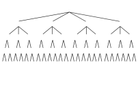
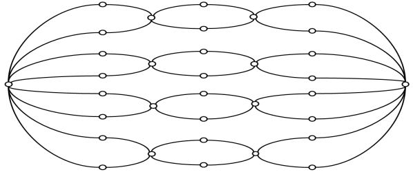
Figure 1: A read-once formula $f$ (on the left), which is a fan-in 4 OR of fan-in 3 $\mathrm{AND}$s of fan-in 2 $\mathrm{OR}$s of fan-in 2 $\mathrm{AND}$s, and the corresponding graph $G(f)$ (on the right).

Remark 4.

We note that if $f$ is a read-once monotone Boolean formula in which the bottom-level gates are $\mathrm{AND}$ gates and have fan-in at least two, then $G(f)$ is a simple graph and not a multigraph.

A simple inductive argument gives the following:

Observation 5.

If $f$ is a read-once monotone alternating formula with $r$ layers of $\mathrm{AND}$ gates of fan-ins $\alpha_{1},\dots,\alpha_{r}$, respectively, then every shortest path from $s$ to $t$ in the graph $G(f)$ has length exactly $\alpha_{1}\cdots\alpha_{r}.$ Furthermore, if $H$ is a subgraph of $G(f)$ that contains some $s$-to-$t$ path, then it contains a path of length $\alpha_{1}\cdots\alpha_{r}.$

As a corollary, we have:

Observation 6.

Every shortest path from $s$ to $t$ in $G(\mathsf{SkewedSipser}_{u,d})$ has length exactly $u^{d}.$

Given a read-once monotone formula $f$ over variables $x_{1},\dots,x_{n}$ and an assignment $z\in\{0,1\}^{n}$ to the variables $x_{1},\dots,x_{n}$, we define the graph $G(f,z)$ to be the (spanning) subgraph of $G(f)$ which has vertex set $V(f,z)=V(f)$ and edge set $E(f,z)$ defined as follows: each edge in $E(f)$ is present in $E(f,z)$ if and only if the corresponding coordinate of $z$ is set to 1. A simple inductive argument gives the following:

Observation 7.

Given a read-once monotone alternating formula with $r$ layers of $\mathrm{AND}$ gates of fan-ins $\alpha_{1},\dots,\alpha_{r}$, respectively, and an assignment $z\in\{0,1\}^{n}$, the graph $G(f,z)$ contains a path from $s$ to $t$ of length $\alpha_{1}\cdots\alpha_{r}$ if and only if $f(z)=1$.

From these observations we obtain the following connection between $\mathsf{SkewedSipser}_{u,d}$ and small-distance connectivity, which is key to our lower bound:

Corollary 3.1.

The multigraph $G(\mathsf{SkewedSipser}_{u,d},z)$ contains an $s$-to-$t$ path of length at most $u^{d}$ if and only if $\mathsf{SkewedSipser}_{u,d}(z)=1.$

Note that Corollary 3.1 and Theorem 2 together can be used to prove lower bounds for small-distance connectivity on multigraphs. One way to obtain lower bounds for simple graphs instead of multigraphs is by extending $\mathsf{SkewedSipser}_{u,d}$ with an extra layer of fan-in two AND gates next to the input variables, then relying on Remark 4. We use this simple observation and Theorem 2 to establish Theorem 1.

Theorem 1.

For any $k(n)\leq n^{1/{{5}}}$ and any $d=d(n)$, any depth-$d$ circuit computing $\mathit{STCONN}(k(n))$ must have size $n^{\Omega(k^{1/d}/d)}$. Furthermore, for any $k(n)\leq n$ and any $d=d(n)$, any depth-$d$ circuit computing $\mathit{STCONN}(k(n))$ must have size $n^{\Omega(k^{1/5d}/d)}$.

Proof.

We assume that $d<{2\log k/\log\log k}$ and $(k/2)^{1/d}\geq 2$ (observe that the claimed bound is trivial if $d\geq{2\log k/\log\log k}$ or $(k/2)^{1/d}<2$). Let

$$u_{0}=\left\lfloor(k/2)^{1/d}\right\rfloor.$$

Then we have $u_{0}\geq 2$ and $u_{0}=\Omega(k^{1/d})$. For convenience, let

$$k_{0}\stackrel{{\scriptstyle\rm def}}{{=}}u_{0}^{d}\leq k/2\quad\text{and}\quad n^{\prime}\stackrel{{\scriptstyle\rm def}}{{=}}\left\lfloor\frac{n}{2}\right\rfloor.$$ (1)

Further, let $w_{0}$ be the largest positive integer such that

$$(u_{0}w_{0})^{d}w_{0}^{{{33/100}}}\leq n^{\prime}.$$ (2)

Observe that, since $k\leq n^{1/5}$ and $d<2\log k/\log\log k$, as $n\to+\infty$ we have similarly $w_{0}\to+\infty$. Our choice of $w_{0}$ also implies that $w_{0}$ satisfies

$$u_{0}^{d}(w_{0}+1)^{d+33/100}>n^{\prime}.$$

Let $n_{0}\stackrel{{\scriptstyle\rm def}}{{=}}(u_{0}w_{0})^{d}w_{0}^{{{33/100}}}$. Then from $d<2\log k/\log\log k$ and $w_{0}\rightarrow+\infty$ we have

$$n_{0}\geq u_{0}^{d}\left(\frac{w_{0}+1}{2}\right)^{d+\frac{33}{100}}\!=\,\Omega(n/2^{d})=\omega(n^{0.99}).$$

Combining this with $k\leq n^{1/5}$ and $k_{0}\leq k/2$ we have that $k_{0}=o(n_{0}^{20/99})$ and $n_{0}\geq k_{0}^{4.9}$ when $n$ is sufficiently large.

We define a variant of our $\mathsf{SkewedSipser}_{u,d}$ formula so we can rely on Remark 4 and work directly with simple graphs instead of multigraphs. More precisely, let $\smash{\mathsf{SkewedSipser}^{\dagger}_{u_{0},w_{0},d}}$ be analogous to $\mathsf{SkewedSipser}_{u,d}$ with parameters $u_{0}$ (AND gate fan-in), $w_{0}$ (OR gate fan-in), and $d$ but containing an extra layer of fan-in 2 AND gates at the bottom connected to a new set of input variables. In other words, this is a depth $2d+2$ read-once alternating formula with twice the number of input variables of our original $\mathsf{SkewedSipser}$ formula (each input variable of $\mathsf{SkewedSipser}$ becomes an AND gate connected to two new fresh variables). Since $\mathsf{SkewedSipser}_{u_{0},d}$ can be obtained by restricting $\smash{\mathsf{SkewedSipser}^{\dagger}_{u_{0},w_{0},d}}$ appropriately (i.e. by setting to 1 a single variable in every new pair of variables) a lower bound on the circuit complexity of $\mathsf{SkewedSipser}$ immediately implies the same lower bound for $\smash{\mathsf{SkewedSipser}^{\dagger}}$.

In order to obtain a lower bound via Theorem 2, we need that $w_{0}^{{{33/100}}}\geq u_{0}$. This is equivalent to having $\smash{n_{0}\geq u_{0}^{{{133d/33+{{1}}}}}}$, which follows from $d\geq 2$ (we may assume $d\geq 2$ since no depth-1 circuit, i.e. single $\mathrm{AND}$ or $\mathrm{OR}$ gate, can compute $\mathit{STCONN}(k(n))$) and $n_{0}\geq k_{0}^{4.9}$ since

$$n_{0}\geq{{k_{0}^{{4.9}}}}>k_{0}^{{{133/33+{{1/2}}.}}}$$

Consequently, we can apply Theorem 2 to $\mathsf{SkewedSipser}_{u_{0},d}$, and it follows from our discussion above that any depth-$d$ circuit computing $\smash{\mathsf{SkewedSipser}^{\dagger}_{u_{0},w_{0},d}}$ must have size at least

$$n_{0}^{\Omega(u_{0}/d)}=n^{\Omega(k^{1/d}/d)}.$$ (3)

In the rest of the proof we translate (3) into a lower bound for $\mathit{STCONN}(k(n))$. Following the explanation given above, we consider the simple graph $G(\mathsf{SkewedSipser}^{\dagger})$ with appropriate parameters. Since $u_{0}^{d}\leq k/2$, it follows from the same argument used to establish Corollary 3.1 that the graph $\smash{G(\mathsf{SkewedSipser}^{\dagger}_{u_{0},w_{0},d},z)}$ contains an $s$-to-$t$ path of length at most $2u_{0}^{d}\leq k$ if and only if we have $\smash{\mathsf{SkewedSipser}^{\dagger}_{u_{0},w_{0},d}(z)=1}$. Because $\smash{G(\mathsf{SkewedSipser}^{\dagger}_{u_{0},w_{0},d})}$ has no isolated vertices and has $n_{0}$ edges, it contains at most $2n_{0}\leq 2n^{\prime}\leq n$ vertices by (1) and (2). Thus, a circuit $\mathcal{C}$ that computes $\mathit{STCONN}(k(n))$ on undirected simple graphs on $n$ vertices can also be used to compute the formula $\smash{\mathsf{SkewedSipser}^{\dagger}_{u_{0},w_{0},d}}$, and (3) yields that $\mathcal{C}$ must have size $n^{\Omega(k^{1/d}/d)}$. This completes the first part of Theorem 1.

It remains to prove the lower bound for $\mathit{STCONN}({{k^{\prime}}}(n))$ with $n^{1/5}<k^{\prime}(n)\leq n$. For this, let ${{k}}(n)\stackrel{{\scriptstyle\rm def}}{{=}}n^{1/{{5}}}$. We have established above that computing $\mathit{STCONN}(k(n))$ on subgraphs of $\smash{G(\mathsf{SkewedSipser}^{\dagger}_{u_{0},w_{0},d})}$ using depth-$d$ circuits requires size $n^{\Omega(k^{1/d}/d)}$. However, a subgraph of $\smash{G(\mathsf{SkewedSipser}^{\dagger}_{u_{0},w_{0},d})}$ contains an $s$-to-$t$ path of length at most $k(n)$ if and only if it contains a path from $s$ to $t$ of length at most $k^{\prime}(n)$ (Observation 5). Consequently, any circuit $\mathcal{C}$ that computes $\mathit{STCONN}(k^{\prime}(n))$ on general $n$-vertex graphs can be used to compute $\mathit{STCONN}(k(n))$ on subgraphs of $G(\mathsf{SkewedSipser}^{\dagger}_{u_{0},w_{0},d})$ (by setting some input edges to 0). In particular, $\mathcal{C}$ must have size

$$n^{\Omega(k^{1/d}/d)}=n^{\Omega(n^{1/5d}/d)}=n^{\Omega({{k^{\prime}}}^{1/5d}/d)}.$$

This completes the second part of Theorem 1. ∎

Remark 8.

It is not hard to see that our reduction in fact also captures other natural graph problems such as directed $k$-path (“Is there a directed path of length $k(n)$ in $G$?”) and directed $k$-cycle (“Is there a directed cycle of length $k(n)$ in $G$?”), and hence the lower bounds of Theorem 1 apply to these problems as well. This suggests the possibility of similarly obtaining other lower bounds from (variants of) depth hierarchy theorems for Boolean circuits, and we leave this as an avenue for further investigation.

4 The Random Projection

In this section we define our random projections, which will be crucial in the proof of Theorem 2. First, we introduce notation to manipulate the first two layers of $\mathsf{SkewedSipser}_{u,d}$.

Definition 9.

For $2\leq u\leq w$, we define $\mathsf{CNFSipser}_{u}$ to be the Boolean function computed by the following monotone read-once formula:

• The top gate is an $\mathrm{AND}$ gate and the bottom-layer gates are $\mathrm{OR}$ gates.

• The top $\mathrm{AND}$ gate has fanin $u$.

• The bottom-layer $\mathrm{OR}$ gates all have fan-in ${{w^{33/100}}}$.

For $\mathsf{SkewedSipser}_{u,d}$ and each $\ell\in[d+1]$, we write $\mathrm{OR}^{(\ell)}$ to denote an $\mathrm{OR}$ gate that is in the $\ell$-th level of $\mathrm{OR}$ gates away from the input variables and similarly write $\smash{\mathrm{AND}^{(\ell)}}$ to denote an $\mathrm{AND}$ gate that is in the $\ell$-th level of $\mathrm{AND}$ gates away from the input variables. So the root of $\mathsf{SkewedSipser}_{u,d}$ is the only $\smash{\mathrm{OR}^{(d+1)}}$ gate; each $\smash{\mathrm{AND}^{(\ell)}}$ gate has $u$ many $\smash{\mathrm{OR}^{(\ell)}}$ gates as its inputs; each $\smash{\mathrm{AND}^{(1)}}$ gate of $\mathsf{SkewedSipser}_{u,d}$ computes a disjoint copy of $\mathsf{CNFSipser}_{u}$.

Next we introduce an addressing scheme for gates and variables of $\mathsf{SkewedSipser}_{u,d}$.

Addressing scheme.

Viewing $\mathsf{SkewedSipser}_{u,d}$ as a tree (with its leaves being variables and the rest being $\mathrm{AND},\mathrm{OR}$ gates), we index its nodes (gates or variables) by addresses as follows. The root (gate) is indexed by $\varepsilon$, the empty string. The $j$-th child of a node is indexed by the address of its parent concatenated with $j$. Thus, the variables of $\mathsf{SkewedSipser}_{u,d}$ are indexed by addresses

$$A(d):=\Big{\{}(b_{0},a_{1},b_{1},\ldots,a_{d},b_{d})\colon a_{i}\in[u],b_{0},\ldots,b_{d-1}\in[w],b_{d}\in[{{w^{33/100}}}]\Big{\}}.$$

Block and section decompositions.

We will refer to the set of $u{{w^{33/100}}}$ addresses of variables below an $\mathrm{AND}^{(1)}$ gate as a block, and the set of ${{w^{33/100}}}$ addresses of variables below an $\mathrm{OR}^{(1)}$ gate as a section.

It will be convenient for us to view the set of all variable addresses $A(d)$ as

$$A(d)=B(d)\times A^{\prime},\text{~{}where}$$

$$B(d)=\big{\{}(b_{0},a_{1},b_{1}\ldots,a_{d-1},b_{d-1})\colon a_{i}\in[u],b_{i}\in[w]\big{\}}\ \ \ \text{and}\ \ \ A^{\prime}=[u]\times[{{w^{33/100}}}].$$

Here $B(d)$ can be viewed as the set of addresses of the $\mathrm{AND}^{(1)}$ gates of $\mathsf{SkewedSipser}_{u,d}$, and $A^{\prime}$ can be viewed as the set of variable addresses of $\mathsf{CNFSipser}_{u}$ computed by each such gate (following the same addressing scheme).

More formally, for a fixed $\beta\in B(d)$ we call the set of addresses

$$A(d,\beta)\stackrel{{\scriptstyle\rm def}}{{=}}\big{\{}(\beta,\tau)\colon\tau\in A^{\prime}\big{\}}$$

a block of $A(d)$; these are the addresses of variables below the $\mathrm{AND}^{(1)}$ gate specified by $\beta$. Thus, $A(d)$ is the disjoint union of $w(uw)^{d-1}$ many blocks, each of cardinality $|A^{\prime}|=u{{w^{33/100}}}$.

For a fixed $\beta\in B(d)$ and $a\in[u]$, we call the set of addresses

$${{A(d,\beta,a)}}\stackrel{{\scriptstyle\rm def}}{{=}}\big{\{}(\beta,a,b)\colon b\in[{{w^{33/100}}}]\big{\}}$$

a section of $A(d)$; these are the addresses of variables below the $\mathrm{OR}^{(1)}$ gate specified by ${{(\beta,a)}}$. Each block $A(d,\beta)$ is the disjoint union of $u$ many sections, each of cardinality ${{w^{33/100}}}$.

To summarize, the set of addresses of variables $A(d)$ can be decomposed into $w(uw)^{d-1}$ many blocks $A(d,\beta)$ (corresponding to the $\mathrm{AND}^{(1)}$ gates), $\beta\in B(d)$, and each such block can be further decomposed into $u$ many sections $A(d,\beta,a)$ (corresponding to its $u$ input $\mathrm{OR}^{(1)}$ gates), $a\in[u]$.

Accordingly we also decompose $A^{\prime}$, the set of variable addresses of $\mathsf{CNFSipser}_{u}$, into sections

$$A^{\prime}(a)\stackrel{{\scriptstyle\rm def}}{{=}}\big{\{}(a,b)\colon b\in[{{w^{33/100}}}]\big{\}},\quad\text{for $a\in[u]$}.$$

The following fact is trivial given the definition of $\mathsf{CNFSipser}_{u}$. (Below and subsequently, we use “$\varrho$” to denote a restriction to the variables of $\mathsf{CNFSipser}$ and “$\rho$” to denote a restriction to the variables of $\mathsf{SkewedSipser}$.)

Fact 4.1.

For any $a\in[u]$ and restriction $\varrho\in\{0,1,\ast\}^{A^{\prime}}$ that sets all variables in the $a$-th section $A^{\prime}(a)$ to $0$, i.e., $\varrho_{\tau}=0\text{ for all $\tau\in A^{\prime}(a)$},$ we have that $\mathsf{CNFSipser}_{u}\upharpoonright\varrho\equiv 0$.

Now we define our random projection operator $\mathrm{proj}_{\boldsymbol{\rho}}(\cdot)$.

Definition 10 (Projection operators).

Given a restriction $\rho\in\{0,1,\ast\}^{A(d)}$, the projection operator $\mathrm{proj}_{\rho}$ maps a function $\smash{f\colon\{0,1\}^{A(d)}\rightarrow\{0,1\}}$ to a function $\smash{\mathrm{proj}_{\rho}(f)\colon\{0,1\}^{B(d)}\rightarrow\{0,1\}}$, where

$$\big{(}\mathrm{proj}_{\rho}(f)\big{)}(y)=f(x),\quad\text{where}\ x_{\beta,\tau}\stackrel{{\scriptstyle\rm def}}{{=}}\ \begin{cases}y_{\beta}&\text{if $\rho_{\beta,\tau}=\ast$}\\ \rho_{\beta,\tau}&\text{if $\rho_{\beta,\tau}\in\{0,1\}$.}\end{cases}$$

For convenience, we sometimes write $\mathrm{proj}(f\upharpoonright\rho)$ instead of $\mathrm{proj}_{\rho}(f)$.

Remark 11.

The following interpretation of the projection operator will come in handy. Given a restriction $\rho\in\{0,1,\ast\}^{A(d)}$, if $f$ is computed by a circuit $C$, then $\mathrm{proj}_{\rho}(f)$ is computed by a circuit $C^{\prime}$ obtained from $C$ by replacing every occurrence of $x_{\beta,\tau}$ by $y_{\beta}$ if $\rho_{\beta,\tau}=\ast$, or by $\rho_{\beta,\tau}$ if $\rho_{\beta,\tau}\in\{0,1\}$.

The crux of our random projection operator $\mathrm{proj}_{\boldsymbol{\rho}}(\cdot)$ is then a distribution $\mathcal{D}^{(d)}_{u}$ over restrictions $\smash{\{0,1,\ast\}^{A(d)}}$ to the variables $\{x_{\beta,\tau}:(\beta,\tau)\in A(d)\}$, from which ${\boldsymbol{\rho}}$ is drawn. To this end, we consider the block decomposition $B(d)\times A^{\prime}$ of $A(d)$, and $\smash{{\boldsymbol{\rho}}\leftarrow\mathcal{D}^{(d)}_{u}}$ is obtained by drawing independently, for each block $\beta\in B(d)$, a restriction ${\boldsymbol{\rho}}_{\beta}$ from a distribution $\mathcal{D}_{u}$ over $\{0,1,\ast\}^{A^{\prime}}$ to be defined below.

Definition 12 (Distributions $\mathcal{D}_{u}$ and $\mathcal{D}_{u}^{(d)}$).

The distribution $\mathcal{D}_{u}=\mathcal{D}_{u}(q)$ over $\{0,1,\ast\}^{A^{\prime}}$ is parameterized by a probability $q\in(0,1)$. A draw of a restriction $\boldsymbol{\varrho}$ from $\mathcal{D}_{u}$ is generated as follows:

• With probability $q$, output $\boldsymbol{\varrho}=\{\ast\}^{A^{\prime}}$ (i.e. the restriction fixes no variables).

• Otherwise (with probability $1-q$), we draw $\boldsymbol{a}\leftarrow[u]$ (a random section) and $\boldsymbol{z}\leftarrow\{0,1\}$ (a random bit) independently and uniformly at random, and output $\boldsymbol{\varrho}$ where for each $\tau\in A^{\prime}$,

  $$\boldsymbol{\varrho}_{\tau}=\begin{cases}\boldsymbol{z}&\text{if $\tau\in A^{\prime}(\boldsymbol{a})$}\\ 1-\boldsymbol{z}&\text{otherwise.}\end{cases}$$

  Note that in this case $\boldsymbol{\varrho}$ is distributed uniformly among $2u$ many binary strings in $\{0,1\}^{{{A^{\prime}}}}$. These strings are “section-monochromatic”, with $u-1$ of the sections taking on entirely the same value ${{1-\boldsymbol{z}}}$ and the one remaining section $\boldsymbol{a}$ taking entirely the other “rare” value ${{\boldsymbol{z}}}$.

As described above, a draw of ${\boldsymbol{\rho}}\in\{0,1,\ast\}^{B(d)\times A^{\prime}}$ from $\mathcal{D}_{u}^{(d)}=\mathcal{D}_{u}^{(d)}(q)$ is obtained by independently drawing ${\boldsymbol{\rho}}_{\beta}\leftarrow\mathcal{D}_{u}=\mathcal{D}_{u}(q)$ for each block $\beta\in B(d).$

The following observation about $\mathrm{supp}(\mathcal{D}^{(d)}_{u})$ will be useful for us:

Remark 13.

A restriction $\rho\in\{0,1,\ast\}^{B(d)\times A^{\prime}}$ is in the support of $\mathcal{D}^{(d)}_{u}$ iff for every block $\beta\in B(d)$, $\rho_{\beta}$ is either $\{\ast\}^{A^{\prime}}$, or there exists exactly one section $a\in[u]$ such that $\rho_{\beta,\tau}=0$ if $\tau\in A^{\prime}(a)$ and $1$ otherwise, or there exists exactly one section $a\in[u]$ such that $\rho_{\beta,\tau}=1$ if $\tau\in A^{\prime}(a)$ and $0$ otherwise.

Therefore, if $T$ is a term of width at most $u-1$ such that for all blocks $\beta\in B(d)$, the variables from block $\beta$ that occur in $T$ all occur with the same sign, then $T$ can be satisfied by a restriction in the support of $\smash{\mathcal{D}^{(d)}_{u}}$ (i.e., $T\upharpoonright\rho\equiv 1$ for some $\smash{\rho\in\mathrm{supp}(\mathcal{D}^{(d)}_{u})}$). (Note that this crucially uses the fact that $T$ has width at most $u-1$, and in particular does not contain variables from all $u$ sections of any block $\beta$. Also note that the inverse of this is not true, e.g., consider $T=x_{\beta,\tau}\land\neg\,x_{\beta,\tau^{\prime}}$ with $\tau$ and $\tau^{\prime}$ from two different sections.)

5 Projection Switching Lemma

Our goal now is to prove the following projection switching lemma for (very) small width DNFs:

Theorem 14 (Projection Switching Lemma).

For $2\leq u\leq w$, let $F$ be an $r$-DNF over the variables $\{x_{\beta,\tau}\}$, ${(\beta,\tau)\in A(d)}$, where $r\leq u-1$. Then for all $s\geq 1$ and $q\in(0,1)$, we have

$$\mathop{{\bf Pr}\/}_{{\boldsymbol{\rho}}\leftarrow\mathcal{D}_{u}^{(d)}{{(q)}}}\Big{[}\hskip 1.70709pt\text{$\mathrm{proj}_{\boldsymbol{\rho}}(F)$ has decision tree depth $\geq s$}\hskip 0.85355pt\Big{]}\leq\left(\frac{8qru}{1-q}\right)^{\!s}.$$

Notice that while $F$ is an $r$-DNF over formal variables $\{x_{\beta,\tau}\colon(\beta,\tau)\in A(d)\}$, we will bound the decision tree depth of $\mathrm{proj}_{\boldsymbol{\rho}}(F)$, a function over the new formal variables $\{y_{\beta}\colon\beta\in B(d)\}$.

Remark 15.

Projections will play a key role in the proof. Consider a term of the form $T=x_{\beta,\tau}\wedge\neg\,x_{\beta,\tau^{\prime}}$ for some $\tau\neq\tau^{\prime}$, and suppose our $\rho$ from $\mathcal{D}^{(d)}_{u}$ is such that $\rho_{\beta,\tau}=\rho_{\beta,\tau^{\prime}}=\ast$. In this case we have $T\upharpoonright\rho=x_{\beta,\tau}\wedge\neg\,x_{\beta,\tau^{\prime}},$ i.e., the term survives the restriction $\rho$, but $\mathrm{proj}_{\rho}(T)=y_{\beta}\wedge\neg\,y_{\beta}\equiv 0,$ i.e., the term is killed by $\mathrm{proj}_{\rho}$. Our proof will crucially leverage simplifications of this sort.

Remark 16.

The parameters of Theorem 14 are quite delicate in the sense that the statement fails to hold for DNFs of width $u$. To see this, consider $\mathsf{SkewedSipser}_{u,{{d}}}$ with $d=1$, a depth-$3$ formula that can also be written as a $u$-DNF. Then by Corollary 6.2 (to be introduced in Section 6), we have that for $\smash{{\boldsymbol{\rho}}\leftarrow\mathcal{D}^{(1)}_{u}(q)}$ with $\smash{q=w^{-669/1000}}$, the function $\smash{\mathrm{proj}_{\boldsymbol{\rho}}(\mathsf{SkewedSipser}_{u,1})}$ contains a $\smash{{{w^{33/100}}}}$-way $\mathrm{OR}$ as a subfunction — and hence has decision tree depth at least ${{w^{33/100}}}$ — with probability $1-o(1)$. So while the statement of Theorem 14 holds for $(u-1)$-DNFs, it does not hold for $u$-DNFs when $u=o(w^{{{669/2000}}})$ and $w\to\infty$.

Remark 17.

We observe that the conclusion of Theorem 14 still holds if the condition “$F$ is an $r$-CNF” replaces “$F$ is an $r$-DNF.” This can be shown either by a straightforward adaptation of our proof, or via a reduction to the DNF case using duality, the invariance of our distribution of random projections under the operation of flipping each bit, and the fact that decision tree depth does not change when input variables and output value are negated.

5.1 Canonical decision tree

Given an $r$-DNF $F$ over variables $\{x_{\beta,\tau}:(\beta,\tau)\in A(d)\}$ and a restriction $\rho\in\{0,1,\ast\}^{A(d)}$, $\mathrm{proj}_{\rho}(F)$ is a function over the new variables $\{y_{\beta}:\beta\in B(d)\}$. We assume a fixed but arbitrary ordering on the terms in $F$, and the variables within terms. The canonical decision tree $\mathsf{CanonicalDT}(F,\rho)$ that computes $\mathrm{proj}_{\rho}(F)$ is defined inductively as follows.

CanonicalDT${{(F,\rho)}}$ :

1. If ${{\mathrm{proj}_{\rho}(F)}}\equiv 0$ or $1$, output $0$ or $1$, respectively.

2. Otherwise, let $T$ be the first term in $F$ such that $T\upharpoonright\rho$ is non-constant and $T\upharpoonright\rho\rho^{\prime}\equiv 1$ for some $\smash{\rho^{\prime}\in\mathrm{supp}(\mathcal{D}_{u}^{(d)})}$. We observe that such a term must exist, or the procedure would have halted at step 0 above and not reached the current step 1.

   To see this, first note that certainly there must exist a term $T^{\prime}$ such that $T^{\prime}\upharpoonright\rho$ is non-constant since otherwise $F\upharpoonright\rho$ is constant (and likewise $\mathrm{proj}_{\rho}(F)$). We furthermore claim that among these terms $T^{\prime}$, there must exist one such that $T^{\prime}\upharpoonright\rho$ is satisfiable by some $\smash{\rho^{\prime}\in\mathrm{supp}(\mathcal{D}_{u}^{(d)})}$, i.e. $T^{\prime}\upharpoonright\rho\rho^{\prime}\equiv 1$. To prove this, suppose that each of these terms $T^{\prime}$ satisfies that $T^{\prime}\upharpoonright\rho$ is non-constant and there exists no restriction $\smash{\rho^{\prime}\in\mathrm{supp}(\mathcal{D}^{(d)}_{u})}$ such that $T^{\prime}\upharpoonright\rho\rho^{\prime}\equiv 1$. By Remark 13 (and our assumption that $r\leq u-1$), $T^{\prime}\upharpoonright\rho$ must contain two literals from the same block occurring with opposite signs, i.e., $x_{\beta,\tau}$ and $\neg\,x_{\beta,\tau^{\prime}},$ for some $\beta\in B(d)$. In this case, we have that $\mathrm{proj}_{\rho}(T^{\prime})$ contains both $y_{\beta}$ and $\neg\,y_{\beta}$ and hence $\mathrm{proj}_{\rho}(T^{\prime})\equiv 0$. But if each such term $T^{\prime}$ has $\mathrm{proj}_{\rho}(T^{\prime})\equiv 0$, then $\mathrm{proj}_{\rho}(F)\equiv 0$ and the procedure would have halted at step (0).

3. Define

   $$\eta=\big{\{}\beta\in B(d)\colon x_{\beta,\tau}\text{~{}or~{}}\neg\,x_{\beta,\tau}\text{ occurs in $T\upharpoonright\rho$ for some $\tau$}\big{\}}$$

   Our canonical decision tree will then query variables $y_{\beta}$, $\beta\in\eta$ exhaustively, i.e., we grow a complete binary tree of depth $|\eta|$; we will refer to $T$ as the term of this tree.

4. For every assignment $\pi\in\{0,1\}^{\eta}$ to variables $y_{\beta}$, $\beta\in\eta$ (equivalently, every path through the complete binary tree of depth $\smash{|\eta|}$), we recurse on $\mathsf{CanonicalDT}(F,\rho(\eta\mapsto\pi))$, where we use $(\eta\mapsto\pi)\in\{0,1,\ast\}^{A(d)}$ to denote the following restriction:

   $$(\eta\mapsto\pi)_{\beta,\tau}=\begin{cases}{{\pi_{\beta}}}&\text{if $\beta\in\eta$}\\ \ast&\text{otherwise,}\end{cases}\quad\text{for all $\beta\in B(d)$ and $\tau\in A^{\prime}$}.$$ (4)

Proposition 5.1.

For every $\rho\in\{0,1,\ast\}^{A(d)}$, we have that $\mathsf{CanonicalDT}(F,\rho)$ computes $\mathrm{proj}_{\rho}(F)$.

While $\mathsf{CanonicalDT}$ is well defined for all $\rho$, we shall mostly be interested in $\rho\in\mathrm{supp}(\mathcal{D}^{(d)}_{u})$.

5.2 Proof of Theorem 14

Let

$$\mathcal{B}\stackrel{{\scriptstyle\rm def}}{{=}}\big{\{}\rho\in\mathrm{supp}(\mathcal{D}^{(d)}_{u})\colon\text{decision tree depth of\ }\mathsf{CanonicalDT}(F,\rho)\geq s\big{\}}$$

be the set of bad restrictions, To prove Theorem 14, it suffices to bound ${\operatorname{{\bf Pr}}_{{\boldsymbol{\rho}}\leftarrow\mathcal{D}^{(d)}_{u}{{(q)}}}[\hskip 0.85355pt{\boldsymbol{\rho}}\in\mathcal{B}\hskip 0.85355pt]},$ the total weight of $\mathcal{B}$ under $\mathcal{D}^{(d)}_{u}{{(q)}}$. Following Razborov’s strategy (see [Bea95] for more details), we will construct a map

$$\theta\colon\mathcal{B}\rightarrow\{0,1,\ast\}^{A(d)}\times\{0,1\}^{s}\times\{0,1\}^{s(\log r+1)},$$

with the following two key properties:

1. (injection) $\theta(\rho)\neq\theta(\rho^{\prime})$ for any two distinct restrictions $\rho,\rho^{\prime}\in\mathcal{B}$;

2. (weight increase) Let $\theta_{1}(\rho)\in\{0,1,\ast\}^{A(d)}$ denote the first component of $\theta(\rho)$. Then

   $$\frac{\operatorname{{\bf Pr}}[\hskip 0.85355pt{\boldsymbol{\rho}}=\theta_{1}(\rho)\hskip 0.85355pt]}{\operatorname{{\bf Pr}}\hskip 0.85355pt[{\boldsymbol{\rho}}=\rho\hskip 0.85355pt]}\geq\Gamma,\quad\text{for all $\rho\in\mathcal{B}$},$$ (5)

   where $\Gamma={{((1-q)/2qu)^{s}}}$ is “large”.

Assuming such a map $\theta$ exists (below we describe its construction and prove the two properties stated above), Theorem 14 follows from a simple combinatorial argument.

Proof of Theorem 14.

Fix a pair $O\in\{0,1\}^{s}\times\{0,1\}^{s(1+\log r)}$ and let

$$\mathcal{B}_{O}=\big{\{}\rho\in\mathcal{B}\colon\big{(}\theta_{2}(\rho),\theta_{3}(\rho)\big{)}=O\big{\}}\subseteq\mathcal{B},$$

where we use $\theta_{2}(\rho)$ and $\theta_{3}(\rho)$ to denote the second and third components of $\theta(\rho)$, respectively.

Then we have that

$$\mathop{{\bf Pr}\/}[\hskip 0.85355pt{\boldsymbol{\rho}}\in\mathcal{B}_{O}\hskip 0.85355pt]=\sum_{\rho\in\mathcal{B}_{O}}\operatorname{{\bf Pr}}[\hskip 0.85355pt{\boldsymbol{\rho}}=\rho\hskip 0.85355pt]\leq(1/\Gamma)\cdot\sum_{\rho\in\mathcal{B}_{O}}\operatorname{{\bf Pr}}[\hskip 0.85355pt{\boldsymbol{\rho}}=\theta_{1}(\rho)\hskip 0.85355pt]\leq 1/\Gamma.$$

Here the first inequality uses (5) and the second inequality uses the property of $\theta$ being an injection: we have that $\theta_{1}(\rho)\neq\theta_{1}(\rho^{\prime})$ for any two distinct $\rho,\rho^{\prime}\in\mathcal{B}_{O}$ (recall that $\theta_{2}(\rho)=\theta_{2}(\rho^{\prime})$ and $\theta_{3}(\rho)=\theta_{3}(\rho^{\prime})$), and therefore $\sum_{\rho\in\mathcal{B}_{O}}\operatorname{{\bf Pr}}[\hskip 0.85355pt{\boldsymbol{\rho}}=\theta(\rho)_{1}\hskip 0.85355pt]\leq 1$. Summing up over all possible $O$’s, we have

$$\operatorname{{\bf Pr}}[\hskip 0.85355pt{\boldsymbol{\rho}}\in\mathcal{B}\hskip 0.85355pt]=\sum_{O}\operatorname{{\bf Pr}}[\hskip 0.85355pt{\boldsymbol{\rho}}\in\mathcal{B}_{O}\hskip 0.85355pt]\leq 2^{s}\cdot(2r)^{s}\cdot\big{(}2qu/(1-q)\big{)}^{s}=\big{(}8qru/(1-q)\big{)}^{s},$$

and this concludes the proof of Theorem 14. ∎

The rest of the section is organized as follows. We construct the map $\theta$ in Section 5.3. Then we show that it is an injection in Section 5.4, by showing that one can decode $\rho$ from $\theta(\rho)$ uniquely for any $\rho\in\mathcal{B}$. Finally we prove the weight increase, i.e., (5) in Section 5.5.

5.3 Encoding

Let $\rho\in\mathcal{B}$ be a bad restriction. Let $\pi^{*}$ be the lexicographically first path of length at least $s$ in the decision tree $\mathsf{CanonicalDT}(F,\rho)$ (witnessing the badness of $\rho$), and $\pi$ be its truncation at length $s$. Then $\theta_{2}(\rho)$ is defined to be $\textrm{binary}(\pi)\in\{0,1\}^{s}$, the binary representation of $\pi$, i.e., $\pi_{i}\in\{0,1\}$ is the evaluation of the $i$th $y$-variable along $\pi$.

Recall that $\mathsf{CanonicalDT}(F,\rho)$ is composed of a collection of complete binary trees, one for each recursive call of $\mathsf{CanonicalDT}$. Let $R_{1},\ldots,R_{s^{\prime}}$ for some $1\leq s^{\prime}\leq s$ denote the sequence of complete binary trees that $\pi$ visits, with $R_{1}$ sharing the same root as $\mathsf{CanonicalDT}(F,\rho)$ and $\pi$ ending in $R_{s^{\prime}}$. (Here $s^{\prime}\geq 1$ because $s\geq 1$.) We also use $T_{i}$ to denote the term of tree $R_{i}$, for each $i\in[s^{\prime}]$.

For each $i\in[s^{\prime}-1]$, we let

$$\eta_{i}=\big{\{}\beta\in B(d):y_{\beta}\ \text{is queried in tree $R_{i}$}\big{\}},$$

and for the special case of $i=s^{\prime}$, we let

$$\eta_{s^{\prime}}=\big{\{}\beta\in B(d):y_{\beta}\ \text{is queried in tree $R_{s^{\prime}}$ before the end of $\pi$}\big{\}}.$$ (6)

For each $i\in[s^{\prime}]$, $\pi$ induces a binary string $\pi^{(i)}\in\{0,1\}^{\eta_{i}}$, where $\pi^{(i)}_{\beta}$ for each $\beta\in\eta_{i}$ is set to be the evaluation of $y_{\beta}$ along $\pi$ (in tree $R_{i}$). Note that $T_{i}$ is the $i$-th term processed by $\mathsf{CanonicalDT}(F,\rho)$ along the bad path $\pi$ and equivalently, $T_{i}$ is the first term processed by

$$\mathsf{CanonicalDT}\big{(}F,\rho(\eta_{1}\mapsto\pi^{(1)})\cdots(\eta_{i-1}\mapsto\pi^{(i-1)})\big{)},$$

where $(\eta_{j}\mapsto\pi^{(j)})$ is a restriction defined as in (4). So $T_{i}$ is the first term in $F$ such that

$$T_{i}\upharpoonright\rho(\eta_{1}\mapsto\pi^{(1)})\cdots(\eta_{i-1}\mapsto\pi^{(i-1)})$$

is non-constant and

$$T_{i}\upharpoonright\rho(\eta_{1}\mapsto\pi^{(1)})\cdots(\eta_{i-1}\mapsto\pi^{(i-1)})\rho^{\prime}\equiv 1,\quad\text{for some $\rho^{\prime}\in\mathrm{supp}(\mathcal{D}^{(d)}_{u})$.}$$

At a high level, $\theta_{1}(\rho)$ and $\theta_{3}(\rho)$ are defined as follows. The third component

$$\theta_{3}(\rho)=\mathrm{encode}(\eta_{1})\circ\cdots\circ\mathrm{encode}(\eta_{s^{\prime}})\in\{0,1\}^{s(1+\log r)}$$

is the concatenation of $s^{\prime}$ binary strings, where each $\mathrm{encode}(\eta_{i})$ is a concise representation of $\eta_{i}$. In particular, we are able to recover $\eta_{i}$ given both $\mathrm{encode}(\eta_{i})$ and $T_{i}$. We describe the encoding of $\eta_{i}$ in Section 5.3.1. For the first component we have

$$\theta_{1}(\rho)=\rho\sigma^{(1)}\cdots\sigma^{(s^{\prime})}\in\{0,1,\ast\}^{A(d)},$$

where each $\sigma^{(i)}\in\{0,1,\ast\}^{A(d)}$ is a restriction and $\rho\sigma^{(1)}\cdots\sigma^{(s^{\prime})}$ is their composition (note that each of these $s^{\prime}+1$ restrictions, like the overall composition, belongs to $\{0,1,\ast\}^{A(d)}$). We define the $\sigma^{(i)}$’s in Section 5.3.2.

5.3.1 Encoding $\eta_{i}$

Fix an $i\in[s^{\prime}]$. Let $\eta_{i}=\{\beta_{1},\ldots,\beta_{t}\}$ for some $t\geq 1$, with $\beta_{j}$’s ordered lexicographically. It follows from the definition of $\eta_{i}$ that every $\beta_{j}$ appears in $T_{i}$, meaning that either $x_{\beta,\tau}$ or $\neg\,x_{\beta,\tau}$ appears in $T_{i}$ for some $\tau\in A^{\prime}$.

Instead of encoding each $\beta_{j}$ directly using its binary representation, we use $\log r$ bits to encode the index of the first $x_{\beta,\cdot}$ or $\neg\,x_{\beta,\cdot}$ variable that occurs in $T_{i}$. Here $\log r$ bits suffice because $T_{i}$ has at most $r$ variables. Also recall that we fixed an ordering on the variables of each term, so indices of variables in $T_{i}$ are well defined. We let $\mathrm{location}(\beta_{j})$ denote the $\log r$ bits for $\beta_{j}$. We also append it with one additional bit to indicate whether $\beta_{j}$ is the last element in $\eta_{i}$. More formally, we write

$$\mathrm{encode}(\eta_{i})=\mathrm{location}(\beta_{1})\circ 0\circ\mathrm{location}(\beta_{2})\circ 0\circ\cdots\circ\mathrm{location}(\beta_{t})\circ 1\in\{0,1\}^{|\eta_{{{i}}}|(1+\log r)}.$$

We summarize properties of $\theta_{3}(\rho)$ below:

Proposition 5.2.

Given ${{\theta_{3}}}(\rho)$, one can recover uniquely $s^{\prime}$ and $\mathrm{encode}(\eta_{1}),\ldots,\mathrm{encode}(\eta_{s^{\prime}})$. Furthermore, given $\mathrm{encode}(\eta_{i})$ and $T_{i}$ for some $i\in[s^{\prime}]$, one can recover uniquely $\eta_{i}$.

5.3.2 The $\sigma^{(i)}$ restriction

We now define $\sigma^{(i)}$ for a general $i\in[s^{\prime}]$. For ease of notation we define the restriction

$$\rho^{(i-1)}\stackrel{{\scriptstyle\rm def}}{{=}}\rho(\eta_{1}\mapsto\pi^{(1)})\cdots(\eta_{i-1}\mapsto\pi^{(i-1)})\in\{0,1,\ast\}^{A(d)}.$$

Note that $\rho^{(0)}=\rho$. Recalling our $\mathsf{CanonicalDT}$ algorithm and the definition of $T_{i}$ as the $i$-th term processed by $\mathsf{CanonicalDT}(F,\rho)$, we have that $T_{i}$ is the first term in $F$ such that $T_{i}\upharpoonright\rho^{(i-1)}$ is non-constant and $\smash{T_{i}\upharpoonright\rho^{(i-1)}\rho^{\prime}\equiv 1}$ for some $\smash{\rho^{\prime}\in\mathrm{supp}(\mathcal{D}^{(d)}_{u})}$. Therefore, we have

$$\eta_{i}=\big{\{}\beta\in B(d)\colon x_{\beta,\tau}\text{~{}or~{}}\neg\,x_{\beta,\tau}\text{ occurs in $T_{i}\upharpoonright\rho^{(i-1)}$ for some {$\tau\in A^{\prime}$}}\big{\}}.$$

We define $\sigma^{(i)}\in\{0,1,\ast\}^{B(d)\times A^{\prime}}$ to be an arbitrary restriction (say the lexicographic first under the ordering $0\prec 1\prec\ast$) satisfying the following three properties:

1. $T_{i}\upharpoonright\rho^{(i-1)}\sigma^{(i)}\not\equiv 0$, and

2. $\sigma^{(i)}\in\mathrm{supp}(\mathcal{D}^{(d)}_{u})$, and

3. $\sigma^{(i)}_{\beta}\in\{0,1\}^{A^{\prime}}$ for all $\beta\in\eta_{i}$, and $\sigma^{(i)}_{\beta}=\{\ast\}^{A^{\prime}}$ for all $\beta\notin\eta_{i}$.

In words, $\sigma^{(i)}$ is the lexicographic first restriction in $\mathrm{supp}(\mathcal{D}^{(d)}_{u})$ that completely fixes blocks $\beta\in\eta_{i}$, leaves all other blocks $\beta\notin\eta_{i}$ free, and fixes the blocks in $\eta_{i}$ in a way that does not falsify $T_{i}\upharpoonright\rho^{(i-1)}$. For $1\leq i<s^{\prime}$, we recall that $\eta_{i}$ contains all blocks with variables occurring in $T_{i}\upharpoonright\rho^{(i-1)}$, and so property (1) above can in fact be stated as $T_{i}\upharpoonright\rho^{(i-1)}\sigma^{(i)}\equiv 1$. (This is not necessarily true for the special case of $i=s^{\prime}$ since $\eta_{s^{\prime}}$ may only contain a subset of the blocks with variables occurring in $T_{s^{\prime}}\upharpoonright\rho^{(s^{\prime}-1)}$; c.f. (6).)

We observe that such a restriction $\sigma^{(i)}$ (one satisfying all three properties above) must exist. As remarked at the start of this subsection, by the definition of $T_{i}$ there exists a restriction $\rho^{\prime}\in\mathrm{supp}(\mathcal{D}^{(d)}_{u})$ such that $T_{i}\upharpoonright\rho^{(i-1)}\rho^{\prime}\equiv 1$. This along with the fact that $\smash{\mathcal{D}^{(d)}_{u}}$ is independent across blocks implies the existence of a restriction in $\mathrm{supp}(\mathcal{D}^{(d)}_{u})$ that fixes exactly the blocks in $\eta_{i}$ in a way that does not falsify $T_{i}\upharpoonright\rho^{(i-1)}$.

This finishes the definition of $\sigma^{(i)}$. We record the following key properties of $\sigma^{(i)}$:

Proposition 5.3.

$T_{i}\upharpoonright\rho^{(i-1)}\sigma^{(i)}\equiv 1$ for $1\leq i<s^{\prime}$, and $T_{s^{\prime}}\upharpoonright\rho^{(s^{\prime}-1)}\sigma^{(s^{\prime})}\not\equiv 0$.

Proposition 5.4.

For every $\beta\in\eta_{i}$, we have $\rho^{(i-1)}_{\beta}=\{*\}^{A^{\prime}}$ whereas $\sigma^{(i)}_{\beta}\in\{0,1\}^{A^{\prime}}$, and

$$\mathop{{\bf Pr}\/}_{\boldsymbol{\varrho}\leftarrow\mathcal{D}_{u}(q)}[\hskip 0.85355pt\boldsymbol{\varrho}=\rho^{(i-1)}_{\beta}\hskip 0.85355pt]=q\quad\text{whereas}\quad\mathop{{\bf Pr}\/}_{\boldsymbol{\varrho}\leftarrow\mathcal{D}_{u}(q)}[\hskip 0.85355pt\boldsymbol{\varrho}=\sigma^{(i)}_{\beta}\hskip 0.85355pt]=\frac{1-q}{2u}.$$

5.4 Decodability

Lemma 5.5.

The map $\theta\colon\mathcal{B}\to\{0,1,\ast\}^{A(d)}\times\{0,1\}^{s}\times\{0,1\}^{s(\log r+1)}$, where

$$\theta(\rho)=\Big{(}\rho\sigma^{(1)}\cdots\sigma^{(s^{\prime})},\hskip 1.9919pt\mathrm{binary}(\pi),\hskip 1.9919pt\mathrm{encode}(\eta_{1})\circ\cdots\circ\mathrm{encode}(\eta_{s^{\prime}})\Big{)},$$ (7)

is an injection.

We will prove Lemma 5.5 by describing a decoder that can recover $\rho\in\mathcal{B}$ given $\theta(\rho)$ as in (7). Let $\sigma=\sigma^{(1)}\cdots\sigma^{(s^{\prime})}$. Note that $s^{\prime}$ can be derived from $\theta_{3}(\rho)$. To obtain $\smash{\rho}$, it suffices to recover the sets $\smash{\eta_{i}}$, by simply replacing $\smash{(\rho\sigma)_{\beta,\tau}}$ with $\ast$ for all $\smash{\beta\in\eta_{1}\cup\cdots\cup\eta_{s^{\prime}}}$ and all $\tau\in A^{\prime}$.

To recover $\eta_{i}$’s, we assume inductively that the decoder has recovered the “hybrid” restriction

$$\rho^{(i-1)}\sigma^{(i)}\cdots\sigma^{(s^{\prime})}=\rho(\eta_{1}\mapsto\pi^{(1)})\cdots(\eta_{i-1}\mapsto\pi^{(i-1)})\hskip 0.85355pt\sigma^{(i)}\cdots\sigma^{(s^{\prime})}~{}\text{and the sets}~{}\eta_{1},\ldots,\eta_{i-1},$$ (8)

with the base case $i=1$ being $\rho\hskip 0.56917pt\sigma^{(1)}\cdots\sigma^{(s^{\prime})}=\theta_{1}(\rho)$, which is trivially true by assumption. We will show below how to decode $T_{i}$ and $\eta_{i}$, and then obtain the next “hybrid” restriction

$$\rho^{(i)}\sigma^{(i+1)}\cdots\sigma^{(s^{\prime})}=\rho(\eta_{1}\mapsto\pi^{(1)})\cdots(\eta_{i}\mapsto\pi^{(i)})\hskip 0.85355pt\sigma^{(i+1)}\cdots\sigma^{(s^{\prime})}~{}$$

We can recover all $s^{\prime}$ sets $\eta_{1},\ldots,\eta_{s^{\prime}}$ after repeating this for $s^{\prime}$ times.

The following lemma shows how to recover $T_{i}$, given the “hybrid” restriction in (8).

Proposition 5.6.

For $1\leq i<s^{\prime}$, we have that $T_{i}$ is the first term in $F$ such that

$$T_{i}\upharpoonright\rho^{(i-1)}\sigma^{(i)}\cdots\sigma^{(s^{\prime})}\equiv 1.$$

For the special case of $i=s^{\prime}$, we have that $T_{s^{\prime}}$ is the first term in $F$ such that

$$T_{s^{\prime}}\upharpoonright\rho^{(s^{\prime}-1)}\sigma^{(s^{\prime})}\rho^{\prime\prime}\equiv 1$$

for some $\rho^{\prime\prime}\in\mathrm{supp}(\mathcal{D}^{(d)}_{u})$.

Proof.

We first justify the claim for $1\leq i<s^{\prime}$. Recall that $T_{i}$ is the first term in $F$ such that $T_{i}\upharpoonright\rho^{(i-1)}$ is non-constant and $T_{i}\upharpoonright\rho^{(i-1)}\rho^{\prime}\equiv 1$ for some restriction $\smash{\rho^{\prime}\in\mathrm{supp}(\mathcal{D}^{(d)}_{u})}$. This together with Proposition 5.3 implies that $T_{i}$ is the first term in $F$ such that $\smash{T_{i}\upharpoonright\rho^{(i-1)}\sigma^{(i)}\equiv 1}$: as $\smash{\sigma^{(i)}\in\mathrm{supp}(\mathcal{D}^{(u)}_{d})}$, it follows that $\rho^{(i-1)}\sigma^{(i)}$ cannot satisfy any term that occurs before $T_{i}$ in $F$. For the same reason, $T_{i}$ remains the first term in $F$ such that $\smash{T_{i}\upharpoonright\rho^{(i-1)}\sigma^{(i)}\cdots\sigma^{(s^{\prime})}\equiv 1}$ (since $\smash{\sigma^{(i+1)},\cdots,\sigma^{(s^{\prime})}\in\mathrm{supp}(\mathcal{D}^{(d)}_{u})}$ and so is their composition).

The argument for $i=s^{\prime}$ is similar. We again recall that $T_{s^{\prime}}$ is the first term in $F$ such that $T_{s^{\prime}}\upharpoonright\rho^{(s^{\prime}-1)}$ is non-constant and $T_{s^{\prime}}\upharpoonright\rho^{(s^{\prime}-1)}\rho^{\prime}\equiv 1$ for some restriction $\smash{\rho^{\prime}\in\mathrm{supp}(\mathcal{D}^{(d)}_{u})}$. Since every term in $T$ that occurs before $T_{s^{\prime}}$ in $F$ is such that $T\upharpoonright\rho^{(s^{\prime}-1)}\rho^{\prime}\not\equiv 1$ for all $\rho^{\prime}\in\mathrm{supp}(\mathcal{D}^{(d)}_{u})$, certainly $T\upharpoonright\rho^{(s^{\prime}-1)}\sigma^{(s^{\prime})}\rho^{\prime\prime}\not\equiv 1$ for all $\rho^{\prime\prime}\in\mathrm{supp}(\mathcal{D}^{(d)}_{u})$ as well. On the other hand, by Proposition 5.3 we have that $\sigma^{(s^{\prime})}$ does not falsify $T_{s^{\prime}}\upharpoonright\rho^{(s^{\prime}-1)}$, and so there must exist $\rho^{\prime\prime}\in\mathrm{supp}(\mathcal{D}^{(d)}_{u})$ such that $T_{s^{\prime}}\upharpoonright\rho^{(s^{\prime}-1)}\sigma^{(s^{\prime})}\rho^{\prime\prime}\equiv 1$. This completes the proof. ∎

With $T_{i}$ in hand we use $\mathrm{encode}(\eta_{i})$ to reconstruct $\eta_{i}$ by Proposition 5.2. We modify the current “hybrid” restriction $\rho(\eta_{1}\mapsto\pi^{(1)})\cdots(\eta_{i-1}\mapsto\pi^{(i-1)})\sigma^{(i)}\cdots\sigma^{(s^{\prime})}$ as follows: for each $\beta\in\eta_{i}$, set

$$\big{(}\rho(\eta_{1}\mapsto\pi^{(1)})\cdots(\eta_{i-1}\mapsto\pi^{(i-1)})\sigma^{(i)}\cdots\sigma^{(s^{\prime})}\big{)}_{\beta,\tau}={{\pi_{\beta}^{(i)}}},\quad\text{for all $\tau\in A^{\prime}$}.$$

The resulting restriction is $\rho(\eta_{1}\mapsto\pi^{(1)})\cdots(\eta_{i}\mapsto\pi^{(i)})\sigma^{(i+1)}\cdots\sigma^{(s^{\prime})}$ as desired.

Starting with $\rho\sigma$ and repeating this procedure for $s^{\prime}$ times, we recover all $\eta_{i}$’s and then $\rho$. This completes the proof that $\theta$ is an injection.

5.5 Weight increase

Recall that $\rho$ and $\rho\sigma$ differ in exactly $s$ many blocks, and furthermore, $\rho$ is $\{\ast\}^{A^{\prime}}$ on all these blocks whereas $\rho\sigma$ belongs to $\{0,1\}^{A^{\prime}}\cap\mathrm{supp}(\mathcal{D}_{u})$ on these blocks.

Lemma 5.7.

For any $\rho\in\mathcal{B}$ and $\rho\sigma=\theta_{1}(\rho)$, we have

$$\frac{\operatorname{{\bf Pr}}[\hskip 0.85355pt{\boldsymbol{\rho}}=\rho\sigma\hskip 0.85355pt]}{\operatorname{{\bf Pr}}[\hskip 0.85355pt{\boldsymbol{\rho}}=\rho\hskip 0.85355pt]}=\mathop{\prod_{\text{blocks $\beta$ on}}}_{\text{which they differ}}\frac{\operatorname{{\bf Pr}}[\hskip 0.85355pt\boldsymbol{\varrho}=(\rho\sigma)_{\beta}\hskip 0.85355pt]}{\operatorname{{\bf Pr}}[\hskip 0.85355pt\boldsymbol{\varrho}=\rho_{\beta}\hskip 0.85355pt]}=\bigg{(}\frac{1-q}{2qu}\bigg{)}^{\!s}.$$

Proof.

This follows from independence across blocks and Proposition 5.4. ∎

6 Proof of Theorem 2

In this section we prove our main technical result, Theorem 2, restated below:

Theorem 2.

There is an absolute constant $c>0$ such that the following holds. Let $d=d(w)$ and $u=u(w)$ satisfy $d\geq 1$ and $2\leq u\leq w^{33/100}$. Then for $w$ sufficiently large, any depth-$d$ circuit computing the $\mathsf{SkewedSipser}_{u,d}$ function (recall that this is a formula of depth $2d+1$ over $n=(uw)^{d}w^{33/100}$ variables) must have size at least $n^{c\cdot(u/d)}$.

We begin by first observing that the claimed $n^{\Omega(u/d)}$ circuit size lower bound is $o(n)$, and hence vacuous, if $d>u$; thus it suffices to prove the claimed bound under the assumption that $d\leq u.$ We make this assumption in the rest of the proof below (see specifically Corollary 6.2). Of course we can also assume that $d\geq 2$, since depth-1 circuits of any size cannot compute $\mathsf{SkewedSipser}_{u,1}.$ In the proof we set the parameter $q$ to be $\smash{q=w^{-669/1000}}$.

In Section 6.1 we establish that our target function $\mathsf{SkewedSipser}_{u,d}$ retains structure with high probability under a suitable random projection. In Section 6.2 we repeatedly apply both this result and our projection switching lemma to prove Theorem 2.

6.1 Target preservation

We start with an easy proposition about what happens to $\mathsf{CNFSipser}_{u}$ under a random restriction from $\mathcal{D}_{u}(q)$. The following is an immediate consequence of Definition 12 and Fact 4.1:

Proposition 6.1.

For $\boldsymbol{\varrho}\leftarrow\mathcal{D}_{u}(q)$, we have that

$$\big{(}\mathsf{CNFSipser}_{u}\upharpoonright\boldsymbol{\varrho}\big{)}\equiv\begin{cases}\mathsf{CNFSipser}_{u}&\text{with probability $q$}\\[1.29167pt] 0&\text{with probability $1-q$}.\end{cases}$$

We obtain the following corollary.

Corollary 6.2.

For every ${{1\leq\ell\leq d}}$, we have that $\mathrm{proj}_{\boldsymbol{\rho}}(\mathsf{SkewedSipser}_{u,\ell})$ contains $\mathsf{SkewedSipser}_{u,\ell-1}$ as a subfunction with probability at least $0.9$ over a random restriction $\smash{{\boldsymbol{\rho}}\leftarrow\mathcal{D}^{(\ell)}_{u}(q)}$.

Proof.

Recall that ${\boldsymbol{\rho}}\leftarrow\mathcal{D}^{(\ell)}_{u}(q)$ is drawn by independently drawing ${\boldsymbol{\rho}}_{\beta}\leftarrow\mathcal{D}_{u}(q)$ for each block $\beta\in B(\ell)$. We have that $\mathrm{proj}_{\boldsymbol{\rho}}(\mathsf{SkewedSipser}_{u,\ell})$ contains $\mathsf{SkewedSipser}_{u,\ell-1}$ as a subfunction if the following holds: for each of the $\smash{\mathrm{OR}^{(2)}}$ gates in $\mathsf{SkewedSipser}_{u,\ell}$, at least $\smash{w^{33/100}}$ of the $w$ $\smash{\mathrm{AND}^{(1)}}$ gates (each one corresponding to an independent $\mathsf{CNFSipser}_{u}$ function) that are its children (say at addresses $\beta_{1},\dots,\beta_{w}$) have ${\boldsymbol{\rho}}_{\beta_{i}}\in\{*\}^{A^{\prime}}$.

By Proposition 6.1, for a given $\mathrm{OR}^{(2)}$ gate, the expected number of $\beta_{i}$’s beneath it that have ${\boldsymbol{\rho}}_{\beta_{i}}\in\{*\}^{A^{\prime}}$ is $qw=w^{331/1000}$. So a multiplicative Chernoff bound shows that at least $w^{33/100}$ of the $\beta_{i}$’s beneath it have ${\boldsymbol{\rho}}_{\beta_{i}}\in\{*\}^{A^{\prime}}$ except with failure probability at most $e^{-w^{331/1000}/8}.$ By a union bound over the (at most $n$) $\mathrm{OR}^{(2)}$ gates in $\mathsf{SkewedSipser}_{u,\ell}$, we have that the overall failure probability is at most $n\cdot e^{-w^{331/1000}/8}$. Since

$$n=u^{d}w^{d+\frac{33}{100}}\leq w^{\frac{133}{100}d+\frac{33}{100}}\leq w^{\frac{133}{100}u+\frac{33}{100}}\leq w^{\frac{133}{100}w^{33/100}+\frac{33}{100}}\ll 0.1\cdot e^{w^{331/1000}/8},$$

the proof is complete. (In the above we used $u\leq w^{33/100}$ for the first inequality, $d\leq u$ for the second, $u\leq w^{33/100}$ again for the third, and $w$ being sufficiently large for the last.) ∎

6.2 Completing the Proof of Theorem 2

Most of the proof is devoted to showing that the required size for a depth-$d$ circuit that computes $\mathsf{SkewedSipser}_{u,d}$ is at least

$$S\stackrel{{\scriptstyle\rm def}}{{=}}{\frac{0.1}{\left(16u^{2}q\right)^{u-1}}}.$$ (9)

We prove (9) by contradiction; so assume there is a depth-$d$ circuit $C$ of size at most $S$ that computes $\mathsf{SkewedSipser}_{u,d}.$ As noted in Section 2.2 we assume that $C$ is alternating and leveled.

We “get the argument off the ground” by first hitting both $\mathsf{SkewedSipser}_{u,d}$ and $C$ with $\mathrm{proj}_{\boldsymbol{\rho}}(\cdot)$ for $\smash{{\boldsymbol{\rho}}\leftarrow\mathcal{D}^{(d)}_{u}(q)}$, where $q=w^{-669/1000}$. (By Remark 17, we can apply our projection switching lemma, Theorem 14, both to $r$-DNFs and $r$-CNFs.) Applying Theorem 14 (with $r=1$ and $s=u-1$) to each of the gates at distance 1 from the inputs in $C$, we have that the resulting circuit $\mathrm{proj}_{\boldsymbol{\rho}}(C)$ has depth $d$, bottom fan-in $u-1$, and at most $S$ gates at distance at least $2$ from the inputs  with failure probability at most $S\cdot(16qu)^{u-1}<0.1$. On the other hand, taking $\ell=d$ in Corollary 6.2 we have that $\mathrm{proj}_{{\boldsymbol{\rho}}}(\mathsf{SkewedSipser}_{u,d})$ contains $\mathsf{SkewedSipser}_{u,d-1}$ as a subfunction with failure probability at most $0.1$. By a union bound, with probability at least $0.8$, a draw of $\smash{{\boldsymbol{\rho}}\leftarrow\mathcal{D}^{(d)}_{u}(q)}$ satisfies both of the above, and we fix any such restriction ${{\kappa}}^{(d)}\in\mathrm{supp}(\mathcal{D}^{(d)}_{u}(q))$. A further deterministic “trimming” restriction (by only setting certain variables to $0$; note that this can only simplify $\mathrm{proj}_{\rho^{(d)}}(C)$ further) causes the target $\mathrm{proj}_{\rho^{(d)}}(\mathsf{SkewedSipser}_{u,d})$ to become exactly $\mathsf{SkewedSipser}_{u,d-1}$. Let us write $C_{d}$ to denote the resulting simplified version of the original circuit $C$ after the combined “project-and-trim”. As $C$ is supposed to compute $\mathsf{SkewedSipser}_{u,d}$, $C_{d}$ must compute $\mathsf{SkewedSipser}_{u,d-1}$.

Next, we consider what happens to $\mathsf{SkewedSipser}_{u,d-1}$ and $C_{d}$ if we hit them both with $\mathrm{proj}_{\boldsymbol{\rho}}(\cdot)$ for $\smash{{\boldsymbol{\rho}}\leftarrow\mathcal{D}^{(d-1)}_{u}(q)}$. Applying Theorem 14 (with $r=s=u-1$) to each of the gates at distance $2$ from the inputs and taking a union bound, the resulting circuit $\mathrm{proj}_{\boldsymbol{\rho}}(C_{d})$ has depth $(d-1)$, bottom fan-in $u-1$, and at most $S$ gates at distance at least $2$ from the inputs with failure probability at most $S\cdot(16ruq)^{u-1}<S\cdot(16qu^{2})^{u-1}\leq 0.1$. On the other hand, taking $\ell=d-1$ we can again apply Corollary 6.2 to $\mathsf{SkewedSipser}_{u,d-1}$ and we have that $\mathrm{proj}_{\boldsymbol{\rho}}(\mathsf{SkewedSipser}_{u,d-1})$ contains $\mathsf{SkewedSipser}_{u,d-2}$ as a subfunction with failure probability at most $0.1$. Once again by a union bound, with probability at least $0.8$ a draw of $\smash{{\boldsymbol{\rho}}\leftarrow\mathcal{D}^{(d-1)}_{u}(q)}$ satisfies both of the above, and we fix any such restriction ${{\kappa}}^{(d-1)}\in\mathrm{supp}(\mathcal{D}^{d-1}_{u}(q))$. As before we perform a deterministic trimming restriction that causes the target $\mathrm{proj}_{{{\kappa}}^{(d-1)}}(\mathsf{SkewedSipser}_{u,d-1})$ to become exactly $\mathsf{SkewedSipser}_{u,d-2}$ and we let $C_{d-1}$ be the resulting simplified version of $C_{d}$ after the combined project-and-trim. As $C_{d}$ computes $\mathsf{SkewedSipser}_{u,d-1}$ we have that $C_{d-1}$ must compute $\mathsf{SkewedSipser}_{u,d-2}$.

Repeating the argument above, each time taking $r=s=u-1$ in Theorem 14, there exist a sequence of restrictions $\smash{{{\kappa}}^{(d-2)}\in\mathrm{supp}(\mathcal{D}^{(d-2)}_{u}(q)),\ldots,{{\kappa}}^{(1)}\in\mathrm{supp}(\mathcal{D}^{(1)}_{u}(q))}$ and their resulting circuits $C_{d-2},\ldots,C_{1}$ such that

• Hard function retains structure. For $1\leq\ell\leq d-2$, $\mathrm{proj}_{{{\kappa}}^{(\ell)}}(\mathsf{SkewedSipser}_{u,\ell})$ contains $\mathsf{SkewedSipser}_{u,\ell-1}$ as a subfunction, and hence there exists a deterministic trimming restriction that results in $\mathrm{proj}_{{{\kappa}}^{(\ell)}}(\mathsf{SkewedSipser}_{u,\ell})$ becoming exactly $\mathsf{SkewedSipser}_{u,\ell-1}$.

• Circuit collapses. For $2\leq\ell\leq d-2$, the circuit $\mathrm{proj}_{{{\kappa}}^{(\ell)}}(C_{\ell+1})$ has depth $\ell$, bottom fan-in $u-1$, and has at most $S$ gates at distance at least $2$ from the inputs. Furthermore, $C_{\ell}$ is the simplified version of $\mathrm{proj}_{{{\kappa}}^{(\ell)}}(C_{\ell+1})$ after the deterministic trimming restriction associated with $\mathrm{proj}_{{{\kappa}}^{(\ell)}}(\mathsf{SkewedSipser}_{u,\ell})$. Finally, the circuit $\mathrm{proj}_{{{\kappa}}^{(1)}}(C_{2})$ can be expressed as a depth-$(u-1)$ decision tree, and $C_{1}$ is the simplified version of $\mathrm{proj}_{{{\kappa}}^{(1)}}(C_{2})$ after the deterministic trimming restriction associated with $\mathrm{proj}_{{{\kappa}}^{(1)}}(\mathsf{SkewedSipser}_{u,1})$.

The above implies that $C_{\ell}$ computes $\mathsf{SkewedSipser}_{u,\ell-1}$ for all $1\leq\ell\leq d-2$. This yields the desired contradiction since $C_{1}$, a decision tree of depth at most $u-1$, cannot compute $\mathsf{SkewedSipser}_{u,0}$, the $\mathrm{OR}$ of ${{w^{33/100}\geq u}}$ many variables. Hence any depth-$d$ circuit computing $\mathsf{SkewedSipser}_{u,d}$ must have size at least $S$, where $S$ is the quantity defined in (9). The following calculation showing that $\smash{S=n^{\Omega(u/d)}}$ completes the proof of Theorem 2:

Claim 6.3.

$S=n^{\Omega(u/d)}$.

Proof.

We first observe that

$$n=u^{d}w^{d+\frac{33}{100}}\leq w^{\frac{133}{100}d+{\frac{33}{100}}}\leq w^{({\frac{133}{100}}+{\frac{33}{200}})d}<w^{{\frac{3d}{2}}},\quad\text{and hence}\quad n^{{\frac{2}{3d}}}<w,$$

where we used $u\leq w^{33/100}$ for the first inequality and $d\geq 2$ for the second. As a result we have

$$S=0.1\left({\frac{w^{669/1000}}{16u^{2}}}\right)^{u-1}\geq 0.1\left({\frac{w^{9/1000}}{16}}\right)^{u/2}\geq 0.1\left({\frac{n^{{\frac{2}{3d}}\cdot{\frac{9}{1000}}}}{16}}\right)^{u/2}=n^{\Omega(u/d)},$$

where we used $q=w^{-669/1000}$ for the first equality, $2\leq u\leq w^{33/100}$ for the first inequality, and $w>n^{{\frac{2}{3d}}}$ for the final equality. ∎

Remark 18.

We remark that a straightforward construction yields small-depth circuits computing $\mathsf{SkewedSipser}_{u,d}$ that nearly match the lower bound given by Theorem 2. This construction simply applies de Morgan’s law to convert a $u$-way $\mathrm{AND}$ of $w$-way $\mathrm{OR}$s into a $w^{u}$-way $\mathrm{OR}$ of $u$-way $\mathrm{AND}$s. This is done for all of the $\mathrm{AND}^{(d)},\mathrm{AND}^{(d-2)},\mathrm{AND}^{(d-4)},\dots$ gates in $\mathsf{SkewedSipser}_{u,d}$. Collapsing adjacent layers of gates after this conversion, we obtain a depth-$(d+1)$ circuit of size $\smash{{{n^{O(u/d)}}}}$ that computes the $\mathsf{SkewedSipser}_{u,d}$ function.

References

- [Ajt83] Miklós Ajtai. -formulae on finite structures. Annals of Pure and Applied Logic, 24(1):1–48, 1983.
- [Ajt89] Miklós Ajtai. First-order definability on finite structures. Annals of Pure and Applied Logic, 45:211–225, 1989.
- [Bea95] Paul Beame. A switching lemma primer. University of Washington, Dept. of Computer Science and Engineering, Technical Report UW-CSE-95-07-01, 1995.
- [BIP98] Paul Beame, Russell Impagliazzo, and Toniann Pitassi. Improved depth lower bounds for small distance connectivity. Computational Complexity, 7:325 –345, 1998.
- [BPU92] Stephen Bellantoni, Toniann Pitassi, and Alasdair Urquhart. Approximation and small depth Frege proofs. SIAM Journal on Computing, 21(6):1161–1179, 1992.
- [Cai86] Jin-Yi Cai. With probability one, a random oracle separates PSPACE from the polynomial-time hierarchy. In Proceedings of the 18th Annual ACM Symposium on Theory of Computing (STOC), pages 21–29, 1986.
- [FSS84] Merrick Furst, James Saxe, and Michael Sipser. Parity, circuits, and the polynomial-time hierarchy. Mathematical Systems Theory, 17(1):13–27, 1984.
- [Hås86] Johan Håstad. Computational Limitations for Small Depth Circuits. MIT Press, Cambridge, MA, 1986.
- [IPS97] Russell Impagliazzo, Ramamohan Paturi, and Michael E. Saks. Size–depth tradeoffs for threshold circuits. SIAM Journal on Computing, 26(3):693–707, 1997.
- [IS01] Russell Impagliazzo and Nathan Segerlind. Counting axioms do not polynomially simulate counting gates. In Proceedings of the 42nd Annual IEEE Symposium on Foundations of Computer Science (FOCS), pages 200–209, 2001.
- [KPPY84] Maria Klawe, Wolfgang Paul, Nicholas Pippenger, and Mihalis Yannakakis. On monotone formulae with restricted depth. In Proceedings of the 16th Annual ACM Symposium on Theory of Computing (STOC), pages 480–487, 1984.
- [Ros14] Benjamin Rossman. Formulas vs. circuits for small distance connectivity. In Proceedings of the 46th Annual ACM Symposium on Theory of Computing (STOC), pages 203–212. ACM, 2014.
- [RST15] Benjamin Rossman, Rocco A. Servedio, and Li-Yang Tan. An average-case depth hierarchy theorem for Boolean circuits. In Proceedings of the 56th Annual IEEE Symposium on Foundations of Computer Science (FOCS), 2015. to appear.
- [Sav70] Walter Savitch. Relationships between nondeterministic and deterministic tape complexities. Journal of Computer and System Sciences, 4:177–192, 1970.
- [Sip83] Michael Sipser. Borel sets and circuit complexity. In Proceedings of the 15th Annual ACM Symposium on Theory of Computing (STOC), pages 61–69, 1983.
-
[Sta]
Theoretical Computer Science StackExchange.
Available at
http://cstheory.stackexchange.com/questions/7672/most-efficient-way-to-convert-an-textac0-circuit-to-a-circuit-of-any-dep. - [Wig92] Avi Wigderson. The complexity of graph connectivity. In Proceedings of the 17th Symposium on Mathematical Foundations of Computer Science (MFCS), pages 112–132. Springer-Verlag, 1992.
- [Yao85] Andrew Yao. Separating the polynomial time hierarchy by oracles. In Proceedings of the 26th Annual IEEE Symposium on Foundations of Computer Science (FOCS), pages 1–10, 1985.