Space Codes for MIMO Optical Wireless Communications: Error Performance Criterion and Code Construction

Abstract

In this paper, we consider a multiple-input-multiple-output optical wireless communication (MIMO-OWC) system in the presence of log-normal fading. In this scenario, a general criterion for the design of full-diversity space code (FDSC) with the maximum likelihood (ML) detector is developed. This criterion reveals that in a high signal-to-noise ratio (SNR) regime, MIMO-OWC offers both large-scale diversity gain, governing the exponential decaying of the error curve, and small-scale diversity gain, producing traditional power-law decaying. Particularly for a two by two MIMO-OWC system with unipolar pulse amplitude modulation (PAM), a closed-form solution to the design problem of a linear FDSC optimizing both diversity gains is attained by taking advantage of the available properties on the successive terms of Farey sequences in number theory as well as by developing new properties on the disjoint intervals formed by the Farey sequence terms to attack the continuous and discrete variables mixed max-min design problem. In fact, this specific design not only proves that a repetition code (RC) is the optimal linear FDSC optimizing both the diversity gains, but also uncovers a significant difference between MIMO radio frequency (RF) communications and MIMO-OWC that space dimension alone is sufficient for a full large-scale diversity achievement. Computer simulations demonstrate that FDSC substantially outperforms uncoded spatial multiplexing with the same total optical power and spectral efficiency, and the latter provides only the small-scale diversity gain.

I Introduction

In the past decade, the demand for capacity in cellular and wireless local area networks has grown in an explosive manner. This demand has triggered off an enormous expansion in radio frequency (RF) wireless communications. As an adjunct or alternative to RF communication, optical wireless communications (OWC), due to its potential for bandwidth-hungry applications, has become a very important area of research [1, 2, 3, 4, 5, 6, 7, 8, 9, 10, 11, 12]. The importance of OWC lies in the advantages of low cost, high security, freedom from spectral licensing issues etc. Furthermore, OWC links of practical interest involve satellites, deep-space probes, ground stations, unmanned aerial vehicles, high altitude platforms, aircraft, and other nomadic communication partners. Moreover, all these links can be used in both military and civilian contexts, or both indoor and outdoor scenarios in demand of high data rate. Therefore, OWC is considered to be the next frontier for net-centric connectivity for bandwidth, spectrum and security issues.

However, some challenges remain, especially in the mobile or atmospheric environments. For high data rate OWC systems over mobile or atmospheric channels, robustness is a key consideration. In mobile links, there will be inevitable impairments such as terminal-sway, aerosol scattering and non-zero pointing errors [13, 14, 15, 16], etc. In addition, for atmospheric environments, atmospheric effects, such as rain, snow, fog and temperature variation, will affect the link performance. Therefore, in the design of OWC links, we need to consider these impairments-induced fading [17]. This fading of the received intensity signal can be described by the log-normal (LN) statistical model  [18, 19, 20, 21, 22, 23], which is considered in this paper. To combat fading, multi-input-multi-output (MIMO) OWC (MIMO-OWC) systems provide diverse replicas of transmitted symbols to the receiver by using multiple receiver apertures with sufficient separation between each so that the fading for each receiver is independent of others. Such diversity can also be achieved by introducing a design for the transmitted symbols distributed over transmitting apertures (space) and (or) symbol periods (time). Full diversity is achieved when the decaying speed of the error curve for the coded MIMO-OWC system is maximized.

Unfortunately, unlike MIMO techniques for radio frequency (MIMO-RF) communications with Rayleigh fading, there are two significant challenges in MIMO-OWC communications. The first is that there does not exist any available mathematical tool that could be directly applied to the analysis of the average pair-wise error probability (PEP) when LN is involved. In this scenario, it is indeed a challenge to extract a dominant term of the average PEP. Let alone say how to achieve a full diversity gain. Here, it should be mentioned that there are really mathematical formulae in literature for numerically and accurately computing the integral involving LN [18, 19, 20, 21, 22]. However, it can not be used for the theoretic analysis on diversity. The second is a nonnegative constraint on the design of transmission for MIMO-OWC, which is a major difference between MIMO RF communications and MIMO-OWC. It is because of this constraint that the currently available well-developed MIMO techniques for RF communications can not be directly utilized for MIMO-OWC. Despite the fact that the nonnegative constraint can be satisfied by properly adding some direct-current components (DC) into transmitter designs so that the existing advanced MIMO techniques [24] for RF communications such as orthogonal space-time block code (OSTBC) [25, 26, 27, 28, 29, 30, 31, 32, 33] could be used in MIMO-OWC, the power loss arising from DC incurs the fact that these modified OSTBCs [34, 35, 36] in an LN fading optical channel have worse error performance than the RC [21, 37, 38, 39].

All the aforementioned factors greatly motivate us to develop a general criterion on the design of full-diversity transmission for MIMO-OWC. As an initial exploration, we consider the utilization of a space dimension alone, and intend to uncover some unique characteristics of MIMO-OWC. With this goal in mind, our main tasks in this paper are as follows.

1. To establish a general criterion for the design of full-diversity space code (FDSC). To this end, our main idea here is that by fragmenting the integral region of the average PEP involving LN into two sub-domains adaptively with SNR, the dominant term will be extracted. With this, we will give a necessary and sufficient condition for a space code to assure full diversity.

2. To attain an optimal analytical solution to a specific two by two linear FDSC design problem. To do that, we formulate and simplify our optimization problem with continuous and discrete mixed design variables by taking advantage of available properties as well as by developing new properties on Farey sequences in number theory for our purpose. In fact, we will prove that the RC is the optimal linear FDSC for this specific scenario in the sense of the design criterion proposed in this paper.

II Channel Model And Space Code

In this section, we first briefly review the channel model which is considered in this paper. Then, we propose the space coding structure and formulate the design problems to be solved.

II-A Channel Model with Space Code

Let us consider an $M\times N$ MIMO-OWC system having $M$ receiver apertures and $N$ transmitter apertures transmitting the symbol vector $\mathbf{s}$, $\{s_{\ell}\},\ell=1,~{}\cdots,~{}L$, which are randomly, independently and equally likely, selected from a given constellation. To facilitate the transmission of these $L$ symbols through the $N$ transmitters in the one time slot (channel use), each symbol $s_{\ell}$ is mapped by a space encoder $\mathbf{F}_{\ell}$ to an $N\times 1$ space code vector $\mathbf{F}_{\ell}\left(s_{\ell}\right)$ and then summed together, resulting in an $N\times 1$ space codeword given by $\mathbf{x}=\sum_{\ell=1}^{L}\mathbf{F}_{\ell}\left(s_{\ell}\right)$, where the $n$-th element of $\mathbf{x}$ represents the coded symbol to be transmitted from the $n$-th transmitter aperture. These coded symbols are then transmitted to the receivers through flat-fading path coefficients, which form the elements of the $M\times N$ channel matrix $\mathbf{H}$. The received space-only symbol, denoted by the $M\times 1$ vector $\mathbf{y}$, can be written as

$$\mathbf{y}=\frac{1}{P_{op}}\mathbf{H}\mathbf{x}+\mathbf{n},$$ (1)

where $P_{op}$ is the average optical power of $\mathbf{x}$ and, the entries of channel matrix $\mathbf{H}$ are independent and LN distributed, i.e., $h_{ij}=e^{z_{ij}}$, where $z_{ij}\sim\mathcal{N}\left(\mu_{ij},\sigma_{ij}^{2}\right),i=1,~{}\cdots,~{}M,j=1,~{}\cdots,~{}N$. The probability density function (PDF) of $h_{ij}$ is

$$f_{H}\left(h_{ij}\right)=\frac{1}{\sqrt{2\pi}h_{ij}\sigma_{ij}}\exp\left(-\frac{\left(\ln h_{ij}-\mu_{ij}\right)^{2}}{2\sigma_{ij}^{2}}\right)$$ (2)

The PDF of $\mathbf{H}$ is $f_{\mathbf{H}}\left(\mathbf{H}\right)=\prod_{i=1}^{M}\prod_{j=1}^{N}f_{H}\left(h_{ij}\right)$.

The signalling scheme of $\mathbf{s}$ is unipolar pulse amplitude modulation (PAM) to meet the unipolarity requirement of intensity modulation (IM), i.e., $\mathbf{s}\in\mathbb{R}_{+}^{L\times 1}$. As an example, the constellation of unipolar $2^{p}$-ary PAM is $\mathcal{B}_{2^{p}}=\{0,1,~{}\cdots,~{}2^{p}-1\}$, where $p$ is a positive integer. Then, the equivalent constellation of $\mathbf{s}$ is $\mathcal{S}=\{\mathbf{s}:s_{i}\in\mathcal{B}_{2^{p}},i=1,~{}\cdots,~{}L\}$, i.e., ${\mathcal{S}}={\mathcal{B}}_{2^{p}}^{L}$.

Furthermore, for noise vector $\mathbf{n}$, the two primary sources at the receiver front end are due to noise from the receiver electronics and shot noise from the received DC photocurrent induced by background radiation [40, 41]. Although the signal intensity also results in shot noise, which is signal-dependent, the shot noise from hight-intensity background radiation dominates. Therefore, by the central limit theorem, this high-intensity shot noise for the lightwave-based OWC is closely approximated as additive, signal-independent, white, Gaussian noise (AWGN) [41] with zero mean and variance $\sigma_{\mathbf{n}}^{2}$.

By rewriting the channel matrix as a vector and aligning the code-channel product to form a new channel vector, we have $\mathbf{Hx}=\left(\mathbf{I}_{M}\otimes\mathbf{x}^{T}\right)\textrm{vec}\left(\mathbf{H}\right)$, where $\otimes$ denotes the Kronecker product operation and $\textrm{vec}\left(\mathbf{H}\right)=\left[h_{11},\ldots,h_{1N},\ldots,h_{M1},\ldots,h_{MN}\right]^{T}$. For discussion convenience, we call $\mathbf{I}_{M}\otimes\mathbf{x}^{T}$ a codeword matrix. Then, the correlation matrix of the corresponding error coding matrix between $\mathbf{I}_{M}\otimes\mathbf{x}^{T}$ and $\mathbf{I}_{M}\otimes\tilde{\mathbf{x}}^{T}$ is given by

$$\left(\mathbf{I}_{M}\otimes\mathbf{x}^{T}-\mathbf{I}_{M}\otimes\tilde{\mathbf{x}}^{T}\right)^{T}\left(\mathbf{I}_{M}\otimes\mathbf{x}^{T}-\mathbf{I}_{M}\otimes\tilde{\mathbf{x}}^{T}\right)=\mathbf{I}_{M}\otimes\left(\mathbf{e}\mathbf{e}^{T}\right)$$ (3)

where $\mathbf{e}$ is the “distance” between distinct codewords $\mathbf{x}$ and $\tilde{\mathbf{x}}$. All these non-zero $\mathbf{e}$ form an error set, denoted by $\mathcal{E}$.

II-B Problem Statement

To formally state our problem, we make the following assumptions throughout this paper.

1. Power constraint. The average optical power is constrained, i.e., $E\left[\sum_{i=1}^{N}x_{i}\right]=P_{op}$. Although limits are placed on both the average and peak optical power transmitted, in the case of most practical modulated optical sources, it is the average optical power constraint that dominates [42].

2. SNR definition. The optical SNR is defined by $\rho_{op}=\frac{1}{\sqrt{N\sigma_{\mathbf{n}}^{2}}}$, since the noise variance per dimension is assumed to be $\sigma_{\mathbf{n}}^{2}$. Thus, in expressions on error performance involved in the squared Euclidean distance, the term $\rho$, in fact, is equal to

   $$\rho=\rho_{op}^{2}=\frac{1}{N\sigma_{\mathbf{n}}^{2}}$$ (4)

   with optical power being normalized by $\frac{1}{P_{op}}$. Unless stated otherwise, $\rho$ is referred to as the squared optical SNR thereafter.

3. Channel state information. Channel state information (CSI) at the receiver (CSIR) is known and CSI at the transmitter (CSIT) is unavailable.

Under the above assumptions, our primary task in this paper is to establish a general criterion on the design of FDSC and solve the following problem.

Problem 1

Design the space encoder $\mathbf{F}(\cdot)$ subject to the total optical power such that 1) $\forall\mathbf{s}\in\mathcal{S},\mathbf{F}\left(\mathbf{s}\right)$ meets the unipolarity requirement of IM; 2) Full diversity is enabled for the ML receiver.  ∎

Naturally, two questions come up immediately: 1) What is full diversity referred to as for MIMO-OWC ? 2) What is the design criterion ? So far, both questions remain open and thus, motive us to analyse the error performance in the ensuing section.

III Error Performance Analysis And Design Criterion for Space Code

In this section, our purpose is to analyze the error performance of the ML detector and develop a design criterion for FDSC. To make our presentation more clear as well as our main idea more easily understandable, we begin with the symbol error probability (SEP) analysis on single-input-single-output OWC (SISO-OWC).

III-A SEP of SISO-OWC with PAM

Recall that the PDF of a scalar channel $h$ is $f_{H}\left(h\right)=\frac{1}{\sqrt{2\pi}h\sigma}\exp\left(-\frac{\left(\ln h\right)^{2}}{2\sigma^{2}}\right)$. In this specific case, it is known [43] that the average SEP for $2^{p}$-ary PAM is given by

$$P_{e}\left(\rho\right)=c_{1}\int_{0}^{\infty}Q\left(\frac{\sqrt{c_{2}\rho}h}{P_{op}}\right)f_{H}\left(h\right)dh$$ (5)

where $\rho$ denotes the squared optical SNR defined by (4), $c_{1}=2-2^{1-p}$ and $c_{2}=\frac{3p}{2^{2p}-1}$. For the sake of simplicity and without loss of generality, we assume $p=1$ which is the case of on-off keying (OOK).

Lemma 1

For OOK, $P_{e}\left(\rho\right)$ is bounded by

$$\frac{Q\left(\frac{1}{2\sigma}\right)}{\sqrt{2\pi}}\frac{1}{\ln\rho-\ln\frac{4\sigma^{2}}{P_{op}^{2}}}e^{-\frac{\left(\ln\rho-\ln\frac{P_{op}^{2}}{4\sigma^{2}}\right)^{2}}{8\sigma^{2}}}\leq P_{e}\left(\rho\right)$$

$$\leq\frac{1}{2}\left(\ln\rho\right)^{-1}e^{-\frac{\left(\ln\frac{\rho}{\ln^{2}\rho}-\ln\frac{P^{2}_{op}}{\sigma^{2}}\right)^{2}}{8\sigma^{2}}}+\mathcal{O}\left(e^{-\frac{\left(\ln\rho\right)^{2}}{8\sigma^{2}}}\right)$$ (6)

∎

The proof of Lemma 1 is postponed into Appendix -A.

In the proof of Lemma 1, our selection of $\tau$ is reasonable in finding the dominant term adaptively with SNR. Here, it should mentioned that the term “adaptive” is referred to the fact that the fragmentation of the integral region is done by a function of SNR. We also noticed that the splitting method is similar to those used in [44, 16]. However, the significant difference between our proposed technique and those used in [44, 16] is that our proposed integral-splitting method is to extract the dominant behavior by selecting $\tau$ adaptively with SNR. The SEP for SISO-OWC has been given and the adaptive fragmentation with SNR can help attack the integral involved in LN. In light of this, we extend this technique to the case of MIMO-OWC.

III-B PEP of MIMO-OWC

This subsection aims at deriving the PEP of MIMO-OWC by means of the above-mentioned adaptive fragmentation with SNR and then, establishing a general design criterion for the space coded MIMO-OWC system.

Given a channel realization $\mathbf{H}\in\mathbb{R}_{+}^{M\times N}$ and a transmitted signal vector $\mathbf{s}$, the probability of transmitting $\mathbf{s}$ and deciding in favor of $\hat{\mathbf{s}}$ with the ML receiver is given by [45]

$$P\left(\mathbf{s}\rightarrow\hat{\mathbf{s}}|\mathbf{H}\right)=Q\left(\frac{d\left(\mathbf{e}\right)}{2}\right)$$ (7)

where $d^{2}\left(\mathbf{e}\right)=\frac{\rho}{NP_{op}^{2}}\sum_{i=1}^{M}\left(\mathbf{h}_{i}^{T}\mathbf{e}\right)^{2}$ with $\mathbf{h}_{i}=\left[h_{i1},~{}\cdots,~{}h_{iN}\right]^{T},i=1,~{}\cdots,~{}M$. Averaging (7) over $\mathbf{H}$ yields

$$P\left(\mathbf{s}\rightarrow\hat{\mathbf{s}}\right) = \int P\left(\mathbf{s}\rightarrow\hat{\mathbf{s}}|\mathbf{H}\right)f_{\mathbf{H}}\left(\mathbf{H}\right)d\mathbf{H}.$$ (8)

For presentation clarity, we first give the definition of the dominant term. Suppose that there are two terms $T_{1}(\rho)$ and $T_{2}(\rho)$, each of which goes to zero when $\rho$ tends to infinity. We say that $T_{1}(\rho)$ is a dominant term in the sum of $T_{1}(\rho)+T_{2}(\rho)$ if $\lim_{\rho\rightarrow\infty}T_{2}(\rho)/T_{1}(\rho)=0$. To extract the dominant term of (8), we make an assumption for time being. Later on, we will prove that this condition is actually necessary and sufficient for a full diversity achievement.

Assumption 1

Any $\mathbf{e}\in{\mathcal{E}}$ is unipolar without zero entry.  ∎

We are now in a position to formally state the first main result in this paper.

Theorem 1

Under Assumption 1, $P\left(\mathbf{s}\rightarrow\hat{\mathbf{s}}\right)$ is asymptotically bounded by

$$\underbrace{C_{L}\left(\ln\rho\right)^{-MN}e^{-\sum_{i=1}^{M}\sum_{j=1}^{N}\frac{\left(\ln\rho+\ln\left(P_{op}^{2}\Omega\right)-\ln\left(M\sum_{k=1}^{N}e_{k}^{2}\right)\right)^{2}}{8\sigma_{ij}^{2}}}}_{P_{L}\left(\mathbf{s}\rightarrow\hat{\mathbf{s}}\right)}\leq P\left(\mathbf{s}\rightarrow\hat{\mathbf{s}}\right)$$

$$\leq\underbrace{C_{U}\left(\ln\rho\right)^{-MN}e^{-\sum_{i=1}^{M}\sum_{j=1}^{N}\frac{\left(\ln\frac{\rho}{\ln^{2}\rho}+\ln\left(P_{op}^{2}\Omega\right)-\ln e_{j}^{2}\right)^{2}}{8\sigma_{ij}^{2}}}}_{P_{U}\left(\mathbf{s}\rightarrow\hat{\mathbf{s}}\right)}+\mathcal{O}\left(e^{-\sum_{i=1}^{M}\sum_{j=1}^{N}\frac{\ln^{2}\rho}{8\sigma_{ij}^{2}}}\right)$$ (9)

where $\Omega=\sum_{i=1}^{M}\sum_{j=1}^{N}\sigma_{ij}^{-2}$,

$$C_{L}=\frac{\prod_{i=1}^{M}\prod_{j=1}^{N}\sigma_{ij}}{\left(4\pi\right)^{MN}\exp\left(-\frac{MN}{2}\right)}Q\left(\frac{1}{2}\left(\sum_{k=1}^{N}e_{k}^{2}\right)^{-\frac{1}{2}}\right)$$

and

$$C_{U}=\frac{\left(NP_{op}^{2}\right)^{MN}}{2\prod_{i=1}^{M}\prod_{j=1}^{N}\sqrt{\sigma_{ij}^{2}}}\exp\left(-\frac{\Omega}{8}\ln^{2}\left(\frac{NP_{op}^{2}\Omega}{M}\right)\right)$$

∎

The detailed proof of Theorem 1 is provided in Appendix -B.

With all the aforementioned preparations, we are able to give the general design criterion for FDSC of MIMO-OWC in the following subsection.

III-C General Design Criterion for FDSC

The discussions in Subsection III-B tells us that $P_{U}\left(\mathbf{s}\rightarrow\hat{\mathbf{s}}\right)$ is the dominant term of the upper-bound of $P\left(\mathbf{s}\rightarrow\hat{\mathbf{s}}\right)$ in (1). With this, we will provide a guideline on the space code design in this subsection. To define the performance parameters to be optimized, we rewrite $P_{U}\left(\mathbf{s}\rightarrow\hat{\mathbf{s}}\right)$ as follows.

$$P_{U}\left(\mathbf{s}\rightarrow\hat{\mathbf{s}}\right)=C_{U}\mathcal{G}_{c}\left(\mathbf{e}\right)\left(\frac{\rho}{\ln^{2}\rho}\right)^{\frac{\Omega}{4}\ln\left(\frac{NP_{op}^{2}\Omega}{M}\right)-\frac{3}{4}\ln\mathcal{D}_{s}\left(\mathbf{e}\right)}$$

$$\times\left(\ln\rho\right)^{-MN}\exp\left(-\frac{\Omega}{8}\ln^{2}\frac{\rho}{\ln^{2}\rho}\right)$$ (10)

where $\mathcal{D}_{s}\left(\mathbf{e}\right)=\prod_{j=1}^{N}|e_{j}|^{\sum_{i=1}^{M}\sigma_{ij}^{-2}}$ and $\mathcal{G}_{c}\left(\mathbf{e}\right)=\exp\left(\frac{1}{2}\sum_{i=1}^{M}\sum_{j=1}^{N}\left(\ln|e_{j}|^{\sigma_{ij}}\right)^{2}\right)\left(\frac{NP_{op}^{2}\Omega}{M}\right)^{\frac{1}{2}\ln\ln\mathcal{D}_{s}\left(\mathbf{e}\right)}$.

Here, the following three factors dictate the minimization of $P_{U}\left(\mathbf{s}\rightarrow\hat{\mathbf{s}}\right)$:

1. Large-scale diversity gain. The exponent $\Omega$ with respect to $\ln\frac{\rho}{\ln^{2}\rho}$ governs the behavior of $P_{U}\left(\mathbf{s}\rightarrow\hat{\mathbf{s}}\right)$. For this reason, $\Omega$ is named as the large-scale diversity gain. The full large-scale diversity achievement is equivalent to the event that all the $MN$ terms in $\Omega=\sum_{i=1}^{M}\sum_{j=1}^{N}\sigma_{ij}^{-2}$ offered by the $N\times M$ MIMO-OWC are fully utilized. On the other hand, $\Omega$ can be considered to be the reciprocal of the channel equivalent variance. In fact, if the channel is independently and identically distributed with variance being $\sigma_{H}^{2}$, then $\frac{1}{\Omega}=\frac{\sigma_{H}^{2}}{MN}$. In this case, the full large-scale diversity gain can be considered to be the reduction of the channel variance by $MN$, which is the maximum reduction amount. In the sense of this point, our definition of $\Omega$ being the large-scale diversity gain is parallel to the diversity order for STBC of MIMO-RF. Thus, when we design space code, full large-scale diversity must be assured in the first place to maximize the exponential decaying speed of the error curve.

2. Small-scale diversity gain. $\mathcal{D}_{s}\left(\mathbf{e}\right)=\prod_{j=1}^{N}|e_{j}|^{\sum_{i=1}^{M}\sigma_{ij}^{-2}}$ is called small-scale diversity gain, which affects the power-law decaying in terms of $\frac{\rho}{\ln^{2}\rho}$. $\min_{\mathbf{e}}\mathcal{D}_{s}\left(\mathbf{e}\right)$ should be maximized to optimize the error performance of the worst error event. Since the small-scale diversity gain will affect the average PEP via the power-law decaying speed of the error curve, the small-scale diversity gain of the space code is what to be optimized in the second place to maximize the power-law decaying speed of the error curve.

3. Coding gain. $\mathcal{G}_{c}\left(\mathbf{e}\right)$ is defined as coding gain. On condition that both diversity gains are maximized, if there still exists freedom for further optimization of the coding gain, $\max_{\mathbf{e}\in\mathcal{E}}\mathcal{G}_{c}\left(\mathbf{e}\right)$ should be minimized as the last step for the systematical design of space code.

In what follows, we will give a sufficient and necessary condition on a full large-scale diversity achievement. From (III-C), we know that Assumption 1 is sufficient for FDSC. Here, from the error detection perspective, we prove that Assumption 1 is also necessary. Let us consider the following two possibilities.

1. Bipolar error vector. Without loss of generality, assume there exists an error vector $\mathbf{e}$ containing bipolar entries, i.e., $e_{i}<0$ and $e_{j}>0,i\neq j,i,j\in\{1,~{}\cdots,~{}N\}$. Then, there exists a positive vector $\mathbf{h}_{0}=\left[e_{1},~{}\cdots,~{}\hat{e}_{i},~{}\cdots,~{}e_{N}\right]^{T}$ such that $\left(\mathbf{e}^{T}\mathbf{h}_{0}\right)^{2}=0$, where $\hat{e}_{i}=-{\sum_{j=1,j\neq i}^{N}e_{j}^{2}}/{e_{i}}$. In addition, for any $\xi>0$, $\mathbf{h}_{\xi}=\xi\mathbf{h}_{0}$ is positive and $\left(\mathbf{e}^{T}\mathbf{h}_{\xi}\right)^{2}=\left(\mathbf{e}^{T}\mathbf{h}_{0}\xi\right)^{2}=\left(\xi^{2}\right)0=0$. In other words, there exist two distinct signal vectors $\mathbf{x}$ and $\mathbf{\hat{x}}$ satisfying $\left(\mathbf{x}-\hat{\mathbf{x}}\right)^{T}\mathbf{h}_{0}=0$. That is to say, this signal design is not able to provide the unique identification of the transmitted signals in the noise-free case, and, then the reliable detection of the signal will not be guaranteed, even in a sufficiently high SNR. Therefore, the maximal decaying speed of the corresponding error curve can not be achieved. As a matter of fact, in this case, full large-scale diversity gain can not be attained.

2. Error vector with zero entries. If $n$ entries of $\mathbf{e}$ are zero, with index being $N-n+1,~{}\cdots,~{}N$ without loss of generality, then, $\sum_{i=1}^{M}\left(\mathbf{e}^{T}\mathbf{h}_{i}\right)^{2}=\sum_{i=1}^{M}\left(\sum_{j=1}^{N-n}e_{j}h_{ij}\right)^{2}$. Therefore, there must be $Mn$ entries of the channel matrix $\mathbf{H}$ that makes no contribution to PEP. In other words, all the degree of freedoms offered by the $N\times M$ MIMO-OWC are not utilized and, as a consequence, full large-scale diversity can not be achieved.

To sum up, if either $\mathbf{e}$ is bipolar or has zero-valued entries, the corresponding large-scale diversity gain will be less than $MN$. Hence, Assumption 1 is sufficient and necessary for FDSC, which is summarized as the following theorem:

Theorem 2

A space code enables full large-scale diversity if and only if $\forall\mathbf{e}\in\mathcal{E}$, $\mathbf{e}$ is unipolar without zero-valued entries or equivalently, $\forall\mathbf{e}\in\mathcal{E}$, $\mathbf{e}\mathbf{e}^{T}$ is positive.  ∎

It is known that for MIMO-RF, the maximal decaying is achieved if and only if the difference matrix of any two distinct codeword matrix is full-rank [24]. However, from Theorem 2, we can see that a space-only transmission can assure the maximal decaying speed of the corresponding PEP, say, full large-scale diversity gain. The main reason for this significant difference is that the MIMO-OWC channels are nonnegative and the coding matrix is not necessary to be full-rank, which is verified by Theorem.

Now, the questions raised at the end of Section II is answered. With these results, we can proceed to design FDSC systematically in the following section.

IV Optimal Design of Specific Linear FDSC

In this section, we will exemplify our established criterion in (III-C) by designing a specific linear FDSC for $2\times 2$ MIMO-OWC with unipolar pulse amplitude modulation (PAM). For this particular design, a closed-form solution to the design problem of space codes optimizing both diversity gains will be obtained by taking advantage of the available properties on the successive terms of Farey sequences in number theory as well as by developing new properties on the disjoint intervals formed by Farey sequence terms.

IV-A Design Problem Formulation

Consider a $2\times 2$ MIMO-OWC system with $\mathbf{F}\left(\mathbf{s}\right)=\mathbf{F}\mathbf{s}$, where $\mathbf{F}=\left({\begin{array}[]{cc}f_{11}&f_{12}\\ f_{21}&f_{22}\\ \end{array}}\right)$ and $\mathbf{e}\mathbf{e}^{T}=\left({\begin{array}[]{cc}e_{1}^{2}&e_{1}e_{2}\\ e_{1}e_{2}&e_{2}^{2}\\ \end{array}}\right)$. By Theorem 2, $\mathbf{e}\mathbf{e}^{T}$ should be positive to maximize the large-scale diversity gain. On the other hand, from the structure of $\mathbf{e}\mathbf{e}^{T}$ and (III-C), the small-scale diversity gain is $\mathcal{D}_{s}\left(\mathbf{e}\right)=|e_{1}e_{2}|$ under the assumption that CSIT is unknown. Therefore, to optimize the worst case over $\mathcal{E}$, FDSC design is formulated as follows:

$$\max_{f_{11},f_{12},f_{21},f_{22}}\min_{\mathbf{e}}e_{1}e_{2}$$

$$s.t.\left\{\begin{array}[]{ll}\left[e_{1},e_{2}\right]^{T}\in\mathcal{E},f_{ij}>0,i,j\in\{1,2\},\\ e_{1}e_{2}>0,f_{11}+f_{12}+f_{21}+f_{22}=1.\end{array}\right.$$ (13)

Our task is to analytically solve (IV-A). To do that, we first simplify (IV-A) by finding all the possible minimum terms.

IV-B Equivalent Simplification of Design Problem

For $2^{p}$-PAM, all the possible non-zero values of $e_{1}e_{2}$ are

$$e_{1}e_{2}=\left(mf_{11}\pm nf_{12}\right)\left(mf_{21}\pm nf_{22}\right)\neq 0,m,n\in\mathcal{B}_{2^{p}}.$$ (14)

IV-B1 Preliminary simplification

After observations over (14), we have the following facts.

1. $\forall m\neq 0,m,n\in\mathcal{B}_{2^{p}}$, it holds that

   $$\left(mf_{11}+nf_{12}\right)\left(mf_{21}+nf_{22}\right)\geq f_{11}f_{21}.$$

2. $\forall n\neq 0$, $m,n\in\mathcal{B}_{2^{p}}$, it is true that

   $$\left(mf_{11}+nf_{12}\right)\left(mf_{21}+nf_{22}\right)\geq f_{12}f_{22}.$$

3. $\forall k\neq 0,m^{2}+n^{2}\neq 0,k,m,n\in\mathcal{B}_{2^{p}}$, we have

   $$\frac{k\left(mf_{11}-nf_{12}\right)\left(mf_{21}-nf_{22}\right)}{\left(mf_{11}-nf_{12}\right)\left(mf_{21}-nf_{22}\right)}\geq 1.$$

So, all the possible minimum of $e_{1}e_{2}$ in (IV-A) are $f_{11}f_{21}$, $f_{12}f_{22}$ and $\left(mf_{11}-nf_{12}\right)\left(mf_{21}-nf_{22}\right)$, where $\frac{n}{m}$ is irreducible, i.e., $m\perp n$. These terms are denoted by

$$F_{10}=f_{12}f_{22}\left(\frac{f_{11}}{f_{12}}\times\frac{f_{21}}{f_{22}}\right),F_{01}=f_{12}f_{22},$$

$$F_{mn}=f_{12}f_{22}\left(m\frac{f_{11}}{f_{12}}-n\right)\left(m\frac{f_{21}}{f_{22}}-n\right).$$

After putting aside the common term, $f_{12}f_{22}$, we can see that $F_{mn}$ is the piecewise linear function of $\frac{f_{11}}{f_{12}}$ and $\frac{f_{21}}{f_{22}}$, respectively. So, (IV-A) can be solved by fragmenting interval $\left[0,\infty\right)$ into disjoint subintervals. This fragmentation can be done by the breakpoints where $F_{mn}=0$. To characterize this sequence, there exists an elegant mathematical tool in number theory presented below.

IV-B2 Farey sequences

First, we observe some specific examples of the breakpoint sequences. For OOK, the breakpoints $\frac{0}{1},\frac{1}{1},\infty$. For 4-PAM, they are $\frac{0}{1},\frac{1}{3},\frac{1}{2},\frac{2}{3},\frac{1}{1},\frac{3}{2},\frac{2}{1},\frac{3}{1},\infty$. For 8-PAM, we have the breakpoint sequence with the former part being

$$\frac{0}{1},\frac{1}{7},\frac{1}{6},\frac{1}{5},\frac{1}{4},\frac{2}{7},\frac{1}{3},\frac{2}{5},\frac{3}{7},\frac{1}{2},\frac{4}{7},\frac{3}{5},\frac{2}{3},\frac{5}{7},\frac{3}{4},\frac{4}{5},\frac{5}{6},\frac{6}{7},\frac{1}{1}$$ (15a)

and the remaining being

$$\frac{7}{6},\frac{6}{5},\frac{5}{4},\frac{4}{3},\frac{7}{5},\frac{3}{2},\frac{5}{3},\frac{7}{4},\frac{2}{1},\frac{7}{3},\frac{5}{2},\frac{3}{1},\frac{7}{2},\frac{4}{1},\frac{5}{1},\frac{6}{1},\frac{7}{1},\infty$$ (15b)

Through these special examples, we find that the series of breakpoints before $1/1$ (such as the sequence in (15a)) is the one which is called the Farey sequence [46]. The Farey sequence $\mathfrak{F}_{k}$ for any positive integer $k$ is the set of irreducible rational numbers $\frac{a}{b}$ with $0\leq a\leq b\leq k$ arranged in an increasing order. The series of breakpoints after $\frac{1}{1}$ (such as the sequence in (15b)) is the reciprocal version of the Farey sequence. Thus, our focus is on the sequence before $\frac{1}{1}$.

The Farey sequence has many interesting properties [46], some of which closely relevant to our problem are given as follows.

Proposition 1

If $\frac{n_{1}}{m_{1}}$, $\frac{n_{2}}{m_{2}}$ and $\frac{n_{3}}{m_{3}}$ are three successive terms of $\mathfrak{F}_{k},k>3$ and $\frac{n_{1}}{m_{1}}<\frac{n_{2}}{m_{2}}<\frac{n_{3}}{m_{3}}$, then,

1. $m_{1}n_{2}-m_{2}n_{1}=1$ and $m_{1}+m_{2}\geq k+1$.

2. $\frac{n_{1}+n_{2}}{m_{1}+m_{2}}\in\left(\frac{n_{1}}{m_{1}},\frac{n_{3}}{m_{3}}\right)$ and $\frac{n_{2}}{m_{2}}=\frac{n_{1}+n_{3}}{m_{1}+m_{3}}$.  ∎

However, having only Proposition 1 is not enough to solve our design problem in (IV-A). We need to develop the other important new properties of Farey sequences, which will be utilized in the FDSC design in the ensuing subsections.

Property 1

Given $k>3$, assume $\frac{n_{0}}{m_{0}},\frac{n_{1}}{m_{1}},\frac{n_{2}}{m_{2}},\frac{n_{3}}{m_{3}}\in\mathfrak{F}_{k}$ and $\frac{n_{0}}{m_{0}}<\frac{n_{1}}{m_{1}}<\frac{n_{2}}{m_{2}}<\frac{n_{3}}{m_{3}}$. If $\frac{n_{1}}{m_{1}}$ and $\frac{n_{2}}{m_{2}}$ are successive, then, $\frac{n_{1}+n_{3}}{m_{1}+m_{3}}\geq\frac{n_{2}}{m_{2}}$ and $\frac{n_{0}+n_{2}}{m_{0}+m_{2}}\leq\frac{n_{1}}{m_{1}}$.   ∎

The proof of Property 1 is postponed into Appendix -C.

Property 2

Assume $\frac{n_{1}}{m_{1}},\frac{n_{2}}{m_{2}}\in\mathfrak{F}_{k},k>3$ and $\frac{n_{1}}{m_{1}}<\frac{n_{2}}{m_{2}}$. Then,

1. $\frac{n_{1}}{m_{1}}<\frac{n_{1}+n_{2}}{m_{1}+m_{2}}<\frac{n_{2}}{m_{2}}$ holds.

2. If $\frac{f_{11}}{f_{12}},\frac{f_{21}}{f_{22}}\in\left(\frac{n_{1}}{m_{1}},\frac{n_{1}+n_{2}}{m_{1}+m_{2}}\right)$, then, $F_{m_{1}n_{1}}<F_{m_{2}n_{2}}$.

3. If $\frac{f_{11}}{f_{12}},\frac{f_{21}}{f_{22}}\in\left(\frac{n_{1}+n_{2}}{m_{1}+m_{2}},\frac{n_{2}}{m_{2}}\right)$, then, $F_{m_{1}n_{1}}>F_{m_{2}n_{2}}$.

4. If $\frac{f_{11}}{f_{12}}=\frac{f_{21}}{f_{22}}=\frac{n_{1}+n_{2}}{m_{1}+m_{2}}$, then, $F_{m_{1}n_{1}}=F_{m_{2}n_{2}}$.  ∎

The proof of Property 2 is given in Appendix -D.

Using Properties 1 and 2, we attain the following property.

Property 3

If $\frac{n_{1}}{m_{1}}$ and $\frac{n_{2}}{m_{2}}$ are successive in $\mathfrak{F}_{k}$ and $\frac{f_{11}}{f_{12}},\frac{f_{21}}{f_{22}}\in\left(\frac{n_{1}}{m_{1}},\frac{n_{2}}{m_{2}}\right)$, then, $F_{m_{1}n_{1}}$ and $F_{m_{2}n_{2}}$ are the two worst cases.  ∎

The proof of Property 3 is provided in Appendix -E.

IV-C Techniques to Solve The Max-min Problem

Thanks to Farey sequences, (IV-A) is transformed into a piecewise max-min problem with two objective functions. By solving this kind of problem, another main result of this paper can be formally presented as the following theorem.

Theorem 3

The solution to (IV-A) is determined by

$$\mathbf{F}_{FDSC}=\frac{1}{2+2^{p+1}}\left({\begin{array}[]{ccc}1&2^{p}\\ 1&2^{p}\\ \end{array}}\right),$$ (16c)

or

$$\mathbf{F}_{FDSC}=\frac{1}{2+2^{p+1}}\left({\begin{array}[]{ccc}2^{p}&1\\ 2^{p}&1\\ \end{array}}\right).$$ (16f)

∎

The proof of Theorem 3 is postponed into Appendix -F.

Theorem 3 uncovers the fact that the optimal linear space coded symbols are actually unipolar $2^{2p}$-ary PAM symbols, since $\mathcal{B}_{2^{2p}}=\{s_{1}+2^{p}s_{2}:s_{1},s_{2}\in\mathcal{B}_{2^{p}}\}$. Therefore, in fact, we have proved that RC [21] is optimal in the sense of the criterion established in this paper.

V Computer Simulations

In this section, we carry out computer simulations to verify our theoretical results. We first examine the performance bounds given in Lemma 1 and Theorem 1. As shown by Figs. 1 and  2, it can be seen that in the high SNR regimes, the proposed upper-bounds have almost the same negative slope as those of simulated results. In other words, the proposed upper-bounds have captured the behavior of the error curve with respect to the decaying speeds. As shown by Figs. 1 and 2, when SNR is sufficiently high, our proposed bounds have a horizontal shift to the right compared with the simulated results. Therefore, the tightness of the proposed asymptotical bounds is mainly dependent on the precise estimate of some constant independent of SNR.

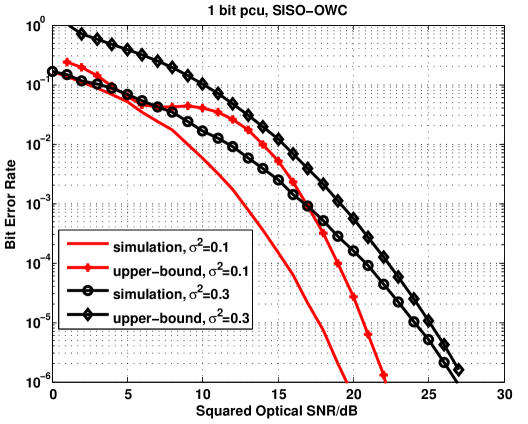
Figure 1: Error performance of SISO-OWC

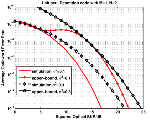
Figure 2: Error performance of MIMO-OWC

In the following, we simulate to verify our newly developed criterion in (III-C). In light of our work being initiative, the only space-only transmission scheme available in the literature is spatial multiplexing. Accordingly, we compare the performance of spatial multiplexing and FDSC specifically designed for $2\times 2$ MIMO-OWC in Section IV. In addition, we suppose that $h_{ij},i,j=1,2$ are independently and identically distributed and let $\sigma_{11}=\sigma_{12}=\sigma_{21}=\sigma_{22}=\sigma$. These schemes are as follows:

1. FDSC. The optical power is normalized in such a way that $\sum_{i,j=1}^{2}f_{ij}=2$ yields $E\left[\sum_{i,j=1}^{2}f_{ij}s_{j}\right]=1$. From (16), the coding matrix is $\mathbf{F}_{FDSC}=\frac{1}{3}\left({\begin{array}[]{cc}2&1\\ 2&1\\ \end{array}}\right)$.

2. Spatial Multiplexing. We fix the modulation formats to be OOK and vary $\sigma^{2}$. So the rate is 2 bits per channel use (pcu). The transmitted symbols $s_{1},s_{2}$ are chosen from $\{0,1\}$ equally likely. The average optical power is $E\left[s_{1}+s_{2}\right]=1$.

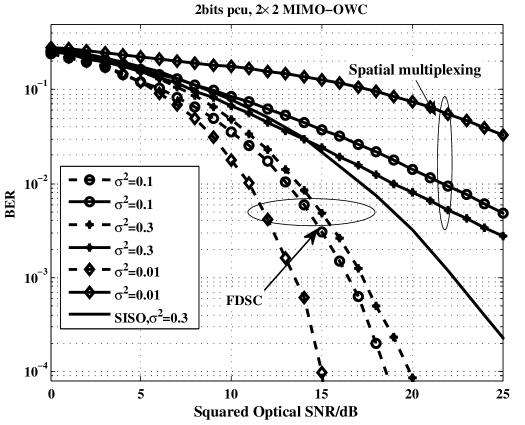
Figure 3: BER comparisons of FDSC and spatial multiplexing.

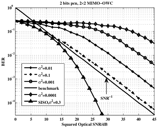
Figure 4: BER comparisons of spatial multiplexing.

We can see that both schemes have the same spectrum efficiency, i.e., 2 bits pcu and the same optical power. Through numerical results, we have following observations.

1. Substantial enhancement from FDSC is achieved, as shown in Fig. 3. For $\sigma^{2}=0.01$, the improvement is almost 16 dB at the target bit error rate (BER) of $10^{-2}$. For $\sigma^{2}=0.5$, the improvement is almost 6 dB at the target BER of $10^{-3}$. Note that the small-scale gain also governs the negative slope of error curve. The decaying speed of the error curve of FDSC is exponential in terms of $\ln\frac{\rho}{\ln^{2}\rho}$ and that of spatial multiplexing is power-law with respect to $\rho$. The reason for this difference is that FDSCs are full-diversity guaranteed by the positive constraints in (IV-A), whereas spatial multiplexing does not satisfy the positive requirement in Theorem 2.

2. Spatial multiplexing presents only small-scale diversity gain illustrated in Fig. 4. By varying the variance of $\mathbf{H}$, we find that in the high SNR regimes, the error curve decays as $\rho^{-1}$ as long as the SNR is high enough. From $\sigma^{2}=0.001$ to $\sigma^{2}=0.1$, the error curve has a horizonal shift, which is the typical style of MIMO RF [24]. The reason is given as follows. The equivalent space coding matrix is $\mathbf{e}^{T}\mathbf{e}=\left({\begin{array}[]{cc}e_{1}^{2}&e_{1}e_{2}\\ e_{1}e_{2}&e_{2}^{2}\\ \end{array}}\right),e_{1},e_{2}\in\{0,\pm 1\}$ with $e_{1}^{2}+e_{2}^{2}\neq 0$. It should be noted that there exists two typical error events: $e_{1}e_{2}=-1$ and $e_{1}e_{2}=0$. From the necessity proof of Theorem 2, for $e_{1}e_{2}=-1$, the attained large-scale diversity gain is zero, and at the same time, if $e_{1}e_{2}=0$ with $e_{1}^{2}+e_{2}^{2}\neq 0$, then, the attained large-scale diversity gain is only two for $2\times 2$ MIMO-OWC. Therefore, the overall large-scale diversity gain of spatial multiplexing is zero with small-scale diversity gain being attained.

3. From Fig. 3 and 4, we notice that when $\sigma$ increases, the error performances of repetition codes will worsen. For this phenomenon, the reason is that for repetition codes, the large-scale diversity is given by $\Omega=\sum_{i,j=1}^{2}\sigma_{ij}^{-2}$, which dominates the exponential decaying speed. However, for spatial multiplexing, increasing $\sigma^{2}$ will improves the error performance by providing a horizontal shift to the left. It is known that since an exact error probability formula for OWC over log-normal fading channels is indeed hard to be obtained particularly for MIMO-OWC, it is very challenging to theoretically prove that the relationship between the error performance of spatial multiplexing and $\sigma^{2}$. Intuitively speaking, the relationship between the error performance of spatial multiplexing and $\sigma^{2}$ follows the radio frequency MIMO. That is to say, $\sigma^{2}$ is the average electrical power of $\ln h$. That’s why increasing $\sigma^{2}$ will improve the error performance of spatial multiplexing, as shown by Figs. 3 and 4.

We can see that the performance gain of MIMO-OWC if any will become larger against increasing SNR in a high enough regime. This implies that a slight improvement in the coding structure will result in a significant enhancement of error performance in the high SNR regimes instead of only an horizonal shift to the left. Unique characteristics of MIMO-OWC are experimentally uncovered and our established criterion are verified.

VI Conclusion and Discussions

In this paper, we have established a general criterion on the full-diversity space coded transmission of MIMO-OWC for the ML receiver, which is, to our best knowledge, the first design criterion for the full-diversity transmission of optical wireless communications with IM/DD over log-normal fading channels. Particularly for a $2\times 2$ case, we have attained a closed-form solution to the optimal linear FDSC design problem, proving that RC is the optimal among all the linear space codes. Our results indicate that the transmission design is indeed necessary and essential for significantly improving overall error performance for MIMO-OWC. However, the design criterion and the specific code constructions for MIMO-OWC presented in this paper are just initiative. Some significant issues are under consideration:

1. Our proposed criterion can be applicable to any non-linear designs. It remains open whether there exists any better non-linear space code than RC.

2. It has been shown in this paper that the space dimension alone is sufficient for full large-scale diversity. Here, a natural question is: what kind of benefit can be obtained if space-time block code designs are used for MIMO-OWC?

3. Like MIMO techniques for RF communications, what is the diversity-multiplexing tradeoff for MIMO-OWC?

-A Proof of Lemma 1

Our main idea here is to split the whole integral in (5) into two parts by properly choosing $\tau>0$ such that its dominant term can be extracted. In other words, the average SEP [43] can be rewritten by

$$P_{e}\left(\rho\right) = \int_{0}^{\tau}Q\left(\frac{\sqrt{\rho}h}{P_{op}}\right)f_{H}\left(h\right)dh$$ (17)

$$+ \int_{\tau}^{\infty}Q\left(\frac{\sqrt{\rho}h}{P_{op}}\right)f_{H}\left(h\right)dh.$$

Now, we select $\tau$ to satisfy that when $\rho\rightarrow\infty$, $\tau\rightarrow 0$, to fragment $\left(0,\infty\right)$ into $\left(0,\tau\right)$ and $\left(\tau,\infty\right)$, adaptively with SNR. This fragmentation is to find the dominant term of $P_{e}\left(\rho\right)$ in the high SNR regimes by giving the upper-bound and the lower bound of $\int_{0}^{\tau}Q\left(\frac{\sqrt{\rho}h}{P_{op}}\right)f_{H}\left(h\right)dh$, and the upper-bounds of $\int_{\tau}^{\infty}Q\left(\frac{\sqrt{\rho}h}{P_{op}}\right)f_{H}\left(h\right)dh$ and then, examining their asymptotical behaviors related with $\tau$. Temporarily, we take this fragmentation for granted and then, will explain the essential reason later on.

-A1 Upper-bound of SEP over $\left(0,\tau\right)$

We integrate the first part of SEP in (17), which is denoted by ${P}_{\tau}\left(\rho\right)$. Notice that when $\rho\rightarrow\infty$, $\tau\rightarrow 0$, and in this case, $f_{H}\left(h\right)$ is monotonically increasing over $\left(0,\tau\right)$. Hence, ${P}_{\tau}\left(\rho\right)$ is upper-bounded by

$${P}_{\tau}\left(\rho\right) \leq f_{H}\left(\tau\right)\int_{0}^{\tau}Q\left(\frac{\sqrt{\rho}h}{P_{op}}\right)dh$$ (18)

$$\leq \frac{f_{H}\left(\tau\right)}{2}\int_{0}^{\tau}\exp\left(-\frac{\rho h^{2}}{2P_{op}^{2}}\right)dh$$

where the last inequality is obtained by using the Chernoff bound on the Gaussian tail integral. Furthermore, we can upper-bound the last integral of (18) by

$$\int_{0}^{\tau}\exp\left(-\frac{\rho h^{2}}{2P_{op}^{2}}\right)dh = P_{op}\sqrt{2\pi}\rho^{-\frac{1}{2}}\left(\frac{1}{2}-Q\left(\frac{\sqrt{{\rho\tau^{2}}}}{P_{op}}\right)\right)$$ (19)

$$\leq \frac{P_{op}\sqrt{2\pi}}{2}\rho^{-\frac{1}{2}}$$

which produces

$${P}_{\tau}\left(\rho\right) \leq \frac{P_{op}\sqrt{2\pi}f_{H}\left(\tau\right)}{4}\rho^{-\frac{1}{2}}$$ (20)

$$= \frac{P_{op}\exp\left(\frac{\sigma^{2}}{2}\right)}{4\sqrt{\sigma^{2}}}\rho^{-\frac{1}{2}}\exp\left(-\frac{\left(\ln\tau+\sigma^{2}\right)^{2}}{2\sigma^{2}}\right)$$

-A2 Lower-bound of SEP

At the same time, when $\rho\rightarrow\infty$, we have $\frac{\tau}{\ln\rho}\leq\tau$. This inequality allows us to lower-bound ${P}_{\tau}\left(\rho\right)$ by

$${P}_{\tau}\left(\rho\right) = \int_{0}^{\tau}Q\left(\frac{\sqrt{\rho}h}{P_{op}}\right)f_{H}\left(h\right)dh$$ (21)

$$\geq \int_{0}^{\frac{\tau}{\ln\rho}}Q\left(\frac{\sqrt{\rho}h}{P_{op}}\right)f_{H}\left(h\right)dh$$

$$\geq \int_{0}^{\frac{\tau}{\ln\rho}}Q\left(\frac{\sqrt{\rho}\tau}{P_{op}\ln\rho}\right)f_{H}\left(h\right)dh$$

where the last inequality follows from the monotonically decreasing property of $Q$-function.

Then, by integrating $f_{H}\left(h\right)$ over $\left(0,\frac{\tau}{\ln\rho}\right)$, we have

$${P}_{\tau}\left(\rho\right)\geq Q\left(\frac{\sqrt{\rho}\tau}{P_{op}\ln\rho}\right)Q\left(\frac{-\ln\tau+\ln\ln\rho}{\sigma}\right)$$ (22)

$$\geq\frac{Q\left(\frac{\sqrt{\rho}\tau}{P_{op}\ln\rho}\right)}{2\sqrt{2\pi}}\frac{\sigma}{\ln\frac{\ln\rho}{\tau}}\exp\left(-\frac{\left(\ln\frac{\tau}{\ln\rho}\right)^{2}}{2\sigma^{2}}\right)$$

where the last inequality is obtained by using

$$Q\left(x\right)\geq\frac{1}{2\sqrt{2\pi}x}\exp\left(-\frac{x^{2}}{2}\right),x\geq\frac{\sqrt{2}}{2}.$$ (23)

-A3 Upper-bound of SEP over $\left(\tau,\infty\right)$

We now turn to the second part of $P_{e}\left(\rho\right)$ in (17), which is denoted by $\bar{P}_{\tau}\left(\rho\right)$. Letting $f^{\prime}_{H}\left(h\right)=0$ produces the point $h_{0}$ satisfying $\forall h\geq 0,f_{H}\left(h\right)\leq f_{H}\left(h_{0}\right)=\frac{\exp\left(\frac{\sigma^{2}}{2}\right)}{\sqrt{2\pi\sigma^{2}}}$. With this, $\bar{P}_{\tau}\left(\rho\right)$ can be upper-bounded by

$$\bar{P}_{\tau}\left(\rho\right) \leq f_{H}\left(h_{0}\right)\int_{\tau}^{\infty}Q\left(\frac{\sqrt{\rho}h}{P_{op}}\right)dh$$

Using Chernoff bound on the Gaussian tail integral gives us

$$\bar{P}_{\tau}\left(\rho\right) \leq \frac{1}{2}f_{H}\left(h_{0}\right)\int_{\tau}^{\infty}\exp\left(-\frac{\rho h^{2}}{2P_{op}^{2}}\right)dh$$ (24)

$$= \frac{1}{2}f_{H}\left(h_{0}\right)\sqrt{2\pi}\rho^{-1/2}Q\left(\frac{\sqrt{{\rho\tau^{2}}}}{P_{op}}\right)$$

$$\leq \frac{\exp\left(\frac{\sigma^{2}}{2}\right)}{4\sqrt{\sigma^{2}}}\rho^{-1/2}\exp\left(-\frac{\rho\tau^{2}}{2P_{op}^{2}}\right)$$

-A4 Determination of $\tau$

Thus far, we have attained three bounds, respectively shown in (20), (22) and (24). Now, we examine their tightness related to $\tau$. We can see that  (20) and (22) have the same exponential term $\frac{\left(\ln\tau\right)^{2}}{\sigma^{2}}$. To make the upper bounds in (20) to approach the upper-bound in (24) as tightly as possible, we seek to select such $\tau$ that

$$\frac{\rho\tau^{2}}{2P_{op}^{2}}=\frac{\left(\ln\tau+\sigma^{2}\right)^{2}}{2\sigma^{2}}$$ (25)

An explicit solution to (25) with respect to $\tau$ is difficult to obtain. Accordingly, we propose to approximate the solution to (25) by

$$\tau=\frac{P_{op}\ln\rho}{2\sqrt{\rho\sigma^{2}}}$$ (26)

which satisfies the following asymptotical equality.

$$\lim_{\rho\rightarrow\infty}\frac{\frac{\rho\tau^{2}}{2P_{op}^{2}}}{\frac{\left(\ln\tau+\sigma^{2}\right)^{2}}{2\sigma^{2}}}=\lim_{\rho\rightarrow\infty}\frac{\left(\ln\rho\right)^{2}}{\left(\ln\frac{\rho}{\ln^{2}\rho}-\ln\frac{P^{2}_{op}}{4\sigma^{2}}\right)^{2}}=1$$

Finally, combining (20), (22), (24), and (26) leads to the fact that there exist three positive constants $C_{1L}$, $C_{11U}$ and $C_{12U}$ independent of $\rho$ such that

$$C_{1L}\frac{1}{\ln\rho-\ln\frac{4\sigma^{2}}{P_{op}^{2}}}\exp\left(-\frac{\left(\ln\rho-\ln\frac{P_{op}^{2}}{4\sigma^{2}}\right)^{2}}{8\sigma^{2}}\right)\leq P_{e}(\rho)$$

$$\leq\frac{1}{4}\left(\ln\rho\right)^{-1}\exp\left(-\frac{\left(\ln\frac{\rho}{\ln^{2}\rho}-\ln\frac{P^{2}_{op}}{4\sigma^{2}}\right)^{2}}{8\sigma^{2}}\right)$$

$$+C_{12U}\rho^{-\frac{1}{2}}\exp\left(-\frac{\left(\ln\rho\right)^{2}}{8\sigma^{2}}\right)$$ (27)

where $C_{1L}=\frac{Q\left(\frac{1}{2\sigma}\right)}{\sqrt{2\pi}}$, $C_{11U}=\frac{1}{2}$ and $C_{12U}=\frac{\exp\left(\frac{\sigma^{2}}{2}\right)}{4\sqrt{\sigma^{2}}}$. This is the complete proof of Lemma 1.  $\Box$

-B Proof of Theorem 1

The condition that any $\mathbf{e}\in{\mathcal{E}}$ is unipolar without zero entry implies that if $\forall\tau>0$ and $\forall\mathbf{e}\in{\mathcal{E}}$, $\left(\mathbf{e}^{T}\mathbf{h}_{i}\right)^{2}\leq\tau^{2}$, then, we can have $h_{ij}\leq\frac{\tau}{|e_{j}|},i=1,\ldots,M,j=1,\ldots,N$. After these preparations, we adopt the same techniques as Subsection III-A. Temporally, assume that when $\rho\rightarrow\infty$, $\tau\rightarrow 0$. Similarly, $P\left(\mathbf{s}\rightarrow\hat{\mathbf{s}}\right)$ can be adaptively fragmented with SNR as

$$P\left(\mathbf{s}\rightarrow\hat{\mathbf{s}}\right)=\int_{\left(\mathbf{e}^{T}\mathbf{h}_{j}\right)^{2}\leq\tau^{2}}P\left(\mathbf{s}\rightarrow\hat{\mathbf{s}}|\mathbf{H}\right)f_{\mathbf{H}}\left(\mathbf{H}\right)d\mathbf{H}+\int_{\left(\mathbf{e}^{T}\mathbf{h}_{j}\right)^{2}>\tau^{2}}P\left(\mathbf{s}\rightarrow\hat{\mathbf{s}}|\mathbf{H}\right)f_{\mathbf{H}}\left(\mathbf{H}\right)d\mathbf{H}.$$ (28)

The target in the ensuing subsections is to give the asymptotical bounds on $P\left(\mathbf{s}\rightarrow\hat{\mathbf{s}}\right)$ following the similar procedures to the case of SISO-OWC.

-B1 Upper-bound of PEP over $\left(0,\tau\right)$

To begin with, let us process the first part of $P\left(\mathbf{s}\rightarrow\hat{\mathbf{s}}\right)$ in (28) denoted by $P_{\tau}\left(\mathbf{s}\rightarrow\hat{\mathbf{s}}\right)$. We know when $\rho\rightarrow\infty$, $\tau\rightarrow 0$. In this instance, $f_{H}\left(h_{ij}\right)$ is monotonically increasing over $\left(0,\frac{\tau}{|e_{i}|}\right)$ and then, $f_{H}\left(h_{ij}\right)\leq f_{H}\left(\frac{\tau}{|e_{j}|}\right)$. Together with the Chernoff bound of $Q$-function, $P_{\tau}\left(\mathbf{s}\rightarrow\hat{\mathbf{s}}\right)$ can be upper-bounded by

$$P_{\tau}\left(\mathbf{s}\rightarrow\hat{\mathbf{s}}\right)\leq\frac{1}{2}\prod_{j=1}^{N}\prod_{i=1}^{M}f_{H_{ij}}\left(\frac{\tau}{|e_{j}|}\right)\int_{\left(\mathbf{e}^{T}\mathbf{h}_{i}\right)^{2}\leq\tau^{2}}\exp\left(-\frac{\rho\sum_{i=1}^{M}\left(\mathbf{e}^{T}\mathbf{h}_{i}\right)^{2}}{8NP_{op}^{2}}\right)d\mathbf{H}$$ (29a)

In addition, by Assumption 1, $$e_{1},~{}\cdots,~{}e_{N} P_{\tau}\left(\mathbf{s}\rightarrow\hat{\mathbf{s}}\right)$$ have the same signs. This result allows us to further upper-bound by

$$P_{\tau}\left(\mathbf{s}\rightarrow\hat{\mathbf{s}}\right)\leq\frac{1}{2}\prod_{j=1}^{N}\prod_{i=1}^{M}f_{H_{ij}}\left(\frac{\tau}{|e_{j}|}\right)\times\int_{h_{ij}\leq\frac{\tau}{|e_{j}|}}\exp\left(-\frac{\rho\sum_{j=1}^{N}\sum_{i=1}^{M}e_{j}^{2}h_{ij}^{2}}{8NP_{op}^{2}}\right)d\mathbf{H}$$ (29b)

Further, integrating the last term in (29b) produces

$$P_{\tau}\left(\mathbf{s}\rightarrow\hat{\mathbf{s}}\right)\leq\frac{1}{2}\prod_{j=1}^{N}\prod_{i=1}^{M}f_{H_{ij}}\left(\frac{\tau}{|e_{j}|}\right)\prod_{j=1}^{N}\prod_{i=1}^{M}\sqrt{2\pi}\left(\frac{\rho|e_{j}|^{2}}{4NP_{op}^{2}}\right)^{-\frac{1}{2}}\left(\frac{1}{2}-Q\left(\frac{\rho\tau^{2}}{4NP_{op}^{2}}\right)\right)$$

$$\leq\frac{1}{2}\prod_{j=1}^{N}\prod_{i=1}^{M}\frac{\sqrt{2\pi}}{2}f_{H_{ij}}\left(\frac{\tau}{|e_{j}|}\right)\left(\frac{\rho|e_{j}|^{2}}{4NP_{op}^{2}}\right)^{-\frac{1}{2}}$$

$$=\frac{\tau^{-MN}}{2\prod_{j=1}^{N}\prod_{i=1}^{M}\sqrt{\sigma_{ij}^{2}}}\left(\frac{\rho}{NP_{op}^{2}}\right)^{-\frac{MN}{2}}\exp\left(-\sum_{j=1}^{N}\sum_{i=1}^{M}\frac{\left(\ln\tau-\ln|e_{j}|\right)^{2}}{2\sigma_{ij}^{2}}\right)$$ (29c)

-B2 Lower-bound of PEP over $\left(0,\tau\right)$

To attain the lower bound of $P_{\tau}\left(\mathbf{s}\rightarrow\hat{\mathbf{s}}\right)$, we need the following preparations. We observe that $\mathbf{e}\mathbf{e}^{T}$ is rank-one with the only non-zero eigenvalue being $\lambda_{\max}=\sum_{j=1}^{N}e_{j}^{2}$. Then, $\mathbf{h}_{i}^{T}\mathbf{e}\mathbf{e}^{T}\mathbf{h}_{i}\leq\lambda_{\max}\sum_{j=1}^{N}h_{ij}^{2},i=1,\ldots,M$. In other words, for all $\tau>0$, it holds that

$$\{\mathbf{H}:\mathbf{h}_{i}\in\mathbb{R}^{N}_{+},\lambda_{\max}\sum_{j=1}^{N}h_{ij}^{2}\leq\tau^{2},i=1,\ldots,M\}$$

$$\subseteq\{\mathbf{H}:\mathbf{h}_{i}\in\mathbb{R}^{N}_{+},\mathbf{h}_{i}^{T}\mathbf{e}\mathbf{e}^{T}\mathbf{h}_{i}\leq\tau^{2},i=1,\ldots,M\}$$ (30a)

Further, it is true that

$$\{\mathbf{H}:0\leq h_{ij}\leq\frac{\tau}{\sqrt{N\lambda_{\max}}},j=1,\ldots,N,i=1,\ldots,M\}$$ (30b)

$$\subseteq\{\mathbf{H}:\lambda_{\max}\sum_{j=1}^{N}h_{ij}^{2}\leq\tau^{2},i=1,\ldots,M\}$$

$$\subseteq\{\mathbf{H}:\mathbf{h}_{i}\in\mathbb{R}^{N}_{+},\mathbf{h}_{i}^{T}\mathbf{e}\mathbf{e}^{T}\mathbf{h}_{i}\leq\tau^{2},i=1,\ldots,M\}$$

Now, by (30b), we can lower-bound $P_{\tau}\left(\mathbf{s}\rightarrow\hat{\mathbf{s}}\right)$ by

$$P_{\tau}\left(\mathbf{s}\rightarrow\hat{\mathbf{s}}\right)\geq\int_{h_{ij}\leq\frac{\tau}{\sqrt{N\sum_{k=1}^{N}e_{k}^{2}}}}P\left(\mathbf{s}\rightarrow\hat{\mathbf{s}}|\mathbf{H}\right)f_{\mathbf{H}}\left(\mathbf{H}\right)d\mathbf{H}$$

$$\geq Q\left(\frac{\sqrt{M\rho}\tau}{2NP_{op}\sqrt{\sum_{k=1}^{N}e_{k}^{2}}}\right)\int_{h_{ij}\leq\frac{\tau}{\sqrt{N\sum_{k=1}^{N}e_{k}^{2}}}}f_{\mathbf{H}}\left(\mathbf{H}\right)d\mathbf{H}$$

$$\geq Q\left(\frac{\sqrt{M\rho}\tau}{2NP_{op}\ln\rho\sqrt{\sum_{k=1}^{N}e_{k}^{2}}}\right)\prod_{j=1}^{N}\prod_{i=1}^{M}Q\left(-\frac{\ln\frac{\tau}{\ln\rho\sqrt{N\sum_{k=1}^{N}e_{k}^{2}}}}{\sigma_{ij}^{2}}\right)$$ (31a)

where the last inequality holds for high SNR such that $$\ln\rho>1$$. Again, by (23), we arrive at the following lower-bound by

$$P_{\tau}\left(\mathbf{s}\rightarrow\hat{\mathbf{s}}\right)\geq\frac{\exp\left(\frac{MN}{2}\right)}{\left(4\pi\right)^{MN}}Q\left(\frac{\sqrt{M\rho}\tau}{2NP_{op}\ln\rho\sqrt{\sum_{k=1}^{N}e_{k}^{2}}}\right)$$ (31b)

$$\times\frac{\prod_{j=1}^{N}\prod_{i=1}^{M}\sigma_{ij}}{\ln^{MN}\frac{\ln\rho\sqrt{N\sum_{k=1}^{N}e_{k}^{2}}}{\tau}}\exp\left(-\sum_{j=1}^{N}\sum_{i=1}^{M}\frac{1}{2\sigma_{ij}^{2}}\left(\ln\frac{\tau}{\ln\rho\sqrt{N\sum_{k=1}^{N}e_{k}^{2}}}\right)^{2}\right)$$

-B3 Upper-bound of PEP over $\left(\tau,\infty\right)$

Now, we are in a position to analyze $P\left(\mathbf{s}\rightarrow\hat{\mathbf{s}}\right)-P_{\tau}\left(\mathbf{s}\rightarrow\hat{\mathbf{s}}\right)$, i.e., the second term of (28), which is denoted by $\bar{P}_{\tau}\left(\mathbf{s}\rightarrow\hat{\mathbf{s}}\right)$.

Similarly, for $h_{ij}$, $f^{\prime}_{H}\left(h_{ij}\right)=0$ gives the extreme point $h_{ij,0}$ of $f_{H}\left(h_{ij}\right)$, i.e., $f_{H}\left(h_{ij}\right)\leq f_{H}\left(h_{ij,0}\right),i=1,\ldots,M,j=1,\ldots,N$ . Then, we have $f_{\mathbf{H}}\left(\mathbf{H}\right)\leq f_{\mathbf{H}}\left(\mathbf{H}_{0}\right)$ and thus, $\bar{P}_{\tau}\left(\mathbf{s}\rightarrow\hat{\mathbf{s}}\right)$ can be upper-bounded by

$$\bar{P}_{\tau}\left(\mathbf{s}\rightarrow\hat{\mathbf{s}}\right)\leq\frac{f_{\mathbf{H}}\left(\mathbf{H}_{0}\right)}{2}\int_{\left(\mathbf{e}^{T}\mathbf{h}_{i}\right)^{2}>\tau^{2}}\exp\left(-\frac{\rho\sum_{i=1}^{M}\mathbf{h}_{i}^{T}\mathbf{e}\mathbf{e}^{T}\mathbf{h}_{i}}{8NP_{op}^{2}}\right)d\mathbf{H}$$ (32a)

In fact, (30b) also implies $\{\mathbf{H}:\mathbf{h}_{i}^{T}\mathbf{e}\mathbf{e}^{T}\mathbf{h}_{i}\geq\tau^{2},i=1,\ldots,M\}\subseteq\{\mathbf{H}:h_{ij}\geq\frac{\tau}{\sqrt{N\sum_{k=1}^{N}e_{k}^{2}}},i=1,\ldots,M,j=1,\ldots,N\}$. With this, $\bar{P}_{\tau}\left(\mathbf{s}\rightarrow\hat{\mathbf{s}}\right)$ can be further upper-bounded by

$$\bar{P}_{\tau}\left(\mathbf{s}\rightarrow\hat{\mathbf{s}}\right)\leq\frac{f_{\mathbf{H}}\left(\mathbf{H}_{0}\right)}{2}\int_{h_{ij}\geq\frac{\tau}{\sqrt{N\sum_{k=1}^{N}e_{k}^{2}}}}\exp\left(-\frac{\rho\lambda_{\max}\sum_{i=1}^{M}\sum_{j=1}^{N}h_{ij}^{2}}{8NP_{op}^{2}}\right)d\mathbf{H}$$

$$=\frac{f_{\mathbf{H}}\left(\mathbf{H}_{0}\right)}{2}\prod_{i=1}^{M}\prod_{j=1}^{M}\sqrt{2\pi}\left(\frac{\rho\sum_{k=1}^{N}e_{k}^{2}}{4NP_{op}^{2}}\right)^{-\frac{1}{2}}Q\left(\sqrt{\frac{\rho\tau^{2}}{4N^{2}P_{op}^{2}}}\right)$$

$$\leq\frac{\exp\left(\frac{\sum_{i=1}^{M}\sum_{j=1}^{N}\sigma_{ij}^{2}}{2}\right)}{2\prod_{i=1}^{M}\prod_{j=1}^{N}\sigma_{ij}}\left(\frac{\rho\sum_{k=1}^{N}e_{k}^{2}}{NP_{op}^{2}}\right)^{-\frac{MN}{2}}\exp\left(-\frac{M\rho\tau^{2}}{8NP_{op}^{2}}\right)$$ (32b)

So far, we have attained three bounds and now, examine their tightness to select $\tau$ in the following subsection.

-B4 Selection of $\tau$

It is noticed that the exponential terms of (29) and (31b) are the same, i.e., $\left(\ln\tau\right)^{2}\sum_{i=1}^{M}\sum_{j=1}^{N}\sigma_{ij}^{-2}$. To mathch the bounds (29) and (-B3), $\tau$ is selected such that

$$\frac{M\rho\tau^{2}}{8NP_{op}^{2}}=\left(\ln\tau\right)^{2}\sum_{i=1}^{M}\sum_{j=1}^{N}\frac{\sigma_{ij}^{-2}}{2}$$ (33)

Since a closed-form solution to (33) is hard to attain. the solution to (33) is approximated below

$$\tau=\sqrt{\frac{NP_{op}^{2}}{M}\sum_{i=1}^{M}\sum_{j=1}^{N}\sigma_{ij}^{-2}}\frac{\ln\rho}{\sqrt{\rho}}$$ (34)

For the selection in (34), the following asymptotical equality holds.

$$\lim_{\rho\rightarrow\infty}\frac{\frac{M\rho\tau^{2}}{8NP_{op}^{2}}}{\left(\ln\tau\right)^{2}\sum_{i=1}^{M}\sum_{j=1}^{N}\frac{\sigma_{ij}^{-2}}{2}}$$

$$=\lim_{\rho\rightarrow\infty}\frac{\left(\ln\rho\right)^{2}}{\left(\ln\frac{\rho}{\ln^{2}\rho}-\ln\left(\frac{NP_{op}^{2}}{M}\sum_{i=1}^{M}\sum_{j=1}^{N}\sigma_{ij}^{-2}\right)\right)^{2}}$$

$$=1$$

Then, putting (29), (31b), (-B3) and (34) together, we are allowed to arrive at the fact that there exists three positive constants $C_{2L}$, $C_{2U}$ and $C_{3U}$, independent of $\rho$ shown by (-B4), postponed to the top of the next page,

$$\underbrace{C_{2L}\left(\ln\rho\right)^{-MN}e^{-\sum_{i=1}^{M}\sum_{j=1}^{N}\frac{\left(\ln\rho+\ln\left(P_{op}^{2}\Omega\right)-\ln\left(M\sum_{k=1}^{N}e_{k}^{2}\right)\right)^{2}}{8\sigma_{ij}^{2}}}}_{P_{L}\left(\mathbf{s}\rightarrow\hat{\mathbf{s}}\right)}\leq P\left(\mathbf{s}\rightarrow\hat{\mathbf{s}}\right)$$

$$\leq\underbrace{C_{2U}\left(\ln\rho\right)^{-MN}e^{-\sum_{i=1}^{M}\sum_{j=1}^{N}\frac{\left(\ln\frac{\rho}{\ln^{2}\rho}+\ln\left(P_{op}^{2}\Omega\right)-\ln e_{j}^{2}\right)^{2}}{8\sigma_{ij}^{2}}}}_{P_{U1}\left(\mathbf{s}\rightarrow\hat{\mathbf{s}}\right)}+\underbrace{C_{3U}\rho^{-\frac{MN}{2}}e^{-\sum_{i=1}^{M}\sum_{j=1}^{N}\frac{\ln^{2}\rho}{8\sigma_{ij}^{2}}}}_{P_{U2}\left(\mathbf{s}\rightarrow\hat{\mathbf{s}}\right)}$$ (35)

 

where

$$\Omega=\sum_{i=1}^{M}\sum_{j=1}^{N}\sigma_{ij}^{-2}$$ (36a)

$$C_{2L}=\frac{\prod_{i=1}^{M}\prod_{j=1}^{N}\sigma_{ij}}{\left(4\pi\right)^{MN}\exp\left(-\frac{MN}{2}\right)}Q\left(\frac{1}{2}\left(\sum_{k=1}^{N}e_{k}^{2}\right)^{-\frac{1}{2}}\right)$$ (36b)

$$C_{2U}=\frac{\left(NP_{op}^{2}\right)^{MN}}{2\prod_{i=1}^{M}\prod_{j=1}^{N}\sqrt{\sigma_{ij}^{2}}}\exp\left(-\frac{\Omega}{8}\ln^{2}\left(\frac{NP_{op}^{2}\Omega}{M}\right)\right)$$ (36c)

$$C_{3U}=\frac{\exp\left(\frac{\sum_{i=1}^{M}\sum_{j=1}^{N}\sigma_{ij}^{2}}{2}\right)}{2\prod_{i=1}^{N}\prod_{j=1}^{M}\sigma_{ij}}\left(\frac{\sum_{k=1}^{N}e_{k}^{2}}{NP_{op}^{2}}\right)^{-\frac{MN}{2}}$$ (36d)

Now, we can see that in (-B4), $P_{L}\left(\mathbf{s}\rightarrow\hat{\mathbf{s}}\right)$ and $P_{U2}\left(\mathbf{s}\rightarrow\hat{\mathbf{s}}\right)$ have the same exponential term, $\exp\left(-\frac{\Omega}{8}\ln^{2}\rho\right)$, whereas the exponential term of $P_{U1}\left(\mathbf{s}\rightarrow\hat{\mathbf{s}}\right)$ is $\exp\left(-\frac{\Omega}{8}\ln^{2}\frac{\rho}{\ln^{2}\rho}\right)$, which decays slower than $\exp\left(-\frac{\Omega}{8}\ln^{2}\rho\right)$ against high SNRs. That being said, we have attained the dominant term, $P_{U1}\left(\mathbf{s}\rightarrow\hat{\mathbf{s}}\right)$, of the upper-bound of $P\left(\mathbf{s}\rightarrow\hat{\mathbf{s}}\right)$. This completes the proof of Theorem 1.  $\Box$

-C Proof of Property 1

For $m_{1}\perp n_{1}$, $m_{2}\perp n_{2}$ and $m_{3}\perp n_{3}$, we have that

$$\frac{n_{1}+n_{3}}{m_{1}+m_{3}}\geq\frac{n_{2}}{m_{2}}\Leftrightarrow m_{2}n_{3}-m_{3}n_{2}\geq m_{1}n_{2}-m_{2}n_{1}$$

This is indeed true, since we obtain $m_{1}n_{2}-m_{2}n_{1}=1$ by Lemma 1 and $m_{2}n_{3}-m_{3}n_{2}\geq 1$ from the assumption that $\frac{n_{2}}{m_{2}}<\frac{n_{3}}{m_{3}}$.

In the same token, given $m_{0}\perp n_{0}$, $m_{1}\perp n_{1}$ and $m_{2}\perp n_{2}$, we have that

$$\frac{n_{0}+n_{2}}{m_{0}+m_{2}}\leq\frac{n_{1}}{m_{1}}\Leftrightarrow m_{0}n_{1}-m_{1}n_{0}\geq m_{1}n_{2}-m_{2}n_{1}$$

This indeed holds, since we can attain $m_{1}n_{2}-m_{2}n_{1}=1$ by Lemma 1 and $m_{0}n_{1}-m_{1}n_{0}\geq 1$ from the assumption that $\frac{n_{0}}{m_{0}}<\frac{n_{1}}{m_{1}}$. This completes the proof of Property 1.   $\Box$

-D Proof of Property 2

First, Statement 1: $\frac{n_{1}}{m_{1}}<\frac{n_{1}+n_{2}}{m_{1}+m_{2}}<\frac{n_{2}}{m_{2}}$ can be verified by

$$\frac{n_{1}+n_{2}}{m_{1}+m_{2}}-\frac{n_{2}}{m_{2}}=\frac{m_{1}}{\left(m_{1}+m_{2}\right)}\left(\frac{n_{1}}{m_{1}}-\frac{n_{2}}{m_{2}}\right)<0,$$

$$\frac{n_{1}+n_{2}}{m_{1}+m_{2}}-\frac{n_{1}}{m_{1}}=\frac{m_{2}}{\left(m_{1}+m_{2}\right)}\left(\frac{n_{2}}{m_{2}}-\frac{n_{1}}{m_{1}}\right)>0.$$

When $\frac{f_{11}}{f_{12}},\frac{f_{21}}{f_{22}}\in\left(\frac{n_{1}}{m_{1}},\frac{n_{2}}{m_{2}}\right)$, we can have $\left(m_{1}f_{11}-n_{1}f_{12}\right)>0$ and $\left(m_{2}f_{11}-n_{2}f_{12}\right)<0$. Hence,

$$|m_{1}f_{11}-n_{1}f_{12}|-|m_{2}f_{11}-n_{2}f_{12}|=\left(m_{1}+m_{2}\right)f_{12}\left(\frac{f_{11}}{f_{12}}-\frac{n_{1}+n_{2}}{m_{1}+m_{2}}\right)$$ (37a)

and

$$|m_{1}f_{21}-n_{1}f_{22}|-|m_{2}f_{21}-n_{2}f_{22}|=\left(m_{1}+m_{2}\right)f_{22}\left(\frac{f_{21}}{f_{22}}-\frac{n_{1}+n_{2}}{m_{1}+m_{2}}\right).$$ (37b)

Combining (37a) and (37b) leads us to the following facts:

1. If $\frac{f_{11}}{f_{12}},\frac{f_{21}}{f_{22}}\in\left(\frac{n_{1}}{m_{1}},\frac{n_{1}+n_{2}}{m_{1}+m_{2}}\right)$, then, we have

   $$-m_{2}f_{11}+n_{2}f_{12}>m_{1}f_{11}-n_{1}f_{12}>0,-m_{2}f_{21}+n_{2}f_{22}>m_{1}f_{21}-n_{1}f_{22}>0$$

   Thus, $F_{m_{1}n_{1}}<F_{m_{2}n_{2}}$ holds.

2. If $\frac{f_{11}}{f_{12}},\frac{f_{21}}{f_{22}}\in\left(\frac{n_{1}+n_{2}}{m_{1}+m_{2}},\frac{n_{2}}{m_{2}}\right)$, then, we arrive at

   $$m_{1}f_{11}-n_{1}f_{12}>-m_{2}f_{11}+n_{2}f_{12}>0$$

   $$m_{1}f_{21}-n_{1}f_{22}>-m_{2}f_{21}+n_{2}f_{22}>0.$$

   Hence, we have $F_{m_{1}n_{1}}>F_{m_{2}n_{2}}$.

3. If $\frac{f_{11}}{f_{12}}=\frac{f_{21}}{f_{22}}=\frac{n_{1}+n_{2}}{m_{1}+m_{2}}$, then $F_{m_{1}n_{1}}=F_{m_{2}n_{2}}$.

This completes the proof of Property 2.   $\Box$

-E proof of Property 3

$\forall\frac{n_{0}}{m_{0}},\frac{n_{3}}{m_{3}}\in\mathfrak{F}_{k}$ satisfying $\frac{n_{0}}{m_{0}}<\frac{n_{1}}{m_{1}}<\frac{n_{2}}{m_{2}}<\frac{n_{3}}{m_{3}}$, when $\frac{f_{11}}{f_{12}},\frac{f_{21}}{f_{22}}\in\left(\frac{n_{1}}{m_{1}},\frac{n_{2}}{m_{2}}\right)$, we have $F_{m_{0}n_{0}},F_{m_{1}n_{1}},F_{m_{2}n_{2}},F_{m_{3}n_{3}}>0$. Property 1 tells us that $\frac{n_{1}+n_{3}}{m_{1}+m_{3}}\geq\frac{n_{2}}{m_{2}}$ and $\frac{n_{0}+n_{2}}{m_{0}+m_{2}}\leq\frac{n_{1}}{m_{1}}$. As a result, we can have

$$\left(\frac{n_{1}}{m_{1}},\frac{n_{2}}{m_{2}}\right)\subseteq\left(\frac{n_{0}+n_{2}}{m_{0}+m_{2}},\frac{n_{2}}{m_{2}}\right)\subseteq\left(\frac{n_{0}}{m_{0}},\frac{n_{2}}{m_{2}}\right)$$

$$\left(\frac{n_{1}}{m_{1}},\frac{n_{2}}{m_{2}}\right)\subseteq\left(\frac{n_{1}}{m_{1}},\frac{n_{1}+n_{3}}{m_{1}+m_{3}}\right)\subseteq\left(\frac{n_{1}}{m_{1}},\frac{n_{3}}{m_{3}}\right)$$

Using Property 2, we can attain $F_{m_{0}n_{0}}>F_{m_{2}n_{2}}$ and $F_{m_{1}n_{1}}<F_{m_{3}n_{3}}$. The successivity of $\frac{n_{1}}{m_{1}}$ and $\frac{n_{2}}{m_{2}}$ ensures $F_{m_{1}n_{1}}$ and $F_{m_{2}n_{2}}$ are the last two minimum over $\left(\frac{n_{1}}{m_{1}},\frac{n_{2}}{m_{2}}\right)$. This completes the proof of Property 3.   $\Box$

-F proof of Theorem 3

Assume $\frac{n_{1}}{m_{1}}$ and $\frac{n_{2}}{m_{2}}$ are varying two successive items of $\mathfrak{F}_{2^{p}-1}$ and denote $x=\frac{f_{11}}{f_{12}}$ and $y=\frac{f_{21}}{f_{22}}$. These notations produce $f_{12}\left(1+x\right)+f_{22}\left(1+y\right)=1$. We firstly prove that if $x,y\in\left(\frac{n_{1}}{m_{1}},\frac{n_{2}}{m_{2}}\right)$, then the local solution to (IV-A) is determined by

$$x = y=\frac{n_{1}+n_{2}}{m_{1}+m_{2}},$$

$$f_{12} = f_{22}=\frac{m_{1}+m_{2}}{2\left(m_{1}+m_{2}+n_{1}+n_{2}\right)}$$ (38)

Letting $\left(xm_{1}-n_{1}\right)\left(ym_{1}-n_{1}\right)\leq\left(xm_{2}-n_{2}\right)\left(ym_{2}-n_{2}\right)$ yields $x\leq\frac{n_{1}\left(ym_{1}-n_{1}\right)-n_{2}\left(ym_{2}-n_{2}\right)}{m_{1}\left(ym_{1}-n_{1}\right)-m_{2}\left(ym_{2}-n_{2}\right)}$. In the same token, $\left(xm_{1}-n_{1}\right)\left(ym_{1}-n_{1}\right)\geq\left(xm_{2}-n_{2}\right)\left(ym_{2}-n_{2}\right)$ implies $y\leq\frac{n_{2}\left(xm_{2}-n_{2}\right)-n_{1}\left(xm_{1}-n_{1}\right)}{m_{2}\left(xm_{2}-n_{2}\right)-m_{1}\left(xm_{1}-n_{1}\right)}$. Then, from Property 2 and Property 3, we have that if $x,y\in\left(\frac{n_{1}}{m_{1}},\frac{n_{2}}{m_{2}}\right)$, then (IV-A) can be equivalent to the following two sub-problems:

1. If $x\leq\frac{n_{1}\left(ym_{1}-n_{1}\right)-n_{2}\left(ym_{2}-n_{2}\right)}{m_{1}\left(ym_{1}-n_{1}\right)-m_{2}\left(ym_{2}-n_{2}\right)}$, then (IV-A) is equivalent to the following problem

   $$\max_{f_{11},f_{12},f_{21},f_{22}}F_{m_{1}n_{1}}$$

   $$s.t.\left\{\begin{array}[]{ll}x\leq\frac{n_{1}\left(ym_{1}-n_{1}\right)-n_{2}\left(ym_{2}-n_{2}\right)}{m_{1}\left(ym_{1}-n_{1}\right)-m_{2}\left(ym_{2}-n_{2}\right)},\\ x,y\in\left(\frac{n_{1}}{m_{1}},\frac{n_{2}}{m_{2}}\right),\\ f_{11}+f_{12}+f_{21}+f_{22}=1.\end{array}\right.$$ (42)

   Over the feasible region of $x$ and with the increasing property of $F_{m_{1}n_{1}}$, we can have

   $$F_{m_{1}n_{1}}\leq\left(m_{1}\frac{n_{1}\left(ym_{1}-n_{1}\right)-n_{2}\left(ym_{2}-n_{2}\right)}{m_{1}\left(ym_{1}-n_{1}\right)-m_{2}\left(ym_{2}-n_{2}\right)}-n_{1}\right)f_{12}f_{22}\left(ym_{1}-n_{1}\right)$$

   $$=\frac{m_{2}y\left(m_{2}n_{1}-m_{1}n_{2}\right)+n_{2}\left(m_{1}n_{2}-m_{2}n_{1}\right)}{{m_{1}\left(ym_{1}-n_{1}\right)-m_{2}\left(ym_{2}-n_{2}\right)}}f_{12}f_{22}\left(ym_{1}-n_{1}\right)$$

   $$=\frac{-f_{12}f_{22}\left(ym_{2}-n_{2}\right)\left(ym_{1}-n_{1}\right)}{{m_{1}\left(ym_{1}-n_{1}\right)-m_{2}\left(ym_{2}-n_{2}\right)}}$$

   where the last equality is attained by using $m_{1}n_{2}-m_{2}n_{1}=1$ and the equality holds when $x=\frac{n_{1}\left(ym_{1}-n_{1}\right)-n_{2}\left(ym_{2}-n_{2}\right)}{m_{1}\left(ym_{1}-n_{1}\right)-m_{2}\left(ym_{2}-n_{2}\right)}$ . This upper bound of $\frac{F_{m_{1}n_{1},\mathbf{F}}}{f_{12}f_{22}}$ is denoted by $f\left(y\right)$ and its derivative is

   $$f^{\prime}\left(y\right)=-\frac{\left(\left(m_{1}+m_{2}\right)y-\left(n_{1}+n_{2}\right)\right)}{\left({m_{1}\left(ym_{1}-n_{1}\right)-m_{2}\left(ym_{2}-n_{2}\right)}\right)^{2}}\left(\left(m_{1}-m_{2}\right)y-\left(n_{1}-n_{2}\right)\right)$$

   Letting $f^{\prime}\left(y\right)=0$ yields that $y=\frac{n_{1}-n_{2}}{m_{1}-m_{2}}$ or $\frac{n_{1}+n_{2}}{m_{1}+m_{2}}$. Now, we prove $y=\frac{n_{1}+n_{2}}{m_{1}+m_{2}}$ is the maximum point. Firstly, we verify that $\frac{n_{1}-n_{2}}{m_{1}-m_{2}}$ is outside $\left(\frac{n_{1}}{m_{1}},\frac{n_{2}}{m_{2}}\right)$. We can have

   $$\frac{n_{1}-n_{2}}{m_{1}-m_{2}}-\frac{n_{1}}{m_{1}}=\frac{-1}{m_{1}\left(m_{1}-m_{2}\right)}$$

   $$\frac{n_{1}-n_{2}}{m_{1}-m_{2}}-\frac{n_{2}}{m_{2}}=\frac{-1}{m_{2}\left(m_{1}-m_{2}\right)}$$

   From [46], we know $m_{1}\neq m_{2}$. Therefore, for the sign of $m_{1}-m_{2}$, we have the following two possibilities

   1. If $m_{1}>m_{2}$, then $\frac{n_{1}-n_{2}}{m_{1}-m_{2}}<\frac{n_{1}}{m_{1}}<\frac{n_{2}}{m_{2}}$. We can have that over $\left(\frac{n_{1}}{m_{1}},\frac{n_{1}+n_{2}}{m_{1}+m_{2}}\right)$, $f^{\prime}\left(y\right)$ is positive and over $\left(\frac{n_{1}+n_{2}}{m_{1}+m_{2}},\frac{n_{2}}{m_{2}}\right)$, $f^{\prime}\left(y\right)$ is negative.

   2. If $m_{1}<m_{2}$, then $\frac{n_{1}-n_{2}}{m_{1}-m_{2}}>\frac{n_{2}}{m_{2}}>\frac{n_{1}}{m_{1}}$. Also, we can have that over $\left(\frac{n_{1}}{m_{1}},\frac{n_{1}+n_{2}}{m_{1}+m_{2}}\right)$, $f^{\prime}\left(y\right)$ is positive and over $\left(\frac{n_{1}+n_{2}}{m_{1}+m_{2}},\frac{n_{2}}{m_{2}}\right)$, $f^{\prime}\left(y\right)$ is negative.

   These observations indicate that $y=\frac{n_{1}+n_{2}}{m_{1}+m_{2}}$ is the maximum point. Combining $y=\frac{n_{1}+n_{2}}{m_{1}+m_{2}}$ and $x=\frac{n_{1}\left(ym_{1}-n_{1}\right)-n_{2}\left(ym_{2}-n_{2}\right)}{m_{1}\left(ym_{1}-n_{1}\right)-m_{2}\left(ym_{2}-n_{2}\right)}$ gives $x=y=\frac{n_{1}+n_{2}}{m_{1}+m_{2}}$.

2. If $y\leq\frac{n_{2}\left(xm_{2}-n_{2}\right)-n_{1}\left(xm_{1}-n_{1}\right)}{m_{2}\left(xm_{2}-n_{2}\right)-m_{1}\left(xm_{1}-n_{1}\right)}$, then (IV-A) is transformed into the following problem

   $$\max_{f_{11},f_{12},f_{21},f_{22}}F_{m_{2}n_{2}}$$

   $$s.t.\left\{\begin{array}[]{ll}y\leq\frac{n_{2}\left(xm_{2}-n_{2}\right)-n_{1}\left(xm_{1}-n_{1}\right)}{m_{2}\left(xm_{2}-n_{2}\right)-m_{1}\left(xm_{1}-n_{1}\right)},\\ x,y\in\left(\frac{n_{1}}{m_{1}},\frac{n_{2}}{m_{2}}\right),\\ f_{11}+f_{12}+f_{21}+f_{22}=1.\end{array}\right.$$ (46)

   In the same token, we can have the solution to (2) is $x=y=\frac{n_{1}+n_{2}}{m_{1}+m_{2}}$.

Putting things together tells us that with $x,y\in\left(\frac{n_{1}}{m_{1}},\frac{n_{2}}{m_{2}}\right)$ the local solution to (IV-A) is

$$\frac{f_{11}}{f_{12}}=\frac{f_{21}}{f_{22}}=\frac{n_{1}+n_{2}}{m_{1}+m_{2}}$$ (47)

It follows that $F_{m_{1}n_{1}}=F_{m_{2}n_{2}}$ from Property 2.

Now, it is time to give the analytical FDSC. Combining (47) with $f_{11}+f_{12}+f_{21}+f_{22}=1$ produces $f_{12}+f_{22}=\frac{m_{1}+m_{2}}{m_{1}+m_{2}+n_{1}+n_{2}}$. In addition, using the geometrical and arithmetical inequality: $\sqrt{ab}\leq\frac{a+b}{2}$ for $a,b\geq 0$, we obtain

$$F_{m_{1}n_{1}} = f_{12}f_{22}\left(m_{1}x-n_{1}\right)\left(m_{1}y-n_{1}\right)$$

$$\leq \frac{\left(f_{12}+f_{22}\right)^{2}}{4}\left(\frac{m_{1}n_{2}-m_{2}n_{1}}{m_{1}+m_{2}}\right)^{2}$$

$$= \frac{\left(m_{1}n_{2}-m_{2}n_{1}\right)^{2}}{4\left(m_{1}+m_{2}+n_{1}+n_{2}\right)^{2}}$$

where the equality holds if and only if $f_{11}=f_{21}=\frac{n_{1}+n_{2}}{2\left(m_{1}+m_{2}+n_{1}+n_{2}\right)}$ and $f_{12}=f_{22}=\frac{m_{1}+m_{2}}{2\left(m_{1}+m_{2}+n_{1}+n_{2}\right)}$. Then, the local maximum value of the objective function is given by

$$\max_{x,y\in\left(\frac{n_{1}}{m_{1}},\frac{n_{2}}{m_{2}}\right)}\min_{\mathbf{e}}e_{1}e_{2}=\frac{1}{4\left(m_{1}+m_{2}+n_{1}+n_{2}\right)^{2}}.$$ (48)

where we use $m_{1}n_{2}-m_{2}n_{1}=1$ from Proposition 1. On the other hand, Proposition 1 reveals $m_{1}+m_{2}+n_{1}+n_{2}\geq 1+2^{p}$. This inequality implies

$$\max_{\mathbf{F}}\min_{\mathbf{e}}e_{1}e_{2}\leq\frac{1}{4\left(1+2^{p}\right)^{2}}.$$ (49)

where the equality holds when $\frac{f_{11}}{f_{12}}=\frac{f_{21}}{f_{22}}=\frac{1}{2^{p}}$ or $\frac{f_{11}}{f_{12}}=\frac{f_{21}}{f_{22}}=2^{p}$. Further, using $\sum_{i,j=1}^{2}f_{ij}=1$ gives $f_{11}=f_{21}=\frac{2^{p-1}}{2^{p}+1}$. Finally, the global solution to (IV-A) is given by

$$\mathbf{F}_{FDSC}=\frac{1}{2+2^{p+1}}\left({\begin{array}[]{ccc}2^{p}&1\\ 2^{p}&1\\ \end{array}}\right).$$

Until now, our focus is on the sequence before $1/1$. Using the reciprocity of the breakpoint sequence gives the final solution shown by (16). This completes the proof of Theorem 3.   $\Box$

References

• [1] J. Li and M. Uysal, “Optical wireless communications: system model, capacity and coding,” in Proc. IEEE Veh. Technol. Conf. 2003, vol. 1, pp. 168–172, IEEE, 2003.
• [2] D. O’Brien and M. Katz, “Optical wireless communications within fourth-generation wireless systems [invited],” J. Opt. Netw., vol. 4, no. 6, pp. 312–322, 2005.
• [3] A. C. Boucouvalas, “Challenges in optical wireless communications,” Optics and Photonics news, vol. 16, no. 9, pp. 36–39, 2005.
• [4] V. W. Chan, “Free-space optical communications,” J. Lightw. Technol., vol. 24, no. 12, pp. 4750–4762, 2006.
• [5] S. Das, H. Henniger, B. Epple, C. I. Moore, W. Rabinovich, R. Sova, and D. Young, “Requirements and challenges for tactical free-space lasercomm,” in Proc. IEEE Milit. Commun. Conf., pp. 1–10, 2008.
• [6] D. O’Brien, L.Zeng, H.Le-Minh, G.Faulkner, J. Walewski, and S.Randel, “Visible light communications: challenges and possibilities,” in PIMRC, pp. 1–5, 2008.
• [7] L. Zeng, D. C. O Brien, H. L. Minh, G. E. Faulkner, K. Lee, D. Jung, Y. Oh, and E. T. Won, “High data rate multiple input multiple output (MIMO) optical wireless communications using white led lighting,” IEEE J. Sel. Areas Commun., vol. 27, no. 9, pp. 1654–1662, 2009.
• [8] N. Kumar and N. R. Lourenco, “Led-based visible light communication system: a brief survey and investigation,” J. Eng. Appl. Sci, vol. 5, pp. 297–307, 2010.
• [9] H. Elgala, R. Mesleh, and H. Haas, “Indoor optical wireless communication:potential and state-of-the-art,” IEEE Commun. Mag., pp. 56–62, Sep. 2011.
• [10] D. K. Borah, A. C. Boucouvalas, C. C. Davis, S. Hranilovic, and K.Yiannopoulos, “A review of communication-oriented optical wireless systems,” EURASIP J. Wireless Commun. Netw., vol. 91, pp. 1–28, 2012.
• [11] J. Gancarz, H. Elgala, and T. D. C. Little, “Impact of lighting requirements on VLC systems,” IEEE Commun. Mag., pp. 34–41, Dec. 2013.
• [12] L. C. Png, L. Xiao, K. S. Yeo, T. S. Wong, and Y. L. Guan, “MIMO-diversity switching techniques for digital transmission in visible light communication,” in 2013 IEEE Symposium on Computers and Communications (ISCC), pp. 000576–000582, IEEE, 2013.
• [13] A. A. Farid and S. Hranilovic, “Outage capacity optimization for free-space optical links with pointing errors,” J. Lightw. Technol., vol. 25, no. 7, pp. 1702–1710, 2007.
• [14] D. K. Borah and D. G. Voelz, “Pointing error effects on free-space optical communication links in the presence of atmospheric turbulence,” J. Lightw. Technol., vol. 27, no. 18, pp. 3965–3973, 2009.
• [15] X. Song, F. Yang, and J. Cheng, “Subcarrier intensity modulated optical wireless communications in atmospheric turbulence with pointing errors,” J. Opt. Commun. Netw., vol. 5, pp. 349–358, April 2013.
• [16] F. Yang, J. Cheng, and T. Tsiftsis, “Free-space optical communication with nonzero boresight pointing errors,” IEEE Trans. Commun., vol. 3, Feb 2014.
• [17] M. Roth, “Review of atmospheric turbulence over cities,” Quarterly Journal of the Royal Meteorological Society, vol. 126, no. 564, pp. 941–990, 2000.
• [18] S. M. Haas, J. H. Shapiro, and V. Tarokh, “Space-time codes for wireless optical communications,” EURASIP J. Appl. Signal Process., vol. 2002, no. 1, pp. 211–220, 2002.
• [19] F. W. Z. Liu, J. Almhana, and R. McGorman, “An optimal lognormal approximation to lognormal sum distributions,” IEEE Trans. Commun. Technol., vol. 11, pp. 711–713, Sept. 2007.
• [20] J. S. Filho, P. Cardieri, and M. Yacoub, “Simple accurate lognormal approximation to lognormal sums,” Electron. Lett., vol. 41, no. 18, 2005.
• [21] S. M. Navidpour, M. Uysal, and M. Kavehrad, “BER performance of free-space optical transmission with spatial diversity,” IEEE Trans. Wireless Commun., vol. 6, pp. 2813–2819, Aug. 2007.
• [22] N. C. Beaulieu and Q. Xie, “An optimal lognormal approximation to lognormal sum distributions,” IEEE Trans. Commun. Technol., vol. 53, pp. 479–489, 2004.
• [23] D. Giggenbach and H. Henniger, “Fading-loss assessment in atmospheric free-space optical communication links with on-off keying,” Opt. Eng., vol. 47, no. 4, pp. 046001–046001, 2008.
• [24] V. Tarokh, N. Seshadri, and A. R. Calderbank, “Space-time codes for high date rate wireless communication: performance criterion and code construction,” IEEE Trans. Inf. Theory, vol. 44, pp. 744–765, Mar. 1998.
• [25] A. V. Geramita and J. Seberry, “Orthogonal design, quadratic forms and hadamard matrices,” in Leture Notes in Pure and Applied Mathematics, (New York: Marcel Dekker INC), 1979.
• [26] S. M. Alamouti, “A simple transmit diversity scheme for wireless communications,” IEEE J. Select. Areas Commun, vol. 16, pp. 1451–1458, Oct. 1998.
• [27] V. Tarokh, H. Jafarkhani, and A. R. Calderbank, “Space-time block codes from orthogonal designs,” IEEE Trans. Inf. Theory, vol. 45, pp. 1456–1467, July. 1999.
• [28] W. Su and X.-G. Xia, “Two generalized complex orthogonal space-time block codes of rares 7/11 and 3/5 for 5 and 6 transmit antennas,” in Proc. IEEE Int. Symp. Inf. Theory, (Washington DC), June. 2001.
• [29] G. Ganesan and P. Stoica, “Space-time block codes: a maximum SNR approach,” IEEE Trans. Inf. Theory, vol. 47, pp. 1650–1656, May. 2001.
• [30] O. Tirkkonen and A. Hottinen, “Square-matrix embeddable space-time codes for complex signal constellations,” IEEE Trans. Inf. Theory, vol. 48, pp. 1122–1126, Feb. 2002.
• [31] X.-B. Liang, “Orthogonal designs with maximal rates,” IEEE Trans. Inf. Theory, vol. 49, pp. 2468–2503, Oct. 2003.
• [32] J. Liu, J.-K. Zhang, and K. M. Wong, “Design of optimal orthogonal linear codes in MIMO systems for MMSE receiver,” in Int. Conf. Acoust., Speech, Signal Process., (Montreal, Canada), May 2004.
• [33] T. Cai and C. Tellambura, “Efficient blind receiver design for orthogonal space-time block codes,” IEEE Trans. Wireless Commun., vol. 6, pp. 1890–1899, May 2007.
• [34] M. K. Simon and V. A. Vilnrotter, “Alamouti-type space-time coding for free-space optical communication with direct detection,” IEEE Trans. Wireless Commun., vol. 4, no. 1, pp. 35–39, 2005.
• [35] H. Wang, X. Ke, and L. Zhao, “MIMO free space optical communication based on orthogonal space time block code,” Science in China Series F: Information Sciences, vol. 52, no. 8, pp. 1483–1490, 2009.
• [36] R. Tian-Peng, C. Yuen, Y. Guan, and T. Ge-Shi, “High-order intensity modulations for OSTBC in free-space optical MIMO communications,” IEEE Commun. Lett., vol. 2, no. 6, pp. 607–60, 2013.
• [37] M. Safari and M. Uysal, “Do we really need OSTBCs for free-space optical communication with direct detection?,” IEEE Trans. Wireless Commun., vol. 7, pp. 4445–4448, November 2008.
• [38] E. Bayaki and R. Schober, “On space-time coding for free-space optical systems,” IEEE Trans. Commun., vol. 58, no. 1, pp. 58–62, 2010.
• [39] M. Abaza, R. Mesleh, A. Mansour, and E.-H. M. Aggoune, “Diversity techniques for a free-space optical communication system in correlated log-normal channels,” Opt. Eng., vol. 53, no. 1, 2014.
• [40] S. Karp, R. M. Gagliardi, S. E. Moran, and L. B. Stotts, “Optical channels,” Opt. Eng., vol. 47, no. 4, pp. 046001–046001, 2008.
• [41] J. R. Barry, Wireless Infrared Communications. Boston, MA: Kluwer Academic Press, 1994.
• [42] S. Hranilovic and F. R. Kschischang, “Optical intensity-modulated direct detection channels: signal space and lattice codes,” IEEE Trans. Inf. Theory, vol. 49, no. 6, pp. 1385–1399, 2003.
• [43] J. G. Proakis, Digital Communications. New York: McGraw-Hill, 4th ed., 2000.
• [44] Z. Wang and G. B. Giannakis, “A simple and general parameterization quantifying performance in fading channels,” IEEE Trans. Commun., vol. 51, pp. 1389–1398, Aug. 2003.
• [45] G. D. Forney and G. U. Ungerboeck, “Modulation and coding for linear Gaussian channel,” IEEE Trans. Inf. Theory, vol. 44, pp. 2384–2415, May 1998.
• [46] G. H. Hardy and E. M. Wright, An introduction to the theory of numbers. Oxford University Press, 1979.