Suppression of two-body collisional loss in an ultracold gas via the Fano effect

Abstract

The Fano effect (U. Fano, Phys. Rev. 15, 1866 (1961)) shows that an inelastic scattering process can be suppressed when the output channel (OC) is coupled to an isolated bound state. In this paper we investigate the application of this effect for the suppression of two-body collisional losses of ultracold atoms. The Fano effect is originally derived via a first-order perturbation treatment for coupling between the incident channel (IC) and the OC. We generalize the Fano effect to systems with arbitrarily strong IC–OC couplings. We analytically prove that, in a system with one IC and one OC, when the inter-atomic interaction potentials are real functions of the inter-atomic distance, the exact $s$-wave inelastic scattering amplitude can always be suppressed to zero by coupling between the IC or the OC (or both of them) and an extra isolated bound state. We further show that when the low-energy inelastic collision between two ultracold atoms is suppressed by this effect, the real part of the elastic scattering length between the atoms is still possible to be much larger than the range of inter-atomic interaction. In addition, when open scattering channels are coupled to two bound states, with the help of the Fano effect, independent control of the elastic and inelastic scattering amplitudes of two ultracold atoms can be achieved. Possible experimental realizations of our scheme are also discussed.

I introduction

In ultracold gases of neutral atoms prepared in excited internal states (e.g., excited hyperfine states corresponding to the electronic ground level of alkali atoms or long-lived excited states of alkali-earth (like) atoms), two-body collisional losses can be induced by inelastic scattering processes pethick ; rb ; ca ; yb2 ; Rb87loss ; Rb87loss2 ; Csloss ; Rb85loss3 ; Rb85loss ; Rb85loss2 ; Li6loss ; Li6loss2 ; NJP ; molecule ; rb2 ; paul ; sem . In these processes the atoms can jump to the lower internal states and gain a large amount of kinetic energy. Two-body collisional losses can shorten the lifetime of the atomic gases. For instance, in the Bose–Einstein condensate of ⁸⁷Rb atoms in the hyperfine state $|F=2,m_{F}=1\rangle$ and the ultracold gas ¹⁷³Yb atoms in the ³P₀ states, two-body collisional loss rates are of the order of $10^{-13}{\rm cm}^{3}/{\rm s}$ rb ; Rb87loss and $10^{-11}{\rm cm}^{3}/{\rm s}$ yb2 , respectively. This means that for ultracold gases of these atoms having typical densities of $10^{14}/{\rm cm}^{3}$, the lifetime can be reduced to much less than 1 s or even less than 1 ms. In most experiments of optically trapped ultracold gases, the atoms are prepared in the lowest internal states so that two-body inelastic scattering can be avoided.

Nevertheless, a lot of interesting physics can be studied with ultracold gases of atoms prepared in excited internal states. For instance, the physics of spin-2 Bose Einstein condensation can be studied with ultracold ⁸⁷Rb atoms with $F=2$ F2BEC . Physics related to spin-exchange processes and the Kondo effect can be studied with a mixture of ultracold alkali-earth (like) atoms in the ground ¹S₀ and excited ³P₀ states sr ; yb1 ; yb2 . To obtain such ultracold gases with sufficiently long lifetimes, it is important to study how to suppress the two-body inelastic scattering processes between ultracold atoms Rb85loss2 ; molecule ; rb2 ; sem ; NJP ; Rb85loss3 .

In 1961, Ugo Fano found that inelastic scattering can be significantly suppressed if the output channel (OC) of that process is coupled to an isolated bound state fano . The Fano effect can be understood as the result of destructive interference between the quantum transition from the incident channel (IC) to the OC and the transition from the isolated bound state to the OC. In the original derivation of the Fano effect, coupling between the IC and OC is treated as a first-order perturbation fano ; fano2 . This perturbative treatment has also been used in the previous study for the application of the Fano effect on the suppression of collisional loss in ultracold gases sem .

In this paper, we go beyond this first-order perturbation approximation and investigate the Fano effect in the two-atom scattering problem with arbitrarily strong IC–OC coupling. Then, we study the application of this effect for the suppression of the two-body collisional losses in ultracold gases. The main results and the structure of this paper can be summarized as follows:

In Sec. II we study the Fano effect in a two-atom scattering problem in three-dimensional space, with one IC and one OC. Here each channel corresponds to a two-atom internal state. With an analytical calculation for the exact inelastic scattering amplitude, we prove that when the inter-atomic interaction potentials are real functions of the distance between these two atoms, the $s$-wave inelastic scattering amplitude can always be suppressed to zero when an isolated bound state is coupled to the IC or the OC, or both of them (Fig. 1). Our result is applicable for systems with arbitrary IC–OC coupling intensities and incident kinetic energy. In particular, we prove that this suppression effect can occur even when the bound state is only coupled to the IC and not directly coupled to the OC, as shown in Fig. 1(c). We show that the suppression effect can be understood as resulting from destructive interference between the direct transition from the IC to the OC, and an indirect transition from the IC to the isolated bound state and then back to the IC, and then to the OC.

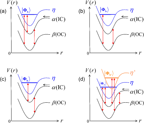
Figure 1: (color online) Multi-channel models studied in Sec. II (a–c) and Sec. IV (d). Here $r$ is the distance between the two atoms. The black curves represent the interaction potentials for the IC $\alpha$ and OC $\beta$ of the inelastic scattering processes, while the blue and orange curves represent the interaction potentials for the closed channels $\eta$ and $\eta^{\prime}$, respectively. The red arrows represent inter-channel coupling. In Sec. II, we consider cases where a bound state $|\Phi_{b}\rangle$ in the closed channel $\eta$ is coupled to both the IC $\alpha$ and OC $\beta$ (a), only coupled to the OC $\beta$ (b), or only coupled to the IC $\alpha$ (c). In Sec. IV, we consider the system where the open channels $\alpha$ and $\beta$ are coupled to two isolated bound states$|\Phi_{b}\rangle$ and $|\Phi_{b^{\prime}}\rangle$ in the $\eta$ and $\eta\prime$ channels (d).

Our results imply that two-body collisional loss in an ultracold gas may be completely suppressed when there is one OC in the inelastic scattering processes. In Sec. III we further show that when this loss is suppressed by the Fano effect, it is still possible for the elastic scattering length between the two ultracold atoms to be either large or small. That is, it is possible to obtain ultracold gases of atoms in excited internal states with strong inter-atom interactions and negligible collisional loss rates. To our knowledge, this result has not been obtained in previous studies on the control of two-body collisional loss in ultracold gases. In this section we also discuss the possible experimental realizations of our approach.

In Sec. IV we investigate the independent control of elastic and inelastic collisions between ultracold atoms. We study the system where the IC and OC are coupled to two bound states (Fig. 1(d)). We show that, for this system, when the inelastic scattering amplitude is suppressed to zero by the Fano effect, the elastic scattering length in the IC can be tuned to any value by altering the energies of these two bound states.

These results are helpful for the study of ultracold gases of atoms prepared in excited internal states. Moreover, our generalization of the Fano effect for systems with strong IC–OC coupling is also useful for the study of inelastic scattering processes in other physical systems.

II Fano effect in the system with strong IC–OC coupling

We consider the three-channel scattering problem of two ultracold atoms shown in Fig. 1(a–c). The three channels $\alpha$, $\beta$, and $\eta$ correspond to two-atom internal states $|\alpha\rangle_{I}$, $|\beta\rangle_{I}$, and $|\eta\rangle_{I}$, respectively. In natural units $\hbar=m=1$, with $m$ the single-atom mass, we can express the Hamiltonian of our system as

$$H={\bf p}^{2}+\sum_{j=\alpha,\beta,\eta}E_{j}|j\rangle_{I}\langle j|+V(r),$$ (1)

where ${\bf p}$ and ${\bf r}$ are the relative momentum and relative coordinate of the two atoms, respectively, and $r=|{\bf r}|$. The energy $E_{j}$ ($j=\alpha,\beta,\eta$) is the threshold energy of channel $j$, with $E_{\eta}>E_{\alpha}>E_{\beta}$. In Eq. (1), $V(r)$ is the interaction potential of the two atoms, and is given by

$$V(r)=\sum_{l,j=\alpha,\beta,\eta}V_{lj}(r)|l\rangle_{I}\langle j|.$$ (2)

Here $V_{jj}(r)$ ($j=\alpha,\beta,\eta$) is the potential of channel $j$, while $V_{lj}(r)=V_{jl}(r)$ ($l\neq j$) is the inter-channel coupling. For the systems shown in Fig. 1(b) and Fig. 1(c), we have $V_{\alpha\eta}=0$ and $V_{\beta\eta}=0$, respectively. In this paper we consider systems where all the components of $V$ are a real function of $r$.

We consider the case where the two atoms are incident from channel $\alpha$, and the incident state is near resonant to an isolated $s$-wave bound state $|\Phi_{b}\rangle$ in channel $\eta$. In this case, channels $\alpha$ and $\beta$ are the IC and OC of the inelastic scattering process, respectively. The $s$-wave inelastic scattering amplitude $f_{\beta\alpha}$ from channel $\alpha$ to $\beta$ can be expressed as a function of the scattering energy $E_{{\rm s}}$ and the energy $\epsilon_{b}$ of $|\Phi_{b}\rangle$. In the following we will prove that $f_{\beta\alpha}$ can always be suppressed to zero by coupling between the bound state in channel $\eta$ and the channels $\alpha$ and/or $\beta$, no matter how strong the IC–OC coupling $V_{\alpha\beta}$. That is, for any given value of $E_{{\rm s}}$, there always exists a real energy $\tilde{\epsilon}_{b}$, which leads to $f_{\beta\alpha}(E_{{\rm s}},\epsilon_{b}=\tilde{\epsilon}_{b})=0$.

In the following subsections we will first derive the analytical expression of $f_{\beta\alpha}$, and then calculate the non-diagonal element of the $K$-matrix for our system. This element is proportional to $f_{\beta\alpha}$ and easier to study. We will prove our result by analyzing the character of this $K$-matrix element.

II.1 Scattering amplitude

In this subsection we calculate the $s$-wave scattering amplitude with the method in Ref. rmp . In our system the Hilbert space $\mathcal{H}$ can be expressed as $\mathcal{H}=\mathcal{H}_{R}\otimes\mathcal{H}_{I}$, with $\mathcal{H}_{R}$ being the Hilbert space for the inter-atomic relative motion in the spatial space and $\mathcal{H}_{I}$ representing the two-atom internal state. We use $|\rangle$ to denote the state in $\mathcal{H}$, $|\rangle_{R}$ for the state in $\mathcal{H}_{R}$, and $|\rangle_{I}$ for the state in ${\cal H}_{I}$. The scattering amplitude from channel $l$ to channel $j$ ($l$, $j=\alpha,\beta$) is defined as

$$f_{jl}=-2\pi^{2}\langle\Psi_{k_{j},j}^{(0)}|V|\Psi_{k_{l},l}^{(+)}\rangle,$$ (3)

where $|\Psi_{k_{l},l}^{(+)}\rangle$ is the $s$-wave component of the out-going scattering state with respect to the incident momentum ${\bf k}_{l}$ and incident channel $l$, and the state $|\Psi_{k_{j},j}^{(0)}\rangle$ is defined as $|\Psi_{k_{j},j}^{(0)}\rangle=|\psi_{k_{j},j}^{(0)}\rangle_{R}|j\rangle_{I}$, with $|\psi_{k_{j},j}^{(0)}\rangle_{R}$ the $s$-wave component of the eigen-state $|{\bf k}_{j}\rangle_{R}$ of the relative momentum operator ${\bf p}$. Here we have $k_{l(j)}=|{\bf k}_{l(j)}|$. Notice that the $s$-wave states $|\Psi_{k_{l},l}^{(+)}\rangle$ and $|\Psi_{k_{j},j}^{(0)}\rangle$ are independent of the directions of the momentum ${\bf k}_{l}$ and ${\bf k}_{j}$, respectively. Due to energy conservation, the momentum $k_{l,j}$ satisfies

$$k_{l}^{2}+E_{l}=k_{j}^{2}+E_{j}\equiv E_{{\rm s}},$$ (4)

where $E_{{\rm s}}$ is defined as the scattering energy.

We can obtain the scattering amplitude by solving the Lippman–Schwinger equation satisfied by the scattering state $|\Psi_{k_{l},l}^{(+)}\rangle$. This equation can be expressed as (Ref. rmp , Appendix A)

$$|\Psi_{k_{l},l}^{(+)}\rangle=|\Psi_{k_{l},l}^{(\alpha\beta+)}\rangle+G^{(\alpha\beta)}(E_{{\rm s}})W|\Psi_{k_{l},l}^{(+)}\rangle,$$ (5)

where the operator $W$ is defined as

$$W=V_{\eta\alpha}(r)|\eta\rangle_{I}\langle\alpha|+V_{\eta\beta}(r)|\eta\rangle_{I}\langle\beta|+h.c.,$$ (6)

and describes the coupling between channels $\alpha,\beta$, and $\eta$. Here $|\Psi_{k_{l},l}^{(\alpha\beta+)}\rangle$ is the $s$-wave component of the out-going scattering state for the case with $W=0$, with respect to the incident channel $l$ and incident momentum ${\bf k}_{l}$, and $G^{(\alpha\beta)}(E)$ is the Green’s operator for this case. It is given by

$$G^{(\alpha\beta)}(E)=\frac{1}{E+i0^{+}-(H-W)}.$$ (7)

As shown above, we consider the case where $E_{{\rm s}}$ is near resonant to an isolated $s$-wave bound state $|\Phi_{b}\rangle\equiv|\phi_{b}\rangle_{R}|\eta\rangle_{I}$ in channel $\eta$. Here $|\phi_{b}\rangle_{I}$ satisfies the eigen-equation

$$H_{\eta}|\phi_{b}\rangle_{R}\equiv\left[{\bf p}^{2}+V_{\eta\eta}(r)+E_{\eta}\right]|\phi_{b}\rangle_{R}=\epsilon_{b}|\phi_{b}\rangle_{R}$$ (8)

of the self-Hamiltonian $H_{\eta}$ of channel $\eta$, and “near resonant” means that $E_{{\rm s}}$ is close to $\epsilon_{b}$. In this case, we can neglect the contribution from other eigen-states of $H_{\eta}$. Under this single-resonance approximation, the Green’s operator $G^{(\alpha\beta)}(E)$ can be re-expressed as

$$G^{(\alpha\beta)}(E)=\frac{1}{E+i0^{+}-h}+\frac{|\Phi_{b}\rangle\langle\Phi_{b}|}{E-\epsilon_{b}},$$ (9)

where

$$h={\bf p}^{2}+\sum_{j=\alpha,\beta}E_{j}|j\rangle_{I}\langle j|+\sum_{l,j=\alpha,\beta}V_{lj}(r)|l\rangle_{I}\langle j|$$ (10)

is the “self-Hamiltonian” of channels $\alpha$ and $\beta$. With Eq. (9), we can analytically solve the Lippman–Schwinger equation (5) for the scattering state $|\Psi_{k_{l},l}^{(+)}\rangle$, and thus obtain the $s$-wave scattering amplitude $f_{jl}(E_{{\rm s}})$ defined in Eq. (3) (Ref. rmp , Appendix B):

$$f_{jl}(E_{{\rm s}},\epsilon_{b})=f_{jl}^{(\alpha\beta)}(E_{{\rm s}})-2\pi^{2}\frac{A_{j}(E_{{\rm s}})A_{l}(E_{{\rm s}})}{B(E_{{\rm s}})-\epsilon_{b}},$$ (11)

where $f_{jl}^{(\alpha\beta)}(E_{{\rm s}})$ is the scattering amplitude for the case with $W=0$, and the functions $A_{l(j)}(E_{{\rm s}})$ and $B(E_{{\rm s}})$ are defined as

$$A_{l(j)}(E_{{\rm s}}) = \langle\Phi_{b}|W|\Psi_{k_{l(j)},l(j)}^{(\alpha\beta+)}\rangle;$$ (12)

$$B(E_{{\rm s}}) = E_{{\rm s}}-\langle\Phi_{b}|WG^{(\alpha\beta)}(E_{{\rm s}})W|\Phi_{b}\rangle.$$ (13)

II.2 $S$-matrix and $K$-matrix

In this subsection we introduce the $S$-matrix and $K$-matrix related to the $s$-wave scattering in our system. In the $s$-wave subspace the $S$-matrix is a $2\times 2$ matrix

$$S(E_{{\rm s}},\epsilon_{b})=\left[\begin{array}[]{cc}S_{\alpha\alpha}(E_{{\rm s}},\epsilon_{b}),&S_{\alpha\beta}(E_{{\rm s}},\epsilon_{b})\\ S_{\beta\alpha}(E_{{\rm s}},\epsilon_{b}),&S_{\beta\beta}(E_{{\rm s}},\epsilon_{b})\end{array}\right].$$ (14)

Here the matrix element $S_{jl}(E_{{\rm s}},\epsilon_{b})$ ($l,j=\alpha,\beta$) is related to the scattering amplitude via the relation

$$f_{jl}(E_{{\rm s}},\epsilon_{b})=\frac{S_{jl}(E_{{\rm s}},\epsilon_{b})-\delta_{jl}}{2i\sqrt{k_{l}k_{j}}}.$$ (15)

In Appendix C we show the relation between this $S$-matrix and the $S$-operator of our system st , and prove that this $S$-matrix is a unitary matrix st .

In our system the $K$-matrix is defined as kmatrix

$$K(E_{{\rm s}},\epsilon_{b}) = i\frac{1-S(E_{{\rm s}},\epsilon_{b})}{1+S(E_{{\rm s}},\epsilon_{b})}$$ (16)

$$\equiv \left[\begin{array}[]{cc}K_{\alpha\alpha}(E_{{\rm s}},\epsilon_{b}),&K_{\alpha\beta}(E_{{\rm s}},\epsilon_{b})\\ K_{\beta\alpha}(E_{{\rm s}},\epsilon_{b}),&K_{\beta\beta}(E_{{\rm s}},\epsilon_{b})\end{array}\right].$$ (19)

According to this definition, the non-diagonal elements of the $K$-matrix and $S$-matrix satisfy the relation

$$K_{\beta\alpha}=\frac{-2iS_{\beta\alpha}}{1+{\rm Det}[S]+S_{\alpha\alpha}+S_{\beta\beta}}.$$ (20)

With direct calculation based on Eqs. (11, 15) and (20), we can obtain the expression of $K_{\beta\alpha}(E_{{\rm s}},\epsilon_{b})$. Since the terms $S_{jl}$ ($j,l=\alpha,\beta$) and ${\rm Det}[S]$ in Eq. (20) are linear and quadratic functions of the scattering amplitude $f_{ij}$ given by Eq. (11), respectively, $K_{\beta\alpha}(E_{{\rm s}},\epsilon_{b})$ can be expressed as

$$K_{\beta\alpha}(E_{{\rm s}},\epsilon_{b})=\frac{F_{1}(E_{{\rm s}})\epsilon_{b}^{2}+C_{1}(E_{{\rm s}})\epsilon_{b}+D{}_{1}(E_{{\rm s}})}{F_{2}(E_{{\rm s}})\epsilon_{b}^{2}+C_{2}(E_{{\rm s}})\epsilon_{b}+D_{2}(E_{{\rm s}})},$$ (21)

and we can obtain the coefficients $C_{1,2}$, $D_{1,2}$ and $F_{1,2}$ via substituting Eqs. (11, 15) into Eq. (20). With direct calculation, we are surprised to find that the coefficients $F_{1}(E_{\rm s})$ and $F_{2}(E_{\rm s})$ of the $\epsilon_{b}^{2}$-terms in Eq. (21) are exactly zero, i.e., $F_{1}(E_{\rm s})=F_{2}(E_{\rm s})=0$. As a result, $K_{\beta\alpha}(E_{{\rm s}},\epsilon_{b})$ has a simple expression

$$K_{\beta\alpha}(E_{{\rm s}},\epsilon_{b})=\frac{C_{1}(E_{{\rm s}})\epsilon_{b}+D{}_{1}(E_{{\rm s}})}{C_{2}(E_{{\rm s}})\epsilon_{b}+D_{2}(E_{{\rm s}})},$$ (22)

where the coefficients $C{}_{1,2}(E_{{\rm s}})$ and $D_{1,2}(E_{{\rm s}})$ are given by

$$C_{1}(E_{{\rm s}}) = 2is_{\beta\alpha}(E_{{\rm s}});$$ (23)

$$C_{2}(E_{{\rm s}}) = -1-s_{\alpha\alpha}(E_{{\rm s}})s_{\beta\beta}(E_{{\rm s}})+s_{\alpha\beta}(E_{{\rm s}})s_{\beta\alpha}(E_{{\rm s}})-s_{\alpha\alpha}(E_{{\rm s}})-s_{\beta\beta}(E_{{\rm s}});$$ (24)

$$D{}_{1}(E_{{\rm s}}) = -2i\left[s_{\alpha\beta}(E_{{\rm s}})B(E_{{\rm s}})+{\cal A}_{\alpha\beta}(E_{{\rm s}})\right];$$ (25)

$$D{}_{2}(E_{{\rm s}}) = -C_{2}(E_{{\rm s}})B(E_{{\rm s}})+s_{\alpha\alpha}(E_{{\rm s}}){\cal A}_{\beta\beta}(E_{{\rm s}})+s_{\beta\beta}(E_{{\rm s}}){\cal A}_{\alpha\alpha}(E_{{\rm s}})-{\cal A}(E_{{\rm s}})\left[s_{\beta\alpha}(E_{{\rm s}})+s_{\alpha\beta}(E_{{\rm s}})\right]$$ (26)

$$+{\cal A}_{\alpha\alpha}(E_{{\rm s}})+{\cal A}_{\beta\beta}(E_{{\rm s}}),$$

with ${\cal A}_{lj}(E_{{\rm s}})=-4\pi^{2}i\sqrt{k_{j}k_{l}}A_{l}(E_{{\rm s}})A_{j}(E_{{\rm s}})$ ($l,j=\alpha,\beta$). Here, the functions $A_{l(j)}(E_{{\rm s}})$ and $B(E_{{\rm s}})$ are defined in Eqs. (12) and (13), and $s_{lj}(E_{{\rm s}})$ is the element of the $S$-matrix for the case with $W=0$.

II.3 Suppression of inelastic scattering

Based on our above results, now we prove the central result of this section.

Because the interaction potential in our system is real, the $S$-matrix $S(E_{{\rm s}},\epsilon_{b})$ is a symmetric unitary matrix (Ref. rmp , appendix C), and thus can be formally expressed as

$$S(E_{{\rm s}},\epsilon_{b})=\left(\begin{array}[]{cc}\zeta e^{i\xi}&\sqrt{1-\zeta^{2}}e^{i\xi^{\prime}}\\ \sqrt{1-\zeta^{2}}e^{i\xi^{\prime}}&-\zeta e^{-i\xi}e^{2i\xi^{\prime}}\end{array}\right),$$ (27)

where $\zeta,$ $\xi$, and $\xi^{\prime}$ are real numbers and $0<\zeta\leq 1$. Substituting Eq. (27) into Eq. (20), we find that the non-diagonal $K$-matrix element $K_{\beta\alpha}(E_{{\rm s}},\epsilon_{b})$ can be re-expressed as

$$K_{\beta\alpha}(E_{{\rm s}},\epsilon_{b})=\frac{\sqrt{1-\zeta^{2}}}{-\sin\xi^{\prime}+\zeta\sin(\xi-\xi^{\prime})},$$ (28)

and thus must be real for all values of $E_{{\rm s}}$ and $\epsilon_{b}$. Using this result and the expression (22) for $K_{\beta\alpha}(E_{{\rm s}},\epsilon_{b})$, it can be proved that (Appendix D) the ratio $D_{1}(E_{{\rm s}})/C_{1}(E_{{\rm s}})$ is always real. Thus, according to Eq. (22), non-diagonal element $K_{\beta\alpha}(E_{{\rm s}},\epsilon_{b})$ of the $K$-matrix becomes zero when the energy $\epsilon_{b}$ of the bound state in channel $\eta$ takes the value

$$\epsilon_{b}=-\frac{D_{1}(E_{{\rm s}})}{C_{1}(E_{{\rm s}})}.$$ (29)

Furthermore, according to Eqs. (20) and (15), we have

$$K_{\beta\alpha}(E_{{\rm s}},\epsilon_{b})\propto S_{\beta\alpha}(E_{{\rm s}},\epsilon_{b})\propto f_{\beta\alpha}(E_{{\rm s}},\epsilon_{b}).$$ (30)

Therefore, under the condition in Eq. (29), we have

$$f_{\beta\alpha} = 0,$$ (31)

i.e., the inelastic scattering from the IC $\alpha$ to the OC $\beta$ is completely suppressed by coupling $W$ between these two channels and the bound state $|\Phi_{b}\rangle$ in the closed channel $\eta.$ Because we do not treat the IC–OC coupling $V_{\alpha\beta}$ as a perturbation in our proof, our result is applicable to systems with arbitrarily strong IC–OC coupling.

Our proof shows that the inelastic scattering amplitude can be suppressed as long as the inter-channel coupling $W$ defined in Eq. (6) is nonzero. This is regardless of whether the coupling $V_{\beta\eta}$ between the bound state $|\Phi_{b}\rangle$ and the OC $\beta$ is zero or nonzero. When $V_{\beta\eta}\neq 0$, the suppression effect can be understood as a result of interference between the quantum transition from channel $\alpha$ to channel $\beta$ and the one from $|\Phi_{b}\rangle$ to channel $\beta$. Nevertheless, in systems with $V_{\beta\eta}=0$ and $V_{\alpha\eta}\neq 0$, i.e., the system shown in Fig. 1(c), this effect is not attributable to direct interference of these quantum transitions.

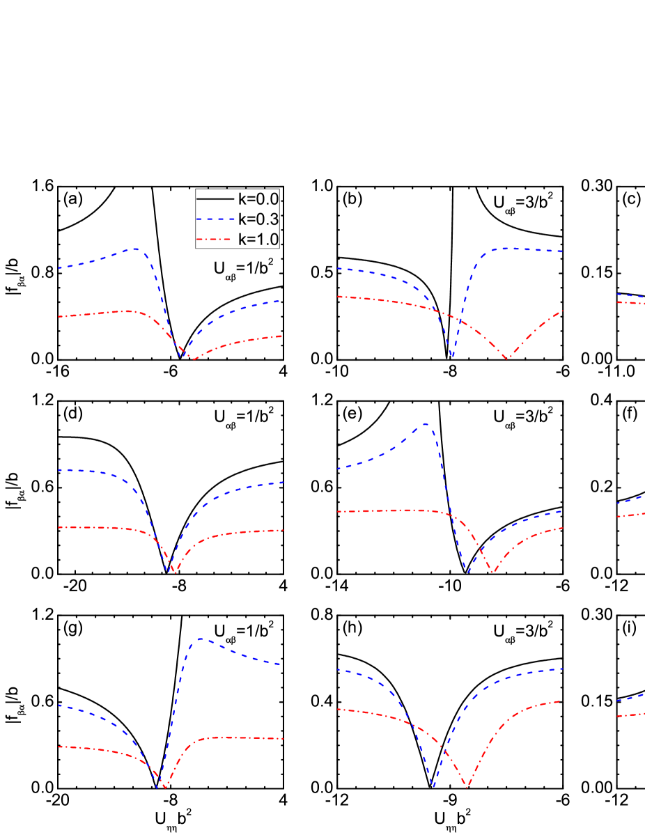
Figure 2: (color online) The absolute value $|f_{\beta\alpha}|$ of the inelastic scattering amplitude in the square-well model, as a function of the potential energy $U_{\eta\eta}$ of channel $\eta$. In (a–c), we show results for cases where $U_{\alpha\eta}=2/b^{2}$, $U_{\beta\eta}=3/b^{2}$, i.e., the cases where the closed channel $\eta$ is coupled to both IC $\alpha$ and OC $\beta$ (the cases in Fig. 1(a)). In (d–f), we show results for cases where $U_{\alpha\eta}=0$, $U_{\beta\eta}=3/b^{2}$, i.e., the cases where the closed channel $\eta$ is only coupled to OC $\beta$ (the cases in Fig. 1(b)). In (g–i), we show results for cases where $U_{\alpha\eta}=3/b^{2}$, $U_{\beta\eta}=0$, i.e., the cases where the closed channel $\eta$ is only coupled to the IC $\alpha$ (the cases in Fig. 1(c)). Here we consider systems with potential energies $U_{\alpha\alpha}=-1/b^{2}$, $U_{\beta\beta}=-2.5/b^{2}$; threshold energies $E_{\alpha}=0$, $E_{\beta}=-0.5/b^{2}$; inter-channel coupling $U_{\alpha\beta}=1/b^{2}$ (a,d,g), $3/b^{2}$ (b,e,h) and $10/b^{2}$ (c,f,i); and incident momentum $k_{\alpha}=0$ (solid black line), $0.3/b$ (dashed blue line), and $1/b$ (dash-dotted red line).

To understand the suppression effect in this special case, we consider a system where the IC–OC coupling $V_{\alpha\beta}$ is very weak and can be treated as a first-order perturbation. For this system the inelastic scattering amplitude $f_{\beta\alpha}$ can be approximated as $f_{\beta\alpha}\approx-2\pi^{2}\int drr^{2}\psi_{\beta}^{\ast}(r)V_{\alpha\beta}(r)\psi_{\alpha}(r)$, where $\psi_{\alpha(\beta)}(r)$ is the component of the $s$-wave scattering wave function in channel $\alpha$ ($\beta$) for the case with $V_{\alpha\beta}=0$. In the presence of the coupling between the IC $\alpha$ and the bound state $|\Phi_{b}\rangle$ in channel $\eta$, the wave function $\psi_{\alpha}(r)$ can be formally expressed as $\psi_{\alpha}(r)=\psi_{\alpha}^{({\rm bg})}(r)+\delta\psi_{\alpha}(\epsilon_{b},r)$. Here $\psi_{\alpha}^{({\rm bg})}(r)$ is the $s$-wave scattering wave function in channel $\alpha$ for the case with $V_{\alpha\eta}=V_{\alpha\beta}=0$, and the $\epsilon_{b}$-dependent wave function $\delta\psi_{\alpha}(\epsilon_{b},r)$ is the modification induced by $V_{\alpha\eta}$. This term describes the change of the atomic wave function in channel $\alpha$, which is induced by the second-order process where the atoms transit from channel $\alpha$ to $|\Phi_{b}\rangle$ and then return to $\alpha$. Accordingly, the inelastic scattering amplitude $f_{\beta\alpha}$ can be expressed as

$$f_{\beta\alpha}(E_{{\rm s}},\epsilon_{b}) \approx -2\pi^{2}\int drr^{2}\psi_{\beta}^{\ast}(r)V_{\alpha\beta}(r)\psi_{\alpha}^{({\rm bg})}(r)$$

$$-2\pi^{2}\int drr^{2}\psi_{\beta}^{\ast}(r)V_{\alpha\beta}(r)\delta\psi_{\alpha}(\epsilon_{b},r).$$

Eq. (LABEL:f1p) clearly shows that the inelastic scattering amplitude includes contributions from the transition processes from the states $\psi_{\alpha}^{({\rm bg})}(r)$ and $\delta\psi_{\alpha}(\epsilon_{b},r)$ to the state $\psi_{\beta}(r)$. When the interference of these two transition processes is destructive, the inelastic scattering can be suppressed. This analysis shows that, in a system where the bound state $|\Phi_{b}\rangle$ is only coupled to IC $\alpha$ and not coupled to OC $\beta$, the suppression of the inelastic scattering can be understood as a result of destructive interference between the direct transition from channel $\alpha$ to $\beta$ and the indirect transition process along the path $\alpha\rightarrow|\Phi_{b}\rangle\rightarrow\alpha\rightarrow\beta$.

II.4 Illustration

Now we illustrate our results with a simple multi-channel square-well model. In this model the potential $V_{lj}(r)$ ($l,j=\alpha,\beta,\eta$) defined in Eq. (2) is given by

$$V_{lj}(r)=\left\{\begin{array}[]{c}U_{lj},\ {\rm for}\ r<b\\ 0,\ {\rm for}\ r>b\end{array},\right.$$ (33)

with $b$ the range of these potentials. We further choose the threshold energies $E_{\alpha,\beta,\eta}$ to satisfy

$$E_{\eta}=\infty,\ E_{\alpha}=0,\ E_{\beta}<0.$$ (34)

We calculate the inelastic scattering amplitude $f_{\beta\alpha}$ from the higher channel $\alpha$ to the lower channel $\beta$, for cases where the incident state is near resonant to the lowest bound state in channel $\eta$. Figure 2 shows $|f_{\beta\alpha}|$ as a function of the potential energy $U_{\eta\eta}$ of channel $\eta$. Here, we consider cases where the closed channel $\eta$ is coupled to both the IC $\alpha$ and OC $\beta$ (Fig. 2(a-c)), and cases where channel $\eta$ is only coupled to the IC $\alpha$ (Fig. 2(d-f)) or OC $\beta$ (Fig. 2(g-i)). It is clearly shown that in all of these cases, for the system with any incident momentum $k_{\alpha}$ and IC–OC coupling $U_{\alpha\beta}$, the inelastic amplitude $f_{\beta\alpha}$ can always be suppressed to zero.

III suppression of inelastic scattering processes in ultracold gases

In this and the next section, we study the application of our results in ultracold gases. In this system, if there is only one possible two-atom inelastic scattering process (e.g., the scattering from channel $\alpha$ to channel $\beta$) then the two-body collisional loss rate is determined by the inelastic scattering amplitude $f_{\beta\alpha}$ for $E_{{\rm s}}=E_{\alpha}$, i.e., the amplitude of the threshold inelastic scattering. As was shown in Sec. II, when the open channels $\alpha$ and $\beta$ are coupled to an isolated bound state $|\Phi_{b}\rangle$ with energy $\epsilon_{b}$, this scattering amplitude can be suppressed to zero, provided that the condition (29) with $E_{{\rm s}}=E_{\alpha}$ is satisfied. With straightforward calculation, we find that this condition can be re-expressed as

$$\epsilon_{b}=\epsilon_{b}^{\ast} \equiv E_{\alpha}-\langle\Phi_{b}|WG^{(\alpha\beta)}(E_{\alpha})W|\Phi_{b}\rangle$$

$$-\frac{2\pi^{2}\langle\Phi_{b}|W|\Psi_{0,\alpha}^{(\alpha\beta+)}\rangle\langle\Phi_{b}|W|\Psi_{\sqrt{E_{\alpha}-E_{\beta}},\beta}^{(\alpha\beta+)}\rangle}{f_{\beta\alpha}^{(\alpha\beta)}(E_{\alpha})}.$$

When Eq. (LABEL:d) is satisfied, the two-body collisional loss is completely suppressed.

On the other hand, the interaction between two ultracold atoms in state $|\alpha\rangle_{I}$ can be described by the real part of the scattering length $a(\epsilon_{b})$, which is defined as

$$a(\epsilon_{b})\equiv-f_{\alpha\alpha}(E_{\alpha},\epsilon_{b}).$$ (36)

Substituting Eq. (LABEL:d) into Eq. (11) and using the optical theorem, we find that under the conditions of Eq. (LABEL:d) we have

$${\rm Re}\left[a(\epsilon_{b}^{\ast})\right] = a^{({\rm bg})}+f_{\beta\alpha}^{(\alpha\beta)}(E_{\alpha})\frac{\langle\Phi_{b}|W|\Psi_{0,\alpha}^{(\alpha\beta+)}\rangle}{\langle\Phi_{b}|W|\Psi_{\sqrt{E_{\alpha}-E_{\beta}},\beta}^{(\alpha\beta+)}\rangle};$$

$${\rm Im}\left[a(\epsilon_{b}^{\ast})\right] = 0,$$ (38)

where $a^{({\rm bg})}=-f_{\alpha\alpha}^{(\alpha\beta)}(E_{\alpha})$ is the scattering length in the system with $W=0$. Eq. (LABEL:taa2) implies that when the inelastic collision is completely suppressed, the scattering length $a(\epsilon_{b}^{\ast})$ still depends on details of the two-atom interaction potential $V(r)$ via the factors $\langle\Phi_{b}|W|\Psi_{0,\alpha}^{(\alpha\beta+)}\rangle$ and $\langle\Phi_{b}|W|\Psi_{\sqrt{E_{\alpha}-E_{\beta}},\beta}^{(\alpha\beta+)}\rangle$. In principle, it is possible for the value of ${\rm Re}\left[a(\epsilon_{b}^{\ast})\right]$ to be much larger than the range $r_{\ast}$ of $V(r)$ (e.g., the van der Waals length), or comparable to $r_{\ast}$, or much smaller than $r_{\ast}$. When ${\rm Re}\left[a(\epsilon_{b}^{\ast})\right]$ is much larger than the range $r_{\ast}$, the two atoms in channel $\alpha$ have a large probability to be close to each other. Nevertheless, because of quantum interference between the $\alpha\rightarrow\beta$ and $\eta\rightarrow\beta$ transitions, the atoms do not decay to channel $\beta$. In this case, the interaction between the two atoms in channel $\alpha$ is still strong, while the collisional loss is completely suppressed.

We illustrate our result with the square-well model in Sec. II. D. Figure 3(a–c) shows the absolute value of the inelastic scattering amplitude $f_{\beta\alpha}(E_{{\rm s}}=E_{\alpha})$ and the real part of the scattering length $a(\epsilon_{b}^{\ast})$ as functions of the potential energy $U_{\eta\eta}$ of the closed channel $\eta$, for three typical cases with the potential energy $U_{\alpha\alpha}$ of channel $\alpha$ taking the values $U_{\alpha\alpha}=-22.5/b^{2}$, $-21.779/b^{2}$, and $-21.776/b^{2}$. It is shown that in these three cases, when $|f_{\beta\alpha}|$ is suppressed to zero, the scattering length could be either comparable or much larger than the range $b$ of the interaction potential. Figure 3(d) shows the scattering length $a(\epsilon_{b}^{\ast})$ as a function of $U_{\alpha\alpha}$. It is clearly shown that for systems with different interaction potentials, the value of $a$ ranges from $-\infty$ to $+\infty$.

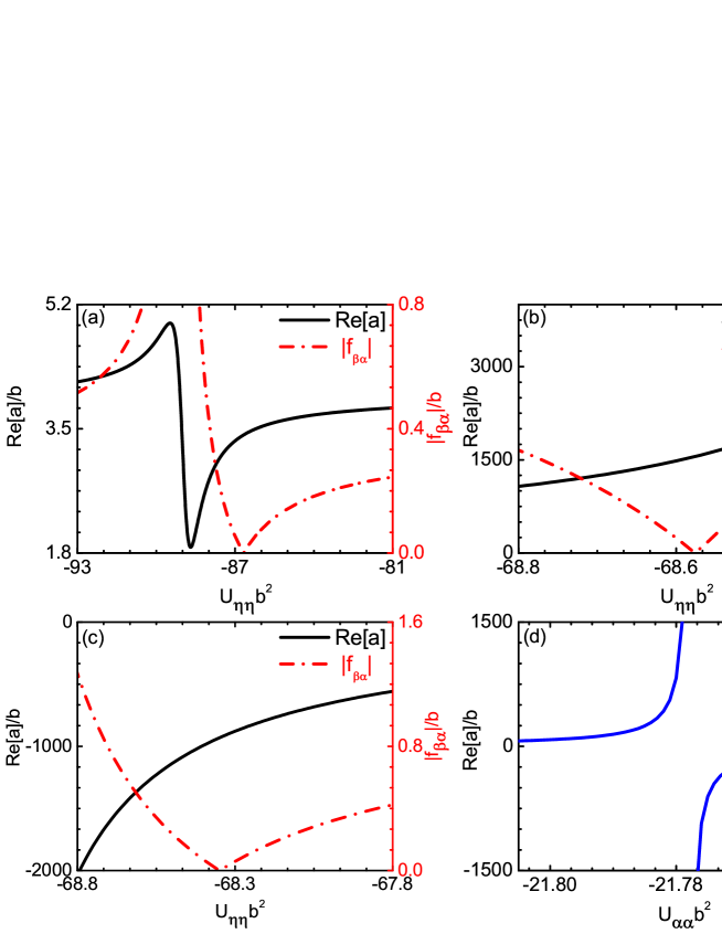
Figure 3: (color online) (a-c): The absolute value of the inelastic scattering amplitude $f_{\beta\alpha}(E_{{\rm s}}=E_{\alpha})$ and the real part of the scattering length as functions of the potential energy $U_{\eta\eta}$ of the closed channel $\eta$, for the square-well model in Sec. II. D. The potential energy $U_{\alpha\alpha}$ of channel $\alpha$ has the values $U_{\alpha\alpha}=-22.5/b^{2}$ (a), $-21.779/b^{2}$ (b), and $-21.776/b^{2}$ (c). In these three cases, when $|f_{\beta\alpha}|$ is suppressed to zero we have ${\rm Re}[a(\epsilon_{b}^{\ast})]=3.4b$ (a), $1541b$ (b), and $-931b$ (c). (d): The scattering length $a(\epsilon_{b}^{\ast})$ as a function of $U_{\alpha\alpha}$. Our calculation is done with the parameters $E_{\alpha}=0$, $E_{\beta}=-0.5/b^{2}$, $U_{\beta\beta}=U_{\alpha\beta}=U_{\beta\eta}-3/b^{2},andU_{\alpha\eta}=2/b^{2}$.

Now we investigate possible experimental realizations of our scheme. In ultracold gases of alkali atoms, the states $|\beta\rangle_{I}$, $|\alpha\rangle_{I}$, and $|\eta\rangle_{I}$ can be chosen as the lowest, second lowest, and higher two-atom hyperfine states with the same total magnetic quantum number $m_{F}^{(1)}+m_{F}^{(2)}$. Here $m_{F}^{(1(2))}$ is the magnetic quantum number of atom $1(2)$. For instance, for ultracold ⁶Li atoms, one can choose

$$|\alpha\rangle_{I}\! = \!\frac{1}{\sqrt{2}}\left[|\frac{1}{2},-\frac{1}{2}\rangle_{1}|\frac{3}{2},\frac{1}{2}\rangle_{2}-|\frac{3}{2},\frac{1}{2}\rangle_{1}|\frac{1}{2},-\frac{1}{2}\rangle_{2}\right]\!\!;$$ (39)

$$|\beta\rangle_{I}\! = \!\frac{1}{\sqrt{2}}\left[|\frac{1}{2},\frac{1}{2}\rangle_{1}|\frac{1}{2},-\frac{1}{2}\rangle_{2}-|\frac{1}{2},-\frac{1}{2}\rangle_{1}|\frac{1}{2},\frac{1}{2}\rangle_{2}\right]\!\!;$$ (40)

$$|\eta\rangle_{I}\! = \!\frac{1}{\sqrt{2}}\left[|\frac{3}{2},-\frac{1}{2}\rangle_{1}|\frac{3}{2},\frac{1}{2}\rangle_{2}-|\frac{3}{2},-\frac{1}{2}\rangle_{1}|\frac{3}{2},\frac{1}{2}\rangle_{2}\right]\!\!,$$ (41)

where $|c,d\rangle_{i}$ is the hyperfine state of the $i$-th atom with $F=c$ and $m_{F}=d$.

Since the total magnetic quantum numbers of three hyperfine channels $\alpha$, $\beta$, and $\eta$ are the same, these three channels are coupled to each other via the hyperfine spin-exchange interaction. Therefore, when we prepare the atoms in channel $|\alpha\rangle_{I}$ (e.g., prepare the ultracold ⁶Li atoms in the hyperfine states $|\frac{1}{2},-\frac{1}{2}\rangle$ and $|\frac{3}{2},\frac{1}{2}\rangle$) and the threshold energy $E_{\alpha}$ of channel $\alpha$ is near resonant to a bound state in channel $\eta$, a system shown in Fig. 1(a) can be realized.

In our system, the threshold energies $E_{\alpha,\beta}$ of channels $\alpha$, $\beta$, and the energy $\epsilon_{b}$ of the bound state in channel $\eta$ can be controlled by a static magnetic field via the Zeeman effect. Therefore, the collisional loss of atoms in channel $\alpha$ can be suppressed by tuning the magnetic field such that the condition (LABEL:d) is satisfied. When collisional loss is suppressed, the elastic scattering length between two atoms is determined by the details of the inter-atomic interactions, and can be either large or small.

One can also couple the open channel $\alpha$ or $\beta$ and the bound state $|\Phi_{b}\rangle$ in a closed hyperfine channel using a microwave field. In this way it is possible to effectively control the bound-state energy $\epsilon_{b}$ by changing the frequency of that microwave field mfr . In this case, the total magnetic quantum number of state $|\eta\rangle_{I}$ would differ from that of states $|\alpha\rangle_{I}$ and $|\beta\rangle_{I}$ mfr . In addition, in ultracold gases of alkali atoms or alkali-earth (like) atoms, a laser beam can be used to couple the open scattering channels and a bound state where one atom is in the electronic ground state and the other atom is in the electronic excited state ofr ; ofrl . However, in this system the spontaneous emission of the excited atom can also induce atomic losses. As a result, the two-body loss rate can no longer be suppressed to zero.

IV Independent control of elastic and inelastic collisions between two ultracold atoms

In the preceding sections, we studied the suppression of two-body collisional losses of ultracold atoms via the Fano effect. We show that when the collisional loss is completely suppressed, it is still possible for the two-atom scattering length, i.e., the threshold elastic scattering amplitude, to be either large or small. Nevertheless, in that system there is only one control parameter, i.e., the energy $\epsilon_{b}$ of the isolated bound state. As a result, when the collisional loss is suppressed by tuning this bound-state energy to some particular value, the scattering length of these two atoms would also be entirely fixed, and cannot be altered.

In this section, we study the independent control of elastic and inelastic collisions between two ultracold atoms. To this end, we first consider the four-channel model shown in Fig. 1(d), where the IC and OC of the inelastic scattering process are coupled to two isolated bound states, rather than a single bound state. We show that, in this “ideal” model, when the collisional loss of two atoms in the IC is suppressed by the Fano effect, the scattering length can still be tuned over a very broad region by changing the energies of the two bound states. At the end of this section we will discuss a possible experimental realization of this model.

In the model shown in Fig. 1(d), there are two bound states, $|\Phi_{b}\rangle$ and $|\Phi_{b^{\prime}}\rangle$, with energies $\epsilon_{b}$ and $\epsilon_{b^{\prime}}$, which are located in the closed channels $\eta$ and $\eta^{\prime}$, respectively. Each bound state is coupled to the IC $\alpha$ or the OC $\beta$, or both of these two open channels. It is clear that, in this system, the two-atom scattering amplitude $f_{jl}$ ($l,j=\alpha,\beta$) from channel $l$ to channel $j$ depends on both of the bound-state energies $\epsilon_{b}$ and $\epsilon_{b^{\prime}}$, i.e., we have $f_{jl}=f_{jl}[E_{{\rm s}},\epsilon_{b},\epsilon_{b^{\prime}}]$. This scattering amplitude can be calculated with the method in Sec. II. Notice that in the calculation we should replace the channel $\alpha$ in Sec. II with both the channel $\alpha$ and the bound state $|\Phi_{b^{\prime}}\rangle$ in our current system. This straightforward calculation shows that because of the Fano effect, for any given value of the energy $\epsilon_{b^{\prime}}$ of the bound state $|\Phi_{b^{\prime}}\rangle$, the threshold inelastic collision can always be completely suppressed if the energy $\epsilon_{b}$ of the bound state $|\Phi_{b}\rangle$ takes a particular $\epsilon_{b^{\prime}}$-dependent special value $\chi(\epsilon_{b^{\prime}})$, i.e., we have

$$f_{\beta\alpha}[E_{\alpha},\epsilon_{b}=\chi(\epsilon_{b^{\prime}}),\epsilon_{b^{\prime}}]=0.$$ (42)

Furthermore, when $\epsilon_{b}=\chi(\epsilon_{b^{\prime}})$, the scattering length $a$ between the two atoms becomes real, and can be expressed as a function $\bar{a}(\epsilon_{b^{\prime}})\equiv-f_{\alpha\alpha}[E_{\alpha},\epsilon_{b}=\chi(\epsilon_{b^{\prime}}),\epsilon_{b^{\prime}}]$ of the energy $\epsilon_{b^{\prime}}$. According to the direct calculation shown in Appendix E, we have

$$\bar{a}(\epsilon_{b^{\prime}})=a^{(\alpha\beta\eta^{\prime})}+\frac{A^{\prime}}{E_{\alpha}-\epsilon_{b^{\prime}}-B^{\prime}},$$ (43)

where $a^{(\alpha\beta\eta^{\prime})}$ is the scattering length in the system with $V_{\beta\eta}=V_{\alpha\eta}=0$. The expressions of the parameters $A^{\prime}$ and $B^{\prime}$ are given in Appendix E. In this appendix we also prove that $B^{\prime}$ is a $\epsilon_{b^{\prime}}$-independent real parameter. Because of this and considering Eq. (43), $\bar{a}(\epsilon_{b^{\prime}})$ can be controlled in a very broad region by tuning the bound-state energy $\epsilon_{b^{\prime}}$ in the region around $E_{\alpha}-B^{\prime}$.

Here we illustrate this control effect using calculations with a square-well potential. In our model, the total Hamiltonian is ${\bf p}^{2}+\sum_{j=\alpha,\beta,\eta,\eta^{\prime}}E_{j}|j\rangle_{I}\langle j|+\sum_{l,j=\alpha,\beta,\eta,\eta^{\prime}}V_{lj}(r)|l\rangle_{I}\langle j|$, where $V_{lj}(r)=U_{lj}$ for $r<b$, $V_{lj}(r)=0$ for $r>b$, $E_{\eta}=E_{\eta^{\prime}}=\infty$, $E_{\alpha}=0$, and $E_{\beta}<0$. In Fig. 4 we illustrate the scattering length $\bar{a}(\epsilon_{b^{\prime}})$ as a function of the energy $\epsilon_{b^{\prime}}$ of the lowest bound state in channel $\eta^{\prime}$. It is clearly shown that this scattering length can be resonantly controlled by $\epsilon_{b^{\prime}}$ or the potential energy $U_{\eta\prime\eta\prime}$ of channel $\eta\prime$.

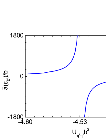
Figure 4: The elastic scattering length ${\bar{a}}(\epsilon_{b^{\prime}})\equiv-f_{\alpha\alpha}[E_{\alpha},\epsilon_{b}=\chi(\epsilon_{b^{\prime}}),\epsilon_{b^{\prime}}]$ for the square-well model in Sec. IV. Here $\epsilon_{b^{\prime}}$ is the lowest bound state in channel $\eta\prime$. The calculation is executed with the parameters $E_{\alpha}=0$, $E_{\beta}=-0.5/b^{2}$, $U_{\alpha\alpha}=-1.5/b^{2},U_{\beta\beta}=-3/b^{2}$, $U_{\alpha\beta}=U_{\beta\eta}=U_{\alpha\eta^{\prime}}=3/b^{2},andU_{\alpha\eta}=U_{\eta\eta^{\prime}}=U_{\beta\eta^{\prime}}=0$.

Here, we propose one possible experimental realization of the model discussed in this section. In an ultracold gas of alkali atoms, the states $|l\rangle_{I}$ ($l=\alpha,\beta,\eta,\eta^{\prime}$) can be chosen as a two-atom hyperfine state $|l\rangle_{I}$, which satisfies $(F_{z}^{(1)}+F_{z}^{(2)})|l\rangle_{I}=M_{l}|l\rangle_{I}$. Under the condition, $M_{\alpha}=M_{\beta}=M_{\eta}$, the channels $\alpha$, $\beta$, and $\eta$ are coupled via hyperfine interactions. Aided by the Zeeman effect, the energy $\epsilon_{b}$ of the bound state $|\Phi_{b}\rangle$ in channel $\eta$ can be controlled by a static magnetic field. In addition, with a microwave field one can further couple the open channels $\alpha$ and $\beta$ with the bound state $|\Phi_{b^{\prime}}\rangle$ in channel $\eta^{\prime}$, and effectively control the energy $\epsilon_{b^{\prime}}$ by altering the frequency of that microwave field.

V Summary

In this paper we generalize the Fano effect to systems with arbitrary IC–OC coupling strengths. We prove that in systems with one IC and one OC, when the inter-atomic interaction potential is real, the $s$-wave inelastic scattering amplitude can always be suppressed to zero by the coupling between these open channels and an isolated bound state. Using our result, we further show that when the two-body collisional loss of an ultracold gas is suppressed via the Fano effect, it is possible for the two-atom elastic scattering length to be either much larger, comparable to or smaller than the van der Waals length. We also show that when the open channels are coupled to two bound states, the elastic scattering length of the atoms in the higher open channel can be resonantly controlled, while the inelastic scattering is completely suppressed. Our results show that the Fano effect may be a very powerful technique for the suppression of collisional losses in ultracold gases. Furthermore, the generalized Fano effect we derived in Sec. II may also be useful for the study of the inelastic scattering processes in other systems.

It is pointed out that in this paper we consider systems with spherically symmetrical interaction potentials. Nevertheless, the Fano effect can also be used to suppress the collisional losses induced by anisotropic interactions, e.g., dipolar losses caused by dipole-dipole interactions Rb85loss2 ; Rb85loss3 . In these cases, although the collisional losses cannot be suppressed to zero, they can also be significantly decreased (e.g., decreased by more than one order of magnitude Rb85loss2 ; Rb85loss3 ) when one or several open channels are coupled to an isolated bound state.

Appendix A Proof of Eq. (5)

In this appendix we prove Eq. (5). According to the formal scattering theory, the scattering state $|\Psi_{k_{l},l}^{(+)}\rangle$ satisfies the equation fb

$$|\Psi_{k_{l},l}^{(+)}\rangle=\lim_{\lambda\rightarrow 0^{+}}\frac{i\lambda}{E_{{\rm s}}+i\lambda-H}|\Psi_{k_{l},l}^{(0)}\rangle,$$ (44)

where $E_{{\rm s}}$ and $H$ are defined in Eq. (65) and Eq. (1), respectively, and the state $|\Psi_{k_{l},l}^{(0)}\rangle$ is defined in Sec. II. A. Similarly, the state $|\Psi_{k_{l},l}^{(\alpha\beta+)}\rangle$, which is the $s$-wave component of the out-going scattering state for the case with $W=0$, satisfies the equation

$$|\Psi_{k_{l},l}^{(\alpha\beta+)}\rangle=\lim_{\lambda\rightarrow 0^{+}}\frac{i\lambda}{E_{{\rm s}}+i\lambda-(H-W)}|\Psi_{k_{l},l}^{(0)}\rangle.$$ (45)

Substituting the relation

$$\frac{1}{E_{{\rm s}}+i\lambda-H}=\frac{1}{E_{{\rm s}}+i\lambda-(H-W)}$$

$$+\frac{1}{E_{{\rm s}}+i\lambda-(H-W)}W\frac{1}{E_{{\rm s}}+i\lambda-H}$$ (46)

into Eq. (44), and using Eq. (45) and Eq. (7), we can obtain Eq. (5).

Appendix B Proof of Eq. (11)

In this appendix we prove Eq. (11). To this end, we substitute Eq. (9) into Eq. (5). Then we find that the solution of Eq. (5) can be expressed

$$|\Psi_{k_{l},l}^{(+)}\rangle=|\Gamma_{k_{l},l}\rangle+\kappa|\Phi_{b}\rangle,$$ (47)

where the state $|\Gamma_{k_{l},l}\rangle$ is in the subspace spanned by $|\alpha\rangle_{I}$ and $|\beta\rangle_{I}$, and $\kappa$ is a c-number. Furthermore, using Eq. (9) we can rewrite Eq. (5) as the equations of $|\Gamma_{k_{l},l}\rangle$ and $\kappa$:

$$|\Gamma_{k_{l},l}\rangle = |\Psi_{k_{l},l}^{(\alpha\beta+)}\rangle+\kappa G^{(\alpha\beta)}(E_{{\rm s}})W|\Phi_{b}\rangle,$$ (48)

$$\kappa = \frac{\langle\Phi_{b}|W|\Gamma_{k_{l},l}\rangle}{E_{{\rm s}}-\epsilon_{b}}.$$ (49)

Substituting Eq. (48) into Eq. (49), we obtain the equation

$$\kappa=\frac{\langle\Phi_{b}|W|\Psi_{k_{l},l}^{(\alpha\beta+)}\rangle}{E_{{\rm s}}-\epsilon_{b}}+\kappa\frac{\langle\Phi_{b}|WG^{(\alpha\beta)}(E_{{\rm s}})W|\Phi_{b}\rangle}{E_{{\rm s}}-\epsilon_{b}},$$ (50)

which gives

$$\kappa=\frac{\langle\Phi_{b}|W|\Psi_{k_{l},l}^{(\alpha\beta+)}\rangle}{E_{{\rm s}}-\epsilon_{b}-\langle\Phi_{b}|WG^{(\alpha\beta)}(E_{{\rm s}})W|\Phi_{b}\rangle}.$$ (51)

Substituting this result into Eq. (48), we can further derive the state $|\Gamma_{k_{l},l}\rangle$.

Using these results, we can calculate the scattering amplitude $f_{jl}(E_{{\rm s}},\epsilon_{b})$. Substituting Eq. (47) into Eq. (3), we obtain

$$f_{jl}(E_{{\rm s}},\epsilon_{b}) = -2\pi^{2}\langle\Psi_{k_{j},j}^{(0)}|(V-W)|\Gamma_{k_{l},l}\rangle$$ (52)

$$-2\pi^{2}\kappa\langle\Psi_{k_{j},j}^{(0)}|W|\Phi_{b}\rangle.$$

Substituting Eqs. (51, 48) into Eq. (52), and using the relation

$$f_{jl}^{(\alpha\beta)}(E_{{\rm s}})=-2\pi^{2}\langle\Psi_{k_{j},j}^{(0)}|(V-W)|\Psi_{k_{l},l}^{(\alpha\beta+)}\rangle$$ (53)

satisfied by the scattering amplitude $f_{jl}^{(\alpha\beta)}(E_{{\rm s}})$ for the case with $W=0$, we obtain

$$f_{jl}(E_{{\rm s}},\epsilon_{b}) = f_{jl}^{(\alpha\beta)}(E_{{\rm s}})$$

$$-2\pi^{2}\frac{\langle\Psi_{k_{j},j}^{(\alpha\beta-)}|W|\Phi_{b}\rangle\langle\Phi_{b}|W|\Psi_{k_{l},l}^{(\alpha\beta+)}\rangle}{E_{{\rm s}}-\epsilon_{b}-\langle\Phi_{b}|WG^{(\alpha\beta)}(E_{{\rm s}})W|\Phi_{b}\rangle}.$$

Here $|\Psi_{k_{j},j}^{(\alpha\beta-)}\rangle$ is the $s$-wave component of the incoming scattering state for the case with $W=0$, with respect to incident channel $j$ and incident momentum ${\bf k}_{j}$. It satisfies the Lippman–Schwinger equation

$$|\Psi_{k_{j},j}^{(\alpha\beta-)}\rangle=|\Psi_{k_{j},j}^{(0)}\rangle+G^{(\alpha\beta)}(E_{{\rm s}})^{\dagger}(V-W)|\Psi_{k_{j},j}^{(0)}\rangle$$ (55)

and the relation

$${}_{I}\langle\l|_{R}\langle{\bf r}|\Psi_{k_{j},j}^{(\alpha\beta-)}\rangle=\ _{I}\langle\l|_{R}\langle{\bf r}|\Psi_{k_{j},j}^{(\alpha\beta+)}\rangle^{\ast}$$ (56)

for $l=\alpha,\ \beta$. Here $|{\bf r}\rangle_{R}$ is the eigen-state of the relative position of the two atoms. Because of the relation (56), we have

$$\langle\Psi_{k_{j},j}^{(\alpha\beta-)}|W|\Phi_{b}\rangle=\langle\Phi_{b}|W|\Psi_{k_{j},j}^{(\alpha\beta+)}\rangle.$$ (57)

Substituting Eq. (57) into Eq. (LABEL:fjl3), we can obtain Eq. (11).

Appendix C $S$-matrix in the $s$-wave subspace

In this appendix we prove some properties of the $S$-matrix related to the $s$-wave scattering in our system, which is introduced in Sec. II. B.

We first study the relation between this $S$-matrix and the $S$-operator in our system. To this end, we introduce a state $|\Phi_{k,l}^{(0)}\rangle$ ($l=\alpha,\beta$), which is defined as $|\Phi_{k,l}^{(0)}\rangle=\sqrt{2\pi k}|\Psi_{k,l}^{(0)}\rangle$. Here $|\Psi_{k,l}^{(0)}\rangle$ is defined in Sec. II. A. It is easy to prove that

$${}_{R}\langle{\bf r}|\Phi_{k,l}^{(0)}\rangle=\frac{\sin(kr)}{2\pi\sqrt{k}r}|l\rangle_{I}.$$ (58)

This relation yields st

$$\langle\Phi_{k^{\prime},l^{\prime}}^{(0)}|\Phi_{k,l}^{(0)}\rangle=\delta_{l,l^{\prime}}\delta(E_{k,l}-E_{k^{\prime},l^{\prime}})$$ (59)

and

$$\sum_{l}\int dE|\Phi_{\sqrt{E-E_{l}},l}^{(0)}\rangle\langle\Phi_{\sqrt{E-E_{l}},l}^{(0)}|=1,$$ (60)

where the energy $E_{k,l}$ ($l=\alpha,\beta$) is defined as $E_{k,l}=k^{2}+E_{l}.$

Now let us consider the factor $\langle\Phi_{k^{\prime},l^{\prime}}^{(0)}|\hat{S}|\Phi_{k,l}^{(0)}\rangle$ ($l,l^{\prime}=\alpha,\beta$), where $\hat{S}$ is the $S$-operator of our system. It is defined as $\hat{S}=\Omega_{-}^{\dagger}\Omega_{+}$, where $\Omega_{\pm}$ are the M$\mathrm{\phi}$ller operators st . According to the formal scattering theory st , we have

$$\langle\Phi_{k^{\prime},l^{\prime}}^{(0)}|\hat{S}|\Phi_{k,l}^{(0)}\rangle=\langle\Phi_{k^{\prime},l^{\prime}}^{(-)}|\Phi_{k,l}^{(+)}\rangle,$$ (61)

with

$$|\Phi_{k,l}^{(\pm)}\rangle=\sqrt{2\pi k}|\Psi_{k,l}^{(\pm)}\rangle$$ (62)

($l=\alpha,\beta$). Here $|\Psi_{k,l}^{(+/-)}\rangle$ is the $s$-wave component of the incoming/out-going scattering state with scattering energy $E_{k,l}$ and incident channel $l$, as defined in Sec. II. A. They satisfy the Lippman–Schwinger equation

$$|\Psi_{k,l}^{(\pm)}\rangle=|\Psi_{k,l}^{(0)}\rangle+\lim_{\lambda\rightarrow 0^{+}}\frac{1}{E_{k,l}\pm i\lambda-H}V|\Psi_{k,l}^{(0)}\rangle,$$ (63)

the Schr$\ddot{{\rm o}}$dinger equation $H|\Psi_{k,l}^{(\pm)}\rangle=E_{k,l}|\Psi_{k,l}^{(\pm)}\rangle$, and the normalization condition $\langle\Psi_{k^{\prime},l^{\prime}}^{(+)}|\Psi_{k,l}^{(+)}\rangle=\langle\Psi_{k^{\prime},l^{\prime}}^{(-)}|\Psi_{k,l}^{(-)}\rangle=\langle\Psi_{k^{\prime},l^{\prime}}^{(0)}|\Psi_{k,l}^{(0)}\rangle.$ These facts yield

$$|\Phi_{k^{\prime},l^{\prime}}^{(-)}\rangle=|\Phi_{k^{\prime},l^{\prime}}^{(+)}\rangle+$$ (64)

$$\lim_{\lambda\rightarrow 0^{+}}\left(\frac{1}{E_{k^{\prime},l^{\prime}}-i\lambda-H}-\frac{1}{E_{k^{\prime},l^{\prime}}+i\lambda-H}\right)V|\Phi_{k^{\prime},l^{\prime}}^{(0)}\rangle,$$

$$H|\Phi_{k,l}^{(\pm)}\rangle=E_{k,l}|\Phi_{k,l}^{(\pm)}\rangle,$$ (65)

$$\langle\Phi_{k^{\prime},l^{\prime}}^{(+)}|\Phi_{k,l}^{(+)}\rangle=\langle\Phi_{k^{\prime},l^{\prime}}^{(-)}|\Phi_{k,l}^{(-)}\rangle=\delta(E_{k^{\prime},l^{\prime}}-E_{k,l})\delta_{l,l^{\prime}}.$$ (66)

Substituting Eq. (64) into Eq. (61), and using Eq. (66) and (65), we obtain

$$\langle\Phi_{k^{\prime},l^{\prime}}^{(0)}|\hat{S}|\Phi_{k,l}^{(0)}\rangle = \delta(E_{k^{\prime},l^{\prime}}-E_{k,l})\delta_{l,l^{\prime}}+$$

$$\left(\frac{1}{x+i0^{+}}-\frac{1}{x-i0^{+}}\right)\langle\Phi_{k^{\prime},l^{\prime}}^{(0)}|V|\Phi_{k,l}^{(+)}\rangle,$$

where $x=E_{k^{\prime},l^{\prime}}-E_{k,l}$. With the help of the relation

$$\frac{1}{x+i0^{+}}-\frac{1}{x+i0^{-}}=-2\pi i\delta(x),$$ (68)

and Eqs. (3) and (62), we can further rewrite Eq. (LABEL:ee) as

$$\langle\Phi_{k^{\prime},l^{\prime}}^{(0)}|\hat{S}|\Phi_{k,l}^{(0)}\rangle=\delta(E_{k^{\prime},l^{\prime}}-E_{k,l})S_{l^{\prime},l}(E_{k,l}),$$ (69)

where $S_{l^{\prime},l}(E_{k,l})$ is defined in Eq. (15). This is the relation between the $S$-matrix and the $S$-operator $\hat{S}$ in our system.

Now we prove the $S$-matrix is a unitary matrix. Since the $S$-operator $\hat{S}$ is a unitary operator st , it satisfies

$$\hat{S}^{\dagger}\hat{S}=1.$$ (70)

Using this result and Eqs. (59) and (60), we obtain

$$\sum_{l^{\prime\prime}}\int dE^{\prime\prime}\langle\Phi_{\sqrt{E^{\prime\prime}-E_{l^{\prime\prime}}},l^{\prime\prime}}^{(0)}|\hat{S}|\Phi_{k^{\prime},l^{\prime}}^{(0)}\rangle^{\ast}\langle\Phi_{\sqrt{E^{\prime\prime}-E_{l^{\prime\prime}}},l^{\prime\prime}}^{(0)}|\hat{S}|\Phi_{k,l}^{(0)}\rangle$$

$$=\delta_{l,l^{\prime}}\delta(E_{k^{\prime},l^{\prime}}-E_{k,l}).$$ (71)

Substituting Eq. (69) into Eq. (71), we find that the $2\times 2$ matrix with element $S_{l^{\prime},l}(E)$, i.e., the $S$-matrix we introduced in Eq. (14), is a unitary matrix.

Now we consider the $S$-matrix in the system with real interaction potential. In such a system, the $S$-operator $\hat{S}$ satisfies st

$$\langle\Phi^{\prime}|\hat{S}|\Phi\rangle=\langle\widetilde{\Phi}|\hat{S}|\widetilde{\Phi}^{\prime}\rangle,$$ (72)

where the state $|\widetilde{\Phi}\rangle$ is defined as $|\widetilde{\Phi}\rangle={\cal T}|\Phi\rangle$, with ${\cal T}$ the time-reversal operator for the spatial motion. The state $|\widetilde{\Phi}\rangle$ satisfies the relation st

$${}_{R}\langle{\bf r}|\widetilde{\Phi}\rangle={}_{R}\langle{\bf r}|\Phi\rangle^{\ast}.$$ (73)

From Eqs. (58) and (73), we know that $|\widetilde{\Phi}_{k,l}^{(0)}\rangle=|\Phi_{k,l}^{(0)}\rangle$ for $l=\alpha,\beta$. Therefore, we have

$$\langle\Phi_{k^{\prime},l^{\prime}}^{(0)}|\hat{S}|\Phi_{k,l}^{(0)}\rangle=\langle\Phi_{k,l}^{(0)}|\hat{S}|\Phi_{k^{\prime},l^{\prime}}^{(0)}\rangle.$$ (74)

This result and the relation (69) indicates that the $S$-matrix defined in Eq. (14) is a symmetric matrix for the system with real potentials.

Appendix D The ratio $D_{1}(E_{{\rm s}})/C_{1}(E_{{\rm s}})$

In this appendix we prove that the ratio $D_{1}(E_{{\rm s}})/C_{1}(E_{{\rm s}})$ appearing in Sec. II. C is real. To this end, we will first prove that all the ratios $C_{1}(E_{{\rm s}})/C_{2}(E_{{\rm s}})$, $D_{1}(E_{{\rm s}})/D_{2}(E_{{\rm s}})$, and $D_{2}(E_{{\rm s}})/C_{2}(E_{{\rm s}})$ are real.

According to Eqs. (23) and (24), the ratio $C_{1}(E_{{\rm s}})/C_{2}(E_{{\rm s}})$ is just the non-diagonal element of the $K$-matrix for the case with $W=0$. As shown in Sec. II. C, in our system this matrix element is real. Thus, $C_{1}(E_{{\rm s}})/C_{2}(E_{{\rm s}})$ is real.

Moreover, according to Eq. (22), we have $D_{1}(E_{{\rm s}})/D_{2}(E_{{\rm s}})=K_{\beta\alpha}(E_{{\rm s}},0)$. Since $K_{\beta\alpha}(E_{{\rm s}},\epsilon_{b})$ is real for any $\epsilon_{b}$, the ratio $D_{1}(E_{{\rm s}})/D_{2}(E_{{\rm s}})$ is also real.

Now we prove that $D_{2}(E_{{\rm s}})/C_{2}(E_{{\rm s}})$ is also real. We can prove this result by contradiction. To this end, we re-express Eq. (22) as

$$\left(\frac{C_{2}(E_{{\rm s}})}{C_{1}(E_{{\rm s}})}\right)K_{\beta\alpha}(E_{{\rm s}},\epsilon_{b}) = \frac{\epsilon_{b}+\left[\frac{D_{1}(E_{{\rm s}})}{C_{1}(E_{{\rm s}})}\right]}{\epsilon_{b}+\left[\frac{D_{2}(E_{{\rm s}})}{C_{2}(E_{{\rm s}})}\right]}.$$

Since both $K_{\beta\alpha}(E_{{\rm s}},\epsilon_{b})$ and $C_{2}(E_{{\rm s}})/C_{1}(E_{{\rm s}})$ are real, the right-hand side of Eq. (LABEL:kab2) is real for any $\epsilon_{b}$. Thus, if $D_{2}(E_{{\rm s}})/C_{2}(E_{{\rm s}})$ is not real, we must have $\frac{D_{1}(E_{{\rm s}})}{C_{1}(E_{{\rm s}})}=\frac{D_{2}(E_{{\rm s}})}{C_{2}(E_{{\rm s}})}$. Using Eq. (22), we find that this result yields that $K_{\beta\alpha}(E_{{\rm s}},\epsilon_{b})=C_{1}(E_{{\rm s}})/C_{2}(E_{{\rm s}})$, i.e., $K_{\beta\alpha}(E_{{\rm s}},\epsilon_{b})$ is independent of $\epsilon_{b}$. Furthermore, with Eqs. (20, 11, 15) we can express the diagonal elements of the $K$-matrix as

$$K_{\alpha\alpha}(E_{{\rm s}},\epsilon_{b}) = \frac{C_{1}^{\prime}(E_{{\rm s}})\epsilon_{b}+D_{1}^{\prime}(E_{{\rm s}})}{C_{2}(E_{{\rm s}})\epsilon_{b}+D_{2}(E_{{\rm s}})};$$ (76)

$$K_{\beta\beta}(E_{{\rm s}},\epsilon_{b}) = \frac{C_{1}^{\prime\prime}(E_{{\rm s}})\epsilon_{b}+D_{1}^{\prime\prime}(E_{{\rm s}})}{C_{2}(E_{{\rm s}})\epsilon_{b}+D_{2}(E_{{\rm s}})},$$ (77)

where the factors $C_{1}^{\prime}(E_{{\rm s}})$, $D_{1}^{\prime}(E_{{\rm s}})$, $C_{1}^{\prime\prime}(E_{{\rm s}})$, and $D_{1}^{\prime\prime}(E_{{\rm s}})$ are given by

$$C_{1}^{\prime}(E_{{\rm s}}) = -i\left[1-s_{\alpha\alpha}(E_{{\rm s}})s_{\beta\beta}(E_{{\rm s}})+s_{\alpha\beta}(E_{{\rm s}})s_{\beta\alpha}(E_{{\rm s}})-s_{\alpha\alpha}(E_{{\rm s}})+s_{\beta\beta}(E_{{\rm s}})\right];$$ (78)

$$D_{1}^{\prime}(E_{{\rm s}}) = -C_{1}^{\prime}(E_{{\rm s}})B(E_{{\rm s}})-i\left\{s_{\alpha\alpha}(E_{{\rm s}}){\cal A}_{\beta\beta}(E_{{\rm s}})+s_{\beta\beta}(E_{{\rm s}}){\cal A}_{\alpha\alpha}(E_{{\rm s}})-{\cal A}_{\alpha\beta}(E_{{\rm s}})\left[s_{\beta\alpha}(E_{{\rm s}})+s_{\alpha\beta}(E_{{\rm s}})\right]\right\}$$ (79)

$$-i{\cal A}_{\alpha\alpha}(E_{{\rm s}})+i{\cal A}_{\beta\beta}(E_{{\rm s}});$$

$$C_{1}^{\prime\prime}(E_{{\rm s}}) = -i\left[1-s_{\alpha\alpha}(E_{{\rm s}})s_{\beta\beta}(E_{{\rm s}})+s_{\alpha\beta}(E_{{\rm s}})s_{\beta\alpha}(E_{{\rm s}})+s_{\alpha\alpha}(E_{{\rm s}})+s_{\beta\beta}(E_{{\rm s}})\right];$$ (80)

$$D_{1}^{\prime\prime}(E_{{\rm s}}) = -C_{1}^{\prime\prime}(E_{{\rm s}})B(E_{{\rm s}})-i\left\{s_{\alpha\alpha}(E_{{\rm s}}){\cal A}_{\beta\beta}(E_{{\rm s}})+s_{\beta\beta}(E_{{\rm s}}){\cal A}_{\alpha\alpha}(E_{{\rm s}})-{\cal A}_{\alpha\beta}(E_{{\rm s}})\left[s_{\beta\alpha}(E_{{\rm s}})+s_{\alpha\beta}(E_{{\rm s}})\right]\right\}$$ (81)

$$i{\cal A}_{\alpha\alpha}(E_{{\rm s}})-i{\cal A}_{\beta\beta}(E_{{\rm s}}).$$

Since the $K$-matrix is a Hermitian matrix, $K_{\alpha\alpha}(E_{{\rm s}},\epsilon_{b})$ and $K_{\beta\beta}(E_{{\rm s}},\epsilon_{b})$ are real for any $\epsilon_{b}$. Therefore, with a similar method to that used above, we find that if $D_{2}(E_{{\rm s}})/C_{2}(E_{{\rm s}})$ is not real, both $K_{\alpha\alpha}(E_{{\rm s}},\epsilon_{b})$ and $K_{\beta\beta}(E_{{\rm s}},\epsilon_{b})$ are independent of $\epsilon_{b}$. Therefore, if $D_{2}(E_{{\rm s}})/C_{2}(E_{{\rm s}})$ is not real, all the $K$-matrix elements are independent of $\epsilon_{b}$. According to Eqs. (16) and (15), this result indicates that all scattering amplitudes $f_{jl}(E_{{\rm s}},\epsilon_{b})$ ($j,l=\alpha,\beta$) are independent of $\epsilon_{b}$. However, according to Eq. (11), $f_{jl}(E_{{\rm s}},\epsilon_{b})$ takes different values for different $\epsilon_{b}$. Therefore, in our system the ratio $D_{2}(E_{{\rm s}})/C_{2}(E_{{\rm s}})$ is real.

So far we have shown that the ratios $C_{1}(E_{{\rm s}})/C_{2}(E_{{\rm s}})$, $D_{1}(E_{{\rm s}})/D_{2}(E_{{\rm s}})$, and $D_{2}(E_{{\rm s}})/C_{2}(E_{{\rm s}})$ are all real. It follows that the ratio $D_{1}(E_{{\rm s}})/C_{1}(E_{{\rm s}})$ is also real.

Appendix E Eq. (43) and The Parameter $B^{\prime}$

In this appendix we will prove Eq. (43) in Sec. IV, and prove that the parameter $B^{\prime}$ is real in this equation.

Appendix F Proof of Eq. (43)

The Hamiltonian for the system in this section is

$$H_{T} = H+\left[E_{\eta^{\prime}}+V_{\eta^{\prime}\eta^{\prime}}(r)\right]|\eta^{\prime}\rangle_{I}\langle\eta^{\prime}|$$ (82)

$$+\sum_{l=\alpha,\beta}V_{l\eta^{\prime}}(r)|l\rangle_{I}\langle\eta^{\prime}|+h.c.$$

Here the Hamiltonian $H$ is defined in Eq. (1). It describes the relative kinetic energy and the interaction potential of two atoms in channels $\alpha,$ $\beta$, and $\eta$. In Eq. (82), $E_{\eta^{\prime}}$ and $V_{\eta^{\prime}\eta^{\prime}}(r)$ are the threshold energy and interaction potential of channel $\eta^{\prime}$, respectively, and $V_{\alpha\eta^{\prime}}(r)$ is the inter-channel coupling between channel $\alpha$ and $\eta^{\prime}$. Here we also assume $V_{\eta^{\prime}\eta^{\prime}}(r)$ and $V_{\alpha\eta^{\prime}}(r)$ are real functions of $r$ and tend to zero in the limit $r\rightarrow 0$.

As shown in our main text, for this system we can obtain the scattering amplitude $f_{jl}[E_{{\rm s}},\epsilon_{b},\epsilon_{b^{\prime}}]$ with the method in Sec. II. With this method we find that when the collisional decay from channel $\alpha$ to channel $\beta$ is completely suppressed, i.e., under the condition $\epsilon_{b}=\chi(\epsilon_{b^{\prime}})$, the scattering length between two ultracold atoms in channel $\alpha$ is given by

$${\bar{a}}(\epsilon_{b^{\prime}}) \equiv -f_{\alpha\alpha}[E_{\alpha},\epsilon_{b}=\chi(\epsilon_{b^{\prime}}),\epsilon_{b^{\prime}}]$$

$$= a^{(\alpha\beta\eta^{\prime})}+f_{\beta\alpha}^{(\alpha\beta\eta^{\prime})}(E_{\alpha})\frac{\langle\Phi_{b}|W|\Psi_{0,\alpha}^{(\alpha\beta\eta^{\prime}+)}\rangle}{\langle\Phi_{b}|W|\Psi_{\sqrt{E_{\alpha}-E_{\beta}},\beta}^{(\alpha\beta\eta^{\prime}+)}\rangle},$$

where the operator $W$ is defined in Eq. (6), and $|\Psi_{k,l}^{(\alpha\beta\eta^{\prime}+)}\rangle$ ($l=\alpha,\beta$) is the $s$-wave component of the out-going scattering state in the system with $W=0$, with incident momentum $k$ and incident channel $l$. In Eq. (LABEL:a3) $f_{jl}^{(\alpha\beta\eta^{\prime})}(E_{{\rm s}})$ ($j,l=\alpha,\beta$) is the scattering amplitude for the system with $W=0$, with incident channel $l$, out-going channel $j$, and scattering energy $E_{{\rm s}}$, and $a^{(\alpha\beta\eta^{\prime})}$ is defined as $a^{(\alpha\beta\eta^{\prime})}\equiv-f_{\alpha\alpha}^{(\alpha\beta\eta^{\prime})}(E_{\alpha})$.

Now we calculate the state $|\Psi_{\sqrt{E_{\alpha}-E_{\beta}},\beta}^{(\alpha\beta\eta^{\prime}+)}\rangle$. With the method in Appendix A, we can easily prove that the state $|\Psi_{\sqrt{E_{\alpha}-E_{\beta}},\beta}^{(\alpha\beta\eta^{\prime}+)}\rangle$ satisfies the equation

$$|\Psi_{\sqrt{E_{\alpha}-E_{\beta}},\beta}^{(\alpha\beta\eta^{\prime}+)}\rangle = |\Psi_{\sqrt{E_{\alpha}-E_{\beta}},\beta}^{(\alpha\beta+)}\rangle$$ (84)

$$+g^{(\alpha\beta)}(E_{\alpha})W^{\prime}|\Psi_{\sqrt{E_{\alpha}-E_{\beta}},\beta}^{(\alpha\beta\eta^{\prime}+)}\rangle,$$

where $W^{\prime}=\sum_{l=\alpha,\beta}V_{l\eta^{\prime}}(r)|l\rangle_{I}\langle\eta^{\prime}|+h.c.$, and the operator $g^{(\alpha\beta)}(E)$ is defined as $g^{(\alpha\beta)}(E)=1/[E+i0^{+}-(H_{T}-W-W^{\prime})]$. Here, the state $|\Psi_{k,l}^{(\alpha\beta+/-)}\rangle$ ($l=\alpha,\beta$) is the $s$-wave component of the out-going/incoming scattering state in the system with $W=W^{\prime}=0$, with incident momentum $k$ and incident channel $l$. Similar to that in Sec. II. A, when the incident state in channel $\alpha$ is near resonant to the bound states $|\Phi_{b}\rangle$ and $|\Phi_{b^{\prime}}\rangle$ in channels $\eta$ and $\eta^{\prime}$, the Green’s operator $g^{(\alpha\beta)}(E_{\alpha})$ can be approximated as

$$g^{(\alpha\beta)}(E_{\alpha}) = \frac{1}{E_{\alpha}+i0^{+}+h}+\frac{|\Phi_{b}\rangle\langle\Phi_{b}|}{E_{\alpha}-\epsilon_{b}}+\frac{|\Phi_{b^{\prime}}\rangle\langle\Phi_{b^{\prime}}|}{E_{\alpha}-\epsilon_{b^{\prime}}}.$$

Under this approximation we can solve Eq. (84) with the method in Appendix B, and derive the expression of $|\Psi_{\sqrt{E_{\alpha}-E_{\beta}},\beta}^{(\alpha\beta\eta^{\prime}+)}\rangle$:

$$|\Psi_{\sqrt{E_{\alpha}-E_{\beta}},\beta}^{(\alpha\beta\eta^{\prime}+)}\rangle=|\Psi_{\sqrt{E_{\alpha}-E_{\beta}},\beta}^{(\alpha\beta+)}\rangle$$

$$+\frac{g^{(\alpha\beta)}(E_{\alpha})W^{\prime}|\Phi_{b^{\prime}}\rangle\langle\Phi_{b^{\prime}}|W^{\prime}|\Psi_{k_{\beta},\beta}^{({\rm bg}+)}\rangle}{E_{{\rm s}}-\epsilon_{b^{\prime}}-\langle\Phi_{b^{\prime}}|W^{\prime}g^{(\alpha\beta)}(E_{\alpha})W^{\prime}|\Phi_{b^{\prime}}\rangle}.$$ (86)

Substituting Eq. (86) into Eq. (LABEL:a3), we obtain

$${\bar{a}}(\epsilon_{b^{\prime}})=a^{(\alpha\beta\eta^{\prime})}+\frac{A^{\prime}}{E_{\alpha}-\epsilon_{b^{\prime}}-B^{\prime}},$$ (87)

where the parameters $A^{\prime}$ and $B^{\prime}$ are given by

$$A^{\prime} = \frac{f_{\beta\alpha}^{(\alpha\beta\eta^{\prime})}(E_{\alpha})\langle\Phi_{b}|W|\Psi_{0,\alpha}^{(\alpha\beta\eta^{\prime}+)}\rangle\left[E_{{\rm s}}-\epsilon_{b^{\prime}}-\langle\Phi_{b^{\prime}}|W^{\prime}g^{(\alpha\beta)}(E_{\alpha})W^{\prime}|\Phi_{b^{\prime}}\rangle\right]}{\langle\Phi_{b}|W|\Psi_{\sqrt{E_{\alpha}-E_{\beta}},\beta}^{(\alpha\beta+)}\rangle},$$ (88)

$$B^{\prime} = \langle\Phi_{b^{\prime}}|W^{\prime}g^{(\alpha\beta)}(E_{\alpha})W^{\prime}|\Phi_{b^{\prime}}\rangle-\frac{\langle\Phi_{b}|Wg^{(\alpha\beta)}(E_{\alpha})W^{\prime}|\Phi_{b^{\prime}}\rangle\langle\Phi_{b^{\prime}}|W^{\prime}|\Psi_{\sqrt{E_{\alpha}-E_{\beta}},\beta}^{(\alpha\beta+)}\rangle}{\langle\Phi_{b}|W|\Psi_{\sqrt{E_{\alpha}-E_{\beta}},\beta}^{(\alpha\beta+)}\rangle}.$$ (89)

Eq. (87) is Eq. (43) in our main text.

Appendix G The parameter $B^{\prime}$

Now we prove that the parameter $B^{\prime}$ in Eq. (43) is real. To this end, we first prove two lemmas.

Lemma 1: The complex phase of the wave function ${}_{R}\langle{\bf r}|\Psi_{\sqrt{E_{\alpha}-E_{\beta}},\beta}^{(\alpha\beta+)}\rangle$ is ${\bf r}$-independent. That is, ${}_{R}\langle{\bf r}|\Psi_{\sqrt{E_{\alpha}-E_{\beta}},\beta}^{(\alpha\beta+)}\rangle$ can be expressed as ${}_{R}\langle{\bf r}|\Psi_{\sqrt{E_{\alpha}-E_{\beta}},\beta}^{(\alpha\beta+)}\rangle=|f({\bf r})\rangle_{I}e^{i\phi},$ where $|f({\bf r})\rangle_{I}$ is a real function of ${\bf r}$, and $\phi$ is an ${\bf r}$-independent constant.

Proof: We define an operator $g_{s}^{(\alpha\beta)}(E)$ as

$$g_{s}^{(\alpha\beta)}(E)=P_{s}g^{(\alpha\beta)}(E)P_{s},$$ (90)

where $P_{s}$ is the projection operator to the subspace of $s$-wave states. It is clear that $g_{s}^{(\alpha\beta)}(E)$ can be re-expressed as st

$$g_{s}^{(\alpha\beta)}(E) = \sum_{l=\alpha,\beta}\int d{\bf k}\frac{|\psi_{k,l}^{(\alpha\beta+)}\rangle\langle\psi_{k,l}^{(\alpha\beta+)}|}{E+i0^{+}-k^{2}-E_{l}}+\sum_{q}\frac{|B_{q}\rangle\langle B_{q}|}{E-B_{q}}$$

$$= \sum_{l=\alpha,\beta}\int d{\bf k}\frac{|\psi_{k,l}^{(\alpha\beta-)}\rangle\langle\psi_{k,l}^{(\alpha\beta-)}|}{E+i0^{+}-k^{2}-E_{l}}+\sum_{q}\frac{|B_{q}\rangle\langle B_{q}|}{E-B_{q}}.$$

Here $|B_{q}\rangle$ is the $q$-th bound state of the system with $W=W^{\prime}=0$, and $B_{q}$ is the energy of $|B_{q}\rangle$. Substituting $E=E_{\alpha}$ into Eqs. (LABEL:ga) and (LABEL:gb) and using

$$\frac{1}{z\pm i0^{+}}={\cal P}\left(\frac{1}{z}\right)\mp i\pi\delta(z),\ z\in{\rm Reals}$$ (93)

with ${\cal P}$ the principal value, we obtain

$$g_{s}^{(\alpha\beta)}(E_{\alpha})-g_{s}^{(\alpha\beta)\dagger}(E_{\alpha})$$

$$= -i4\pi^{2}\sqrt{E_{\alpha}-E_{\beta}}|\Psi_{\sqrt{E_{\alpha}-E_{\beta}},\beta}^{(\alpha\beta+)}\rangle\langle\Psi_{\sqrt{E_{\alpha}-E_{\beta}},\beta}^{(\alpha\beta+)}|$$

$$= -i4\pi^{2}\sqrt{E_{\alpha}-E_{\beta}}|\Psi_{\sqrt{E_{\alpha}-E_{\beta}},\beta}^{(\alpha\beta-)}\rangle\langle\Psi_{\sqrt{E_{\alpha}-E_{\beta}},\beta}^{(\alpha\beta-)}|.$$

Thus, we have

$${}_{R}\langle{\bf r}|\Psi_{\sqrt{E_{\alpha}-E_{\beta}},\beta}^{(\alpha\beta+)}\rangle\langle\Psi_{\sqrt{E_{\alpha}-E_{\beta}},\beta}^{(\alpha\beta+)}|{\bf r}^{\prime}\rangle_{R}$$

$$= {}_{R}\langle{\bf r}|\Psi_{\sqrt{E_{\alpha}-E_{\beta}},\beta}^{(\alpha\beta-)}\rangle\langle\Psi_{\sqrt{E_{\alpha}-E_{\beta}},\beta}^{(\alpha\beta-)}|{\bf r}^{\prime}\rangle_{R},\ {\rm for}\ \forall{\bf r},{\bf r^{\prime}}.$$

Since

$$\langle\Psi_{\sqrt{E_{\alpha}-E_{\beta}},\beta}^{(\alpha\beta-)}|{\bf r}\rangle_{R}=\langle\Psi_{\sqrt{E_{\alpha}-E_{\beta}},\beta}^{(\alpha\beta+)}|{\bf r}\rangle_{R}^{\ast},$$ (97)

the result (LABEL:psi2) implies that the complex phase of ${}_{R}\langle{\bf r}|\Psi_{\sqrt{E_{\alpha}-E_{\beta}},\beta}^{(\alpha\beta+)}\rangle$ is ${\bf r}$-independent. $\square$

Lemma 2: In our system the function

$$F(E,{\bf r},{\bf r}^{\prime}) = \sum_{l=\alpha,\beta}{\cal P}\int d{\bf k}\frac{{}_{R}\langle{\bf r}|\psi_{k,l}^{(\alpha\beta+)}\rangle\langle\psi_{k,l}^{(\alpha\beta+)}|{\bf r}^{\prime}\rangle_{R}}{E-k^{2}-E_{l}}$$ (98)

$$+\sum_{q}\frac{{}_{R}\langle{\bf r}|B_{q}\rangle\langle B_{q}|{\bf r}^{\prime}\rangle_{R}}{E-B_{q}},$$

with $|B_{q}\rangle$ defined below Eq. (LABEL:gb), is real for any energy $E$ and any positions ${\bf r}$ and ${\bf r}^{\prime}$.

Proof: Since all the potentials $V_{\alpha\beta}(r)$ are real functions of $r$, the bound-state wave function ${}_{R}\langle{\bf r}|\phi_{q}\rangle$ can be chosen to be real. Thus, the second term in the r.h.s of Eq. (98) is real. Furthermore, Eqs. (LABEL:ga) and (LABEL:gb) imply

$$\sum_{l=\alpha,\beta}{\cal P}\int d{\bf k}\frac{{}_{R}\langle{\bf r}|\psi_{k,l}^{(\alpha\beta+)}\rangle\langle\psi_{k,l}^{(\alpha\beta+)}|{\bf r}^{\prime}\rangle_{R}}{E-k^{2}-E_{l}}$$ (99)

$$= \sum_{l=\alpha,\beta}{\cal P}\int d{\bf k}\frac{{}_{R}\langle{\bf r}|\psi_{k,l}^{(\alpha\beta-)}\rangle\langle\psi_{k,l}^{(\alpha\beta-)}|{\bf r}^{\prime}\rangle_{R}}{E-k^{2}-E_{l}}.$$

From this result and Eq. (97), the first term in the r.h.s of Eq. (98) is also real. Therefore, $F(E,{\bf r},{\bf r}^{\prime})$ is a real function. $\square$

Based on these two lemmas, now we prove that the parameter $B^{\prime}$ is real. We first rewrite the expression (89) of $B^{\prime}$ as

$$B^{\prime}=\langle\Phi_{b^{\prime}}|W^{\prime}g_{s}^{(\alpha\beta)}(E_{\alpha})W^{\prime}|\Phi_{b^{\prime}}\rangle$$

$$-\frac{\langle\Phi_{b}|Wg_{s}^{(\alpha\beta)}(E_{\alpha})W^{\prime}|\Phi_{b^{\prime}}\rangle\langle\Phi_{b^{\prime}}|W^{\prime}|\Psi_{\sqrt{E_{\alpha}-E_{\beta}},\beta}^{(\alpha\beta+)}\rangle}{\langle\Phi_{b}|W|\Psi_{\sqrt{E_{\alpha}-E_{\beta}},\beta}^{(\alpha\beta+)}\rangle}.$$

(100)

Since in our system all the potentials are real, the wave functions ${}_{R}\langle{\bf r}|W^{\prime}|\Phi_{b^{\prime}}\rangle$ and ${}_{R}\langle{\bf r}|W|\Phi_{b}\rangle$ can be chosen as real functions. Therefore, our lemma 1 implies that factor $\langle\Phi_{b^{\prime}}|W^{\prime}|\Psi_{\sqrt{E_{\alpha}-E_{\beta}},\beta}^{(\alpha\beta+)}\rangle/\langle\Phi_{b}|W|\Psi_{\sqrt{E_{\alpha}-E_{\beta}},\beta}^{(\alpha\beta+)}\rangle$ is real. Furthermore, with Eq. (93) we can rewrite $g_{s}^{(\alpha\beta)}(E_{\alpha})$ as

$$g_{s}^{(\alpha\beta)}(E_{\alpha}) = \sum_{l=\alpha,\beta}{\cal P}\int d{\bf k}\frac{|\psi_{k,l}^{(\alpha\beta+)}\rangle\langle\psi_{k,l}^{(\alpha\beta+)}|}{E_{\alpha}-k^{2}-E_{l}}+\sum_{q}\frac{|\phi_{q}\rangle\langle\phi_{q}|}{E_{\alpha}-B_{q}}$$

$$-i2\pi^{2}\sqrt{E_{\alpha}-E_{\beta}}|\Psi_{\sqrt{E_{\alpha}-E_{\beta}},\beta}^{(\alpha\beta+)}\rangle\langle\Psi_{\sqrt{E_{\alpha}-E_{\beta}},\beta}^{(\alpha\beta+)}|.$$

Substituting Eq. (LABEL:gg) into Eq. (100) and using lemma 2, we can directly obtain ${\rm Im}[B^{\prime}]=0$.

References

- (1) C. J. Pethick and H. Smith, Bose-Einstein condensation in dilute gases, Cambridge University Press, 2nd edition, 2008.
- (2) K. M. Mertes, J. Merrill, R. Carretero-Gonzalez, D. J. Frantzeskakis, P. G. Kevrekidis, D. S. Hall, Phys. Rev. Lett. 99, 190402 (2007) .
- (3) S. Tojo , A. Tomiyama , M. Iwata , T. Kuwamoto , T. Hirano, Appl. Phys. B 93, 403 (2008).
- (4) F. Scazza, C. Hofrichter, M. Hfer, P. C. De Groot, I. Bloch and S. Flling, Nature Phys. 10, 779 (2014); F. Scazza, C. Hofrichter, M. Hfer, P. C. De Groot, I. Bloch and S. Flling, Nature Phys. 11, 514 (2015).
- (5) P. Halder, H. Winter, and A. Hemmerich, Phys. Rev. A 88, 063639 (2013).
- (6) John Weiner, Vanderlei S. Bagnato and Sergio Zilio, and Paul S. Julienne, Rev. Mod. Phys., 71, 1 (1999).
- (7) F. H. Mies, C. J. Williams, P. S. Julienne, and M. Krauss, . Res. Natl. Inst. Stand. Technol. 101, 521 (1996).
- (8) J. Sding, D. Gury-Odelin, P. Desbiolles, G. Ferrari, and J. Dalibard, Phys. Rev. Lett., 80, 1869 (1998).
- (9) P. A. Altin, N. P. Robins, R. Poldy, J. E. Debs, D. Dring, C. Figl, and J. D. Close, Phys. Rev. A 81, 012713 (2010).
- (10) K. Dieckmann, C. A. Stan, S. Gupta, Z. Hadzibabic, C. H. Schunck, and W. Ketterle, Phys. Rev. Lett. 89 203201 (2002).
- (11) X. Du, Y. Zhang, and J. E. Thomas, Phys. Rev. Lett., 102, 250402 (2009).
- (12) C. L. Blackley, C. Ruth Le Sueur, J. M. Hutson, D. J. McCarron, M. P. Kppinger, H. W. Cho, D. L. Jenkin, and S. L. Cornish, Phys. Rev. A 87, 033611 (2013).
- (13) J. L. Roberts, N. R. Claussen, S. L. Cornish, and C. E. Wieman, Phys. Rev. Lett. 85, 728 (2000).
- (14) J. M. Hutson, New. Jour. Phys., 9, 152 (2007) .
- (15) J. M. Hutson, M. Beyene, M. L. Gonzlez-Martnez, Phys. Rev. Lett., 103, 163201 (2009).
- (16) J. P. Burke, Jr., J. L. Bohn, B. D. Esry, and C. H. Greene, Phys. Rev. A 55, R2511 (1997).
- (17) V. A. Yurovsky and Y. B. Band, Phys. Rev. A 75, 012717 (2007).
- (18) D. M. Stamper-Kurn and M. Ueda, Rev. Mod. Phys., 85, 1191 (2011).
- (19) X. Zhang, M. Bishof, S. L. Bromley, C. V. Kraus, M. S. Safronova, P. Zoller, A. M. Rey and J. Ye, Science, , Science 345, 1467 (2014).
- (20) G. Cappellini, M. Mancini, G. Pagano, P. Lombardi, L. Livi, M. Siciliani de Cumis, P. Cancio, M. Pizzocaro, D. Calonico, F. Levi, C. Sias, J. Catani, M. Inguscio, and L. Fallani, Phys. Rev. Lett., 113, 120402 (2014); Phys. Rev. Lett. 114, 239903 (2015).
- (21) U. Fano, Phys. Rev. 15, 1866 (1961).
- (22) According to the 1st-order perturbation theory, the inelastic scattering amplitude is proportional to the transition matrix element , where is the coordinate of that scattering problem, is the IC-OC coupling, is the incident wave function, and is the component of the energy-conserved output wave function in the OC. In Ref. fano , and are denoted as and , respectively. In Sec. II of that reference, Ugo Fano calculated the modification of and the transition matrix element by the coupling to the isolated bound state.
- (23) T. Köhler, K. Gral and P. S. Julienne, Rev. Mod. Phys., 78, 1311 (2006).
- (24) J. R. Taylor, Scattering Theory, Wiley, New York, 1972.
- (25) B. Gao, Phys. Rev. A 54, 2022 (1996).
- (26) D. J. Papoular, G. V. Shlyapnikov, and J. Dalibar, Phys. Rev. A 81, 041603(R) (2010).
- (27) P. O. Fedichev, Y. Kagan, G. V. Shlyapnikov, and J. T. M. Walraven, Phys. Rev. Lett. 77, 2913 (1996).
- (28) K. Enomoto, K. Kasa, M. Kitagawa and Y. Takahashi, Phys. Rev. Lett. 101, 203201 (2008).
- (29) W. Glöckle, The Quantum Mechanical Few-Body Problem, Springer, 1983.