Subterranean production of neutrons, ${{}^{39}\text{Ar}}$ and ${{}^{21}\text{Ne}}$: Rates and uncertainties

Abstract

Accurate understanding of the subsurface production rate of the radionuclide ${{}^{39}\text{Ar}}$ is necessary for argon dating techniques and noble gas geochemistry of the shallow and the deep Earth, and is also of interest to the WIMP dark matter experimental particle physics community. Our new calculations of subsurface production of neutrons, ${{}^{21}\text{Ne}}$, and ${{}^{39}\text{Ar}}$ take advantage of the state-of-the-art reliable tools of nuclear physics to obtain reaction cross sections and spectra (TALYS) and to evaluate neutron propagation in rock (MCNP6). We discuss our method and results in relation to previous studies and show the relative importance of various neutron, ${{}^{21}\text{Ne}}$, and ${{}^{39}\text{Ar}}$ nucleogenic production channels. Uncertainty in nuclear reaction cross sections, which is the major contributor to overall calculation uncertainty, is estimated from variability in existing experimental and library data. Depending on selected rock composition, on the order of $10^{7}$–$10^{10}$ $\alpha$ particles are produced in one kilogram of rock per year (order of 1–$10^{3}$ kg^-1 s^-1); the number of produced neutrons is lower by $\sim 6$ orders of magnitude, ${{}^{21}\text{Ne}}$ production rate drops by an additional factor of 15–20, and another one order of magnitude or more is dropped in production of ${{}^{39}\text{Ar}}$. Our calculation yields a nucleogenic ${{}^{21}\text{Ne}}$/${{}^{4}\text{He}}$ production ratio of $(4.6\pm 0.6)\times 10^{-8}$ in Continental Crust and $(4.2\pm 0.5)\times 10^{-8}$ in Oceanic Crust and Depleted Mantle. Calculated ${{}^{39}\text{Ar}}$ production rates span a great range from $29\pm 9$ atoms kg-rock^-1 yr^-1 in the K–Th–U-enriched Upper Continental Crust to $(2.6\pm 0.8)\times 10^{-4}$ atoms kg-rock^-1 yr^-1 in Depleted Upper Mantle. Nucleogenic ${{}^{39}\text{Ar}}$ production exceeds the cosmogenic production below $\sim 700$ meters depth and thus, affects radiometric ages of groundwater. The ${{}^{39}\text{Ar}}$ chronometer, which fills in a gap between ${{}^{3}\text{H}}$ and ${{}^{14}\text{C}}$, is particularly important given the need to tap deep reservoirs of ancient drinking water.

1 Introduction

Argon-39 is a noble gas radionuclide with half-life of $269\pm 3$ years (NNDC, 2016) used in dating of hydrological and geological processes with timescales of a few tens to about 1000 years (Loosli, 1983; Ballentine and Burnard, 2002; Lu et al., 2014; Yokochi et al., 2012, 2013). Accurate estimates of production rates of noble gas isotopes, such as ${{}^{39}\text{Ar}}$, ${{}^{40}\text{Ar}}$ and ${{}^{21}\text{Ne}}$, in rocks are necessary for dating groundwaters and in proper interpretation of isotopic signatures of gases originating in Earth’s interior (e.g., Graham, 2002; Tucker and Mukhopadhyay, 2014).

Production of ${{}^{39}\text{Ar}}$ in the Earth’s atmosphere is dominated by the cosmogenic production channel, where ${{}^{39}\text{Ar}}$ is produced from the abundant stable ${{}^{40}\text{Ar}}$ ($\sim 1$ wt.% of atmosphere) by the cosmic ray-induced reaction ${{}^{40}\text{Ar}}(n,2n){{}^{39}\text{Ar}}$ (e.g., Loosli and Oeschger, 1968). The notation is the standard shorthand for a transfer reaction ${{}^{40}\text{Ar}}+n\rightarrow 2n+{{}^{39}\text{Ar}}$ and $n$ stands for a neutron. The ${{}^{39}\text{Ar}}$ cosmogenic production keeps the atmospheric ${{}^{39}\text{Ar}}$/Ar mass ratio at a present-day steady-state value of $(8.0\pm 0.6)\times 10^{-16}$ (Benetti et al., 2007).

Below the Earth’s surface ${{}^{39}\text{Ar}}$ can also be produced cosmogenically, by cosmic ray negative muon interactions, in particular by negative muon capture on ${{}^{39}\text{K}}$ (93.3 % of all potassium; $\mu^{-}+{{}^{39}\text{K}}\rightarrow\nu_{\mu}+{{}^{39}\text{Ar}}$). As the secondary cosmic ray muon flux drops off with depth, at depths greater than 2000 meters water equivalent (m.w.e.; $\sim 700$ m in the rock) the nucleogenic production by ${{}^{39}\text{K}}$$(n,p)$${{}^{39}\text{Ar}}$ dominates (Mei et al., 2010).

Argon extracted from several deep natural gas reservoirs shows ${{}^{39}\text{Ar}}$/Ar ratios below the atmospheric value (Acosta-Kane et al., 2008; Xu et al., 2012). For this reason, underground gas sources have attracted the attention of astroparticle physics projects that require a source of Ar with minimal radioactive ${{}^{39}\text{Ar}}$ for low-energy rare event detection of WIMP Dark Matter interactions and neutrinoless double beta decay using liquid argon detectors.

This paper provides an evaluation of the ${{}^{39}\text{Ar}}$ nucleogenic production rate for specified rock compositions by calculating the rate of ${{}^{39}\text{Ar}}$ atoms produced by naturally occurring fast neutrons. The calculation also yields results for other nuclides, in particular the rare stable ${{}^{21}\text{Ne}}$ (0.27 % of neon). We describe in detail the methods of calculation of neutron, ${{}^{21}\text{Ne}}$ and ${{}^{39}\text{Ar}}$ yields and production rates, including the use of nuclear physics software tools (SRIM, TALYS, MCNP6), and the input data, with the goal to present reproducible results. In section 2 we give the overview of the calculation. Section 3 deals with $\alpha$-particle production. Section 4 discusses production of neutrons, both by $(\alpha,n)$ reactions and by spontaneous fission. Neutron-induced reactions, in particular ${{}^{39}\text{K}}$$(n,p)$${{}^{39}\text{Ar}}$, are described in section 5. In section 6 we present the results, including coefficients for production rate evaluation (6.3) and an estimate of the uncertainty in the calculated results (6.4). A discussion follows in section 7 where we compare our calculations with recent results (Yatsevich and Honda, 1997; Mei et al., 2010; Yokochi et al., 2012, 2013, 2014, sec. 7.1), calculate the nucleogenic neutron flux out of a rock (7.2), and discuss the geochemical implications (7.3). Concluding remarks follow in section 8.

2 Overview

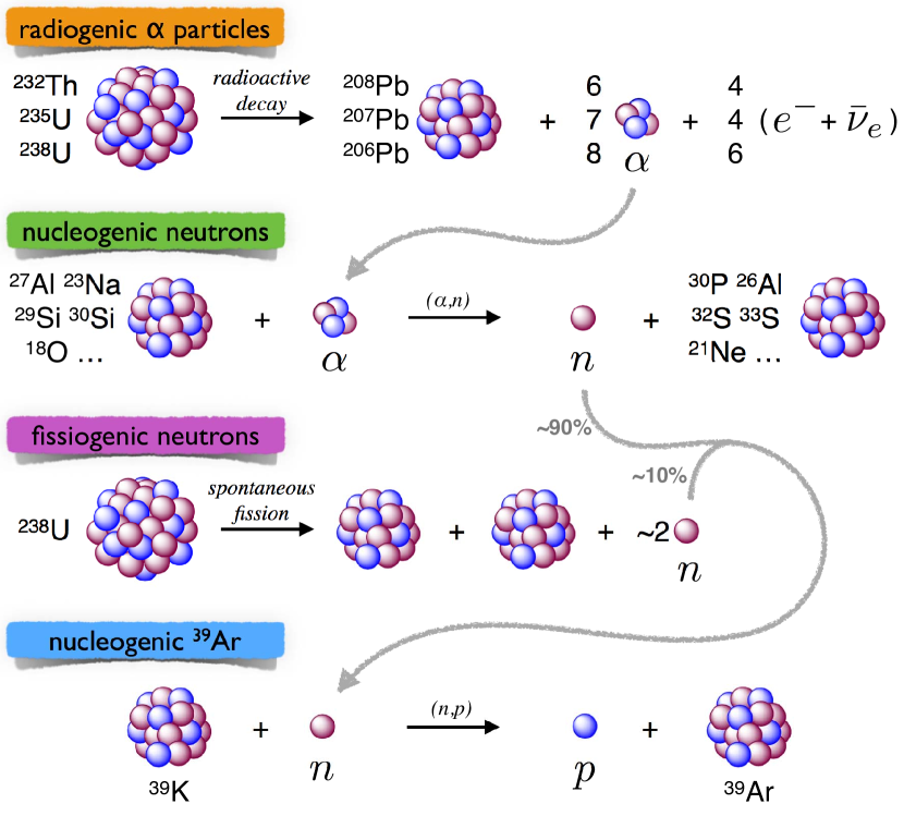
Figure 1: Overview of nucleogenic ${{}^{39}\text{Ar}}$ production.

Decays of natural radionuclides of U and Th in Earth’s interior produce $\alpha$ particles with specific known energies. The $\alpha$ particles slow down (i.e., lose kinetic energy) due to collisions with other atoms that form the silicate rock and eventually stop and form ${{}^{4}\text{He}}$ atoms by ionizing nearby matter. A small fraction ($\lesssim 10^{-6}$) of the $\alpha$ particles, before losing all their energy, participate in $(\alpha,n)$ reactions with light (atomic number $Z\lesssim 25$) target nuclides to produce fast ($\sim 1$ MeV) neutrons and product nuclides. Additional neutrons, about 10 % of the total neutrons, are produced in spontaneous fission (SF) of ${{}^{238}\text{U}}$ (mean SF neutron energy 1.7 MeV). Collectively all of these neutrons can then participate in a number of interactions, including scattering and various reactions including $(n,p)$ reactions. We are interested in the $(n,p)$ reaction on ${{}^{39}\text{K}}$ to produce ${{}^{39}\text{Ar}}$ (Figure 1).

The number of ${{}^{39}\text{Ar}}$ atoms produced per unit time per unit mass of rock is denoted $S_{39\text{Ar}}$ ($S$ for source). To calculate $S_{39\text{Ar}}$ it is necessary to know the neutron production rate as well as the neutron energy distribution. The neutron spectra are required because reaction cross sections, including that of ${{}^{39}\text{K}}$$(n,p)$${{}^{39}\text{Ar}}$, strongly depend on the energy of the incident particles. To calculate $(\alpha,n)$ neutron production and spectra, the production rate of $\alpha$ particles and their energy distribution must be known. In sections 3 to 5 we discuss the production of $\alpha$ particles, neutrons, and ${{}^{39}\text{Ar}}$. A useful byproduct of the ${{}^{39}\text{Ar}}$ calculation is the production rate of another noble gas nuclide, ${{}^{21}\text{Ne}}$, which is produced in the $(\alpha,n)$ reaction on ${{}^{18}\text{O}}$ with a limited contribution from ${{}^{24}\text{Mg}}$$(n,\alpha)$${{}^{21}\text{Ne}}$ reactions.

We evaluate the results for a number of representative rock compositions. Our selection includes the three layers of Continental Crust (CC) of Rudnick and Gao (2014), the Bulk Oceanic Crust (OC) of White and Klein (2014), and the Depleted Upper Mantle (DM) composition of Salters and Stracke (2004). Table 1 lists the elemental abundances. We also provide plug-in formulæ allowing inputs of an arbitrary elemental composition to obtain production rates.

3 Alpha-particle production

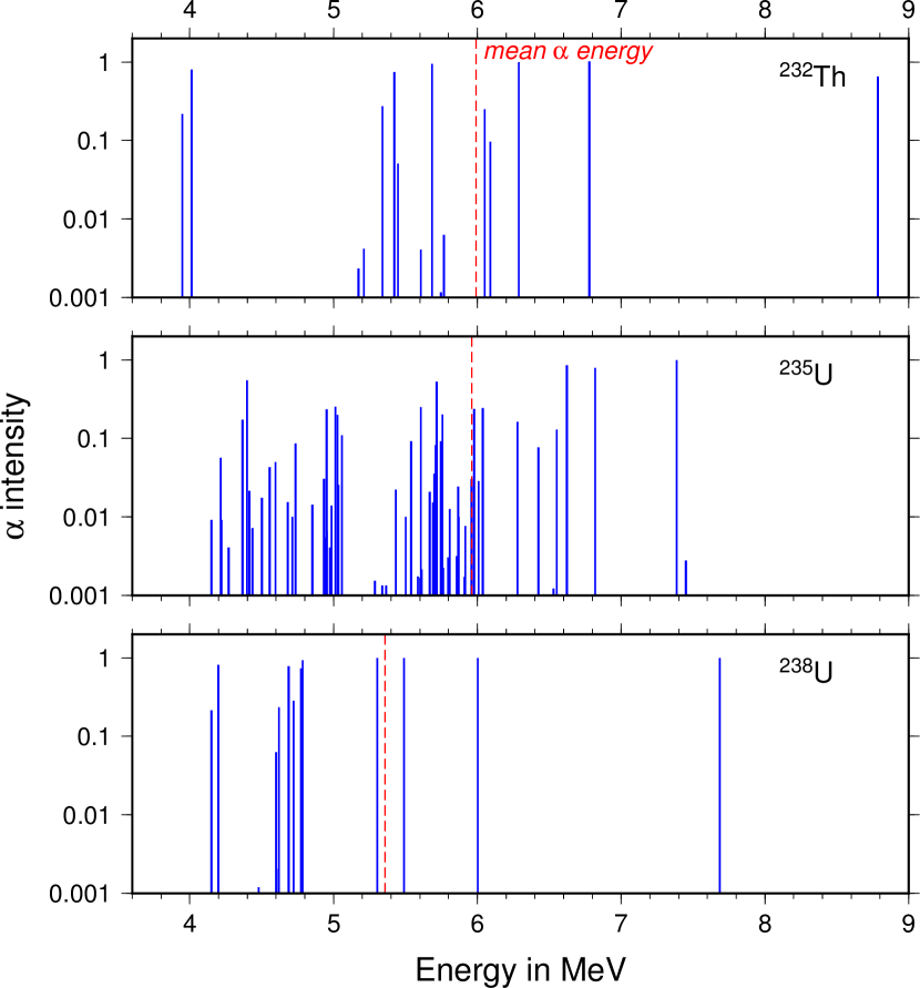
Figure 2: Natural $\alpha$ emission energy spectra. Blue spikes represent intensity of each alpha emitted. Spike intensities sum up to number of alphas emitted in particular decay chain (6, 7, 8 for ${{}^{232}\text{Th}}$, ${{}^{235}\text{U}}$, ${{}^{238}\text{U}}$, respectively). Red dashed line shows the mean energy of emitted $\alpha$ particles.

Alpha particles are produced in radioactive decays of naturally occurring ${{}^{232}\text{Th}}$, ${{}^{235}\text{U}}$, and ${{}^{238}\text{U}}$ and their daughter nuclides along the decay chains. Other natural $\alpha$ emitters are not included as their contribution is negligible (the next most potent $\alpha$ emitter, ${{}^{147}\text{Sm}}$, gives 20 times fewer $\alpha$ particles per unit mass of rock per unit time than ${{}^{235}\text{U}}$). Each individual $\alpha$-decay emits one $\alpha$ particle with specific energies, given by the decay scheme which is characterized by the energy levels and intensities. We use decay data—half-lives, branching ratios, $\alpha$ energy levels, $\alpha$ intensities—from “Chart of Nuclides” available at the National Nuclear Data Center website (NNDC, 2016). The resulting $\alpha$ energy spectra are shown in Figure 2. Tabulated $\alpha$ energies and intensities as well as charts of decay networks can be found in Supplementary Materials. The maximum $\alpha$ energy is 8.78 MeV from decay of ${{}^{212}\text{Po}}$ in the thorium decay chain. The mean $\alpha$ energy in ${{}^{232}\text{Th}}$, ${{}^{235}\text{U}}$, and ${{}^{238}\text{U}}$ chains is 6.0, 6.0, and 5.4 MeV, respectively.

Decays of ${{}^{232}\text{Th}}$, ${{}^{235}\text{U}}$, and ${{}^{238}\text{U}}$ produce $n_{\alpha}=6$, 7, and 8 $\alpha$’s per chain. The $\alpha$ production rate $S_{\alpha}$—number of $\alpha$ particles produced per unit time in unit mass of rock—of each decay chain is proportional to the elemental abundance (mass fraction) $A$ of the parent (Th or U) and is obtained by simple multiplication,

$$S_{\alpha}=n_{\alpha}A\lambda\frac{XN_{A}}{M}=n_{\alpha}A\mathcal{C},$$ (1)

where we have introduced the per-decay-to-rate conversion factor $\mathcal{C}$,

$$\mathcal{C}\equiv\lambda\frac{XN_{A}}{M},$$ (2)

in which $\lambda$ is the decay constant and the fraction $XN_{A}/M$ is the number of parent nuclide atoms per unit mass of element (e.g., number of ${{}^{238}\text{U}}$ atoms per 1 kg of natural U) where $X$ is natural isotopic composition (mole fraction), $M$ is standard atomic weight, and $N_{A}$ is Avogadro’s number (see Table 2 for values). The three equations (1), one for each decay chain, can be recast into one plug-in formula to calculate $\alpha$ production rate from uranium concentration in ppm and Th/U ratio,

$$S_{\alpha}\left[\frac{\#}{\text{kg-rock\,s}}\right]=\left(103+24.3\frac{A_{\text{Th}}}{A_{\text{U}}}\right)A_{\text{U}}\text{[ppm]}.$$ (3)

Alpha production rates $S_{\alpha}$ are evaluated in Table 3 for the representative rock compositions.

Each $\alpha$ particle is emitted with a specific initial kinetic energy $E_{\alpha_{0}}$ (Figure 2). It progressively loses its energy, mostly by inelastic scattering on atomic electrons and elastic scattering on nuclei. The range of an $\alpha$ particle, i.e., how far it travels before stopping, is obtained by integration along its path,

$$\text{Range}(E_{\alpha_{0}})=\int\limits_{E_{\alpha_{0}}}^{0}\mathrm{d}x=\int\limits_{0}^{E_{\alpha_{0}}}\frac{\mathrm{d}E_{\alpha}}{\left(-\frac{\mathrm{d}E_{\alpha}}{\mathrm{d}x}\right)},$$ (4)

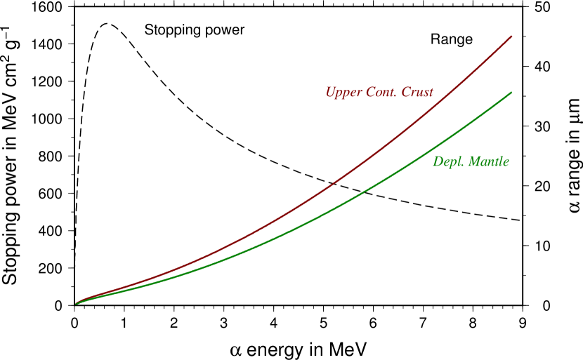
Figure 3: Mass stopping power $-\rho^{-1}\mathrm{d}E/\mathrm{d}x$ for an $\alpha$ particle in rock (dashed line, left vertical axis) and range of $\alpha$ particle (eqn. 4, solid lines, right vertical axis) as a function of $\alpha$ energy. Range plotted up to maximum energy of a natural $\alpha$ particle (8.78 MeV from decay of ${{}^{212}\text{Po}}$). The difference between range in Upper Cont. Crust (red) and Depleted Mantle (green) simply reflects the difference in rock density (Table 1). Curves for Middle and Lower CC and OC fall between the two shown.

and is a function of the initial energy of the $\alpha$ particle in a given material. The material property $-\mathrm{d}E_{\alpha}/\mathrm{d}x$ is the linear stopping power. We use the SRIM software (srim.org; Ziegler et al., 2008), version SRIM-2013.00, to obtain the mass stopping power $-\rho^{-1}\mathrm{d}E_{\alpha}/\mathrm{d}x$, where $\rho$ is rock density (listed in Table 1). Mass stopping power is essentially identical for all rock compositions we consider and its energy dependence is plotted in Figure 3. The range of an average-energy natural $\alpha$ ($\sim 6$ MeV) in the rock is about 25 $\mu$m (Figure 3). We assume that $\alpha$ particle propagation is isotropic with no channeling in the crystal lattice on the grain scale.

4 Neutron production

The overall neutron production rate $S_{n}$—number of neutrons produced per unit time in unit mass of rock—in each decay chain is calculated from

$$S_{n}=A\mathcal{C}Y,$$ (5)

where the neutron yield $Y$, i.e., the number of neutrons produced from decay or fission of one atom of parent nuclide, is the sum of contributions from $(\alpha,n)$ reactions on various target nuclides and from spontaneous fission,

$$Y=\sum\limits_{i}^{\text{\#\,targets}}Y_{\alpha,n}^{i}+Y_{\text{SF}}.$$ (6)

We now calculate the individual neutron yields. Energy spectra of the neutrons produced via various production pathways are also discussed in the following sections.

4.1 Neutrons from $(\alpha,n)$ reactions

Neutron production by $(\alpha,n)$ was comprehensively described and quantified by Feige et al. (1968). Before an $\alpha$ particle loses all its kinetic energy, it can enter another atom’s nucleus to form a compound nucleus. The $\alpha$ has to have enough energy to overcome the Coulomb barrier, i.e., the electromagnetic repulsion between the target nucleus and the $\alpha$ particle. The Coulomb barrier height $V_{C}$ is estimated from

$$V_{C}=\frac{1}{4\pi\epsilon_{0}}\frac{q_{1}q_{2}}{r}=1.4400\frac{Z_{1}Z_{2}}{R_{int}\text{[fm]}}\,\text{MeV}=\frac{1.4400\,Z_{1}Z_{2}}{1.2(\mathcal{A}_{1}^{1/3}+\mathcal{A}_{2}^{1/3})}\,\text{MeV},$$ (7)

where indices 1 and 2 refer to projectile and target, $\epsilon_{0}$ is vacuum permittivity, $q$ is electric change, $r$ is distance, $Z$ is atomic number, $R_{int}$ (in femtometers) is the interaction radius taken as the sum of the two atomic radii, which in turn are approximated by a common empirical formula assuming nuclear volume to be proportional to the mass number $\mathcal{A}$. As the Coulomb barrier height is proportional to the charge of the target nucleus, only relatively low $Z$ target nuclides allow for compound nucleus formation from natural $\alpha$ particles. Even though the compound nucleus can form with $\alpha$ energies below the Coulomb barrier due to quantum tunneling effect, the interaction cross section drops rapidly.

The compound nucleus is considered a short-lived intermediate state and from this compound nucleus there are many possible channels that form various products nuclides. At energies of natural $\alpha$ particles, the most common outcome is that the compound nucleus then sheds a neutron to form a product nucleus. This constitutes an $(\alpha,n)$ reaction. For example, $\alpha+{{}^{18}\text{O}}$ form a compound ${{}^{22}\text{Ne}}^{*}$, which then emits a neutron to produce the ${{}^{21}\text{Ne}}$ product or, in shorthand, ${{}^{18}\text{O}}$$(\alpha,n)$${{}^{21}\text{Ne}}$. The majority of the relevant $(\alpha,n)$ reactions are endothermic, i.e., their $Q$ value is negative ($Q$ value being reactant minus product rest masses), and the incoming $\alpha$ particle has to have energy above a threshold $E_{th}$ for the reaction to proceed. Specifically, the kinetic energy in the center-of-mass system before interaction has to be larger than $|Q|$ if $Q<0$. In the laboratory reference frame, this translates into a relation for the threshold energy of an endothermic reaction

$$E_{th}=-\frac{m_{1}+m_{2}}{m_{2}}Q,$$ (8)

where $m_{1}$ is the rest mass of projectile and $m_{2}$ that of target nuclide.

The Coulomb barrier and threshold energy result in a strong energy dependence of the $(\alpha,n)$ reaction cross section. Based on the magnitude of cross sections and the abundance of a particular nuclide in natural rocks, we identify 14 target nuclides that are important for $(\alpha,n)$ neutron production in natural rocks. They are listed in Table 4 together with the $(\alpha,n)$ reaction $Q$ values, threshold energies $E_{th}$ (8), and Coulomb barrier heights $V_{C}$ (7).

The chance that an $\alpha$ particle, emitted with initial energy $E_{\alpha_{0}}$, participates in an $(\alpha,n)$ reaction on a light target nuclide $i$ is quantified by the thick target—meaning that the $\alpha$ stops within the medium—neutron production function

$$P_{i}(E_{\alpha_{0}})=N_{i}\int\limits_{E_{\alpha_{0}}}^{0}\frac{\sigma_{\alpha,n}^{i}(E_{\alpha})}{\frac{\mathrm{d}E_{\alpha}}{\mathrm{d}x}}\mathrm{d}E_{\alpha},$$ (9)

where $N_{i}$ is the atomic density of nuclide $i$ (# atoms of $i$ per unit volume) and $\sigma_{\alpha,n}^{i}$ is the $(\alpha,n)$ cross section for nuclide $i$. To get from neutron production function to $(\alpha,n)$ neutron yield consists of, for each decay chain and target nuclide $i$, accounting for all $\alpha$ decays and $\alpha$ energy levels within each decay, giving

$$Y_{\alpha,n}^{i}=\sum\limits_{k=1}^{\text{decays}}b_{k}\sum\limits_{l=1}^{\text{levels}}f_{kl}P_{i}(E_{kl}),$$ (10)

where $b_{k}$ accounts for decay chain branching and $f_{kl}$ is the $\alpha$ intensity of level $l$ in decay $k$ with $\alpha$ energy $E_{kl}$.

To calculate the $(\alpha,n)$ neutron energy spectra, we evaluate the differential neutron production function $\mathrm{d}P_{i}/\mathrm{d}E_{n}$,

$$\frac{\mathrm{d}P_{i}}{\mathrm{d}E_{n}}(E_{\alpha_{0}},E_{n})=N_{i}\int\limits_{E_{\alpha_{0}}}^{0}\frac{\frac{\mathrm{d}\sigma_{\alpha,n}^{i}}{\mathrm{d}E_{n}}(E_{\alpha},E_{n})}{\frac{\mathrm{d}E_{\alpha}}{\mathrm{d}x}}\mathrm{d}E_{\alpha},$$ (11)

which is an equation analogous to (9) except that it calls for the neutron spectrum (or differential cross section) $\mathrm{d}\sigma_{\alpha,n}^{i}/\mathrm{d}E_{n}$, instead of the integrated cross section $\sigma_{\alpha,n}^{i}$ ($E_{n}$ denotes neutron energy). To obtain the yield spectrum (or differential yield) $\mathrm{d}Y_{\alpha,n}^{i}/\mathrm{d}E_{n}$, we follow the analogy through equation (10). Similar thick target methods for $\alpha$ particles have been used to study nuclear reaction rates for astrophysics (Roughton et al., 1983), and these methods have been used for thermonuclear reactions in energetic plasmas (Intrator et al., 1981).

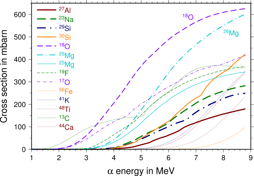
Figure 4: Energy dependent $(\alpha,n)$ cross sections $\sigma_{\alpha,n}$ for target nuclides considered in this study as calculated by TALYS version 1.6. One mbarn = $10^{-27}$ cm².

We use the nuclear physics code TALYS (www.talys.eu; Koning et al., 2008), version 1.6 released on December 23, 2013, to calculate the $(\alpha,n)$ neutron production cross sections $\sigma_{\alpha,n}^{i}$ as well as the emitted neutron energy spectra $\mathrm{d}\sigma_{\alpha,n}^{i}/\mathrm{d}E_{n}$. We use the default TALYS input parameters except for allowing the width fluctuation corrections calculated using the Moldauer model at all energies (see the TALYS documentation for details). An example of our TALYS input file is provided in Supplementary Materials. The TALYS-calculated $(\alpha,n)$ cross sections for all considered target nuclides are plotted in Figure 4.

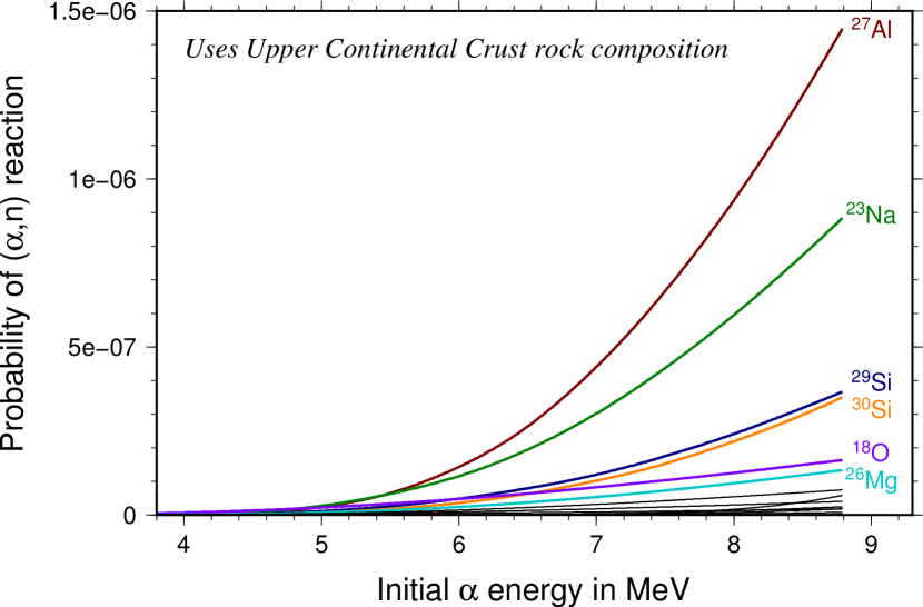
Figure 5: Thick target $(\alpha,n)$ neutron production function $P$ (i.e., neutron yield per one $\alpha$ particle; eqn. 9) plotted against the initial $\alpha$ energy for various target nuclides. Curves for the six most neutron producing targets are labeled and color-coded. Remaining targets plotted as thin black lines. The Upper CC rock composition is used. Different amplitudes for various target nuclides stem from the combined effect of elemental abundance, natural isotopic composition, and energy dependence of $(\alpha,n)$ cross section.

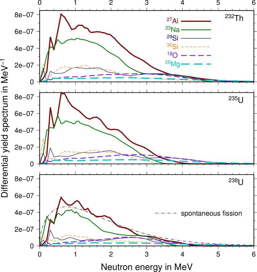
Figure 6: $(\alpha,n)$ neutron yield spectra $\mathrm{d}Y_{\alpha,n}/\mathrm{d}E_{n}$ plotted against neutron energy for each decay chain and six most neutron producing targets. The fission neutron yield spectrum $\mathrm{d}Y_{\text{SF}}/\mathrm{d}E_{n}$ is also plotted (non-negligible only in ${{}^{238}\text{U}}$ decay). The Upper CC rock composition is used. Area below each curve integrates to the neutron yield $Y_{\alpha,n}$ or $Y_{\text{SF}}$ (i.e., neutrons produced per decay of one atom of parent nuclide).

The calculated neutron production function $P_{i}$ (9) of various target nuclides is presented in Figure 5. The figure shows the relative importance of various target nuclides, which depends both on the cross section magnitude and the nuclide abundance in the rock. Figure 6 shows the neutron yield spectra $\mathrm{d}Y_{\alpha,n}^{i}/\mathrm{d}E_{n}$ for each decay chain and target nuclide from each of the three actinides. The mean energy of neutrons generated by $(\alpha,n)$ reactions is 1.8 MeV in ${{}^{232}\text{Th}}$ decay chain, 1.6 MeV in ${{}^{235}\text{U}}$ chain, and 1.7 MeV in ${{}^{238}\text{U}}$ chain.

4.2 Neutrons from spontaneous fission

Spontaneous fission of ${{}^{238}\text{U}}$ produces 2.07 neutrons per fission (Shultis and Faw, 2002) and the SF branching ratio is $5.5\times 10^{-7}$ (NNDC, 2016). The fission neutron spectrum is approximated by the Watt fission spectrum with neutron energy distribution following $\exp(-E_{n}/a)\sinh\sqrt{bE_{n}}$ with parameters $a=0.6483$ MeV and $b=6.811$ MeV (SOURCES-4C, 2002), resulting in a mean SF neutron energy of 1.7 MeV. The fission neutron yield spectrum $\mathrm{d}Y_{\text{SF}}/\mathrm{d}E_{n}$ is included in Figure 6. The number of neutrons produced in spontaneous fission of ${{}^{232}\text{Th}}$ and ${{}^{235}\text{U}}$, as well as other nuclides with non-zero SF branching fraction in the decay chains (${{}^{234}\text{U}}$, ${{}^{230}\text{Th}}$, ${{}^{231}\text{Pa}}$), is negligible compared to neutrons from $(\alpha,n)$ reactions.

5 Neutron-induced reactions: $(n,p)$ and $(n,\alpha)$

To quantify the last step in the nuclear reaction sequence of ${{}^{39}\text{Ar}}$ production, the ${{}^{39}\text{K}}$$(n,p)$${{}^{39}\text{Ar}}$ exothermic reaction (Table 4), we use MCNP6, version MCNP6_Beta3, a general-purpose Monte Carlo N-Particle transport code developed at Los Alamos National Laboratory (mcnp.lanl.gov). MCNP6 allows us to calculate the ${{}^{39}\text{Ar}}$ yield per one neutron where we specify the neutron energy spectrum for each of the $(\alpha,n)$ and SF neutron production channels. An example of our MCNP6 input file is provided in Supplementary Materials. In addition to ${{}^{39}\text{Ar}}$ yields, we also use MCNP6 to calculate the ${{}^{21}\text{Ne}}$ yield from the ${{}^{24}\text{Mg}}$$(n,\alpha)$${{}^{21}\text{Ne}}$ endothermic reaction (Table 4). From these nuclide yields and neutron production rates discussed in previous section, we can evaluate the ${{}^{39}\text{Ar}}$ and ${{}^{21}\text{Ne}}$ production rates $S_{39\text{Ar}}$ and $S_{21\text{Ne}}$.

6 Results

6.1 Neutron yields and production rates

The calculated yields $Y$ and production rates $S_{n}$ of neutrons produced by both $(\alpha,n)$ reactions and by spontaneous fission are reported in Table 5. For the Upper CC compositions we report detailed results for each $(\alpha,n)$ target nuclide and each natural decay chain to show the relative importance of various neutron production channels. For the remaining representative compositions, only the ${{}^{18}\text{O}}$$(\alpha,n)$${{}^{21}\text{Ne}}$, SF, and total neutron yields are presented. The maximum neutron yields are of the order of $3\times 10^{-6}$ neutrons per decay of 1 atom of long-lived radionuclide. With Upper CC composition, spontaneous fission is responsible for 11 % of total neutrons produced; with other compositions the SF contribution ranges from 8 to 12 %. Of $(\alpha,n)$ target nuclides in Upper CC rocks, ${{}^{27}\text{Al}}$ produces the most neutrons at 32 % of total, followed by ${{}^{23}\text{Na}}$ at 23 %, ${{}^{29}\text{Si}}$ at 9.2 %, ${{}^{30}\text{Si}}$ at 7.8 %, ${{}^{18}\text{O}}$ at 7.0 %, ${{}^{26}\text{Mg}}$ at 4.0 % and ${{}^{25}\text{Mg}}$ at 2.4 %. These proportions obviously vary with composition, however, these seven target nuclides + SF neutrons account for at least 96 % of neutrons produced for all representative compositions we use. With the magnesium-rich DM composition, Mg nuclides alone account for 69 % of neutrons. In terms of contributions of decay chains, with Upper CC composition ${{}^{232}\text{Th}}$ accounts for 57 % and ${{}^{238}\text{U}}$ for 41 % of neutrons produced. Again, exact proportions vary with composition but the trend, ${{}^{232}\text{Th}}>{{}^{238}\text{U}}\gg{{}^{235}\text{U}}$, holds.

6.2 ${{}^{39}\text{Ar}}$ and ${{}^{21}\text{Ne}}$ yields and production rates

The largest $(n,p)$ and $(n,\alpha)$ nuclide yields (per neutron per elemental weight fraction of reacting nuclide, i.e., K or Mg) are obtained with highest energy neutron spectra, coming from exothermic $(\alpha,n)$ reactions with positive $Q$ values. That is, from $(\alpha,n)$ target nuclides ${{}^{13}\text{C}}$, ${{}^{17}\text{O}}$, ${{}^{26}\text{Mg}}$, and in particular ${{}^{25}\text{Mg}}$, which provides the highest energy neutrons. The maximum nuclide yields are of the order of 0.4 per neutron per weight fraction of K for ${{}^{39}\text{Ar}}$ and 0.05 per neutron per weight fraction of Mg for ${{}^{21}\text{Ne}}$. The production rates, per year per kilogram of rock, also factor in the relative importance of neutron production channels. Therefore, the seven most neutron producing nuclides (${{}^{27}\text{Al}}$, ${{}^{23}\text{Na}}$, ${{}^{29}\text{Si}}$, ${{}^{30}\text{Si}}$, ${{}^{18}\text{O}}$, ${{}^{26}\text{Mg}}$, ${{}^{25}\text{Mg}}$) and SF are also responsible for most of ${{}^{39}\text{Ar}}$ production. Neon-21 production by $(n,\alpha)$ is dominated by $(\alpha,n)$ neutrons from ${{}^{25}\text{Mg}}$ (55–81 % of ${{}^{21}\text{Ne}}$ produced depending on chosen composition). The results for ${{}^{39}\text{Ar}}$ and ${{}^{21}\text{Ne}}$ production rates are reported in Table 5.

Table 6 summarizes the subsurface production of $\alpha$ particles, neutrons, ${{}^{21}\text{Ne}}$, and ${{}^{39}\text{Ar}}$. Depending on selected rock composition, on the order of $10^{7}$–$10^{10}$ $\alpha$ particles are produced in one kilogram of rock per year. The number of neutrons produced is lower by $\sim 6$ orders of magnitude, ${{}^{21}\text{Ne}}$ production rate drops by an additional factor of 15–20, and production rate of ${{}^{39}\text{Ar}}$ decreases by at least another order of magnitude. In Table 6 we include production rates of ${{}^{4}\text{He}}$, ${{}^{21}\text{Ne}}$, and ${{}^{39}\text{Ar}}$ in units of cm³ STP per year per gram of rock, in order to facilitate easier comparison of our results to previous work.

6.3 Coefficients for plug-in formulæ

In Table 7 we provide coefficients $\chi$ that one can use to calculate subsurface neutron production, ${{}^{21}\text{Ne}}$ production by $(\alpha,n)$ and nucleonic ${{}^{39}\text{Ar}}$ production in a rock of arbitrary composition. The word “arbitrary” should be qualified with “while close enough to a natural rock composition”. To indicate what “close enough” means, let us state that while the provided coefficients are based on a calculation with Upper CC composition, the empirical formulas yield a result within 1 % of the actual value for all rock compositions we use here (Upper, Middle, and Lower CC, Bulk OC, Depleted Upper Mantle). The one exception is ${{}^{39}\text{Ar}}$ production evaluation for DM composition, where the Upper CC coefficients overestimate ${{}^{39}\text{Ar}}$ by 8 %.

As an example, we use these coefficients to evaluate the neutron and ${{}^{39}\text{Ar}}$ production rate in the ${{}^{18}\text{O}}$ $(\alpha,n)$ target nuclide channel with $\alpha$ particles from ${{}^{238}\text{U}}$ decay chain in a rock with Upper CC composition. The appropriate neutron production coefficient $\chi_{n}({{}^{18}\text{O}},{{}^{238}\text{U}})$ in Table 7 is $2.27\times 10^{8}$ and the neutron production rate is evaluated, using elemental abundances from Table 1, as

$$\begin{split}S_{n}&=\chi_{n}({{}^{18}\text{O}},{{}^{238}\text{U}})~{}\times~{}A_{\text{O}}~{}\times~{}A_{\text{U}}\\ &=2.27\times 10^{8}~{}\times~{}0.480~{}\times~{}2.7\times 10^{-6}\\ &=294\,\text{neutrons/(year\,kg-rock)},\end{split}$$ (12)

which, as a consistency check, agrees with the rate reported in Table 5. With ${{}^{18}\text{O}}$ target, the neutron production rate is equal to the ${{}^{21}\text{Ne}}$ production rate by $(\alpha,n)$. The ${{}^{39}\text{Ar}}$ production coefficient $\chi_{39\text{Ar}}({{}^{18}\text{O}},{{}^{238}\text{U}})$ in Table 7 is $4.68\times 10^{7}$ and the ${{}^{39}\text{Ar}}$ production rate is evaluated as

$$\begin{split}S_{39\text{Ar}}&=\chi_{39\text{Ar}}({{}^{18}\text{O}},{{}^{238}\text{U}})~{}\times~{}A_{\text{O}}~{}\times~{}A_{\text{U}}~{}\times~{}A_{\text{K}}\\ &=4.68\times 10^{7}~{}\times~{}0.480~{}\times~{}2.7\times 10^{-6}~{}\times~{}0.0232\\ &=1.41\,\text{atoms/(year\,kg-rock)},\end{split}$$ (13)

which again agrees with Table 5 result. A Python script which performs the evaluations (12) and (13) is provided via tinyurl.com/argon39.

6.4 Uncertainty in the calculation

Estimates of rock composition generally carry large uncertainty, especially as one aims to infer the chemistry of the deep Earth (for example, the amount of heat-producing elements K, Th, and U in the Earth is only agreed upon up to a factor of a few; e.g., McDonough and Šrámek, 2014). Still, it is worthwhile to estimate the uncertainty of neutron, ${{}^{21}\text{Ne}}$ and ${{}^{39}\text{Ar}}$ production, assuming source rock composition is known. The additional uncertainty arises from uncertainties in the nuclear physics models we employ and their underlying data sets, i.e., the evaluation of stopping power (SRIM), neutron production cross sections (TALYS), and neutron interactions (MCNP6).

Half-lives of $\alpha$-decaying nuclides, branching ratios, $\alpha$ energy levels, and $\alpha$ intensities have small uncertainties (NNDC, 2016); some uncertainties are listed in Table 2. We estimate the overall uncertainty of calculating $\alpha$ particle production to be below 1 %.

Ziegler et al. (2010) report the accuracy of SRIM stopping power calculations when compared to experimental data, which is 3.5 % for stopping of $\alpha$ particles. Since these stopping powers are vital to implementation technologies in the semiconductor industry, these values and uncertainty can be used with confidence.

Estimation of $(\alpha,n)$ and $(n,p)$ cross section uncertainties are challenging. Neutron reactions on common elements in the few MeV energy range are important to many applications for fission reactors. Therefore one might expect data, models, and codes to have quite small uncertainties. Various nuclear data libraries exist, such as the ENDF/B-VII library (www.nndc.bnl.gov/endf) used by MCNP6, which provide nuclear cross section data. The “evaluated nuclear data” come from assessment of experimental data combined with nuclear theory modeling. The evaluated library datasets come with no uncertainty estimate, however. Often large differences exist between cross sections from various libraries and without provided uncertainties, any rigorous comparison is impossible. Various experimental datasets are available, some of which include uncertainty estimate. However, some experimental data are at odds with cross sections from nuclear data libraries.

Given this unfortunate situation, we adopt the following strategy for estimating cross section uncertainty. Cross sections used in this study are compared to experimental data available via the EXFOR database at www-nds.iaea.org/exfor. We integrate each cross section over energy up to a certain upper energy bound and calculate the relative difference between the integrated data sets. We use this difference as a measure of the cross section uncertainty ($1\sigma$).

Clearly, this method of uncertainty estimation is not satisfying. However, given the lack of rigorous uncertainty estimates provided by existing data libraries, the variability in the cross section data gives us at least some estimate of uncertainty. Koning and Rochman (2012) describe the method of rigorous uncertainty estimation in TALYS nuclear data evaluations which consists of a Monte Carlo approach to propagation of uncertainty in various nuclear model parameters. Unfortunately, the available versions of TENDL (TALYS-based evaluated nuclear data library) do not include the uncertainty in $(\alpha,n)$ cross section and angular distribution.

In the case of $(\alpha,n)$ reactions, we integrate TALYS-calculated cross sections, used in this study, and the available experimental dataset (using linear interpolation between the data points) up to 6 MeV (mean $\alpha$ energy in the ${{}^{232}\text{Th}}$ chain). The relative difference between the integrals is taken as $1\sigma$ uncertainty estimate. In the case of the ${{}^{39}\text{K}}$$(n,p)$ reaction, the cross section from ENDF/B-VII.0 library used by MCNP6 and an experimental dataset are integrated up to 3 MeV (above which the neutron energy spectrum is negligible). Again, the resulting relative difference is adopted as $1\sigma$ uncertainty.

Table 8 lists the various contributors to the calculation uncertainty. We considered the seven most important $(\alpha,n)$ target nuclides, together with spontaneous fission accounting for $>96\,\%$ of neutron production. Experimental data from Flynn et al. (1978) (EXFOR entires A0509005, A0509007, A0509008) were used for ${{}^{27}\text{Al}}$, ${{}^{29}\text{Si}}$ and ${{}^{30}\text{Si}}$; Norman et al. (1982) (C0731001) data for ${{}^{23}\text{Na}}$; combined Bair and Willard (1962) (P0120002) and Hansen et al. (1967) (P0116003) data for ${{}^{18}\text{O}}$. In the case of ${{}^{25}\text{Mg}}$ and ${{}^{26}\text{Mg}}$ where no experimental data are available in the EXFOR database, we arbitrarily set the uncertainty at 10 %. The experimental ${{}^{39}\text{K}}$$(n,p)$ cross section dataset is constructed from Johnson et al. (1967) and Bass et al. (1964) experimental data. Nolte et al. (2006) report a non-zero ${{}^{39}\text{K}}$$(n,p)$${{}^{39}\text{Ar}}$ cross section in the epithermal energy range. However, the cross section is smaller by at least 4 orders of magnitude compared to values for fast ($\sim 1$ MeV) neutrons, and thus will contribute negligibly to the ${{}^{39}\text{Ar}}$ production. Plots of cross sections for visual inspection can be found in Supplementary Materials.

The uncertainty of the neutron propagation calculation is represented solely by the ${{}^{39}\text{K}}$$(n,p)$ cross section uncertainty, which is an oversimplification. Strictly speaking, one should consider the uncertainty in cross sections of all reactions that the neutron can participate in. Such complete treatment is beyond this study’s scope. However, ${{}^{39}\text{K}}$$(n,p)$ has the largest of all $(n,p)$ cross sections (Khuukhenkhuu et al., 2011), which justifies our simple approach. The N-particle simulations performed by MCNP6 also introduce a statistical uncertainty. Argon-39 yield tallies are repeated until the statistical uncertainty is below 0.5 %, therefore negligible compared to systematic uncertainty. Statistical uncertainty of ${{}^{21}\text{Ne}}$ tallies are as high as several tens of percent in some cases. However, as we show, the contribution of ${{}^{24}\text{Mg}}$$(n,\alpha)$${{}^{21}\text{Ne}}$ production is negligible relative to ${{}^{18}\text{O}}$$(\alpha,n)$${{}^{21}\text{Ne}}$ in rocks.

The overall uncertainty of ${{}^{39}\text{Ar}}$ production is calculated using standard error propagation rules following this symbolic formula for ${{}^{39}\text{Ar}}$ production rate evaluation,

$$[\text{{${{}^{39}\text{Ar}}$}\,production}]=[\alpha\,\text{decay}]\times[\text{stopping\,power}]^{-1}\left\{\sum\limits_{\text{target}}[\text{$(\alpha,n)$\,reaction}]\right\}\times[\text{${{}^{39}\text{K}}$$(n,p)$\,reaction}],$$ (14)

where each term in [brackets] carries its own uncertainty and these uncertainties are considered independent. Evaluation of neutron and ${{}^{21}\text{Ne}}$ production uncertainty is modified accordingly. We evaluate the overall uncertainty of both the neutron production calculation and ${{}^{21}\text{Ne}}$ production calculation at $<20$ %; the uncertainty estimate of ${{}^{39}\text{Ar}}$ production is 30 % (Table 8). We used the composition of Upper Continental Crust in the uncertainty estimation. The choice of elemental composition is reflected in the relative importance of various neutron production channels which somewhat changes the overall uncertainty with composition. These uncertainty estimates do not include the uncertainty in rock composition. To our knowledge, this is the first attempt at consistent uncertainty estimation of the ${{}^{39}\text{Ar}}$ nucleonic production rate. Yokochi et al. (2014) state a 50 % uncertainty of their ${{}^{39}\text{Ar}}$ production calculations, however, no reasoning is offered to justify their estimate.

Our calculation assumes a homogeneous elemental distribution in the rock. This is a good assumption for the Earth’s mantle. In the crust, however, the presence of accessory mineral phases introduces a heterogeneity in distribution of some elements on the grain size scale, typically a few hundred $\mu$m and particularly so for K, Th & U. In the Continental Crust the distribution of Th & U is heavily controlled by accessory phases (Bea, 1996). Given the mean free path of a MeV neutron in the rock, a few centimeters, the geometric effect of this heterogeneity on neutron propagation is insignificant. However, as the range of a natural $\alpha$ particle is only few tens of microns, this heterogeneity may change the neutron production both in terms of rate and energy content, depending on how various $(\alpha,n)$ target nuclides are spatially distributed within the mineral phases (see Figures 5 and 6). This would in turn affect the neutron induced reaction yields of ${{}^{39}\text{Ar}}$ and ${{}^{21}\text{Ne}}$. Martel et al. (1990) developed a simple geometric model of spherical accessory phase inclusion in host rock and quantified their effect on neutron yields relative to uniform distribution of elements. In the limit of grain size exceeding the most energetic $\alpha$ particle range (25 $\mu$m), they find that presence of uraninite and monazite inclusions (deficient in the important light element $(\alpha,n)$ targets Al, Na, Si, O) in biotite decreases the neutron production by a factor of 5. The neutron and subsequently ${{}^{39}\text{Ar}}$ production clearly depends strongly on petrography.

7 Discussion

7.1 Comparison to previous results

We provide a comparison of nucleogenic production rates of neutrons, ${{}^{21}\text{Ne}}$, and ${{}^{39}\text{Ar}}$ calculated in this study to select recent evaluations (Yatsevich and Honda, 1997; Leya and Wieler, 1999; Mei et al., 2010; Yokochi et al., 2012, 2014). Similar calculations were previously performed by Fabryka-Martin (1988); Andrews et al. (1989, 1991); Lehmann et al. (1993); Lehmann and Purtschert (1997).

Mei et al. (2010) calculated rates of ${{}^{39}\text{Ar}}$ production for one representative granitic rock composition. We assume that their reported Th and U abundance values were erroneously interchanged in their manuscript, as we are not aware of any granites where Th to U ratio is $<1$. Using their corrected elemental composition, we calculate a neutron production rate at $5400\pm 700$ neutrons/(kg yr), which is identical to the result of 5500 neutrons/(kg yr) calculated by Mei et al. (2009). The agreement is expected as both Mei et al. (2009) and our calculation use $(\alpha,n)$ cross section inputs from TALYS. Mei et al. (2010) then estimate the ${{}^{39}\text{Ar}}$ production rate to be 7 atoms per kg of rock per year. Our calculation gives $16\pm 5$ atoms/(kg yr). The factor of two discrepancy stems from different methods of calculating the ${{}^{39}\text{K}}$$(n,p)$${{}^{39}\text{Ar}}$ reaction yields. Mei et al. (2010) estimate the ${{}^{39}\text{Ar}}$ production rate as proportional to the ratio of ${{}^{39}\text{K}}$$(n,p)$${{}^{39}\text{Ar}}$ cross section to total neutron absorption cross section. It is not obvious whether—and how—Mei et al. (2010) account for the energy spectrum on the neutrons generated by $(\alpha,n)$ reactions and spontaneous fission. In this work, we use MCNP6 which calculates large numbers of histories of neutrons distributed along a calculated energy spectrum and accounts for all the possible interactions in the material of given composition. Of course, all these models assume, perhaps incorrectly, a uniform distribution of elements.

Yokochi et al. (2012) calculated nucleogenic ${{}^{39}\text{Ar}}$ production for a few representative compositions using a “modified version of SLOWN2 code”. With their Continental Crust composition with 2.0 % K, 5.0 ppm Th and 1.5 ppm U, their calculated production rate is 0.065 ${{}^{39}\text{Ar}}$ atoms/(cm³ yr) which, assuming rock density 2.7 g cm^-3, translates to 24 atoms/(kg yr). When we rescale our result for Middle CC composition which is the closest in K, Th, U abundance to their K, Th, U, assuming other elemental abundances unchanged, we arrive at $13\pm 4$ atoms/(kg yr), another factor of two difference in results, in the other direction.

Yokochi et al. (2013) calculated the ${{}^{39}\text{Ar}}$ production rate for two specific rock compositions. Their rates were 4 to 6 times above our calculations, in addition to showing some obvious inconsistencies (a lower ${{}^{39}\text{Ar}}$ production rate for a composition richer in K, Th, U). Following Šrámek et al. (2013) and subsequent discussion, Yokochi et al. (2014) updated their result for “Lava Creek Tuff” rock composition to $120\pm 60$ atoms/(kg yr). Our calculation with their K, Th, U input abundances yields $140\pm 40$ atoms/(kg yr). Their SLOWN2 code calculation assumes mono-energetic neutrons at 2 MeV while our calculation accounts for the actual neutron energy spectrum. When we assume all $(\alpha,n)$ and SF neutrons are produced with an initial energy of 2 MeV (while keeping the neutron yields unchanged), we observe a 35% decrease in the ${{}^{39}\text{Ar}}$ production rate. Yokochi et al. (2014)’s result falls in between our calculation with the full neutron spectra (Figure 6) and our calculation with 2 MeV neutrons, and within the large uncertainty agrees with our result.

Table 9 breaks down ${{}^{21}\text{Ne}}$ production into the ${{}^{18}\text{O}}$$(\alpha,n)$ and ${{}^{24}\text{Mg}}$$(n,\alpha)$ channels. The neutron induced ${{}^{21}\text{Ne}}$ production is negligible for crustal compositions and only contributes 3.4 % to ${{}^{21}\text{Ne}}$ produced in a Depleted Upper Mantle rock. We calculate the nucleogenic ${{}^{21}\text{Ne}}$/${{}^{4}\text{He}}$ production ratio at $(4.6\pm 0.6)\times 10^{-8}$ in Continental Crust and at $(4.2\pm 0.5)\times 10^{-8}$ in Oceanic Crust and Depleted Mantle. Within uncertainty, our result agrees with Yatsevich and Honda (1997) who calculated the ${{}^{21}\text{Ne}}$/${{}^{4}\text{He}}$ production ratio at $4.5\times 10^{-8}$. Their optimistic uncertainty of $<5\,\%$ comes from the small uncertainty (2 %) adopted for the $(\alpha,n)$ yield in their analysis. Using chemical abundances for the “crust” and “mantle” compositions of Mason and Moore (1982), which were the input concentrations in both Yatsevich and Honda (1997) and Leya and Wieler (1999) studies, we calculate ${{}^{21}\text{Ne}}$ production rates of $469\pm 78$ atoms/(kg yr) ($(1.77\pm 0.29)\times 10^{-20}$ cm³ STP/(g yr)) for the crust and $4.4\pm 0.7$ atoms/(kg yr) ($(1.67\pm 0.28)\times 10^{-22}$ cm³ STP/(g yr)) for the mantle. Our results lie in between the lower rates of Leya and Wieler (1999) and the higher values of Yatsevich and Honda (1997), while both fall within our $1\sigma$ uncertainty bounds; see also Ballentine and Burnard (2002).

7.2 Surface flux of nucleogenic and fissiogenic neutrons

Near the ground, nucleogenic and fissiogenic fast neutrons produced in the rock can be ejected into the atmosphere and enhance the near-surface neutron flux derived from cosmic rays. Most of these neutrons that might be ejected from the rock would originate within the first few tens of centimeters within the surface and from $\sim 3$ meter depth at most. To investigate whether the nucleogenic and fissiogenic fast neutrons may be a significant contribution to the near-surface neutron flux, we have calculated the neutron flux for two specific rock compositions: granite is the median USGS G-2 composition and limestone is the median NIST SRM1c composition (Table 1), both datasets obtained from the GeoReM database (georem.mpch-mainz.gwdg.de). The calculated neutron flux out of a flat rock surface is $7.8\times 10^{-5}$ n cm^-2 s^-1 for granite and $5.1\times 10^{-6}$ n cm^-2 s^-1 for limestone. The factor of 15 difference reflects the disparate Th and U content of the “hot” granite and the “cold” limestone. These fluxes only account for the $(\alpha,n)$ and SF neutrons. It turns out that their contribution is minor compared to the cosmic ray neutron production, where the flux of 0.4 eV–0.1 MeV neutrons was measured by Yamashita et al. (1966) to be $2.9\times 10^{-3}$ n cm^-2 s^-1 at sea level. Cosmic ray neutrons therefore constitute the dominant component ($>99\,\%$) of neutron flux at Earth’s surface.

7.3 Implications for groundwater dating

Given the consequences of global climate change and the world population increase, a need is arising to explore pumping of groundwater from previously unused deep reservoirs. Interestingly, Gleeson et al. (2015) demonstrate that only $\sim 6$ % (1–17 % with uncertainties) of groundwater present at depths down to 2 km around the globe is “modern”, i.e., younger than 50 years. This evaluation is based on tritium (${{}^{3}\text{H}}$) dating (half-life $12.32\pm 0.02$ years). The next available radiometric tool on the age scale is ${{}^{39}\text{Ar}}$ (half-life $269\pm 3$ years), which fills the gap between the shorter-lived ${{}^{3}\text{H}}$ and also ${{}^{85}\text{Kr}}$ ($10.739\pm 0.014$ years), and the longer-lived ${{}^{14}\text{C}}$ ($5700\pm 30$ years). The number of ${{}^{39}\text{Ar}}$ dating studies and measurements so far were limited due to the large sample size and analytical requirement of the well established Low-Level Counting (LLC) method (Loosli and Purtschert, 2005). However, ongoing technological development efforts, in particular the Atom Trap Trace Analysis (ATTA; e.g., Lu et al., 2014), now allow for a relatively fast ${{}^{39}\text{Ar}}$ age analysis of small sample volumes (Ritterbusch et al., 2014), and are expected to increase the number of analyses in the future. Understanding the relationship between the atmosphere- and subsurface-generated ${{}^{39}\text{Ar}}$ is thus essential in deep groundwater radiometric dating, in studies of fluid circulation in the Earth’s crust, circulation pathways and residence times of ocean water masses, and in dating of deep ice cores.

Hydrological and glaciological dating using ${{}^{39}\text{Ar}}$ relies on counting ${{}^{39}\text{Ar}}$ atoms in water/ice samples as ${{}^{39}\text{Ar}}$ activity predictably decays exponentially, it is assumed, after sequestration of the sample from the atmosphere. Cosmogenic neutron flux sharply decreases with depth in the soil/rock, and therefore, the atmospheric production mechanism ${{}^{40}\text{Ar}}(n,2n){{}^{39}\text{Ar}}$ becomes insignificant. However, any other mechanism of ambient ${{}^{39}\text{Ar}}$ production at depth must be factored in the dating analysis in order to obtain correct ages. In principle, several noble gas nuclide production mechanisms are possible underground. Cosmogenic production includes neutron spallation, thermal neutron capture, negative muon ($\mu^{-}$) capture, and fast muon induced reactions with nuclides abundant in the rock (Niedermann, 2002). Mei et al. (2010) showed that $\mu^{-}$ capture dominates ${{}^{39}\text{Ar}}$ production at depths down to 1800 m.w.e. ($\sim 700$ m depth). At greater depths, the nucleogenic ${{}^{39}\text{K}}$$(n,p)$${{}^{39}\text{Ar}}$ production dominates.

In most old groundwater, ${{}^{39}\text{Ar}}$ is below detection limit. This is due to the combination of relatively low production rate of ${{}^{39}\text{Ar}}$ in rocks, slow release from rock matrix to groundwater, and short half-life. Therefore, ${{}^{39}\text{Ar}}$ studies for water resource assessment are typically based on simple radioactive decay where the subsurface production does not contribute significantly to the ${{}^{39}\text{Ar}}$ budget and ${{}^{39}\text{Ar}}$ is simply a decay tracer (e.g., Delbart et al., 2014; Edmunds et al., 2014; Mayer et al., 2014; Visser et al., 2013; Sültenfuß et al., 2011; Corcho Alvarado et al., 2007). Geochemical sites where ${{}^{39}\text{Ar}}$ subsurface production becomes important are high temperature environments such as geothermal system (Purtschert et al., 2009; Yokochi et al., 2013, 2014), highly radioactive environments (Andrews et al., 1989), or settings with intense water–rock interactions. Yokochi et al. (2012) presented a case study for such high ${{}^{39}\text{Ar}}$ settings.

To account for the nucleogenic ${{}^{39}\text{Ar}}$ in groundwaters, Yokochi et al. (2012) proposed a novel method using measurements of argon isotopic composition in the fluid. The method is based on comparison of a measurement to a modeled evolution of ${{}^{39}\text{Ar}}$/${{}^{40}\text{Ar}}^{*}$ ratio in an argon-producing rock (${{}^{40}\text{Ar}}^{*}$ denotes radiogenic ${{}^{40}\text{Ar}}$). Its age range exceeds the usual limit of several half-lives of ${{}^{39}\text{Ar}}$ — after which ${{}^{39}\text{Ar}}$ concentration assumes a steady-state value in an ${{}^{39}\text{Ar}}$-producing rock while ${{}^{40}\text{Ar}}$ continues to accumulate, thus ${{}^{39}\text{Ar}}$/${{}^{40}\text{Ar}}$ keeps evolving. The input in their model are the ${{}^{39}\text{Ar}}$ and ${{}^{40}\text{Ar}}$ production rates in the rock, which then loses argon to fluid. Yokochi et al. (2012) present case studies for two sites with available groundwater argon isotopic composition data, Milk River Sandstone and Stripa Granite. In our effort to reproduce their results, we have identified a mistake in their groundwater age calculation: We are only able to recover Yokochi et al. (2012)’s results if we intentionally divide (instead of multiply) with rock density when recalculating from wt.% K to number of ${{}^{40}\text{K}}$ atoms per cm³ rock. In Table 10 we show both Yokochi et al. (2012)’s calculation results and our “original recalculation” using their input values and rock density 2.7 g/cm³ for both Milk River Sandstone and Stripa Granite, chosen to best match their output. We also show the “corrected recalculation,” where we appropriately multiply with rock density when recalculating from wt.% K to number of ${{}^{40}\text{K}}$ atoms per cm³ rock. Fixing the calculation error results in a downward revision of both the lower and upper limits on groundwater age by a factor of $\sim 7$ (i.e., rock density squared). The corrected upper age limits for Milk River Sandstone samples no longer exceed the age of the reservoir lithology.

For Milk River Sandstone, Yokochi et al. (2012) use a ${{}^{39}\text{Ar}}$ production rate of 0.015 atoms/cm³/yr. Using a rock composition of 2.4 ppm U, 6.3 ppm Th, 1.07 % K, and 3.91 % Ca (Andrews et al., 1991) we calculate a ${{}^{39}\text{Ar}}$ production rate of 9.45 atoms/kg/yr or, using a rock density of 2.6 g/cm³ (Andrews et al., 1991), 0.023 atoms/cm³/yr. For Stripa Granite, Yokochi et al. (2012) use ${{}^{39}\text{Ar}}$ production rate of 1.3 atoms/cm³/yr. Using the Stripa Granite composition, including 3.84 %K, 33.0 ppm Th, 44.1 ppm U (Andrews et al., 1989), we calculate a ${{}^{39}\text{Ar}}$ production rate of 367 atoms/kg/yr or 0.95 atoms/cm³/yr, using a rock density of 2.6 g/cm³ (Andrews et al., 1989). Using these new ${{}^{39}\text{Ar}}$ production rates, the calculated groundwater ages lie within a factor of 2 of the corrected results of Yokochi et al. (2012). The lower limits on groundwater age for the two Milk River Sandstone samples, Well 8 and Well 9, are calculated to be 6.1 kyr and 17 kyr. The upper limits on age are 22 Myr and 27 Myr. Both Stripa Granite samples, NI and VI, have ${{}^{39}\text{Ar}}$/${{}^{40}\text{Ar}}^{*}$ above the revised value for the reservoir rock assuming closed system. The upper limits on groundwater age of the Stripa Granite samples are calculated to be 0.056 Myr and 0.35 Myr (Table 10).

8 Conclusions

Calculations of subsurface nucleogenic ${{}^{39}\text{Ar}}$ production are extremely useful in hydrology applications and guide strategies for obtaining argon for particle physics detectors, while ${{}^{21}\text{Ne}}$ production is an integral component of geochemical interpretations of noble gas isotopic composition. We describe and calculate the production of neutrons in $(\alpha,n)$ interactions of naturally emitted $\alpha$ particles and the nucleogenic production of noble gas nuclides ${{}^{39}\text{Ar}}$ and ${{}^{21}\text{Ne}}$. We use new nuclear physics codes to evaluate $(\alpha,n)$ reaction cross sections and spectra (TALYS) and to track neutron propagation in the rock (MCNP6).

Nucleogenic ${{}^{39}\text{Ar}}$ production rate in a rock previously calculated by Mei et al. (2010) is a factor of two below our result, the calculation of Yokochi et al. (2012) is a factor of two above our calculation, and the Yokochi et al. (2014) result lies within our uncertainty margin. We consider the sources of uncertainty in the calculation along with identifying areas that require better constraints. The largest uncertainty comes from uncertainties in the nuclear reaction cross sections, which we estimate from the variability among available experimental data and cross sections from nuclear data libraries. The overall calculation uncertainty is estimated to be $\sim 30$ % for ${{}^{39}\text{Ar}}$ production, and within 20 % for ${{}^{21}\text{Ne}}$ and neutron production. We expect this uncertainty could be decreased if uncertainty estimates were available for the $(\alpha,n)$ cross sections within TALYS and for the ENDF/B-VII library data used by MCNP6. Our analysis yields a tighter uncertainty estimate compared to the recent study by Yokochi et al. (2014) who estimated a large error bar (50 %) in the calculated ${{}^{39}\text{Ar}}$ production rate.

The ${{}^{39}\text{Ar}}$ chronometer fills in a gap between ${{}^{3}\text{H}}$ and ${{}^{14}\text{C}}$. Conventional radiometric ${{}^{39}\text{Ar}}$ dating of hydrological reservoirs assumes a simple radioactive decay of initial ${{}^{39}\text{Ar}}$ content in the groundwater. Non-negligible subsurface ${{}^{39}\text{Ar}}$ production and/or groundwater–rock interaction in specific environments requires a more refined ${{}^{39}\text{Ar}}$/${{}^{40}\text{Ar}}^{*}$ chronometer proposed by Yokochi et al. (2012). Their original calculation for the fluid samples from the Milk River Sandstone and Stripa Granite reservoirs overestimated the groundwater ages by a uniform factor of 7. An update using our new ${{}^{39}\text{Ar}}$ productions rates results in groundwater age limits which are a factor of 4–11 times lower compared to the original analysis.

The Supplementary Materials document the uncertainty estimate of $(\alpha,n)$ and $(n,p)$ cross sections, and include details of natural decay chains, examples of our TALYS and MCNP6 input files, and a link to argon39, a Fortran 90 code we wrote, which handles the overall calculation.

Author contributions

OŠ and WFM proposed and conceived the study with SM. OŠ conducted all simulations and incorporated models and constraints from WFM and SM. Graduate student LS participated early on in data modeling and interpretation of the results. RJP provided insights into the modeling of uncertainties of the nuclear physics data. The manuscript was written by OŠ and all the authors contributed to it. All authors read and approved of the final manuscript.

Table 1: Composition, as elemental weight fractions ($A$ in g/g), of geochemical units used in this study. Elements with atomic fractions $>10^{-4}$ are included (otherwise entered as –) in addition to all of Th, U, and $(\alpha,n)$ target elements, irrespective of their abundances. Continental Crust (CC) composition from Rudnick and Gao (2014), Bulk Oceanic Crust (OC) from White and Klein (2014), Depleted Mantle (DM) from Salters and Stracke (2004). Granite is the median USGS G-2 composition from GeoReM database. Limestone is the median NIST SRM1c composition from GeoReM. Non-zero amount of carbon was included in the CC and OC composition (0.5 %, 0.1 %, and 0.02 % of CO₂ by weight for Upper, Middle, and Lower CC, and 0.05 wt% CO₂ for OC). Rock density is taken from CRUST2.0 (Laske et al., 2001) for the crustal layers and from PREM (Dziewonski and Anderson, 1981) for the depleted mantle (average from MOHO to 400 km depth). Elemental abundances not provided in a particular compositional estimate entered as n/a.

$Z$	symbol	Upper CC	Middle CC	Lower CC	Bulk OC	DM	Granite	Limestone
3	Li	–	–	–	–	–	3.40E-05	n/a
6	C	1.36E-03	2.73E-04	5.46E-05	1.36E-04	1.37E-05	2.30E-04	0.110
7	N	8.30E-05	n/a	–	n/a	–	–	n/a
8	O	0.480	0.469	0.452	0.446	0.440	0.494	0.488
9	F	5.57E-04	5.24E-04	5.70E-04	n/a	1.10E-05	1.28E-03	n/a
11	Na	0.0243	0.0251	0.0197	0.0164	2.15E-03	0.0300	1.88E-04
12	Mg	0.0150	0.0216	0.0437	0.0621	0.230	4.72E-03	2.50E-03
13	Al	0.0815	0.0794	0.0894	0.0831	0.0227	0.0815	3.40E-03
14	Si	0.311	0.297	0.250	0.234	0.210	0.318	0.0320
15	P	6.55E-04	6.55E-04	4.36E-04	4.36E-04	–	6.11E-04	1.75E-04
16	S	–	–	3.45E-04	n/a	–	–	n/a
17	Cl	3.70E-04	1.82E-04	2.50E-04	n/a	–	–	n/a
19	K	0.0232	0.0191	5.06E-03	6.51E-04	6.00E-05	0.0370	2.40E-03
20	Ca	0.0257	0.0375	0.0685	0.0843	0.0250	0.0130	0.359
22	Ti	3.84E-03	4.14E-03	4.91E-03	6.59E-03	7.98E-04	2.84E-03	4.20E-04
24	Cr	–	–	–	3.17E-04	2.50E-03	–	–
25	Mn	7.74E-04	7.74E-04	7.74E-04	8.52E-04	1.05E-03	–	–
26	Fe	0.0385	0.0460	0.0655	0.0635	0.0627	0.0185	2.88E-03
28	Ni	–	–	–	–	1.96E-03	–	–
38	Sr	–	–	–	–	–	4.75E-04	–
56	Ba	–	–	–	–	–	1.88E-03	–
90	Th	1.05E-05	6.5E-06	1.2E-06	2.10E-07	1.37E-08	2.47E-05	9.49E-07
92	U	2.7E-06	1.3E-06	2E-07	7.00E-08	4.70E-09	1.95E-06	1.42E-06
K/U		8609	14687	25320	9300	12766	18974	1690
Th/U		3.9	5.0	6.0	3.0	2.9	13	0.67
$\rho$ in g cm-3		2.70	2.88	3.05	2.83	3.42	2.7	2.5

Table 2: Atomic and decay quantities for natural long-lived parent nuclides. Natural isotopic composition $X$ and relative atomic mass $M$ from NIST (2016), half-lives $t_{1/2}$ from NNDC (2016), $\lambda=\ln{2}/t_{1/2}$. Atomic mass truncated to six digits. Numbers in parentheses give uncertainty in last digits, otherwise uncertainty beyond shown digits. The conversion factor $\mathcal{C}$ (eqn. 2) is the number of decays per unit time per unit mass of parent element.

Quantity	Symbol	Unit	${{}^{232}\text{Th}}$	${{}^{235}\text{U}}$	${{}^{238}\text{U}}$
Elemental abundance	$A$	kg-elem/kg-rock
Natural isotopic composition	$X$	mol-nucl/mol-elem	1.0000	0.007204(6)	0.992742(10)
Standard atomic weight	$M$	g mol-1	232.038	238.029	238.029
Half-life	$t_{1/2}$	$10^{9}$ yr	14.0(1)	0.704(1)	4.468(3)
Decay constant	$\lambda$	10-18 s-1	1.57(1)	31.20(4)	4.916(3)
Number of $\alpha$’s per decay chain	$n_{\alpha}$		6	7	8
Per-decay-to-rate conversion	$\mathcal{C}$	$10^{6}$ kg-elem-1 s-1	4.072(29)	0.5759(9)	12.35(1)

Table 3: Calculated production rates $S_{\alpha}$ of $\alpha$ particles, as number of $\alpha$’s produced per second in 1 kilogram of rock, in a particular decay chain (columns 2–4) and the total (column 5).

Composition	${{}^{232}\text{Th}}$	${{}^{235}\text{U}}$	${{}^{238}\text{U}}$	Total
Upper Continental Crust	256	10.9	267	533
Middle Continental Crust	158	5.24	128	292
Lower Continental Crust	29.2	0.806	19.8	49.8
Bulk Oceanic Crust	5.11	0.282	6.91	12.3
Depleted Mantle	0.334	0.0190	0.464	0.817

Table 4: Target and product nuclides, $Q$ values, threshold energies $E_{th}$ (eqn. 8), and Coulomb barriers $V_{C}$ (eqn. 7) of $(\alpha,n)$ reactions. Also $Q$ and $E_{th}$ of neutron induced reactions. In cases where the product nuclide is unstable^∗, we show the final stable nuclide as well. Energies in MeV. Nuclide rest masses for calculation of $Q$ and $E_{th}$ taken from NIST (2016).

Target	Reaction	Product	$Q$	$E_{th}$	$V_{C}$
${{}^{27}\text{Al}}$	$(\alpha,n)$	${{}^{30}\text{P}}^{*}\rightarrow{{}^{30}\text{Si}}$	$-2.6425$	3.0345	6.8012
${{}^{23}\text{Na}}$	$(\alpha,n)$	${{}^{26}\text{Al}}^{*}\rightarrow{{}^{26}\text{Mg}}$	$-2.9659$	3.4823	5.9577
${{}^{29}\text{Si}}$	$(\alpha,n)$	${{}^{32}\text{S}}$	$-1.5258$	1.7365	7.2107
${{}^{30}\text{Si}}$	$(\alpha,n)$	${{}^{33}\text{S}}$	$-3.4933$	3.9598	7.1571
${{}^{18}\text{O}}$	$(\alpha,n)$	${{}^{21}\text{Ne}}$	$-0.6961$	0.851	4.5626
${{}^{26}\text{Mg}}$	$(\alpha,n)$	${{}^{29}\text{Si}}$	$0.0341$	–	6.3298
${{}^{25}\text{Mg}}$	$(\alpha,n)$	${{}^{28}\text{Si}}$	$2.6536$	–	6.3838
${{}^{19}\text{F}}$	$(\alpha,n)$	${{}^{22}\text{Na}}^{*}\rightarrow{{}^{22}\text{Ne}}$	$-1.9513$	2.3624	5.0754
${{}^{17}\text{O}}$	$(\alpha,n)$	${{}^{20}\text{Ne}}$	$0.5867$	–	4.6168
${{}^{56}\text{Fe}}$	$(\alpha,n)$	${{}^{59}\text{Ni}}^{*}\rightarrow{{}^{59}\text{Co}}$	$-5.0961$	5.4607	11.5272
${{}^{41}\text{K}}$	$(\alpha,n)$	${{}^{44}\text{Sc}}^{*}\rightarrow{{}^{44}\text{Ca}}$	$-3.3894$	3.7206	9.0555
${{}^{48}\text{Ti}}$	$(\alpha,n)$	${{}^{51}\text{Cr}}^{*}\rightarrow{{}^{51}\text{V}}$	$-2.6853$	2.9094	10.1118
${{}^{13}\text{C}}$	$(\alpha,n)$	${{}^{16}\text{O}}$	$2.2156$	–	3.656
${{}^{44}\text{Ca}}$	$(\alpha,n)$	${{}^{47}\text{Ti}}$	$-2.1825$	2.3812	9.3791
${{}^{39}\text{K}}$	$(n,p)$	${{}^{39}\text{Ar}}$	$0.2176$	–	n/a
${{}^{24}\text{Mg}}$	$(n,\alpha)$	${{}^{21}\text{Ne}}$	$-2.5554$	2.6628	n/a

Table 5: Calculated results for neutron yield $Y$, neutron production rate $S_{n}$, ${{}^{39}\text{Ar}}$ production rate $S_{39\text{Ar}}$, and ${{}^{21}\text{Ne}}$ production rate by $(n,\alpha)$ reaction $S_{21\text{Ne}}^{n,\alpha}$. ${{}^{21}\text{Ne}}$ production rate by $(\alpha,n)$ reaction is equal to neutron production rate with ${{}^{18}\text{O}}$ target. Detailed results—yields or rates from each neutron production channel in each decay chain—are reported for Upper CC rock composition. Only selected output is listed for other compositions. Neutron yields are given per decay of 1 atom of long-lived radionuclide. Production rates given per year per kilogram of rock.

	Neutron yield ($Y$)			Neutron production rate ($S_{n}$)				${{}^{39}\text{Ar}}$ production rate ($S_{39\text{Ar}}$)				${{}^{21}\text{Ne}}$ prod. rate by $(n,\alpha)$ ($S_{21\text{Ne}}^{n,\alpha}$)
target	${{}^{232}\text{Th}}$	${{}^{235}\text{U}}$	${{}^{238}\text{U}}$	${{}^{232}\text{Th}}$	${{}^{235}\text{U}}$	${{}^{238}\text{U}}$	Sum	${{}^{232}\text{Th}}$	${{}^{235}\text{U}}$	${{}^{238}\text{U}}$	Sum	${{}^{232}\text{Th}}$	${{}^{235}\text{U}}$	${{}^{238}\text{U}}$	Sum
Upper Continental Crust
${{}^{27}\text{Al}}$	1.69e-6	1.48e-6	1.05e-6	2265.0	72.8	1107.0	3445.0	5.15	0.12	2.00	7.27	0.0016	0.0000	0.0000	0.0016
${{}^{23}\text{Na}}$	1.15e-6	1.07e-6	7.66e-7	1547.0	52.5	805.6	2405.0	2.99	0.07	1.22	4.27	0.0003	0.0000	0.0000	0.0003
${{}^{29}\text{Si}}$	4.74e-7	4.32e-7	3.13e-7	636.9	21.2	328.7	986.9	2.42	0.08	1.26	3.77	0.0089	0.0000	0.0017	0.0107
${{}^{30}\text{Si}}$	4.09e-7	3.50e-7	2.53e-7	549.2	17.2	266.0	832.4	1.04	0.03	0.49	1.55	0.0001	0.0000	0.0000	0.0001
${{}^{18}\text{O}}$	3.28e-7	3.51e-7	2.80e-7	441.4	17.2	294.2	752.8	2.30	0.09	1.41	3.80	0.0082	0.0001	0.0018	0.0100
${{}^{26}\text{Mg}}$	2.01e-7	1.99e-7	1.43e-7	270.0	9.8	150.1	429.8	1.43	0.05	0.76	2.24	0.0131	0.0003	0.0051	0.0185
${{}^{25}\text{Mg}}$	1.18e-7	1.19e-7	8.53e-8	158.1	5.8	89.8	253.7	1.00	0.04	0.59	1.64	0.0544	0.0021	0.0304	0.0869
${{}^{19}\text{F}}$	6.95e-8	7.18e-8	5.36e-8	93.4	3.5	56.4	153.3	0.24	0.01	0.11	0.36	0.0001	0.0000	0.0000	0.0001
${{}^{17}\text{O}}$	3.56e-8	3.77e-8	3.04e-8	47.9	1.8	31.9	81.6	0.27	0.01	0.17	0.46	0.0028	0.0001	0.0011	0.0039
${{}^{56}\text{Fe}}$	3.86e-8	7.11e-9	9.45e-9	51.9	0.3	9.9	62.1	0.06	0.00	0.00	0.07	0.0000	0.0000	0.0000	0.0000
${{}^{41}\text{K}}$	1.99e-8	1.14e-8	9.81e-9	26.7	0.6	10.3	37.6	0.06	0.00	0.02	0.08	0.0000	0.0000	0.0000	0.0000
${{}^{48}\text{Ti}}$	1.30e-8	4.65e-9	4.92e-9	17.5	0.2	5.2	22.9	0.06	0.00	0.01	0.07	0.0001	0.0000	0.0000	0.0001
${{}^{13}\text{C}}$	3.85e-9	4.12e-9	3.49e-9	5.2	0.2	3.7	9.0	0.04	0.00	0.03	0.08	0.0034	0.0001	0.0023	0.0059
${{}^{44}\text{Ca}}$	5.97e-9	3.14e-9	2.82e-9	8.0	0.2	3.0	11.2	0.02	0.00	0.01	0.03	0.0001	0.0000	0.0000	0.0001
SF	2.35e-11	1.30e-10	1.14e-6	0.0	0.0	1198.0	1198.0	0.00	0.00	2.97	2.97	0.0000	0.0000	0.0211	0.0211
Total				6119	203	4360	10680	17.1	0.49	11.1	28.7	0.093	0.0027	0.064	0.159
Middle Continental Crust
${{}^{18}\text{O}}$				268.2	8.1	139.0	415.4
SF				0.0	0.0	576.6	576.7
Total				3876	100	2137	6114	9.1	0.21	4.6	13.9	0.108	0.0025	0.054	0.165
Lower Continental Crust
${{}^{18}\text{O}}$				48.1	1.2	20.8	70.1
SF				0.0	0.0	88.7	88.7
Total				766	17	347	1129	0.52	0.010	0.21	0.75	0.074	0.0015	0.029	0.104
Bulk Oceanic Crust
${{}^{18}\text{O}}$				8.2	0.4	7.1	15.8
SF				0.0	0.0	31.1	31.1
Total				133	5.8	121	260	0.0126	0.00051	0.0104	0.0235	0.0253	0.0011	0.0189	0.0452
Depleted Upper Mantle
${{}^{18}\text{O}}$				0.53	0.03	0.47	1.03
SF				0.00	0.00	2.09	2.09
Total				11.4	0.54	10.5	22.4	0.00014	0.000007	0.00011	0.00026	0.0207	0.0010	0.0150	0.0366

Table 6: Summary of production rates of ${{}^{4}\text{He}}$, neutrons, ${{}^{21}\text{Ne}}$, and ${{}^{39}\text{Ar}}$ in units of both the number of atoms or neutrons per year per kilogram of rock and cm³ STP per year per gram of rock. Compositional estimates are described in Table 1.

	# of atoms (neutrons) yr-1 kg-1				cm3 STP yr-1 g-1
Composition	${{}^{4}\text{He}}$	neutrons	${{}^{21}\text{Ne}}$	${{}^{39}\text{Ar}}$	${{}^{4}\text{He}}$	${{}^{21}\text{Ne}}$	${{}^{39}\text{Ar}}$
Upper Continental Crust	$1.64\times 10^{10}$	10680	753	28.7	$6.20\times 10^{-13}$	$2.84\times 10^{-20}$	$1.08\times 10^{-21}$
Middle Continental Crust	$8.98\times 10^{9}$	6114	416	13.9	$3.39\times 10^{-13}$	$1.57\times 10^{-20}$	$5.25\times 10^{-22}$
Lower Continental Crust	$1.53\times 10^{9}$	1129	70.2	0.749	$5.79\times 10^{-14}$	$2.65\times 10^{-21}$	$2.82\times 10^{-23}$
Bulk Continental Crust	$9.43\times 10^{9}$	6253	433	15.3	$3.56\times 10^{-13}$	$1.63\times 10^{-20}$	$5.75\times 10^{-22}$
Bulk Oceanic Crust	$3.79\times 10^{8}$	260	15.8	0.0235	$1.43\times 10^{-14}$	$5.96\times 10^{-22}$	$8.87\times 10^{-25}$
Depleted Upper Mantle	$2.51\times 10^{7}$	22.4	1.06	0.000257	$9.49\times 10^{-16}$	$4.01\times 10^{-23}$	$9.68\times 10^{-27}$

Table 7: Coefficients for evaluation of neutron production (columns 3–5) and ${{}^{39}\text{Ar}}$ production (columns 6–8) for arbitrary composition. Second column and third row indicate the elements whose abundances ($A$ as weight fractions) cross-multiply a particular coefficient. Neutron production coefficients in units of “neutrons per year per kg-rock per wt-frac-target-elem per wt-frac-chain-parent-elem”. Argon-39 production coefficients in units of “${{}^{39}\text{Ar}}$ atoms per year per kg-rock per wt-frac-target-elem per wt-frac-chain-parent-elem per K-wt-frac”. See section 6.3 for examples.

		Neutron production			${{}^{39}\text{Ar}}$ production
	Chain	${{}^{232}\text{Th}}$	${{}^{235}\text{U}}$	${{}^{238}\text{U}}$	${{}^{232}\text{Th}}$	${{}^{235}\text{U}}$	${{}^{238}\text{U}}$
$(\alpha,n)$ target	$A$	Th	U	U	Th	U	U
${{}^{27}\text{Al}}$	Al	2.65e+9	3.31e+8	5.03e+9	2.59e+8	2.36e+7	3.92e+8
${{}^{23}\text{Na}}$	Na	6.07e+9	8.02e+8	1.23e+10	5.04e+8	4.46e+7	8.02e+8
${{}^{29}\text{Si}}$	Si	1.95e+8	2.53e+7	3.91e+8	3.19e+7	4.05e+6	6.46e+7
${{}^{30}\text{Si}}$	Si	1.68e+8	2.05e+7	3.17e+8	1.37e+7	1.35e+6	2.51e+7
${{}^{18}\text{O}}$	O	8.77e+7	1.33e+7	2.27e+8	1.97e+7	2.89e+6	4.68e+7
${{}^{26}\text{Mg}}$	Mg	1.72e+9	2.41e+8	3.72e+9	3.92e+8	5.43e+7	8.13e+8
${{}^{25}\text{Mg}}$	Mg	1.01e+9	1.44e+8	2.22e+9	2.75e+8	4.04e+7	6.33e+8
${{}^{19}\text{F}}$	F	1.60e+10	2.34e+9	3.75e+10	1.78e+9	2.06e+8	3.17e+9
${{}^{17}\text{O}}$	O	9.50e+6	1.43e+6	2.47e+7	2.34e+6	3.39e+5	5.70e+6
${{}^{56}\text{Fe}}$	Fe	1.28e+8	3.35e+6	9.55e+7	6.81e+6	2.53e+4	1.62e+6
${{}^{41}\text{K}}$	K	1.10e+8	8.92e+6	1.64e+8	1.06e+7	4.72e+5	1.22e+7
${{}^{48}\text{Ti}}$	Ti	4.35e+8	2.20e+7	5.00e+8	5.88e+7	2.29e+6	5.89e+7
${{}^{13}\text{C}}$	C	3.61e+8	5.48e+7	9.96e+8	1.31e+8	2.10e+7	4.02e+8
${{}^{44}\text{Ca}}$	Ca	2.98e+7	2.22e+6	4.29e+7	3.96e+6	2.13e+5	4.80e+6
SF	1	3.01e+3	2.37e+3	4.44e+8	2.88e+2	3.09e+2	4.73e+7

Table 8: Estimate of calculation uncertainty and its various contributions, assuming chemical composition is known precisely. Contribution of the specific $(\alpha,n)$ channel and spontaneous fission to neutron and ${{}^{39}\text{Ar}}$ production is shown in columns 3 and 4. Calculated with Upper CC composition. ^† No experimental data available, uncertainty was arbitrarily set at 10 %.

	Uncert. est.	Neutron	${{}^{39}\text{Ar}}$
	%	% contrib.	% contrib.
Decay data, $\alpha$ production	$<1$
Stopping power	3.5
${{}^{27}\text{Al}}$$(\alpha,n)$ cross section	36	32	25
${{}^{23}\text{Na}}$$(\alpha,n)$ cross section	7.7	23	15
${{}^{29}\text{Si}}$$(\alpha,n)$ cross section	7.3	9.2	13
${{}^{30}\text{Si}}$$(\alpha,n)$ cross section	20	7.8	5.4
${{}^{18}\text{O}}$$(\alpha,n)$ cross section	17	7.0	13
${{}^{26}\text{Mg}}$$(\alpha,n)$ cross section	$10^{\dagger}$	4.0	7.8
${{}^{25}\text{Mg}}$$(\alpha,n)$ cross section	$10^{\dagger}$	2.4	5.7
Spontaneous fission	1	11	10
Overall $(\alpha,n)$, neutron production	12
Overall $(\alpha,n)$, ${{}^{39}\text{Ar}}$ production	10
${{}^{39}\text{K}}$$(n,p)$ cross section	28
Neutron production calculation	13
${{}^{21}\text{Ne}}$ production calculation	17
${{}^{39}\text{Ar}}$ production calculation	30

Table 9: Calculated production rates of ${{}^{21}\text{Ne}}$ by $(\alpha,n)$ and $(n,\alpha)$ and ${{}^{21}\text{Ne}}$/${{}^{4}\text{He}}$ ratio. Compositional estimates are described in Table 1.

Composition	${{}^{21}\text{Ne}}$ prod. in atoms/kg-yr			% contrib.
	$(\alpha,n)$	$(n,\alpha)$	Total	$(\alpha,n)$	$(n,\alpha)$	${{}^{21}\text{Ne}}$/${{}^{4}\text{He}}$
Upper Continental Crust	753	0.159	753	99.98	0.02	$4.59\times 10^{-8}$
Middle Continental Crust	415	0.165	416	99.96	0.04	$4.63\times 10^{-8}$
Lower Continental Crust	70.1	0.104	70.2	99.85	0.15	$4.58\times 10^{-8}$
Bulk Oceanic Crust	15.8	0.0452	15.8	99.71	0.29	$4.17\times 10^{-8}$
Depleted Upper Mantle	1.03	0.0366	1.06	96.55	3.45	$4.23\times 10^{-8}$

Table 10: Update of Yokochi et al. (2012)’s Table 2, using their notation. Original recalculation: We are only able to recover Yokochi et al. (2012)’s results if we intentionally divide (instead of multiply) with rock density when recalculating from wt.% K to number of ${{}^{40}\text{K}}$ atoms per cm³ rock. We use Yokochi et al. (2012)’s input values and rock density 2.7 g/cm³ for both Milk River Sandstone and Stripa Granite. Corrected recalculation: Appropriately, we multiply with rock density when recalculating from wt.% K to number of ${{}^{40}\text{K}}$ atoms per cm³ rock. Recalculation with new input: We use our new values of ${{}^{39}\text{Ar}}$ production rate ${}^{39}P$ and rock density of 2.6 g/cm³ for both Milk River Sandstone (Andrews et al., 1991) and Stripa Granite (Andrews et al., 1989). The ratio $R_{\text{R}}$ (defined as $R_{\text{R}}\equiv{{}^{39}\text{Ar}}/{{}^{40}\text{Ar}}^{*}$ in the rock; $R_{\text{F}}$ is the ratio in the fluid) is expressed in units of atmospheric $R_{a}=8.1\times 10^{-16}$; $\alpha$ is the argon loss constant; $\phi_{\text{R}}$ is porosity of the rock; Age${}_{\text{low}}$ and Age${}_{\text{up}}$ are the lower and upper limits on the groudwater age.

	INPUT			CALCULATION
	Rock age	K	${}^{39}P$	$R_{\text{R}}$ closed	Age${}_{\text{low}}$	$\alpha$/$\phi_{\text{R}}$	Age${}_{\text{up}}$
	Myr	wt.%	at./cm3/yr	$R_{a}$	kyr	year-1	Myr
Milk River Sandstone Well 8
Yokochi et al. (2012) values	83.5	1.1	0.015	193	27.1	7.3e-4	118
Original recalculation	”	”	”	192	25.5	7.2e-4	107
Corrected recalculation	”	”	”	26.4	3.5	7.2e-4	14.7
Recalculation with new input	”	”	0.023	45.7	6.1	4.3e-4	21.9
Milk River Sandstone Well 9
Yokochi et al. (2012) values	”	1.1	0.015	193	75.2	3.2e-4	328
Original recalculation	”	”	”	192	71.3	3.1e-4	299
Corrected recalculation	”	”	”	26.4	9.8	3.1e-4	41.0
Recalculation with new input	”	”	0.023	45.7	16.9	1.9e-4	26.7
Stripa Granite NI
Yokochi et al. (2012) values	1650	3.8	1.3	155	$R_{\text{F}}>R_{\text{R}}$	1.3e-3	0.45
Original recalculation	”	”	”	153	$R_{\text{F}}>R_{\text{R}}$	1.3e-3	0.39
Corrected recalculation	”	”	”	20.9	$R_{\text{F}}>R_{\text{R}}$	1.3e-3	0.054
Recalculation with new input	”	”	0.95	15.9	$R_{\text{F}}>R_{\text{R}}$	1.7e-3	0.056
Stripa Granite VI
Yokochi et al. (2012) values	”	3.8	1.3	155	3.3	2.9e-3	2.5
Original recalculation	”	”	”	153	3.1	2.9e-4	2.5
Corrected recalculation	”	”	”	20.9	0.43	2.9e-4	0.34
Recalculation with new input	”	”	0.95	15.9	$R_{\text{F}}>R_{\text{R}}$	4.0e-4	0.35

References

- Acosta-Kane et al. (2008) Acosta-Kane, D., et al., 2008. Discovery of underground argon with low level of radioactive 39Ar and possible applications to WIMP dark matter detectors. Nucl. Instr. Methods Phys. Res. A 587 (1), 46–51. doi:10.1016/j.nima.2007.12.032.
- Andrews et al. (1991) Andrews, J. N., Florkowski, T., Lehmann, B. E., Loosli, H. H., 1991. Underground production of radionuclides in the Milk River aquifer, Alberta, Canada. Appl. Geochem. 6 (4), 425–434. doi:10.1016/0883-2927(91)90042-N. Special Issue on “Dating Very Old Groundwater, Milk River Aquifer”.
- Andrews et al. (1989) Andrews, J. N., et al., 1989. The in situ production of radioisotopes in rock matrices with particular reference to the Stripa granite. Geochim. Cosmochim. Acta 53 (8), 1803–1815. doi:10.1016/0016-7037(89)90301-3.
- Bair and Willard (1962) Bair, J. K., Willard, H. B., 1962. Level structure in Ne22 and Si30 from the reactions ONe21 and MgSi29. Phys. Rev. 128 (1), 299–304. doi:10.1103/PhysRev.128.299.
- Ballentine and Burnard (2002) Ballentine, C. J., Burnard, P. G., 2002. Production, release and transport of noble gases in the continental crust. Rev. Mineral. Geochem. 47 (1), 481–538. doi:10.2138/rmg.2002.47.12.
- Bass et al. (1964) Bass, R., Fanger, U., Saleh, F. M., 1964. Cross sections for the reactions 39KA and 39KCl. Nucl. Phys. 56, 569–576. doi:10.1016/0029-5582(64)90503-6.
- Bea (1996) Bea, F., 1996. Residence of REE, Y, Th and U in granites and crustal protoliths; implications for the chemistry of crustal melts. J. Petrol. 37 (3), 521–552. doi:10.1093/petrology/37.3.521.
- Benetti et al. (2007) Benetti, P., et al., 2007. Measurement of the specific activity of 39Ar in natural argon. Nucl. Instr. Methods Phys. Res. A 574 (1), 83–88. doi:10.1016/j.nima.2007.01.106.
- Corcho Alvarado et al. (2007) Corcho Alvarado, J. A., et al., 2007. Constraining the age distribution of highly mixed groundwater using 39Ar: A multiple environmental tracer (3H/3He, 85Kr, 39Ar, and 14C) study in the semiconfined fontainebleau sands aquifer (france). Water Resour. Res. 43 (3), W03427. doi:10.1029/2006WR005096.
- Delbart et al. (2014) Delbart, C., et al., 2014. Investigation of young water inflow in karst aquifers using SF6–FC–H/He–85Kr–39Ar and stable isotope components. Appl. Geochem. 50, 164–176. doi:10.1016/j.apgeochem.2014.01.011.
- Dziewonski and Anderson (1981) Dziewonski, A. M., Anderson, D. L., 1981. Preliminary reference Earth model. Phys. Earth Planet. Int. 25 (4), 297–356. doi:10.1016/0031-9201(81)90046-7.
- Edmunds et al. (2014) Edmunds, W. M., Darling, W. G., Purtschert, R., Corcho Alvarado, J. A., 2014. Noble gas, CFC and other geochemical evidence for the age and origin of the bath thermal waters, UK. Appl. Geochem. 40, 155–163. doi:10.1016/j.apgeochem.2013.10.007.
- Fabryka-Martin (1988) Fabryka-Martin, J. T., 1988. Production of radionuclides in the earth and their hydrogeologic significance, with emphasis on chlorine-36 and iodine-129. Ph.D. thesis, University of Arizona.
- Feige et al. (1968) Feige, Y., Oltman, B. G., Kastner, J., 1968. Production rates of neutrons in soils due to natural radioactivity. J. Geophys. Res. 73 (10), 3135–3142. doi:10.1029/JB073i010p03135.
- Flynn et al. (1978) Flynn, D. S., Sekharan, K. K., Hiller, B. A., Laumer, H., Weil, J. L., Gabbard, F., 1978. Cross sections and reaction rates for 23NaMg, 27AlSi, 27AlP, 29SiS, and 30SiS. Phys. Rev. C 18 (4), 1566–1576. doi:10.1103/PhysRevC.18.1566.
- Gleeson et al. (2015) Gleeson, T., Befus, K. M., Jasechko, S., Luijendijk, E., Cardenas, M. B., 2015. The global volume and distribution of modern groundwater. Nature Geosci. doi:10.1038/ngeo2590.
- Graham (2002) Graham, D. W., 2002. Noble gas isotope geochemistry of mid-ocean ridge and ocean island basalts: Characterization of mantle source reservoirs. Rev. Mineral. Geochem. 47 (1), 247–317. doi:10.2138/rmg.2002.47.8.
- Hansen et al. (1967) Hansen, L. F., et al., 1967. The cross sections on 17O and 18O between 5 and 12.5 MeV. Nucl. Phys. A 98 (1), 25–32. doi:10.1016/0375-9474(67)90895-0.
- Intrator et al. (1981) Intrator, T. P., Peterson, R. J., Zaidins, C. S., Roughton, N. A., 1981. Determination of proton spectra by thick target radioactive yields. Nucl. Instr. Methods Phys. Res. 188 (2), 347–352. doi:10.1016/0029-554X(81)90514-0.
- Johnson et al. (1967) Johnson, P. B., Chapman, N. G., Callaghan, J. E., 1967. The absolute cross sections of the 39KAr and 39KCl reactions for 2.46 MeV neutrons. Nucl. Phys. A 94 (3), 617–624. doi:10.1016/0375-9474(67)90436-8.
- Khuukhenkhuu et al. (2011) Khuukhenkhuu, G., Odsuren, M., Gledenov, Y. M., Sedysheva, M. V., 2011. Statistical model analysis of cross sections averaged over the fission neutron spectrum. J. Korean Phys. Soc. 59 (2), 851–854. doi:10.3938/jkps.59.851.
- Koning et al. (2008) Koning, A. J., Hilaire, S., Duijvestijn, M. C., 2008. TALYS-1.0. In O. Bersillon, F. Gunsing, E. Bauge, R. Jacqmin, S. Leray, eds., Proceedings of the International Conference on Nuclear Data for Science and Technology, April 22-27, 2007, Nice, France, 211–214. EDP Sciences.
- Koning and Rochman (2012) Koning, A. J., Rochman, D., 2012. Modern nuclear data evaluation with the TALYS code system. Nucl. Data Sheets 113 (12), 2841–2934. doi:10.1016/j.nds.2012.11.002. Special Issue on Nuclear Reaction Data.
- Laske et al. (2001) Laske, G., Masters, G., Reif, C., 2001. CRUST 2.0, A new global crustal model at 2x2 degrees. http://igppweb.ucsd.edu/~gabi/crust2.html.
- Lehmann et al. (1993) Lehmann, B. E., Davis, S. N., Fabryka-Martin, J. T., 1993. Atmospheric and subsurface sources of stable and radioactive nuclides used for groundwater dating. Water Resour. Res. 29 (7), 2027–2040. doi:10.1029/93WR00543.
- Lehmann and Purtschert (1997) Lehmann, B. E., Purtschert, R., 1997. Radioisotope dynamics — the origin and fate of nuclides in groundwater. Appl. Geochem. 12 (6), 727 – 738. doi:10.1016/S0883-2927(97)00039-5.
- Leya and Wieler (1999) Leya, I., Wieler, R., 1999. Nucleogenic production of Ne isotopes in Earth’s crust and upper mantle induced by alpha particles from the decay of U and Th. J. Geophys. Res. 104 (B7), 15439–15450. doi:10.1029/1999JB900134.
- Loosli (1983) Loosli, H. H., 1983. A dating method with 39Ar. Earth Planet. Sci. Lett. 63 (1), 51–62. doi:10.1016/0012-821X(83)90021-3.
- Loosli and Oeschger (1968) Loosli, H. H., Oeschger, H., 1968. Detection of 39Ar in atmospheric argon. Earth Planet. Sci. Lett. 5, 191–198. doi:10.1016/S0012-821X(68)80039-1.
- Loosli and Purtschert (2005) Loosli, H. H., Purtschert, R., 2005. Rare gases. In P. K. Aggarwal, J. R. Gat, K. F. O. Froehlich, eds., Isotopes in the Water Cycle: Past, Present and Future of a Developing Science, chap. 7, 91–96. Springer Netherlands, Dordrecht. doi:10.1007/1-4020-3023-1˙7.
- Lu et al. (2014) Lu, Z.-T., et al., 2014. Tracer applications of noble gas radionuclides in the geosciences. Earth Sci. Rev. 138, 196–214. doi:10.1016/j.earscirev.2013.09.002.
- Martel et al. (1990) Martel, D. J., O’Nions, R. K., Hilton, D. R., Oxburgh, E. R., 1990. The role of element distribution in production and release of radiogenic helium: the Carnmenellis Granite, southwest England. Chem. Geol. 88 (3–4), 207–221. doi:10.1016/0009-2541(90)90090-T.
- Mason and Moore (1982) Mason, B. H., Moore, C. B., 1982. Principles of Geochemistry. Smith & Wyllie intermediate geology series. Wiley.
- Mayer et al. (2014) Mayer, A., et al., 2014. A multi-tracer study of groundwater origin and transit-time in the aquifers of the Venice region (Italy). Appl. Geochem. 50, 177–198. doi:10.1016/j.apgeochem.2013.10.009.
- McDonough and Šrámek (2014) McDonough, W. F., Šrámek, O., 2014. Neutrino geoscience, news in brief. Environ. Earth Sci. 71 (8), 3787–3791. doi:10.1007/s12665-014-3133-9.
- Mei et al. (2009) Mei, D.-M., Zhang, C., Hime, A., 2009. Evaluation of induced neutrons as a background for dark matter experiments. Nucl. Instr. Methods Phys. Res. A 606 (3), 651–660. doi:10.1016/j.nima.2009.04.032.
- Mei et al. (2010) Mei, D.-M., et al., 2010. Prediction of underground argon content for dark matter experiments. Phys. Rev. C 81 (5), 055802. doi:10.1103/PhysRevC.81.055802.
- Niedermann (2002) Niedermann, S., 2002. Cosmic-ray-produced noble gases in terrestrial rocks: Dating tools for surface processes. Rev. Mineral. Geochem. 47 (1), 731–784. doi:10.2138/rmg.2002.47.16.
- NIST (2016) NIST, 2016. Atomic Weights and Isotopic Compositions, NIST Standard Reference Database 144, http://www.nist.gov/pml/data/comp.cfm.
- NNDC (2016) NNDC, 2016. National Nuclear Data Center, Brookhaven National Laboratory, http://www.nndc.bnl.gov/.
- Nolte et al. (2006) Nolte, E., et al., 2006. Measurements of fast neutrons in Hiroshima by use of 39Ar. Radiat. Environ. Biophys. 44 (4), 261–271. doi:10.1007/s00411-005-0025-0.
- Norman et al. (1982) Norman, E. B., Chupp, T. E., Lesko, K. T., Schwalbach, P., Grant, P. J., 1982. Al production cross sections from the 23NaAl reaction. Nucl. Phys. A 390 (3), 561–572. doi:10.1016/0375-9474(82)90283-4.
- Purtschert et al. (2009) Purtschert, R., Yokochi, R., Sturchio, N. C., Kharaka, Y., Thordsen, J., 2009. 39Ar measurements on hydrothermal fluids from Yellowstone National Park. Geochim. Cosmochim. Acta 73 (13), A983–A1062. doi:10.1016/j.gca.2009.05.012.
- Ritterbusch et al. (2014) Ritterbusch, F., et al., 2014. Groundwater dating with atom trap trace analysis of 39Ar. Geophys. Res. Lett. 41 (19), 6758–6764. doi:10.1002/2014GL061120.
- Roughton et al. (1983) Roughton, N. A., Intrator, T. P., Peterson, R. J., Zaidins, C. S., Hansen, C. J., 1983. Thick-target measurements and astrophysical thermonuclear reaction rates: Alpha-induced reactions. Atom. Data Nucl. Data Tables 28 (2), 341–353. doi:10.1016/0092-640X(83)90021-9.
- Rudnick and Gao (2014) Rudnick, R. L., Gao, S., 2014. Composition of the continental crust. In R. L. Rudnick, ed., The Crust, vol. 4 of Treatise on Geochemistry, chap. 1, 1–51. Elsevier, Oxford, second edn. doi:10.1016/B978-0-08-095975-7.00301-6. Editors-in-chief H. D. Holland and K. K. Turekian.
- Salters and Stracke (2004) Salters, V. J. M., Stracke, A., 2004. Composition of the depleted mantle. Geochem. Geophys. Geosyst. 5 (5), Q05B07. doi:10.1029/2003GC000597.
- Shultis and Faw (2002) Shultis, J. K., Faw, R. E., 2002. Fundamentals of Nuclear Science and Engineering. CRC Press. doi:10.1201/9780203910351.
- SOURCES-4C (2002) SOURCES-4C, 2002. RSICC Computer Code Collection, CCC-661, Code System for Calculating , Spontaneous Fission, and Delayed Neutron Sources and Spectra. Oak Ridge National Laboratory.
- Šrámek et al. (2013) Šrámek, O., McDonough, W. F., Mukhopadhyay, S., Stevens, L., Siegel, J., 2013. Calculating subsurface nucleonic production of noble gas nuclides: Implications on crustal and mantle K, Th, U abundances. abstract MR43A-2371 presented at 2013 Fall Meeting, AGU, San Francisco, Calif., 9-13 Dec.
- Sültenfuß et al. (2011) Sültenfuß, J., Purtschert, R., Führböter, J. F., 2011. Age structure and recharge conditions of a coastal aquifer (northern Germany) investigated with 39Ar, 14C, 3H, He isotopes and Ne. Hydrogeol. J. 19 (1), 221–236. doi:10.1007/s10040-010-0663-4.
- Tucker and Mukhopadhyay (2014) Tucker, J. M., Mukhopadhyay, S., 2014. Evidence for multiple magma ocean outgassing and atmospheric loss episodes from mantle noble gases. Earth Planet. Sci. Lett. 393, 254–265. doi:10.1016/j.epsl.2014.02.050.
- Visser et al. (2013) Visser, A., Broers, H. P., Purtschert, R., Sültenfuß, J., de Jonge, M., 2013. Groundwater age distributions at a public drinking water supply well field derived from multiple age tracers (85Kr, 3H/3He, and 39Ar). Water Resour. Res. 49 (11), 7778–7796. doi:10.1002/2013WR014012.
- White and Klein (2014) White, W. M., Klein, E. M., 2014. Composition of the oceanic crust. In R. L. Rudnick, ed., The Crust, vol. 4 of Treatise on Geochemistry, chap. 13, 457–496. Elsevier, Oxford, second edn. doi:10.1016/B978-0-08-095975-7.00315-6. Editors-in-chief H. D. Holland and K. K. Turekian.
- Xu et al. (2012) Xu, J., et al., 2012. A study of the residual 39Ar content in argon from underground sources. ArXiv:1204.6011.
- Yamashita et al. (1966) Yamashita, M., Stephens, L. D., Patterson, H. W., 1966. Cosmic-ray-produced neutrons at ground level: Neutron production rate and flux distribution. J. Geophys. Res. 71 (16), 3817–3834. doi:10.1029/JZ071i016p03817.
- Yatsevich and Honda (1997) Yatsevich, I., Honda, M., 1997. Production of nucleogenic neon in the Earth from natural radioactive decay. J. Geophys. Res. 102 (B5), 10291–10298. doi:10.1029/97JB00395.
- Yokochi et al. (2012) Yokochi, R., Sturchio, N. C., Purtschert, R., 2012. Determination of crustal fluid residence times using nucleogenic 39Ar. Geochim. Cosmochim. Acta 88, 19–26. doi:10.1016/j.gca.2012.04.034.
- Yokochi et al. (2013) Yokochi, R., et al., 2013. Noble gas radionuclides in Yellowstone geothermal gas emissions: A reconnaissance. Chem. Geol. 339, 43–51. doi:10.1016/j.chemgeo.2012.09.037.
- Yokochi et al. (2014) Yokochi, R., et al., 2014. Corrigendum to “Noble gas radionuclides in Yellowstone geothermal gas emissions: a reconnaissance” [Chem. Geol. 339 (2013) 43-51]. Chem. Geol. 371, 128–129. doi:10.1016/j.chemgeo.2014.02.004.
- Ziegler et al. (2008) Ziegler, J. F., Biersack, J. P., Ziegler, M. D., 2008. SRIM – The Stopping and Range of Ions in Matter. SRIM Company.
- Ziegler et al. (2010) Ziegler, J. F., Ziegler, M. D., Biersack, J. P., 2010. SRIM – The stopping and range of ions in matter (2010). Nucl. Instr. Methods Phys. Res. B 268 (11–12), 1818–1823. doi:10.1016/j.nimb.2010.02.091.