Inflationary Weak Anisotropic Model with General Dissipation Coefficient

Abstract

This paper explores the dynamics of warm intermediate and logamediate inflationary models during weak dissipative regime with a general form of dissipative coefficient. We analyze these models within the framework of locally rotationally symmetric Bianchi type I universe. In both cases, we evaluate solution of inflaton, effective scalar potential, dissipative coefficient, slow-roll parameters, scalar and tensor power spectra, scalar spectral index and tensor to scalar ratio under slow-roll approximation. We constrain the model parameters using recent data and conclude that anisotropic inflationary universe model with generalized dissipation coefficient remains compatible with WMAP9, Planck and BICEP2 data.

Keywords: Warm inflation; Slow-roll approximation.
PACS: 98.80.Cq; 05.40.+j.

1 Introduction

The standard universe model successfully explains the observations of CMBR but there are still some unresolved issues. Inflationary cosmology is proved to be a cornerstone to resolve long-standing theoretical issues including horizon problem, flatness, magnetic monopole issue and origin of fluctuations. Scalar field as a primary ingredient of inflation provides the causal interpretation of the origin of LSS distribution and observed anisotropy of CMB [1]. Inflationary standard models are classified into slow-roll and reheating epochs. In slow-roll period, potential energy dominates kinetic energy and all interactions between scalar (inflatons) and other fields are neglected, hence the universe inflates [2]. Subsequently, the universe enters into reheating period where the kinetic energy is comparable to potential energy. Thus the inflaton starts an oscillation about minimum of its potential losing their energy to other fields that present in the theory [3]. After this epoch, the universe is filled with radiation.

Warm inflation [4] (opposite to cold inflation) has an attractive feature of joining the end stage of inflation with the current universe. It is distinguished from cold inflation in a way that thermal radiation production occurs during inflationary epoch and reheating period is avoided. The dissipation effects become strong enough due to the production of thermal fluctuations of constant density which play a vital role in the formation of initial fluctuations necessary for LSS formation. The thermalized particles are produced continuously by microscopic processes which must occur at a timescale much faster than Hubble scale $(H)$, hence the decay rates of the particles must be larger than $H$. During this regime, density fluctuation arises from thermal rather than quantum fluctuation [5]. Warm inflationary era ends when the universe stops inflating, then the universe enters into the radiation dominated phase smoothly. Finally, the remaining inflatons or dominant radiation fields create matter components of the universe [6]. The feasibility of the warm inflation scenario from various view points is discussed in [7]. Their results as a whole show that it is extremely difficult to realize the idea of warm inflation.

Dissipative effects could lead to a friction term in the equation of motion for an inflaton field during the inflationary era. The friction term may be linear as well as localized and is described by a dissipation coefficient. Bastero-Gil et al. [8] made considerable explicit calculations using quantum field theory method that compute all the relevant decay and scattering rates in the warm inflationary models. Berera et al. [9] presented particular scenario of low-temperature regimes in the context of dissipation coefficient. They considered the value of dissipation coefficient in supersymmetric (SUSY) models which have an inflaton together with multiplets of heavy and light fields. Dissipation leads to two important consequences: weak $(\Gamma\ll H)$ and strong regimes $(\Gamma\gg H)$. During weak dissipative regime, the primordial density perturbation spectrum is determined by thermal fluctuations rather than vacuum fluctuations while restrictions on the gradient of inflaton potential may be relaxed in strong regime.

Inflationary universe has many interesting exact solutions that can be found using an exponential potential often called a power-law inflation. Here, the scale factor has a power-law type evolution $a(t)=t^{p}$, where $p>1$ [10]. Another exact solution is obtained in the de Sitter inflationary universe where a constant scalar potential is considered [11]. Exact solutions of the inflationary cosmology can also be obtained for two particular scenarios, i.e., intermediate and logamediate with specific growth of the scale factors [12, 13]. This type of expansion is slower than de Sitter inflation but faster than power-law inflation, so dubbed as “intermediate”. The string or M theory motivates intermediate inflation according to which higher order curvature invariant corrections to the Einstein-Hilbert action must be proportional to Gauss-Bonnet terms for the ghost free action. These terms arise naturally as the leading order in the expansion of inverse string tension $``\alpha"$ to low energy string effective action. It has been found that 4-dimensional Gauss-Bonnet interaction with dynamical dilatonic scalar coupling leads to a solution, i.e., intermediate form of the scale factor [14]. On the other hand, logamediate inflation (generalized model of the expanding universe) is motivated by applying weak general conditions on the indefinite expanding cosmological models [15].

These models were originally developed as exact solutions of inflationary cosmology but were best formulated using slow-roll approximation. During slow-roll approximation, it is possible to find a spectral index $n_{s}=1$. In particular, intermediate inflation leads to $n_{s}=1$ for special value $f^{\ast}=2/3$ (but this value is not supported by the current observational data [1]) that corresponds to the Harrizon-Zel’dovich spectrum [16]. In both models, an important observational quantity is the tensor to scalar ratio $(r)$, which is significantly non-zero [17]. Recently, the effects from BICEP2 experiment of gravitational waves in the B-mode have been analyzed which predict $r={0.2}_{-0.05}^{+0.07}$ $(68\%$ C.L.) and take out the value $r=0$ at a significance of $7.0\sigma$ [18]. Therefore, the tensor modes should not be neglected.

Setare and Kamali [19] studied “warm inflation” with vector and non-abelian gauge fields during intermediate and logamediate scenarios using flat FRW background with constant and variable dissipation coefficients. Motivated by this, we have discussed inflation with both types of field and proved that locally rotationally symmetric (LRS) Bianchi I (BI) universe model is also compatible with WMAP7 observations [20]. del Campo and Herrera [21] explored dynamics of warm-Chaplygin inflationary universe model and discussed cosmological perturbations in warm inflationary universe model with viscous pressure. Herrera et al. [22] studied intermediate generalized Chaplygin gas (CG) inflationary universe model with standard as well as tachyon scalar fields and checked its compatibility with WMAP7 data. We have studied inflationary dynamics of generalized cosmic CG using standard and tachyon scalar fields (with and with out viscous pressure) during intermediate and logamediate scenarios [23]. Setare and Kamali [24] investigated dynamics of warm inflation with viscous pressure in FRW universe model and on the brane with constant as well as variable dissipation and bulk viscosity coefficients. We have extended this work to LRS BI universe model [25].

Herrera et al. [26] analyzed the possible realization of an expanding intermediate and logamediate scale factors within the framework of a warm inflationary FRW as well as loop quantum cosmology models. They checked that how both types of inflation work with a generalized form of dissipative coefficient during weak and strong dissipative regimes. The FRW universe is just an approximation to the universe we see as it ignores all the structure and other observed anisotropies, e.g., in the CMB temperature [27]. One of the great achievements of inflation is having a naturally embedded mechanism to account for these anisotropies. Although the new era of high precision cosmology of CMB radiation improves our knowledge to understand the infant as well as the present day universe. There arises a question about the main assumption of an exact isotropy of the CMB. There are two pieces of observational evidence demonstrating that there is no exact isotropy. The first is the existence of small anisotropy deviations from isotropy of the CMB radiation and second the presence of large angle anomalies that are shown as real features by the Planck satellite results. This helps to construct an alternative model to decode effects of the early universe on the present day LSS without affecting the processes of nucleosythesis [28].

Bianchi models can be alternatives to the standard FRW models with small deviations from exact isotropy to explain anisotropies and anomalies in the CMB. Martinez-Gonzalez and Sanz [29] proved that the small quadrupole component of CMB temperature found by COBE implies that if the universe is homogeneous but anisotropic BI then there must be a small departure from the flat Friedmann model. Bianchi spacetimes are geometries with spatially homogeneous (constant $t$) surfaces which are invariant under the action of a three dimensional Lie group. Bianchi type I, the straight forward generalization of the flat FRW metric with symmetry group described by $C^{k}$${}_{ij}=0$ corresponds to flat hypersurfaces. Following this idea, we extend this work to LRS BI universe model which is a generalization of our previous paper [20] in which a particular choice of dissipation coefficient $(n=3)$ is considered.

The paper is organized as follows. Section 2 provides basic formalism of warm inflation for LRS BI universe model. In section 3, we deal with weak dissipative regime and develop the model in two particular scenarios (i) intermediate inflation (ii) logamediate inflation. We evaluate explicit expressions for inflaton, potential and rate of decay as well as perturbation parameters. The behavior of these physical parameters is checked through graphical analysis by constraining the model parameters with recent observations. Finally, the results are summarized in section 4.

2 Anisotropic Warm Inflationary Model

In this section, we present basic formalism of warm inflation in the background of LRS BI universe model whose line element is given as [27]

$$ds^{2}=-dt^{2}+X^{2}(t)dx^{2}+Y^{2}(t)(dy^{2}+dz^{2}),$$

where $X(t)$ and $Y(t)$ denote the expansion measure along $x$-axis and $y,~{}z$-axis, respectively. Under a linear relationship, $X=Y^{\mu}$ ($\mu\neq 1$ be the anisotropic parameter), the above metric is reduced to

$$ds^{2}=-dt^{2}+Y^{2\mu}(t)dx^{2}+Y^{2}(t)(dy^{2}+dz^{2}).$$

The basic ingredients of the universe are assumed to be self-interacting scalar field ($\psi$) and radiation field $(\gamma)$. The inflaton possesses following energy density $(\rho_{\psi})$ and pressure $(P_{\psi})$, respectively

$$\rho_{\psi}=\frac{\dot{\psi}^{2}}{2}+V(\psi),\quad P_{\psi}=\frac{\dot{\psi}^{2}}{2}-V(\psi),$$ (1)

where $V(\psi)$ is the effective potential associated with $\psi$ and dot stands for derivative with respect to cosmic time $t$. The anisotropic warm inflation is described by the first evolution equation and conservation equations of inflaton and radiation given by

$$H^{2}_{2}=\frac{\kappa}{1+2\mu}(\rho_{\psi}+\rho_{\gamma}) = \frac{\kappa}{1+2\mu}\left(\frac{\dot{\psi}^{2}}{2}+V(\psi)+\rho_{\gamma}\right),$$

$$\dot{\rho_{\psi}}+(\mu+2)H_{2}(\rho_{\psi}+P_{\psi}) = -\Gamma\dot{\psi}^{2},$$

$$\dot{\rho}_{\gamma}+\frac{4}{3}(\mu+2)H_{2}\rho_{\gamma} = \Gamma\dot{\psi}^{2},$$ (2)

where $\rho_{\gamma}$ is the radiation density, $H_{2}$ is the directional Hubble parameter and dissipation factor $(\Gamma)$ is introduced to measure the decay rate. The second law of thermodynamics suggests $\Gamma>0$ implying that $\rho_{\psi}$ dissipates into $\rho_{\gamma}$. It is found that it can be considered as a constant, function of inflaton $(\Gamma(\psi))$, function of temperature $(\Gamma(T))$, function of both $(\Gamma(\psi,T))$ and equivalent to $V(\psi)$ in some papers [5].

Here, we take a general form of the dissipative coefficient as

$$\Gamma=C_{\psi}\frac{T^{n}}{\psi^{n-1}},$$ (3)

where $n$ be any arbitrary integer and $C_{\psi}$ is associated to the dissipative microscopic dynamics [30]. In this reference, Zhang and Basero-Gil et al. analyzed different choices of the integer $n$ which correspond to different expressions for dissipation coefficient. In particular, for $n=3$, $C_{\psi}=0.64h^{4}\mathcal{N}$, where $\mathcal{N}=\mathcal{N}_{\chi}\mathcal{N}^{2}_{decay}$ ($\mathcal{N}_{\chi}$ is the multiplicity of the $\mathcal{X}$ superfield and $\mathcal{N}$ is the number of decay channels available in $\mathcal{X}$’s decay) [9, 30, 31]. The value $n=1$ leads to $\Gamma\propto T$ (represents the high-temperature SUSY case), $n=0$ generates $\Gamma\propto\psi$ (corresponds to an exponentially decaying propagator in the SUSY case) and $n=-1$ leads the decay rate $\Gamma\propto\frac{\psi^{2}}{T}$ (corresponds to the non-SUSY case). The case $n=3$ implies the most common form $\Gamma\sim\frac{T^{3}}{\phi^{2}}$ considered for the warm intermediate and logamediate models [32]. For convenience, we only focus on the parameter regime $|n|<4$. In particular, we have paid attention to the cosmological results, i.e., the potential takes the monomial form and the hybrid-like form when $n=-1,~{}0,~{}1$.

During inflationary regime, stable regime can be obtained by applying an approximation, i.e., $\rho_{\psi}\approx V(\psi),~{}\rho_{\psi}>\rho_{\gamma}$. Under this limit, the evolution equation is reduced to

$$H^{2}_{2}=\frac{\kappa}{1+2\mu}\rho_{\psi}=\frac{\kappa}{1+2\mu}V(\psi).$$ (4)

Using this equation along with conservation equation of inflaton, we have

$$\dot{\psi}^{2}=\frac{2(1+2\mu)(-\dot{H_{2}})}{(\mu+2)\kappa(1+R)},$$ (5)

where decay rate is the ratio of $\Gamma$ by $H_{2}$, given by $R=\frac{\Gamma}{(\mu+2)H_{2}}$. In warm inflation, the radiation production is assumed to be quasi-stable where $\dot{\rho_{\gamma}}\ll\frac{4}{3}(\mu+2)H_{2}\rho_{\gamma},~{}\dot{\rho}_{\gamma}\ll\Gamma\dot{\psi}^{2}$. Using Eq.(5) and quasi-stable condition in the last equation of Eq.(2), it follows that

$$\rho_{\gamma}=\frac{3(1+2\mu)\Gamma(-\dot{H_{2}})}{2\kappa(\mu+2)^{2}(1+R)H_{2}}=C_{\gamma}T^{4},$$ (6)

where $C_{\gamma}=\frac{\pi^{2}g_{\ast}}{30}$ in which $g_{\ast}$ is known as the number of relativistic degrees of freedom. The temperature of thermal bath can be extracted from second equality of the above equation as

$$T=\left[\frac{3(1+2\mu)\Gamma(-\dot{H_{2}})}{2\kappa C_{\gamma}(\mu+2)^{2}(1+R)H_{2}}\right]^{\frac{1}{4}}.$$ (7)

Substituting the value of $T$ in Eq.(3), we have

$$\Gamma^{\frac{4-n}{4}}=\alpha_{n}(1+R)^{-\frac{n}{4}}\left(\frac{-\dot{H_{2}}}{H_{2}}\right)^{\frac{n}{4}}\psi^{1-n},$$ (8)

where $\alpha_{n}=C_{\psi}\left[\frac{3(1+2\mu)}{2\kappa C_{\gamma}(\mu+2)^{2}}\right]^{\frac{n}{4}}$. The effective potential can be obtained from first evolution equation with the help of Eqs.(5) and (6) as

$$V(\psi)=\left(\frac{1+2\mu}{\kappa}\right)H_{2}^{2}+\frac{(1+2\mu)\dot{H_{2}}}{(\mu+2)\kappa(1+R)}\left[1+\frac{3}{2}R\right].$$ (9)

In the following, we shall develop warm inflationary model during intermediate and logamediate scenarios for weak dissipative regime.

3 Weak Dissipative Regime

Here, we consider that warm anisotropic inflationary model evolves according to weak dissipative regime where $\Gamma\ll(\mu+2)H_{2}$.

3.1 Intermediate Era

In this era, the scale factor evolution is given by [12]

$$Y(t)=Y_{0}\exp(A^{\ast}t^{f^{\ast}}),\quad A^{\ast}>0,~{}0<f^{\ast}<1.$$ (10)

Using this scale factor in Eq.(5), we find solution of inflaton field as

$$\psi(t)-\psi(t_{0})=\alpha_{0}t^{\frac{f^{\ast}}{2}},$$ (11)

where $\alpha_{0}=\frac{2}{f^{\ast}}\left[\frac{2(1+2\mu)}{\kappa(\mu+2)}(A^{\ast}f^{\ast})(1-f^{\ast})\right]^{\frac{1}{2}}$. Substituting the value of $t$ from the above solution with $\psi(t_{0})=0$, we obtain $H_{2}$ in terms of $\psi$ as

$$H_{2}(\psi)=(A^{\ast}f^{\ast})t^{f^{\ast}-1}=(A^{\ast}f^{\ast})\left(\frac{\alpha_{0}}{\psi(t)}\right)^{\frac{2(1-f^{\ast})}{f^{\ast}}}\propto{\psi(t)}^{\frac{2(f^{\ast}-1)}{f^{\ast}}}.$$ (12)

In weak dissipative regime, $V(\psi)$ turns out to be

$$V(\psi)=\left(\frac{1+2\mu}{\kappa}\right)(A^{\ast}f^{\ast})^{2}\left(\frac{\alpha_{0}}{\psi}\right)^{\frac{4(1-f^{\ast})}{f^{\ast}}}.$$

The friction term under weak dissipation is reduced to $\Gamma^{\frac{4-n}{4}}=\alpha_{n}(\frac{-\dot{H_{2}}}{H_{2}})^{\frac{n}{4}}\psi^{1-n}$ and can be written in terms of inflaton as

$$\Gamma(\psi)=C_{\psi}^{\frac{4}{4-n}}\left[\frac{3(1+2\mu)(1-f^{\ast})\alpha_{0}^{\frac{2}{f^{\ast}}}}{2\kappa C_{\gamma}(\mu+2)^{2}}\right]^{\frac{n}{4-n}}\psi^{\frac{4f^{\ast}(1+n)-2n}{f^{\ast}(4-n)}}.$$ (13)

In [8], a detailed analysis of inflationary scenario with anisotropy is proposed. Remarkably, they have found that degrees of anisotropy are universally determined by the slow-roll parameter. Since the slow-roll parameter is observationally known to be of the order of a percent, therefore anisotropy during inflation cannot be entirely negligible. In order to analyze the slow-roll dynamics, the dimensionless slow-roll parameters are $\epsilon$ and $\eta$ [33], where $\epsilon$ is the standard slow-roll parameter while $\eta$ can be expressed in terms of $\epsilon$. A sensible inflation not only demands $\epsilon\ll 1$ but also $\eta$ must be small over a reasonably large time period. These parameters are represented as a function of $\psi$

$$\epsilon = -\left(\frac{3}{\mu+2}\right)\frac{\dot{H}_{2}}{H^{2}_{2}}=\left(\frac{3}{\mu+2}\right)\left(\frac{1-f^{\ast}}{A^{\ast}f^{\ast}}\right)\alpha_{0}^{2}\psi^{-2},$$

$$\eta = -\left(\frac{3}{\mu+2}\right)\frac{\ddot{H}_{2}}{H_{2}\dot{H}_{2}}=\left(\frac{3}{\mu+2}\right)\left(\frac{2-f^{\ast}}{A^{\ast}f^{\ast}}\right)\alpha_{0}^{2}\psi^{-2}.$$

The condition for the occurrence of inflation $(\epsilon<1)$ is satisfied when inflaton is restricted to

$$\psi>\left[\left(\frac{3}{\mu+2}\right)\left(\frac{1-f^{\ast}}{A^{\ast}f^{\ast}}\right)\right]^{\frac{1}{2}}\alpha_{0}.$$

The initial inflaton $(\psi_{1})$ is obtained at the earliest possible inflationary stage where $\epsilon=1$

$$\psi_{1}=\left[\left(\frac{3}{\mu+2}\right)\left(\frac{1-f^{\ast}}{A^{\ast}f^{\ast}}\right)\right]^{\frac{1}{2}}\alpha_{0}.$$

The number of e-folds $(N)$ interpolated between two different times $t_{1}$ (beginning of inflation) and $t_{2}$ (end of inflation) is defined as follows

$$N=\left(\frac{\mu+2}{3}\right)\int^{t_{2}}_{t_{1}}H_{2}dt=\left(\frac{\mu+2}{3}\right)A^{\ast}\alpha_{0}^{-2}\left(\psi_{2}^{2}-\psi_{1}^{2}\right).$$ (14)

The second equality shows $N$ in terms of $\psi$ using Eq.(12).

Perturbations are usually characterized in terms of four quantities, i.e., scalar (tensor) power spectra $(P_{R}(k),P_{T}(k))$ ($k$ be the wave number) and corresponding scalar (tensor) spectral indices $(n_{s},n_{T})$. The power spectrum is introduced to measure the variance in the fluctuations produced by inflaton [34]. For a standard scalar field, the density perturbation could be written as $P_{R}^{\frac{1}{2}}=\left(\frac{\mu+3}{2}\right)\frac{H_{2}}{\dot{\psi}}\delta\psi$ [5]. In weak dissipative regime, $\delta\psi^{2}=\left(\frac{\mu+3}{2}\right)H_{2}T$ [6, 35]. The scalar power spectrum is obtained by combining Eqs.(7), (12) and (13) as

$$P_{R}(k)=\left(\frac{\mu+2}{3}\right)^{3}\frac{T}{\psi^{2}}H_{2}^{3} = \left(\frac{\kappa(\mu+2)^{4}}{6(1+2\mu)}\right)\left[\frac{3(1+2\mu)C_{\psi}}{2\kappa C_{\gamma}(\mu+2)^{2}}\right]^{\frac{1}{4-n}}H_{2}^{\frac{11-3n}{4-n}}$$ (15)

$$\times (-\dot{H_{2}})^{\frac{n-3}{4-n}}\psi^{\frac{1-n}{4-n}}=\alpha_{1}\psi^{-\beta_{1}},$$

where

$$\alpha_{1} = \left(\frac{\kappa(\mu+2)^{4}}{6(1+2\mu)}\right)\left[\frac{3(1+2\mu)C_{\psi}}{2\kappa C_{\gamma}(\mu+2)^{2}}\right]^{\frac{1}{4-n}}(A^{\ast}f^{\ast})^{2}(1-f^{\ast})^{-\frac{3-n}{4-n}}\alpha_{0}^{\frac{1-n}{4-n}+\beta_{1}},$$

$$\beta_{1} = \frac{10-2n-f^{\ast}(17-5n)}{f^{\ast}(4-n)}.$$

The scalar spectral index for our model is defined as

$$n_{s}-1=\frac{d\ln P_{R}(k)}{d\ln k}=\left[\frac{12(1+2\mu)(f^{\ast}-1)}{(\mu+2)^{2}\kappa f^{\ast}}\right]\left[\frac{10-2n-f^{\ast}(17-5n)}{f^{\ast}(4-n)}\right]\psi^{-2}.$$

Inserting $\psi_{1}$ in the expression of $N$, we obtain the value of final inflaton

$$\psi_{2}=\left[\alpha_{0}^{2}\left(\frac{3}{\mu+2}\right)\left(\frac{N}{A^{\ast}}+\frac{1-f^{\ast}}{A^{\ast}f^{\ast}}\right)\right]^{\frac{1}{2}}.$$

Using this equation, $n_{s}$ becomes

$$n_{s}=1-\left[\frac{10-2n-f^{\ast}(17-5n)}{2(4-n)(1+f^{\ast}(N-1))}\right],$$ (16)

which yields the specific value of $f^{\ast}$ in terms of $N$ and $n_{s}$

$$f^{\ast}=1-\frac{10-2n-2(4-n)(1-n_{s})}{7-3n+2(4-n)(N-1)(1-n_{s})}.$$ (17)

The parameter $A^{\ast}$ can be calculated through Eq.(15) as

$$A^{\ast} = \alpha_{2}\left[\frac{2(1+2\mu)C_{\psi}}{2\kappa C_{\gamma}(\mu+2)^{2}}\right]^{\frac{f^{\ast}}{2n-10+2f^{\ast}(13-4n)}}(1+f^{\ast}(N-1))^{\frac{10-2n-f^{\ast}(17-5n)}{2(2n-10+f^{\ast}(13-4n))}}$$ (18)

$$\times P_{R}^{\frac{f^{\ast}(4-n)}{2n-10+f^{\ast}(13-4n)}},$$

where

$$\alpha_{2} = \left(\frac{\kappa(\mu+2)^{4}}{6(1+2\mu)}\right)^{\frac{f^{\ast}(4-n)}{2n-10+2f^{\ast}(13-4n)}}\left(\frac{8(1+2\mu)(1-f^{\ast})}{\kappa(\mu+2)}\right)^{\frac{2n-10+f^{\ast}(19-7n)}{2(2n-10+2f^{\ast}(13-4n))}}$$

$$\times \left(\frac{\mu+2}{3}\right)^{\frac{10-2n-f^{\ast}(17-5n)}{2(2n-10+2f^{\ast}(13-4n))}}{f^{\ast}}^{\frac{f^{\ast}(7-n)}{(4-n)(2n-10+2f^{\ast}(13-4n))}}.$$

The rate of decay as a function of $n_{s}$ can be calculated as follows

$$R = \left[\frac{12(1+2\mu)(1-f^{\ast})(10-2n-f^{\ast}(17-5n))}{\kappa(\mu+2)^{2}{f^{\ast}}^{2}(4-n)(1-n_{s})}\right]^{\frac{2(2-n)+f^{\ast}(3n-2)}{f^{\ast}(4-n)}}$$ (19)

$$\times \frac{\kappa}{(\mu+2)(A^{\ast}f^{\ast})\alpha_{0}^{\frac{2(1-f^{\ast})}{f^{\ast}}}}.$$

Figures 1 and 2 verify that $R<1$ for specific values of the parameters.

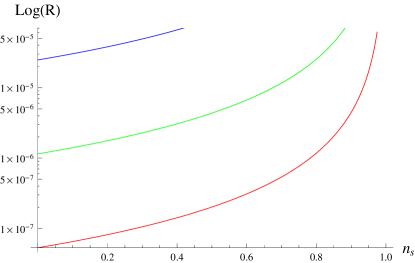
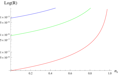
Figure 1: Variations in Log$(R)$ versus $n_{s}$: Left plot for $f^{\ast}=0.42,~{}\mu\approx 0.5,~{}n=1,~{}C_{\gamma}=70$, $C_{\psi}=10^{-6}$ (red), $C_{\psi}=10^{-5}$ (green), $C_{\psi}=10^{-4}$ (blue);    (Right) $f^{\ast}=0.37,~{}n=0,~{}C_{\psi}=10^{-9}$ (red), $C_{\psi}=10^{-7}$ (green), $C_{\psi}=10^{-6}$ (blue) during intermediate era.

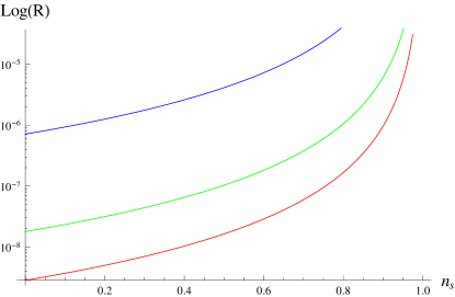
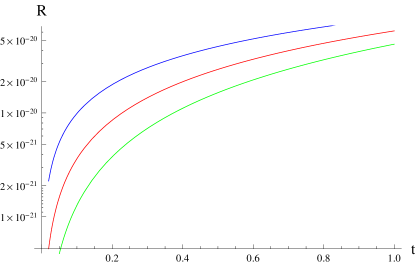
Figure 2: Log$(R)$ versus $n_{s}$ for $f^{\ast}=0.34,~{}\mu\approx 0.5,~{}n=-1,~{}C_{\gamma}=70$, $C_{\psi}=10^{-12}$ (red), $C_{\psi}=10^{-11}$ (green), $C_{\psi}=10^{-9}$ (blue) (Left). Variations in $R$ versus $t$ for $n=0$ (red), $n=-1$ (green), $n=1$ (blue) (Right).

The corresponding tensor perturbations are

$$P_{T}(k)=\frac{2\kappa}{9\pi^{2}}(\mu+2)^{2}H_{2}^{2}=\frac{2\kappa}{9\pi^{2}}(\mu+2)^{2}(A^{\ast}f^{\ast})^{2}\left(\frac{\psi}{\alpha_{0}}\right)^{\frac{4(f^{\ast}-1)}{f^{\ast}}}.$$ (20)

Combining Eqs.(15) and (20), the tensor to scalar ratio (in terms of $\psi,~{}N,~{}n_{s}$) becomes

$$r(k) = \alpha_{2}\psi^{\beta_{2}}=\alpha_{2}\left[\frac{24(1+2\mu)(1-f^{\ast})(1+f^{\ast}(N-1))}{\kappa(\mu+2)^{2}{f^{\ast}}^{2}}\right]$$ (21)

$$= \alpha_{2}\left[\frac{12(1+2\mu)(1-f^{\ast})(10-2n-f^{\ast}(17-5n))}{\kappa(\mu+2)^{2}{f^{\ast}}^{2}(4-n)(1-n_{s})}\right]^{\frac{\beta_{2}}{2}},$$

where

$$\alpha_{2}=\frac{2\kappa(\mu+2)^{2}(A^{\ast}f^{\ast})^{2}{\alpha_{0}}^{\frac{4(f^{\ast}-1)}{f^{\ast}}}}{9\pi^{2}\alpha_{1}},\quad\beta_{2}=\beta_{1}-\frac{4(1-f^{\ast})}{f^{\ast}}.$$

During weak dissipative regime, we have calculated constraint on the parameter $C_{\psi}$ using Eqs.(18), (19) and (21) in which $P_{R}=2.43\times 10^{-9}$. It is proved that in anisotropic model the dissipation coefficient $R$ evolutes during weak dissipative regime for these constraints (Figures 1 and 2). The range of parameter $C_{\psi}$ for three different values of $n$ and corresponding $f^{\ast}$ are given in Table 1. The parameter $f^{\ast}$ is obtained through Eq.(17) by fixing $N=70$ and $n_{s}=0.96$. Figures 3 and 4 show the dependence of $r$ on $n_{s}$ for specific values of the parameters. The left plot of Figure 3 (blue curve) shows that warm anisotropic model is well fitted with recent observations (WMAP9, Plank, BICEP2) for $C_{\psi}<10^{-4}$ during weak intermediate regime. We have also computed an upper bound, $C_{\psi}>10^{-6}$ that improves the compatibility of our model with recent observations. Planck data places stronger bound on $r,~{}n_{s}$ as compared to WMAP9 and BICEP2. Figure 3 (right panel) is plotted for $n=0$ and three different values of $C_{\psi}$ make the model well supported by the WMAP9, Planck as well as BICEP2 for $C_{\psi}<10^{-6}$. Similarly, for $n=-1$ (Figure 4), our model remains compatible with recent observations during $10^{-12}<C_{\psi}<10^{-9}$. We have found that the presence of anisotropic parameter $\mu$ leads to increase the values of $C_{\psi}$ as compared to FRW [26]. It is also noted that the value of $C_{\psi}$ decreases with the increase of $n$.

Table 1: Constraints on $C_{\psi}$ for different values of $n$

$n$	$f^{\ast}$	Constraint on $C_{\psi}$
1	0.42	$10^{-6}<C_{\psi}<10^{-4}$
0	0.37	$10^{-9}<C_{\psi}<10^{-6}$
-1	0.34	$10^{-12}<C_{\psi}<10^{-9}$

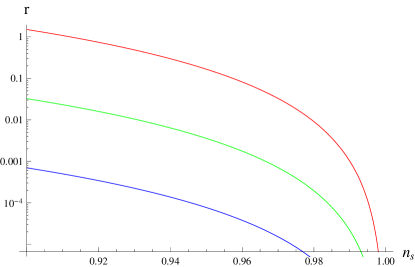
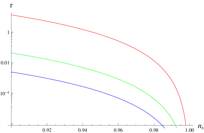
Figure 3: Plot of $r$ versus $n_{s}$: Left plot for $f^{\ast}=0.42,~{}\mu\approx 0.5,~{}n=1,~{}C_{\gamma}=70$, $C_{\psi}=10^{-6}$ (red), $C_{\psi}=10^{-5}$ (green), $C_{\psi}=10^{-4}$ (blue); (Right) $f^{\ast}=0.37,~{}n=0,~{}C_{\psi}=10^{-9}$ (red), $C_{\psi}=10^{-7}$ (green), $C_{\psi}=10^{-6}$ (blue) during intermediate era.

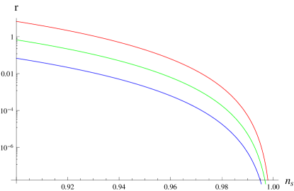
Figure 4: Plot of $r$ versus $n_{s}$ for $f^{\ast}=0.34,~{}\mu\approx 0.5,~{}n=-1,~{}C_{\gamma}=70$, $C_{\psi}=10^{-12}$ (red), $C_{\psi}=10^{-11}$ (green), $C_{\psi}=10^{-9}$ (blue).

3.2 Logamediate Era

During logamediate regime, the scale factor evolutes as [13]

$$Y(t)=Y_{0}\exp[A^{\ast}(\ln t)^{\lambda^{\ast}}].$$ (22)

Using this value, inflaton takes the form

$$\psi(t)-\psi(t_{0})=\left(\frac{2(1+2\mu)(A^{\ast}\lambda^{\ast})}{\kappa(\mu+2)}\right)^{\frac{1}{2}}\left(\frac{2}{\lambda^{\ast}+1}\right)(\ln t)^{\frac{\lambda^{\ast}+1}{2}}.$$ (23)

The cosmic time can be evaluated from the above equation as

$$t=\exp\left[-B_{0}\psi^{\nu}\right],$$

where $B_{0}=\left(\frac{\kappa(\mu+2)}{2\nu(1+2\mu)(A^{\ast}\lambda^{\ast})}\right)^{\frac{\nu}{2}},~{}\nu=\frac{2}{\lambda^{\ast}+1}$. Substituting the value of $t$, we obtain

$$H_{2}(\psi)=(A^{\ast}\lambda^{\ast}){B_{0}}^{(\lambda^{\ast}-1)}\psi^{\nu(\lambda^{\ast}-1)}\exp\left[-B_{0}\psi^{\nu}\right],$$

and $V(\psi)$ becomes

$$V(\psi)=V_{0}\psi^{\alpha_{3}}\exp\left[-\beta_{3}\psi^{\nu}\right],$$

where $V_{0}=\left(\frac{1+2\mu}{\kappa}\right)(A^{\ast}\lambda^{\ast})^{2}{B_{0}}^{2(\lambda^{\ast}-1)},~{}\alpha_{3}=2\nu(\lambda^{\ast}-1),~{}\beta_{3}=2B_{0}.$ Here the dissipation coefficient can be represented as

$$\Gamma(\psi)=C_{\psi}^{\frac{4}{4-n}}\left[\frac{3(1+2\mu)}{2\kappa C_{\gamma}(\mu+2)^{2}}\right]^{\frac{n}{4-n}}\psi^{\frac{4(1-n)}{4-n}}\exp\left[\left(\frac{n}{n-4}\right){B_{0}}^{\nu}\psi^{\nu}\right].$$

In weak dissipation regime, the decay rate $R=\frac{\Gamma}{(\mu+2)H_{2}}<1$ leads to constrain $C_{\psi}$ as given in Table 2. Figure 5 shows that the range $10^{-7}<C_{\psi}<10^{-3}$ for $n=1$ is compatible with weak dissipative regime. It is found that the evolution of $R$ versus $n_{s}$ for $n=0,-1$ also remains less than unity (graphs are not shown).

Table 2: Constraints on $C_{\psi}$ for different values of $n$

$n$	Constraint on $C_{\psi}$
1	$10^{-7}<C_{\psi}<10^{-3}$
0	$10^{-11}<C_{\psi}<10^{-7}$
-1	$10^{-13}<C_{\psi}<10^{-10}$

In logamediate inflation, the slow-roll parameters are

$$\epsilon = \left(\frac{3}{\mu+2}\right)(A^{\ast}\lambda^{\ast})^{-1}{B_{0}}^{-(\lambda^{\ast}-1)}\psi^{-\nu(\lambda^{\ast}-1)},$$

$$\eta = \left(\frac{3}{\mu+2}\right)(A^{\ast}\lambda^{\ast}{B_{0}}^{\lambda^{\ast}})^{-1}\psi^{-\nu\lambda^{\ast}}\left[2B_{0}\psi^{\nu}-(\nu-1)\right].$$

The range of inflaton is

$$\psi>\left[\left(\frac{\mu+2}{3}\right)(A^{\ast}\lambda^{\ast}){B_{0}}^{(\lambda^{\ast}-1)}\right]^{-\frac{1}{\nu(\lambda^{\ast}-1)}},$$

and the initial inflaton at $\epsilon=1$ is

$$\psi_{1}=\left[\left(\frac{\mu+2}{3}\right)(A^{\ast}\lambda^{\ast}){B_{0}}^{(\lambda^{\ast}-1)}\right]^{-\frac{1}{\nu(\lambda^{\ast}-1)}}.$$

The warm model has the following number of e-folds

$$N=\left(\frac{\mu+2}{3}\right)(A^{\ast}{B_{0}}^{\lambda^{\ast}})\left(\psi_{2}^{\nu\lambda^{\ast}}-\psi_{1}^{\nu\lambda^{\ast}}\right).$$

The inflaton dependent $P_{R}$ turns out to be

$$P_{R}(\psi) = \left(\frac{\kappa(\mu+2)^{4}}{6(1+2\mu)}\right)\left[\frac{3(1+2\mu)C_{\phi}}{2\kappa C_{\gamma}(\mu+2)^{2}}\right]^{\frac{1}{4-n}}(A^{\ast}\lambda^{\ast})^{2}{B_{0}}^{2(\lambda^{\ast}-1)}\psi^{(\alpha_{3}+\frac{1-n}{4-n})}$$ (24)

$$\times \exp\left[-\left(\frac{5-n}{4-n}\right)B_{0}\psi^{\nu}\right].$$

Another inflaton is defined by $\psi_{2}$ as

$$\psi_{2}=\left[\left(\frac{3}{\mu+2}\right){B_{0}}^{-\lambda^{\ast}}\left[\frac{N}{A^{\ast}}+\left(\left(\frac{\mu+2}{3}\right)(A^{\ast}\lambda^{\ast})^{\lambda^{\ast}}\right)^{-\frac{1}{\lambda^{\ast}-1}}\right]\right]^{\frac{1}{\nu\lambda^{\ast}}}.$$

Equation (24) can also be written in terms of $N$ using $\psi_{2}$ as

$$P_{R}(N) = \beta_{4}\left[\frac{N}{A^{\ast}}+\left(\left(\frac{\mu+2}{3}\right)(A^{\ast}\lambda^{\ast})^{\lambda^{\ast}}\right)^{-\frac{1}{\lambda^{\ast}-1}}\right]^{\frac{1}{\nu\lambda^{\ast}}(\alpha_{3}+\frac{1-n}{4-n})}\exp\left[\left(\frac{5-n}{n-4}\right)\right.$$ (25)

$$\times \left.\left(\frac{3}{\mu+2}\right)^{\frac{1}{\lambda^{\ast}}}\left[\frac{N}{A^{\ast}}+\left(\left(\frac{\mu+2}{3}\right)(A^{\ast}\lambda^{\ast})^{\lambda^{\ast}}\right)^{-\frac{1}{\lambda^{\ast}-1}}\right]^{\frac{1}{\lambda^{\ast}}}\right],$$

where

$$\beta_{4} = \left(\frac{\kappa(\mu+2)^{4}}{6(1+2\mu)}\right)\left[\frac{3(1+2\mu)C_{\psi}}{2\kappa C_{\gamma}(\mu+2)^{2}}\right]^{\frac{1}{4-n}}\left(\frac{3}{\mu+2}\right)^{\frac{1}{\nu\lambda^{\ast}}(\alpha_{3}+\frac{1-n}{4-n})}(A^{\ast}\lambda^{\ast})^{2}$$

$$\times {B_{0}}^{2(\lambda^{\ast}-1)-\frac{1}{\nu}(\alpha_{3}+\frac{1-n}{4-n})}.$$

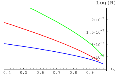
Figure 5: Log$(R)$ versus $n_{s}$ for $\mu\approx 0.5,~{}n=1,~{}C_{\gamma}=70,~{}A^{\ast}=6.65\times 10^{-3},~{}\lambda^{\ast}=6,~{}C_{\psi}=10^{-7}$ (red), $A^{\ast}=8.43\times 10^{-3},~{}\lambda^{\ast}=4.95,~{}C_{\psi}=10^{-5}$ (green) $A^{\ast}=2.88\times 10^{-2},~{}\lambda^{\ast}=4.36~{},C_{\psi}=10^{-3}$ (blue).

The spectral index for the present model becomes

$$n_{s}-1 = \left(\frac{3}{\mu+2}\right)\left[-\left(\frac{4(\lambda^{\ast}-1)}{A^{\ast}\lambda^{\ast}}+\frac{(1-n)(\lambda^{\ast}+1)}{2(A^{\ast}\lambda^{\ast})(4-n)}\right){B_{0}}^{-\lambda^{\ast}}\psi^{-\nu\lambda^{\ast}}\right.$$ (26)

$$+ \left.\left(\frac{5-n}{4-n}\right)\frac{{B_{0}}^{(1-\lambda^{\ast})}\psi^{\nu(1-\lambda^{\ast})}}{A^{\ast}\lambda^{\ast}}\right]$$

$$= -\left[\frac{N}{A^{\ast}}+\left(\left(\frac{\mu+2}{3}\right)(A^{\ast}\lambda^{\ast})^{\lambda^{\ast}}\right)^{-\frac{1}{\lambda^{\ast}-1}}\right]^{-1}\left(\frac{(1-n)(\lambda^{\ast}+1)}{2(A^{\ast}\lambda^{\ast})(4-n)}\right.$$

$$+ \left.\frac{4(\lambda^{\ast}-1)}{A^{\ast}\lambda^{\ast}}\right)+\frac{1}{A^{\ast}\lambda^{\ast}}\left(\frac{5-n}{4-n}\right)\left(\frac{3}{\mu+2}\right)^{\frac{1}{\lambda^{\ast}}+1}$$

$$\times \left[\frac{N}{A^{\ast}}+\left(\left(\frac{\mu+2}{3}\right)(A^{\ast}\lambda^{\ast})^{\lambda^{\ast}}\right)^{-\frac{1}{\lambda^{\ast}-1}}\right]^{\frac{1-\lambda^{\ast}}{\lambda^{\ast}}}.$$

The tensor power spectrum is

$$P_{T}(\psi)=\frac{2\kappa}{9\pi^{2}}(\mu+2)^{2}(A^{\ast}\lambda^{\ast})^{2}{B_{0}}^{2(\lambda^{\ast}-1)}\psi^{2\nu(\lambda^{\ast}-1)}\exp\left[-B_{0}\psi^{\nu}\right],$$

which leads to the following $r$ along with Eq.(25)

$$r(\psi) = \frac{4(1+2\mu)}{3\pi^{2}(\mu+2)^{2}}\left[\frac{2\kappa C_{\gamma}(\mu+2)^{2}}{3(1+2\mu)C_{\psi}}\right]^{\frac{1}{4-n}}\psi^{-\frac{1-n}{4-n}}\exp\left[\left(\frac{5-n}{4-n}-2\right)B_{0}\psi^{\nu}\right]$$ (27)

$$= \beta_{5}\left[\frac{N}{A^{\ast}}+\left(\left(\frac{\mu+2}{3}\right)(A^{\ast}\lambda^{\ast})^{\lambda^{\ast}}\right)^{-\frac{1}{\lambda^{\ast}-1}}\right]^{-\frac{(\lambda^{\ast}+1)(1-n)}{2\lambda^{\ast}(4-n)}}\exp\left[\left(\frac{5-n}{4-n}-2\right)\right.$$

$$\times \left.\left(\frac{3}{\mu+2}\right)^{\frac{1}{\lambda^{\ast}}}\left[\frac{N}{A^{\ast}}+\left(\left(\frac{\mu+2}{3}\right)(A^{\ast}\lambda^{\ast})^{\lambda^{\ast}}\right)^{-\frac{1}{\lambda^{\ast}-1}}\right]^{\frac{1}{\lambda^{\ast}}}\right].$$

where

$$\beta_{5}=\left(\frac{4(1+2\mu)}{3\pi^{2}(\mu+2)^{2}}\right)\left[\frac{2\kappa C_{\gamma}(\mu+2)^{2}}{3(1+2\mu)C_{\psi}}\right]^{\frac{1}{4-n}}\left(\frac{\mu+2}{3}\right)^{\frac{(\lambda^{\ast}+1)(1-n)}{2\lambda^{\ast}(4-n)}}{B_{0}}^{\frac{(\lambda^{\ast}+1)(1-n)}{2(4-n)}}.$$

Table 3: Constraints on $C_{\psi},~{}A^{\ast}$ and $\lambda^{\ast}$ for different values of $n$

$n$	$C_{\psi}$	$\lambda^{\ast}$	$A^{\ast}$
1	$10^{-7}$	6.00	$6.65\times 10^{-3}$
1	$10^{-5}$	4.95	$8.43\times 10^{-3}$
1	$10^{-3}$	4.36	$2.88\times 10^{-2}$
0	$10^{-11}$	4.00	$1.79\times 10^{-2}$
0	$10^{-9}$	4.35	$1.16\times 10^{-2}$
0	$10^{-7}$	4.57	$4.53\times 10^{-2}$
-1	$10^{-13}$	4.85	$3.15\times 10^{-2}$
-1	$10^{-12}$	3.95	$1.99\times 10^{-2}$
-1	$10^{-10}$	3.25	$8.33\times 10^{-2}$

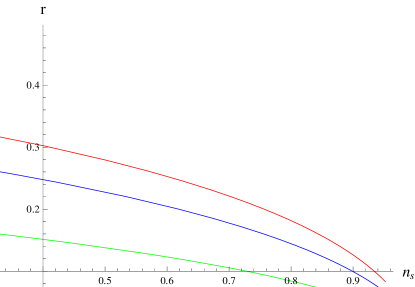
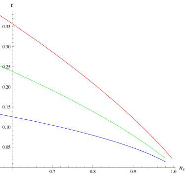
Figure 6: Plot of $r$ versus $n_{s}$: Left plot for $\mu\approx 0.5,~{}n=1,~{}C_{\gamma}=70$, $A^{\ast}=6.65\times 10^{-3},~{}\lambda^{\ast}=6,~{}C_{\psi}=10^{-7}$ (red), $A^{\ast}=8.43\times 10^{-3},~{}\lambda^{\ast}=4.95,~{}C_{\psi}=10^{-5}$ (green) $A^{\ast}=2.88\times 10^{-2},~{}\lambda^{\ast}=4.36~{},C_{\psi}=10^{-3}$ (blue); (Right) $A^{\ast}=1.79\times 10^{-2},~{}n=0,~{}\lambda^{\ast}=4,~{}C_{\psi}=10^{-11}$ (red), $A^{\ast}=1.16\times 10^{-2},~{}\lambda^{\ast}=4.35,~{}C_{\psi}=10^{-9}$ (green), $A^{\ast}=4.53\times 10^{-2},~{}\lambda^{\ast}=4.57,~{}C_{\psi}=10^{-7}$ (blue) during logamediate era.

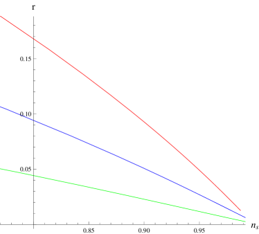
Figure 7: Plot of $r$ versus $n_{s}$ for $\mu\approx 0.5,~{}n=-1,~{}C_{\gamma}=70$, $A^{\ast}=3.15\times 10^{-2},~{}\lambda^{\ast}=4.85,~{}C_{\psi}=10^{-13}$ (red), $A^{\ast}=1.99\times 10^{-2},~{}\lambda^{\ast}=3.95,~{}C_{\psi}=10^{-12}$ (green), $A^{\ast}=8.33\times 10^{-2},~{}\lambda^{\ast}=3.25,~{}C_{\psi}=10^{-10}$ (blue).

In order to constrain the physical parameters used in warm logamediate model, we numerically solve Eqs.(25) and (26) for three different values of $n$. The values of the model parameters $A^{\ast}$ and $\lambda^{\ast}$ for particular $C_{\psi}$ are picked up from the defined range are given in Table 3. Figures 6 and 7 show two-dimensional marginalized constraints on the inflationary parameters $r$ and $n_{s}$ derived from recent data. These graphs are plotted for three different values of $A^{\ast},~{}\lambda^{\ast}$ and $C_{\psi}$. The left panel of Figure 6 proves that our anisotropic warm inflationary model is compatible with recent observations in the range $10^{-7}<C_{\psi}<10^{-3}$ as $n_{s}=0.96$ generates very weak bound $r<0.3$. Analogously, Figure 6 (right panel) verifies that the range $10^{-11}<C_{\psi}<10^{-7}$ remains well consistent with recent observations. Our anisotropic model satisfies the bounds of WMAP9, Planck and BICEP2 for $C_{\psi}<10^{-10}$ (Figure 7).

One of the characteristics of warm inflation is $T>H_{2}$, where $T$ is the temperature of thermal background of the radiation. Further, we assume that $T=T_{r}$, it is not a free parameter, we can restrict $T_{r}>5.47\times 10^{-5}$ using recent Planck data $n_{s}=0.96\pm 0.0073$ and an upper bound for $r<0.11$ at the pivot point $k_{0}=0.002Mpc^{-1}$. We have checked the condition of warm inflation ($T_{r}>H_{2}$) for our model. Figure 2 shows a restriction on $T_{r}=T$, i.e., $T_{r}>H$.

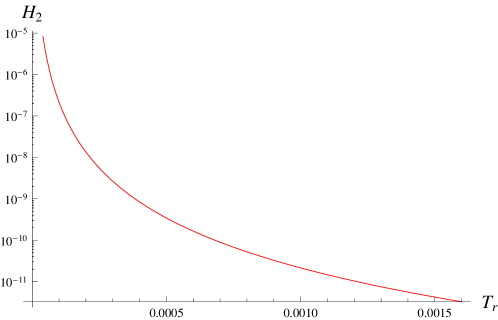
Figure 8: $H_{2}$ is plotted versus $T_{r}$.

4 Concluding Remarks

The idea of warm inflation is influenced by the friction term in the inflaton equation of motion. The magnitude of the damping term suggests the possibility that it could be the dominant effect prolonging inflation. In this paper, we study the possible realization of an expanding intermediate and logamediate scale factors in weak dissipative regime and analyze how these two types of inflation work with generalized form of the dissipation coefficient $(\Gamma=C_{\psi}\frac{T^{n}}{\psi^{n-1}})$. To this end, we have used the framework of homogeneous but anisotropic LRS BI universe model which is asymptotically equivalent to the standard FRW universe.

Recent data from the Planck satellite prove that large angle anomalies represent real feature of the CMB map of the universe. This result has a key importance since the small temperature anisotropies and large angle anomalies may be caused by some unknown mechanism or an anisotropic phase during the evolution of the universe. This statement is particularly interesting because it helps to modify the present model or to construct an alternative model to decode the effects of the early universe on the present day LSS without affecting the processes in the nucleosynthesis [27]. Scalar field leads to isotropisation, necessary for compatibility with standard cosmological models at late times, as well as inflation which accounts for structure formation. Anisotropic model provides bouncing solutions that corresponds to the late-time evolution which is driven to isotropy and spatial flatness. Inflationary models has ability to make a transition form early anisotropic phase to late-time isotropic evolution.

We have assumed that the universe is composed of standard scalar field and radiation. Under slow-roll approximation, we have found solutions of the first evolution equation (field equation) in weak dissipative regime. During intermediate and logamediate eras, the explicit expressions for inflaton $(\psi)$, corresponding effective potential $(V(\psi))$ and rate of dissipation $(R)$ are calculated. Moreover, we have evaluated perturbation parameters including slow-roll parameters $(\epsilon,~{}\eta)$ to find the more general conditions on the starting and ending conditions for the occurrence of inflationary era, scalar and tensor power spectra $(P_{R},~{}P_{T})$, scalar spectral index $(n_{s})$ and finally observational parameter of interest, i.e., tensor to scalar ratio $(r)$. In each case, we have constrained the model parameters $(A^{\ast},~{}f^{\ast},~{}\lambda^{\ast},~{}C_{\psi})$ by WMAP9, Planck and BICEP2 data for three particular values of $n=1,0,-1$.

In both regimes, we have proved that the values of the model parameters given in Tables 1-3 lead to $R<1$ as shown in Figures 1, 2 and 5. We conclude that theses constraints make our warm anisotropic inflationary model with generalized form of $\Gamma$ well supported by recent observations. The trajectories of $r-n_{s}$ plotted in both regimes are the verification of our results. The results of this paper deviate from FRW universe in the following way. During weak intermediate era, it is observed that due to the presence of anisotropic parameter, $\mu$, constraints on the important model parameter $C_{\psi}$ increase as compared to FRW universe. For example, in anisotropic universe (LRS BI), $n=1$ leads to $10^{-6}<C_{\psi}<10^{-4}$ while for isotropic universe (FRW), this is $10^{-9}<C_{\psi}<10^{-6}$. Further, it is observed that the value of $C_{\psi}$ decreases with the increase of $n$ due to anisotropic parameter. Since $C_{\psi}$ acts as coupling parameter, so its decreasing nature is well consistent with observations, i.e., coupling between two constituents of the universe must be decreasing with the cosmic evolution. This result has opposite effect as compared to isotropic universe. Similarly, in logamediate regime, we are successful in constraining $C_{\psi}<10^{-10}$ that leads to compatibility of the model with WMAP9, Planck as well as BICEP2. It is observed that the compatibility range of $C_{\psi}$ is less than FRW universe.

It is also found that compatibility of the model disturbs for too large values of the anisotropic parameter $\mu>10^{3}$. The case $n=3$ where ($\Gamma\propto\frac{T^{3}}{\phi^{2}}$) is discussed for strong dissipation regime during intermediate and logamediate regimes [20]. It is worth mentioning here that all the results reduce to the isotropic universe for $\mu=1$ [26] and $n=3$ leads to [32]. The work in strong dissipative regime and interpolation between weak and strong regimes is under process.

Acknowledgment

We would like to thank the Higher Education Commission, Islamabad, Pakistan for its financial support through the Indigenous Ph.D. Fellowship for 5000 Scholars Phase-II, Batch-I.

References

- [1] Larson, D. et al.: Astrophys. J. Suppl. 192(2011)16; Komatsu, E. et al.: Astrophys. J. Suppl. 192(2011)18.
- [2] Kolb, E.W. and Turner, M.S.: The Early Universe (Addison-Wesley, 1990).
- [3] Bassett, B.A., Tsujikawa, S. and Wands, D.: Rev. Mod. Phys. 78(2006)537.
- [4] Bartrum, S. et al.: Phys. Lett. B 732(2014)116; Bastero-Gil, M., Berera, A., Ramos, R.O. and Rosa, J.G.: J. Cosmol. Astropart. Phys. 1410(2014)053.
- [5] Berera, A.: Phys. Rev. Lett. 75(1995)3218; Phys. Rev. D 55(1997)3346.
- [6] Moss, I.G.: Phys. Lett. B 154(1985)120; Berera, A.: Nucl. Phys. B 585(2000)666; Hall, L.M.H., Moss, I.G. and Berera, A.: Phys. Rev. D 69(2004)083525.
- [7] Yokoyama, J. and Linde, A.: Phys. Rev. D 60(1999)083509; Berera, A., Gleiser, M. and Ramos, R.O.: Phys. Rev. D 58(1998)123508.
- [8] Bastero-Gil, M., Berera, A. and Ramos, R.O.: J. Cosmol. Astropart. Phys. 1109(2011)033; Bastero-Gil, M., Berera, A., Ramos, R.O. and Rosa, J.G.: J. Cosmol. Astropart. Phys. 1301(2013)016.
- [9] Berera, A. and Ramos, R.O.: Phys. Rev. D 63(2001)103509.
- [10] Lucchin, F. and Matarrese, S.: Phys. Rev. D 32(1985)1316 .
- [11] Guth, A.: Phys. Rev. D 23(1981)347 .
- [12] Barrow, J.D.: Phys. Lett. B 235(1990)40; Barrow, J.D. and Saich, P.: Phys. Lett. B 249(1990)406; Muslimov, A.: Class. Quantum Grav. 7(1990)231; Rendall, A.D.: Class. Quantum Grav. 22(2005)1655.
- [13] Barrow, J.D. and Nunes, N.J.: Phys. Rev. D 76(2007)043501 .
- [14] Sanyal, A.K.: Phys. Lett. B 645(2007)1.
- [15] Barrow, J.D.: Class. Quantum Grav. 13(1996)2965.
- [16] Barrow, J.D. and Liddle, A.R.: Phys. Rev. D 47(1993)R5219; Starobinsky, A.A.: J. Exp. Theor. Phys. Lett. 82(2005)169; del Campo, S., Herrera, R., Saavedra, J., Campuzano, C. and Rojas, E.: Phys. Rev. D 80(2009)123531; Herrera, R. and Videla, N.: Eur. Phys. J. C 67(2010)499; Herrera, R., Olivares, M. and Videla, N.: Eur. Phys. J. C 73(2013)2295.
- [17] Kinney, W.H., Kolb, E.W., Melchiorri, A. and Riotto, A.: Phys. Rev. D 74(2006)023502; Barrow, J.D., Liddle, A.R. and Pahud, C.: Phys. Rev. D 74(2006)127305.
- [18] Ade, P.A.R. et al.: arXiv:1403.3985; arXiv:1403.4302.
- [19] Setare, M.R. and Kamali, V.: Phys. Lett. B 726(2013)56; Gen. Relativ. Gravit. 46(2014)1642.
- [20] Sharif, M. and Saleem, R.: Eur. Phys. J. C 74(2014)2738; Astropart. Phys. 62(2015)100.
- [21] del Campo, S. and Herrera, R.: Phys. Lett. B 660(2008)282; ibid. 665(2008)100.
- [22] Herrera, R., Olivares, M. and Videla, N.: Eur. Phys. J. C 73(2013)2295.
- [23] Sharif, M. and Saleem, R.: Eur. Phys. J. C 74(2014)2943; J. Cosmol. Astropart. Phys. 12(2014)038.
- [24] Setare, M.R. and Kamali, V.: Gen. Relativ. Gravit. 46(2014)1698; arXiv:1312.2832.
- [25] Sharif, M. and Saleem, R.: Astropart. Phys. 62(2015)241.
- [26] Herrera, R., Olivares, M. and Videla, N.: Phys. Rev. D 88(2013)063535; Int. J. Mod. Phys. D 23(2014)1450080.
- [27] Russell, E., Kilinc, C.B. and Pashaev, O.K.: Mon. Not. R. Astron. Soc. 442(2014)2331.
- [28] Planck Collaboration Ade, P.A.R., Aghanim, N., Armitage-Caplan, C., Arnaud, M., Ashdown, M., Atrio-Barandela, F., Aumont, J., Baccigalupi, C., Banday, A.J., et al.: arXiv:1303.5075.
- [29] Martinez-Gonzalez, E. and Sanz, J.L.: Astron. Astrophys. 300(1995)346.
- [30] Zhang, Y.: J. Cosmol. Astropart. Phys. 03(2009)030; Bastero-Gil, M., Berera, A. and Ramos, R.O.: J. Cosmol. Astropart. Phys. 07(2011)030.
- [31] Moss, G. and Xiong, C.: arXiv:hep-ph/0603266; Berera, A., Moss, I.G. and Ramos, R.O.: Rept. Prog. Phys. 72(2009)026901; Bastero-Gil, M., Berera, A. and Ramos, R.O.: J. Cosmol. Astropart. Phys. 09(2011)033; Cerezo, R. and Rosa, J.G.: J. High Energy Phys. 01(2013)024.
- [32] del Campo, S. and Herrera, R.: J. Cosmol. Astropart. Phys. 04(2009)005; Herrera, R. and Olivares, M.: Int. J. Mod. Phys. D 21(2012)1250047.
- [33] Hwang, J.C. and Noh, H.: Phys. Rev. D 66(2002)084009.
- [34] Freese, K., Frieman, J.A. and Olinto, A.V.: Phys. Rev. Lett. 65(1990)3233.
- [35] Bastero-Gil, M., Berera, A., Moss, I.G. and Ramos, R.O.: arXiv:1401.1149.