A note on the equivalence of Lagrangian and Hamiltonian formulations at post-Newtonian approximations

Abstract

It was claimed recently that a low order post-Newtonian (PN) Lagrangian formulation, which corresponds to the Euler-Lagrange equations up to an infinite PN order, can be identical to a PN Hamiltonian formulation at the infinite order from a theoretical point of view. This result is difficult to check because in most cases one does not know what both the Euler-Lagrange equations and the equivalent Hamiltonian are at the infinite order. However, no difficulty exists for a special 1PN Lagrangian formulation of relativistic circular restricted three-body problem, where both the Euler-Lagrange equations and the equivalent Hamiltonian not only are expanded to all PN orders but also have converged functions. Consequently, the analytical evidence supports this claim. As far as numerical evidences are concerned, the Hamiltonian equivalent to the Euler-Lagrange equations for the lower order Lagrangian requires that they both be only at higher enough finite orders.

I Introduction

In classical mechanics, Lagrangian and Hamiltonian formulations are completely the same description of a dynamical system. Usually more attention to the Hamiltonian formulation is paid because it has properties of a canonical system.

In post-Newtonian (PN) mechanics of general relativity, the two formulations are still adopted. Are they completely equivalent? Ten years ago two independent groups [1,2] answered this question. They proved the complete physical equivalence of the third-order post-Newtonian (3PN) Arnowitt-Deser-Misner (ADM) coordinate Hamiltonian approach to and the 3PN harmonic coordinate Lagrangian approach to the dynamics of spinless compact binaries. This result was recently extended to the inclusion of the next-to-next-to-leading order (4PN) spin-spin coupling [3].

However, there are two different claims on the chaotic behavior of compact binaries with one body spinning and spin effects restricted to spin-orbit (1.5PN) coupling. That is, the 2PN harmonic coordinate Lagrangian dynamics allow the onset of chaos [4], but the 2PN ADM Hamiltonian dynamics are integrable, regular and non-chaotic [5,6].

An explanation to the opposite results was given in [7]. In fact, the 2PN Hamiltonian and Lagrangian formulations are not exactly equal but are only approximately related. As its detailed account, the equations of motion for the Lagrangian formulation use lower-order terms as approximations to higher-order acceleration terms in the Euler-Lagrange equations, while these approximations do not occur in the equations of motion for the Hamiltonian formulation. It is natural that the Lagrangian has approximate constants of motion but the Hamiltonian contains exact ones. These facts were regarded as the essential point for the two formulations having different dynamics. In this sense, the two claims that seem to be explicitly conflicting were thought to be correct.

Recently, the authors of [8] revisited the equivalence between the Hamiltonian and Lagrangian formulations at PN approximations. They found that the two formulations at the same PN order are nonequivalent in general and have differences. Three simple examples of PN Lagrangian formulations, including a relativistic restricted three-body problem with the 1PN contribution from the circular motion of two primary objects, a spinning compact binary system with the Newtonian term and the leading-order spin-orbit coupling [8] and a binary system of the Newtonian term and the leading-order spin-orbit and spin-spin couplings [9], were used to show that the differences are not mainly due to the Lagrangian having the approximate Euler-Lagrange equations and the approximate constants of motion but come from truncation of higher-order PN terms between the two formulations transformed. An important result from the logic is that an equivalent Hamiltonian of a lower-order Lagrangian is usually at an infinite order from a theoretical point of view or at a higher enough order from numerical computations. Based on this, the integrability or non-integrability of the Lagrangian can be known by that of the Hamiltonian. More recently, chaos in comparable mass compact binary systems with one body spinning was completely ruled out [10]. The reason is that a completely canonical higher-order Hamiltonian, which is equivalent to a lower-order conservative Lagrangian and holds four integrals of the total energy and the total angular momentum in an eight-dimensional phase space, is typically integrable [11]. This result is useful to clarify the doubt on the absence of chaos in the 2PN ADM Hamiltonian approach [5,6] and the presence of chaos in the 2PN harmonic coordinate Lagrangian formulation [4]. As a point to illustrate, two other doubts about different chaotic indicators resulting in different dynamical behaviours of spinning compact binaries among references [12-15] and different descriptions of chaotic parameter spaces and chaotic regions between two articles [4,16] have been clarified in [17-19].

It is worth noting that the logic result on the equivalence of the PN Hamiltonian and Lagrangian approaches at different orders is not easy to check because the exactly equivalent Hamiltonian of the Lagrangian is generally expressed as an infinite series whose convergence is unknown clearly in most cases. To provide enough evidence for supporting this result, we select a part of the 1PN Lagrangian formulation of relativistic circular restricted three-body problem [20], where the Euler-Lagrange equations can be described by a converged Taylor series and the equivalent Hamiltonian can also be written as another converged Taylor series. For our purpose, the Hamiltonian is derived from the Lagrangian in Sect. 2. Then in Sect. 3 numerical methods are used to evaluate whether various PN order Hamiltonians and the 1PN Lagrangian with various PN order Euler-Lagrange equations are equivalent. Finally, the main results are concluded in Sect. 4.

II Post-Newtonian approximations

As in classical mechanics, a Lagrangian formulation $L(\mathbf{\dot{r}},\mathbf{r})$ and its Hamiltonian formulation $H(\mathbf{p},\mathbf{r})$ satisfy the Legendre transformation in PN mechanics. This transformation is written as

$$H(\mathbf{p},\mathbf{r})=\mathbf{p}\cdot\mathbf{\dot{r}}-L(\mathbf{\dot{r}},\mathbf{r}).$$ (1)

Here $\mathbf{r}$ and $\mathbf{\dot{r}}$ are coordinate and velocity, respectively. Canonical momentum is

$$\mathbf{p}=\frac{\partial L(\mathbf{\dot{r}},\mathbf{r})}{\partial\mathbf{\dot{r}}}.$$ (2)

Taking a special PN circular restricted three-body problem as an example, now we derive the Hamiltonian from the Lagrangian in detail.

II.1 Lagrangian formulation

The circular restricted three-body problem means the motion of a third body (i.e. a small particle of negligible mass) moving around two masses $m_{1}$ and $m_{2}$ ($m_{1}\geq m_{2}$). The two masses move in circular, coplanar orbits about their common center of mass, and have a constant separation $a$ and the same angular velocity. They exert a gravitational force on the particle but the third body does not affect the motion of the two massive bodies. Taking the unit of mass $G(m_{1}+m_{2})=1$, we have the two masses $\mu_{1}=m_{1}/(m_{1}+m_{2})$ and $\mu_{2}=m_{2}/(m_{1}+m_{2})$. The unit of length requires that the constant separation of the two bodies should be unity. The common mean motion, the Newtonian angular velocity $\omega_{0}$, of the two primaries is also unity. In these unit systems, the two bodies are stationary at points $O_{1}(x_{1},0)$ and $O_{2}(x_{2},0)$ with $x_{1}=-\mu_{2}$ and $x_{2}=\mu_{1}$ in the rotating reference frame. State variables $(\mathbf{\dot{r}},\mathbf{r})$ of the third body satisfy the following Lagrangian formulation

$$L = L_{0}+\frac{1}{c^{2}}L_{1}+\frac{1}{c^{2}}L_{2},$$ (3)

$$L_{0} = \frac{1}{2}(\dot{x}^{2}+\dot{y}^{2}+x^{2}+y^{2})+x\dot{y}-\dot{x}y+U,$$ (4)

$$L_{1} = \omega_{1}(x\dot{y}-\dot{x}y+x^{2}+y^{2}),$$ (5)

$$L_{2}=\frac{3}{2a}U[\dot{x}^{2}+\dot{y}^{2}+x^{2}+y^{2}+2(x\dot{y}-\dot{x}y)].$$ (6)

In the above equations, the related notations are specified as follows. $U$ is of the form

$$U=\frac{\mu_{1}}{r_{1}}+\frac{\mu_{2}}{r_{2}},$$ (7)

where the distances from body 3 to bodies 1 and 2 are

$$r_{1} = \sqrt{(x-x_{1})^{2}+y^{2}},$$

$$r_{2} = \sqrt{(x-x_{2})^{2}+y^{2}}.$$

$L_{0}$ stands for the Newtonian circular restricted three-body problem. $L_{1}$ is a 1PN contribution due to the relativistic effect to the circular motions of the two primaries. $L_{2}$ is also a 1PN contribution from the relativistic effect to the third body, and is only a part of that in [20] for our purpose. $\omega_{1}$ is the 1PN effect with respect to the angular velocity $\omega_{0}$ of the primaries and is given by

$$\omega_{1}=(\mu_{1}\mu_{2}-3)/(2a).$$ (8)

In fact, the separation $a$ is a mark of $L_{1}$ and $L_{2}$ as the 1PN effects when the velocity of light, $c$, is taken as one geometric unit in later numerical computations.

The Lagrangian (3) is a function of velocities and coordinates, therefore, its equations of motion are the ordinary Euler-Lagrange equations:

$$\frac{d}{dt}(\frac{\partial L}{\partial\dot{x}})=\frac{\partial L}{\partial x},~{}~{}~{}~{}~{}~{}~{}~{}\frac{d}{dt}(\frac{\partial L}{\partial\dot{y}})=\frac{\partial L}{\partial y}.$$ (9)

Since the momenta $p_{x}=\partial L/\partial\dot{x}$ and $p_{y}=\partial L/\partial\dot{y}$ of the forms

$$p_{x} = \dot{x}-(1+\frac{\omega_{1}}{c^{2}})y+\frac{3U}{ac^{2}}(\dot{x}-y),$$ (10)

$$p_{y} = \dot{y}+(1+\frac{\omega_{1}}{c^{2}})x+\frac{3U}{ac^{2}}(\dot{y}+x)$$ (11)

are linear functions of velocities $\dot{x}$ and $\dot{y}$, accelerations can be solved exactly from Eq. (9). They have detailed expressions:

$$\ddot{x} = \frac{X_{0}+X_{1}/c^{2}}{1+3U/(ac^{2})},$$ (12)

$$\ddot{y} = \frac{Y_{0}+Y_{1}/c^{2}}{1+3U/(ac^{2})}.$$ (13)

The Newtonian terms $X_{0}$ and $Y_{0}$ and the 1PN terms $X_{1}$ and $Y_{1}$ are

$$X_{0} = x+2\dot{y}+U_{x},$$ (14)

$$Y_{0} = y-2\dot{x}+U_{y},$$ (15)

$$X_{1} = 2\omega_{1}(x+\dot{y})+\frac{U_{x}}{U}L_{2}+\frac{3}{a}[U(x+2\dot{y})$$ (16)

$$-(\dot{x}U_{x}+\dot{y}U_{y})(\dot{x}-y)],$$

$$Y_{1} = 2\omega_{1}(y-\dot{x})+\frac{U_{y}}{U}L_{2}+\frac{3}{a}[U(y-2\dot{x})$$ (17)

$$-(\dot{x}U_{x}+\dot{y}U_{y})(x+\dot{y})],$$

where $U_{x}=\partial U/\partial x$ and $U_{y}=\partial U/\partial y$. Considering that $\delta=3U/a$ is at the 1PN level, Eqs. (12) and (13) have the Taylor expansions

$$\ddot{x} \approx X_{0}[\sum\limits_{i=0}^{k}(-1)^{i}(\frac{\delta}{c^{2}})^{i}]+\frac{X_{1}}{c^{2}}[\sum\limits_{j=0}^{k-1}(-1)^{j}(\frac{\delta}{c^{2}})^{j}],$$ (18)

$$\ddot{y} \approx Y_{0}[\sum\limits_{i=0}^{k}(-1)^{i}(\frac{\delta}{c^{2}})^{i}]+\frac{Y_{1}}{c^{2}}[\sum\limits_{j=0}^{k-1}(-1)^{j}(\frac{\delta}{c^{2}})^{j}].$$ (19)

They are the Euler-Lagrange equations with PN approximations to an order $k\geq 1$, labeled as $EL_{k}$. As a point to illustrate, the case of $k=0$ with $X_{1}=Y_{1}=0$ corresponds to the Newtonian Euler-Lagrange equations, marked as $EL_{0}$. From a theoretical viewpoint, as $k\rightarrow\infty$, $EL_{k}$ is strictly equivalent to $EL$ given by Eqs. (12) and (13), namely, $EL_{\infty}\equiv EL$. Note that for the generic case in [8], the momenta are highly nonlinear functions of velocities, so no exact equations of motion similar to Eqs. (12) and (13) but approximate equations of motion can be obtained from the Euler-Lagrange equations (9). This means that we do not know what the PN approximations like Eqs. (18) and (19) are converged as $k\rightarrow\infty$.

II.2 Hamiltonian formulations

The velocities $\dot{x}$ and $\dot{y}$ obtained from Eqs. (10) and (11) are expressed as

$$\dot{x} = \frac{p_{x}}{1+\delta/c^{2}}+(1+\frac{\omega_{1}}{c^{2}}){y},$$ (20)

$$\dot{y} = \frac{p_{y}}{1+\delta/c^{2}}-(1+\frac{\omega_{1}}{c^{2}}){x}.$$ (21)

Of course, they can be expanded to the $k$th order

$$\dot{x} \approx p_{x}[\sum\limits_{i=0}^{k}(-1)^{i}(\frac{\delta}{c^{2}})^{i}]+(1+\frac{\omega_{1}}{c^{2}}){y},$$ (22)

$$\dot{y} \approx p_{y}[\sum\limits_{i=0}^{k}(-1)^{i}(\frac{\delta}{c^{2}})^{i}]-(1+\frac{\omega_{1}}{c^{2}}){x}.$$ (23)

As mentioned above, Eqs. (22) and (23) are exactly identical to Eqs. (20) and (21) when $k\rightarrow\infty$.

In light of Eqs. (1), (20) and (21), we have the following Hamiltonian

$$H = \frac{1}{2(1+\delta/c^{2})}(p^{2}_{x}+p^{2}_{y})+(1+\frac{\omega_{1}}{c^{2}})(yp_{x}-xp_{y})$$ (24)

$$-U.$$

Its Taylor series at the $k$th order is of the form

$$H_{k} = \frac{1}{2}(p^{2}_{x}+p^{2}_{y})\sum\limits_{i=0}^{k}(-1)^{i}(\frac{\delta}{c^{2}})^{i}+(1+\frac{\omega_{1}}{c^{2}})(yp_{x}-xp_{y})$$ (25)

$$-U.$$

It is clear that $H_{0}$ with $\omega_{1}=0$ is the Newtonian Hamiltonian formulation, and can be expressed in terms of the Jacobian constant $C_{J}$ as $H_{0}\equiv-C_{J}/2$. Additionally, $H_{k}$ is closer and closer to $H$ as $k$ gets larger. Without doubt, the exact equivalence between $H$ and $H_{k}$ should be $H_{\infty}\equiv H$. Of course, what $H_{k}$ is converged as $k\rightarrow\infty$ is still unknown for the general case in [8].

It should be emphasized that $EL_{k}$ is the $k$th order PN approximation to the Euler-Lagrange equations $EL$ that is exactly derived from the 1PN Lagrangian $L$, and $H_{k}$ is the $k$th order PN approximation to the Hamiltonian $H$. Because of the exact equivalence between $EL$ and $H$, $EL_{k}$ is the $k$th order PN approximation to the Hamiltonian $H$, and $H_{k}$ is the $k$th order PN approximation to the Euler-Lagrange equations $EL$. Additionally, $EL_{\infty}$ and $H_{\infty}$ are exactly equivalent, i.e., $EL_{\infty}\equiv EL\Leftrightarrow H\equiv H_{\infty}$. However, it would be up to a certain higher enough finite order $k$ rather than up to the infinite order $k$ that the equivalence $EL_{k}\Leftrightarrow H_{k}$ can be checked by numerical methods. See the following numerical investigations for more details.

III Numerical investigations

Besides the above analytical method, a numerical method is used to estimate whether these PN approaches have constants of motion and what the accuracy of the constants is. Above all, we are interested in knowing whether these PN approaches are equivalent.

III.1 Energy errors

An eighth- and ninth-order Runge–Kutta–Fehlberg algorithm of variable time-steps is used to solve each of the above Euler-Lagrange equations $EL_{k}$ and Hamiltonians $H_{k}$. Parameters and initial conditions are $C_{J}=3.12$, $\mu_{2}=0.001$, $x=y=0.55$ and $\dot{x}=0$. Note that the initial positive value of $\dot{y}$ is given by the Jacobian constant. This orbit in the Newtonian problem $L_{0}$ is a Kolmogorov-Arnold-Moser (KAM) torus on the Poincaré section $y=0$ with $\dot{y}>0$ in Fig. 1(a), therefore, it is regular and non-chaotic. The integrator can give errors of the energy $H_{0}$ for the Lagrangian $L_{0}$ in the magnitude of order $10^{-13}$ or so. The long-term accumulation of energy errors is explicitly present in Fig. 1(b) because the integration scheme itself yields an artificial excitation or damping. If this accumulation is neglected, the energy should be constant. This shows that the energy $H_{0}$ is actually an integral of the Lagrangian $L_{0}$. However, the existence of this excitation or damping does not make the numerical results unreliable during the integration time of $10^{5}$ due to such a high numerical accuracy. In this sense, not only the integrator does not necessarily use manifold correction methods [21-23], but also it gives true qualitative results as a symplectic integration algorithm [24-27] does.

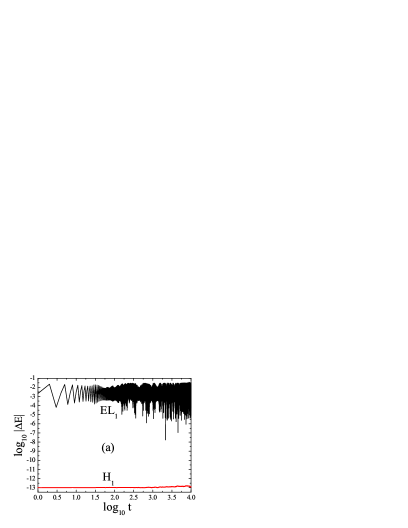
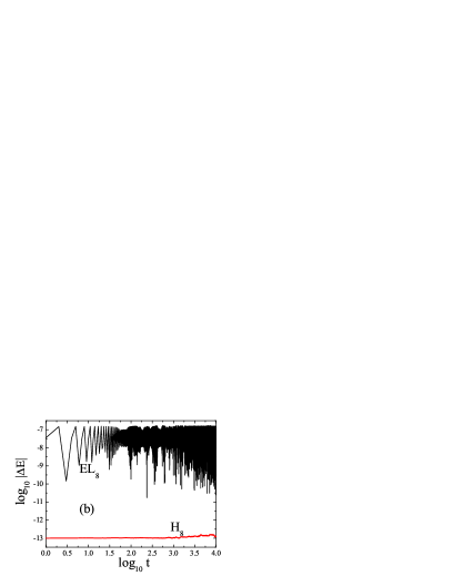
Figure 2: (color online) Energy errors $\Delta E$ for the related PN Lagrangian formulations with the separation $a=31$. Here are some examples to illustrate notations. For $EL_{1}$, $\Delta E=H_{1}-\tilde{H}_{1}$, where $\tilde{H}_{1}$ is the initial energy and the energy $H_{1}$ at time $t$ is obtained from the solution of $EL_{1}$. For $H_{1}$, $\Delta E=H_{1}-\tilde{H}_{1}$, where the energy $H_{1}$ at time $t$ is obtained from the solution of $H_{1}$. For $EL$, $\Delta E=H-\tilde{H}$, where $\tilde{H}$ is the initial energy and the energy $H$ at time $t$ is obtained from the solution of $EL$.

When the PN terms $L_{1}$ and $L_{2}$ are included, what about the accuracy of energy integrals given by the related PN approximations? Let us answer this question. Taking the separation between the primaries, $a=31$, we plot Fig. 2(a) in which the errors of energies of the 1PN Euler-Lagrange equations $EL_{1}$ and Hamiltonian $H_{1}$ are shown. It is worth noting that the error of energy is estimated by means of $\Delta=H_{1}-\tilde{H}_{1}$, where $H_{1}$ is regarded as the energy of $EL_{1}$ at time $t$ and $\tilde{H}_{1}$ is the initial energy. Obviously, the error for $EL_{1}$ is larger in about 10 orders of magnitude than that for $H_{1}$. This result should be very reasonable because differences between $EL_{1}$ and $H_{1}$ exist explicitly but the canonical equations are exactly given by the 1PN Hamiltonian $H_{1}$, as shown in the above analytical discussions. In other words, the difference between $EL_{1}$ and $H_{1}$ is at 1PN level. Of course, the higher the order $k$ gets, the smaller the difference between $EL_{k}$ and $H_{k}$ becomes. This is why we can see from Figs. 2(a) and 2(b) that the error of the 8PN Euler-Lagrange equations $EL_{8}$ and Hamiltonian $H_{8}$ is typically smaller than that of the 1PN Euler-Lagrange equations $EL_{1}$ and Hamiltonian $H_{1}$. Without doubt, $EL$ and $H$ should be the same in the energy accuracy if no roundoff errors exist in Fig. 2(c).

In addition to evaluating the accuracy of energy integrals of these PN approaches, evaluating the quality of these PN approaches to the Euler-Lagrange equations $EL$ or the Hamiltonian $H$ is also necessary from qualitative and quantitative numerical comparisons. See the following demonstrations for more information.

III.2 Qualitative comparisons

Besides the method of Poincaré sections, the method of Lyapunov exponents is often used to detect chaos from order. It relates to the description of average exponential deviation of two nearby orbits. Based on the two-particle method [28], the largest Lyapunov exponent is calculated by

$$\lambda=\lim_{t\rightarrow\infty}\frac{1}{t}\ln\frac{d(t)}{d(0)},$$ (26)

where $d(0)$ and $d(t)$ are distances between the two nearby trajectories at times 0 and $t$, respectively. A globally stable orbit is said to be regular if $\lambda=0$ but chaotic if $\lambda>0$. Generally speaking, it costs a long enough time to obtain a stabilizing value of $\lambda$ from the limit. Instead, a quicker method to find chaos is a fast Lyapunov indicator [29,30], defined as

$$FLI=\log_{10}\frac{d(t)}{d(0)}.$$ (27)

The globally stable orbit is chaotic if this indicator increases exponentially with time $\log_{10}t$ but ordered if this indicator grows polynomially.

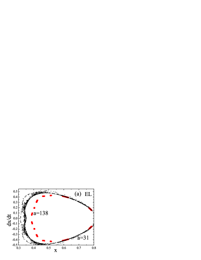
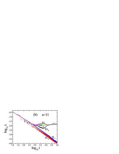
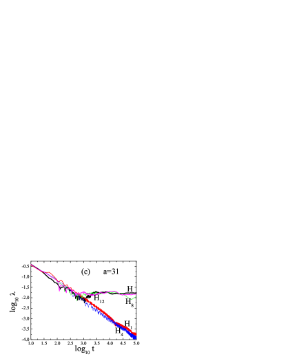
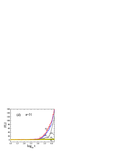
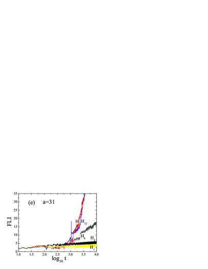
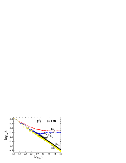
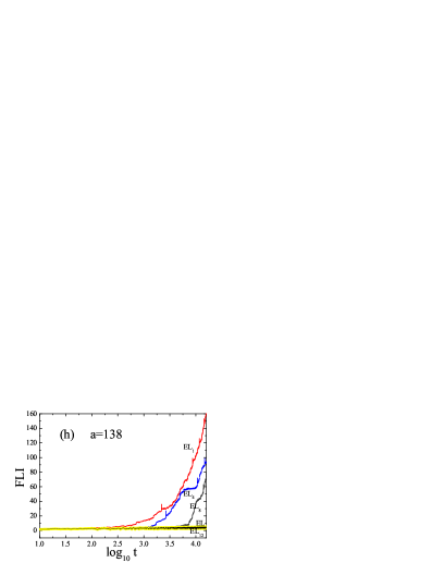
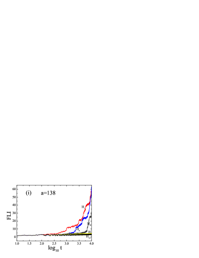
Figure 3: (color online) (a) Poincaré section for the orbit of Fig. 1 in the PN Euler-Lagrange equations $EL$ with the separation $a=31$ or $a=138$. Panels (b), (c), (f) and (g) relate to Lyapunov exponents $\lambda$, and panels (d), (e), (h) and (i) deal with FLIs.

It can be seen clearly from the Poincaré section of Fig. 3(a) that the dynamics of $EL$ or $H$ in Fig. 2(c) is chaotic. This result is supported by the Lyapunov exponents in Figs. 3(b) and 3(c) and the FLIs in Fig. 3(d) and 3(e). What about the dynamics of these various PN approximations? The key to this question can be found in Figs. 3(b)-3(e). Here are the related details. As shown in Fig. 3(b), lower order PN approximations to the Euler-Lagrange equations $EL$, such as the 1PN Euler-Lagrange equations $EL_{1}$ and the 4PN Euler-Lagrange equations $EL_{4}$, are so poorer that their dynamics are regular, and are completely unlike the chaotic dynamics of $EL$. With increase of the PN order $k$, higher order PN approximations to the Euler-Lagrange equations $EL$ become better and better. For example, the 8PN Euler-Lagrange equations $EL_{8}$ allows the onset of chaos, as $EL$ does. Seen particularly from the evolution curve on the Lyapunov exponent and time, the 12PN Euler-Lagrange equations $EL_{12}$ seems to be very closer to $EL$. These results are also suitable for the PN Hamiltonian approximations to the Hamiltonian $H$ in Fig. 3(c). When the Lyapunov exponents in Figs. 3(b) and 3(c) are replaced with the FLIs in Figs. 3(d) and 3(e), similar results can be given.

When the separation $a=138$ is instead of $a=31$ in Fig. 3(a), an ordered KAM torus occurs. That means that the $EL$ dynamics is regular and non-chaotic. In Figs 3(f)-3(i), lower order PN approximations such as $EL_{8}$ (or $H_{8}$) have chaotic behaviors, but higher order PN approximations such as $EL_{12}$ (or $H_{12}$) have regular behaviors.

In short, the above numerical simulations seem to tell us that the Euler-Lagrange equations (or the Hamiltonian approaches) at higher enough PN orders have the same dynamics as the Euler-Lagrange equations $EL$ (or the Hamiltonian $H$). There is a question of whether these results depend on the separation $a$. To answer it, we fix the above-mentioned orbit but let $a$ begin at 10 and end at 250 in increments of 1. For each given value of $a$, the FLI is obtained after integration time $t=3500$. In this way, we have dependence of FLIs on the separations $a$ in several PN Lagrangian and Hamiltonian approaches, plotted in Fig. 4. Here 5.5 is referred as a threshold value of FLI for distinguishing between the regular and chaotic cases at this time. That is to say, an orbit is chaotic when its FLI is larger than threshold but ordered when its FLI is smaller than threshold. In light of this, we do not find that there are dramatic dynamical differences between the Euler-Lagrange equations $EL$ (or the Hamiltonian $H$) and the various PN approximations such as the 1PN Hamiltonian $H_{1}$ and the 1PN Euler-Lagrange equations $EL_{1}$. However, it is clearly shown in Table 1 that regular and chaotic domains of smaller separations $a$ in the lowest PN approaches $EL_{1}$ and $H_{1}$ are explicitly different from those in $EL$ or $H$. As claimed above, this result is of course expected. When the order $k$ gets higher and higher, $EL_{k}$ and $H_{k}$ have smaller and smaller dynamical differences compared with $EL$ or $H$. Two points are worth noting. First, the same order PN approaches like $EL_{12}$ and $H_{12}$ (but unlike $EL$ and $H$) are incompletely equivalent in the dynamical behaviors for smaller values of $a$. Second, all the PN approaches $EL_{1}$, $H_{1}$, $EL_{12}$, $H_{12}$, $\cdots$, $EL$ and $H$ can still have the same dynamics when $a$ is larger enough. The two points are due to the differences among these approaches from the relativistic effects depending on $a$; smaller values of $a$ result in larger relativistic effects but larger values of $a$ lead to smaller relativistic effects.

III.3 Quantitative comparisons

Now we are interested in quantitative studies on the various PN approximations $EL_{k}$ to the Hamiltonian $H$ and the various PN approximations $H_{k}$ to the Euler-Lagrange equations $EL$. In other words, we want to know how the deviation $|\Delta\mathbf{r}|=|\mathbf{r}_{k}-\mathbf{r}_{H}|$ between the position coordinate $\mathbf{r}_{k}$ for $EL_{k}$ (or $H_{k}$) and the position coordinate $\mathbf{r}_{H}$ for $H$ (or $EL$) varies with time. To provide some insight into the rule on the deviation with time, we should consider the regular dynamics in various PN approximations because the chaotic case gives rise to exponentially sensitive dependence on initial conditions. For the sake of this purpose, the parameters and initial conditions unlike the aforementioned ones are $C_{J}=2.07$, $x=0.68$ and $y=0$. When $a=140$ is given in Fig. 5(a), the curve $EL$ is used to estimate the accuracy of numerical solutions between $H$ and $EL$, which begins in about the magnitude of $10^{-14}$ and is in about the magnitude of $10^{-7}$ at time $t=10000$. The difference numerical solutions between $H$ and $EL_{1}$ is rather large. With increase of $k$, $EL_{k}$ is soon closer to $H$. For instance, $EL_{8}$ is basically consistent with $H$ after time $t=3000$, and $EL_{12}$ is almost the same as $H$. Similarly, this rule is suitable for the approximations $H_{k}$ to the Euler-Lagrange equations $EL$ in Fig. 5(b). After the integration time reaches 10000 for each $a\in[10,10000]$ in Figs. 5(c) and 5(d), appropriately larger separation $a$ and higher enough order $k$ are present such that $EL_{k}$ and $H_{k}$ are identical to $H$ or $EL$. In a word, it can be seen clearly from Fig. 5 that $EL_{k}$ and $H_{k}$ are equivalent as $k$ is sufficiently large.

IV Summary

In general, PN Lagrangian and Hamiltonian formulations at the same order are nonequivalent due to higher order terms truncated. A lower order Lagrangian is possibly identical to a higher enough order Hamiltonian. It is difficult to check this equivalence because the Euler-Lagrange equations are not exactly but approximately derived from the Lagrangian. To cope with this difficulty, we take a simple relativistic circular restricted three-body problem as an example and investigate the equivalence of PN Lagrangian and Hamiltonian formulations. This dynamical problem is described by a 1PN Lagrangian formulation, in which the Euler-Lagrange equations not only are exactly given but also can be expressed as a converged infinite PN order Taylor series. The Lagrangian has an exactly equivalent Hamiltonian, expanded to another converged infinite PN order Taylor series. Numerical results support the equivalence of the 1PN Lagrangian with the Euler-Lagrange equations at a certain specific higher order and the PN Hamiltonian approach to a higher enough order. In this way, we support indirectly the general result of [8,10] that a lower order Lagrangian approach with the Euler-Lagrange equations at some sufficiently higher order can be equivalent to a higher enough order Hamiltonian approach.

Table 1: Ordered and chaotic domains of the separation $a\in[10,250]$ in Fig.4

System	Order	Chaos
$EL_{1}$	17, [23,25], [27,30], [34,48], 50, 52	[10,16],[18,22],26,[31,33],49,51,[53,57],
	[58,60],[63,84],89,91,[93,99],[129,135]	61,62,[85,88],90,92,[100,128],[136,140]
	141,156,[159,173],195,196,[219,250]	[142,155],157,158,[174,194],[197,218]
$H_{1}$	16, [18,23], [26,43], [49,53], 83, 84, 194	[10,15],17,24,25,[44,48],54,55,80,81,165
	[88,94], [125,132], 138, 139, 152, 178	82,[85,87],[95,124],[133,137],[140,151]
	[157,164], [166,170], 195, [219,250]	[153,156],[171,177],[179,193],[196,218]
$EL_{12}$	21, 22, [24,28], [32,46], 48, 137, 138	[10,20], 23, 29, 30, 31, 47, [194,213]
	[54,57],[60,80],85,87,[89,95],[125,131]	[49,53],58,59,[81,84],86,88,[96,124]
	[155,169], 191, 192, 193, 214, [216,250]	[132,136], [139,154], [170,190], 215
$H_{12}$	17, 21, 22, [24,28], [32,46], 48, 137, 138	[10,16],18,19,20,23,29,30, [194,213]
	[54,57], [60,80], 85, 87, [89,95], [125,131]	[49,53],58,59,[81,84],86,88,[96,124],31
	[155,169], 191, 192, 193, 214, [216,250]	[132,136],[139,154],[170,190],215,47
$EL$($H$)	[10,12], [14,16], 21, 22, [24,28], [32,46], 48	13, [17,20], 23, 29, 30, 31, 47, 215
	[54,57],[60,80],85,87,[89,95],[125,131],137	[49,53],58,59,[81,84],86,88,[96,124]
	138,[155,169],191,192,193,214,[216,250]	[132,136],[139,154],[170,190],[194,213]

Figure 1: Panel (a) Poincaré section $y=0$ ($\dot{y}>0$) of an orbit with parameters $C_{J}=3.12$ and $\mu_{2}=0.001$ and initial conditions $x=y=0.55$ and $\dot{x}=0$ in the Newtonian problem $L_{0}$. Panel (b) Energy error $\Delta E=H_{0}-\tilde{H}_{0}$, where $H_{0}$ and $\tilde{H}_{0}$ are respectively energies at times $t$ and 0.

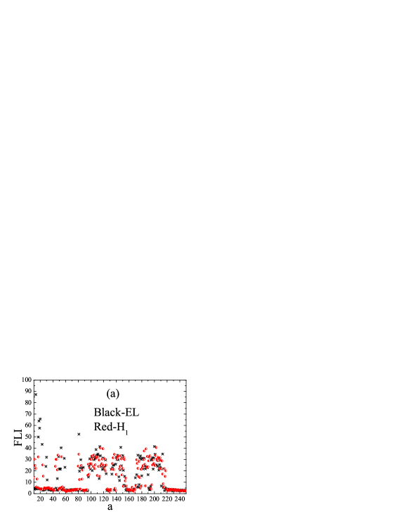
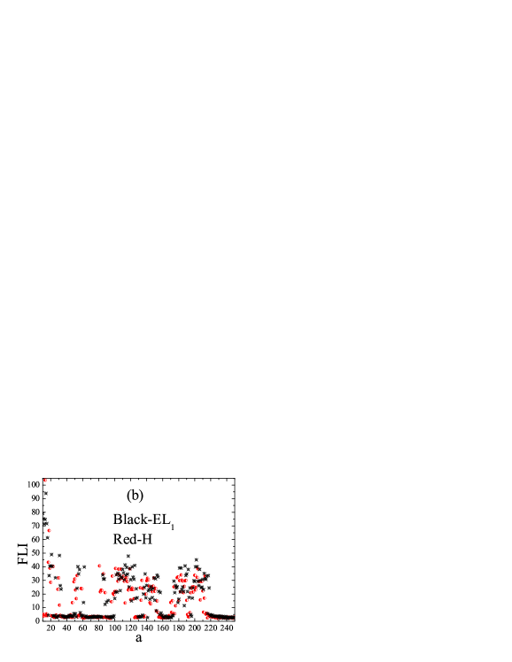
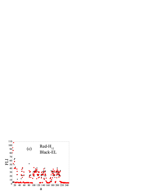
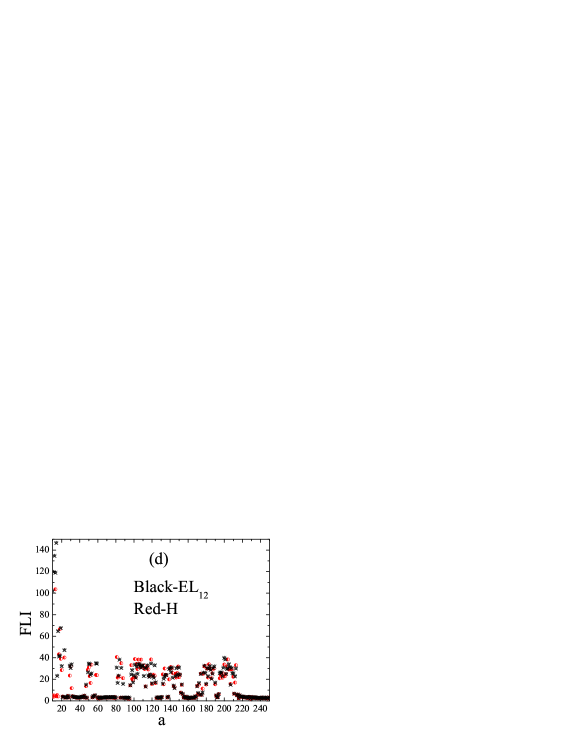
Figure 4: (color online) Dependence of FLIs on the separation $a$.

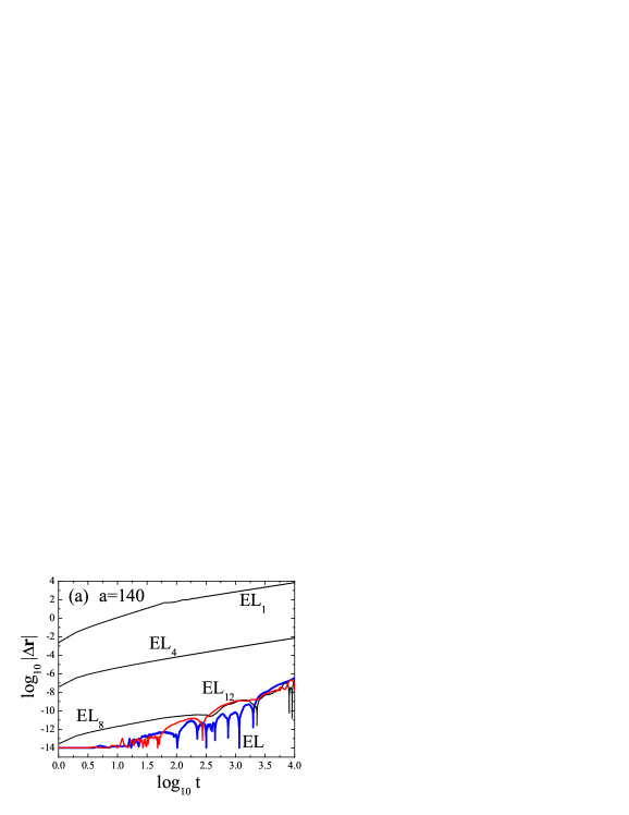
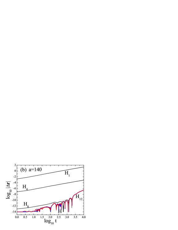
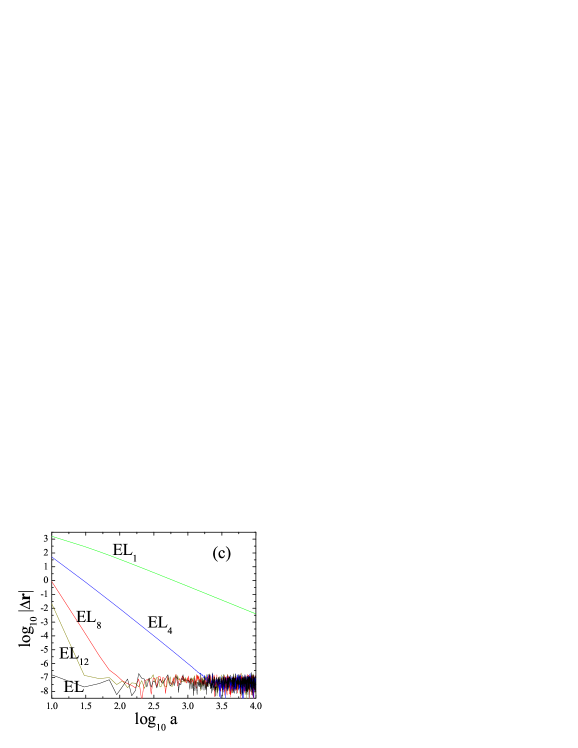
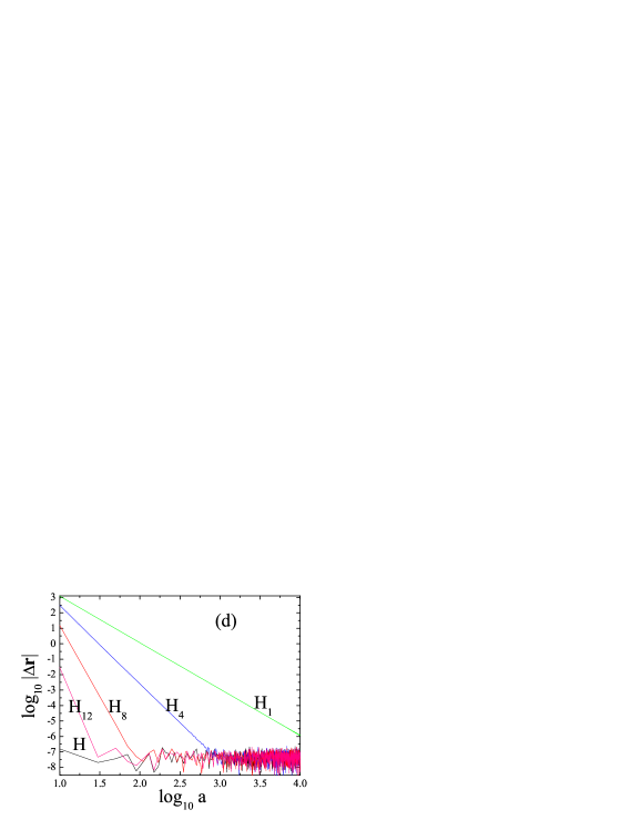
Figure 5: (color online) Deviation $|\Delta\mathbf{r}|$ between position solutions of the related PN Lagrangian and Hamiltonian formulations. Panels (a) and (c) are the deviations from $H$ to $EL$, $EL_{i}$ ($i=1,4,8,12$). Panels (b) and (d) deal with the deviations from $EL$ to $H$, $H_{i}$.