Spin-orbit torque driven chiral magnetization reversal in ultrathin nanostructures

Abstract

We show that the spin-orbit torque induced magnetization switching in nanomagnets presenting Dzyaloshinskii-Moriya (DMI) interaction is governed by a chiral domain nucleation at the edges. The nucleation is induced by the DMI and the applied in-plane magnetic field followed by domain wall propagation. Our micromagnetic simulations show that the DC switching current can be defined as the edge nucleation current, which decreases strongly with increasing amplitude of the DMI. This description allows us to build a simple analytical model to quantitatively predict the switching current. We find that domain nucleation occurs down to a lateral size of $15\;$nm, defined by the length-scale of the DMI, beyond which the reversal mechanism approaches a macrospin behavior. The switching is deterministic and bipolar

The recent discovery that a current can switch the magnetization of a nanomagnet in ultrathin heavy metal (HM)/Ferromagnetic (FM) multilayers has opened a new path to manipulate magnetization at the nanoscale Miron et al. (2011). The switching arises from structural inversion asymmetry and high spin-coupling, resulting in a spin current from the HM into the FM. This novel switching mechanism has led to innovative magnetic memory concept, namely the spin-orbit torque MRAM Miron et al. (2011); Liu et al. (2012a); Cubukcu et al. (2014), which combines large endurance, low power, and fast switching and thus appears as a possible non-volatile alternative for cache memory applications. Recently, Garello et al. Garello et al. (2014) demonstrated deterministic magnetization switching by spin-orbit torque (SOT) in ultrathin Pt/Co/AlO_x, as fast as $180\;$ps. These observations could not be explained within a simple macrospin approach, suggesting a magnetization reversal mechanism by domain nucleation and domain wall (DW) propagation. The failure of the macrospin approach for quantitative description is also underlined by the predicted switching current density, which is nearly one order of magnitude larger than experimental ones Liu et al. (2012b); Lee et al. (2013, 2014a). Besides its fundamental importance, this lack of a proper quantitative modeling is an important issue for the design of logic and memory devices based on SOT switching, which have so far considered a macrospin description Kim et al. (2015); Jabeur et al. (2014a, b); Wang et al. (2015). The final ingredient is the presence of antisymmetric exchange interaction, i.e. Dzyaloshinskii-Moriya interaction (DMI). This exchange tends to form states of non-collinear magnetization, promoting homochiral Néel DW  Chen et al. (2013); Thiaville et al. (2012); Tetienne et al. (2015). In the Néel configuration, a maximal SOT is applied on the DW  Thiaville et al. (2012); Emori et al. (2013); Boulle et al. (2013); Ryu et al. (2013). This explains the large current induced DW velocity observed experimentally Miron et al. (2011); Ryu et al. (2013). Moreover, the DMI can result in significant magnetization tilting at the edges of magnetic structures, resulting, e.g., in asymmetric field induced domain nucleation Rohart and Thiaville (2013); Pizzini et al. (2014). The influence of the DMI on the magnetization pattern during SOT switching was recently pointed out in micromagnetic simulation studies Perez et al. (2014); Finocchio et al. (2013); Martinez et al. (2015), whereas recent experimental work Lee et al. (2014b) explained the SOT switching mechanism by the expansion of a magnetic bubble.

Here, using micromagnetic simulations and analytic modeling, we show that the SOT-induced magnetization switching in the presence of DMI is governed by domain nucleation on one edge followed by propagation to the opposite edge. This reversal process allows to explain the ultra-fast deterministic switching observed experimentally. We systematically demonstrate that DMI leads to a large decrease of the switching current and of the switching time and thus strongly affects the reversal energy. On the basis of our micromagnetic simulations, we provide a simple analytical model which allows to quantitatively predict the SOT switching current in the presence of DMI. Finally, we address the evolution of the switching mechanism as the lateral dimension decreases, which is a key feature for the device scalability.

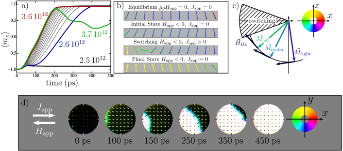
Figure 1: (color online) a) Time evolution of the average out-of-plane magnetization for different applied current densities (variations in steps of $10^{11}\;\mathrm{A/m}^{2}$). The minimum current to trigger switching, i.e.  the critical current, is highlighted in blue. The green curve indicates the threshold of turbulent behavior (see text). b) Sketch of the magnetization configuration at different stages of the switching process. c) Magnetization orientation in the center and at the left and right edges. The current induced damping-like torque (represented as effective field $\vec{H}_{\text{DL}}$) can only drive the left edge magnetization into instability, resulting in a nucleation at the left edge. d) Snap-shots of the magnetization configuration showing the reversal from down (black) to up (white) via domain wall nucleation and propagation under an externally applied field of $\mu_{0}H=0.1\;$T and a current density of $2.6\;10^{12}\;\mathrm{A/m}^{2}$.

The structures considered in this study are similar to the one used by Garello et al. Garello et al. (2014): a perpendicularly magnetized Co circular nanodot on top of a Pt stripe and capped with alumina. The DMI is included into the simulation using the expression of Ref. Thiaville et al. (2012). In addition to the standard micromagnetic energy density (which includes the exchange, the magnetocrystalline anisotropy, the Zeeman and the demagnetizing energy), the current injected in the Pt layer leads to two SOT terms in the the Landau-Lifshitz-Gilbert equation: the field-like $T_{\text{FL}}\propto\vec{m}\times\vec{e}_{y}$ and the damping-like $T_{\text{DL}}\propto\vec{m}\times(\vec{m}\times\vec{e}_{y})$, where $\vec{e}_{y}$ is the unit vector in $y$-direction (see spo for additional details). If not mentioned otherwise the external applied field is $\mu_{0}H_{\text{app}}=-0.1\;$T, and the material parameters are Garello et al. (2013): the saturation magnetization $M_{\mathrm{S}}=1090\;$kA/m, the exchange constant $A_{\text{ex}}=1.0\times 10^{-11}\;$A/m, the perpendicular magnetic anisotropy constant $K_{\text{u}}=1248\;\mathrm{kJ}/\mathrm{m}^{3}$, the DMI amplitude $D=2\;\mathrm{mJ}/\mathrm{m}^{2}$, the Gilbert damping parameter $\alpha=0.5$, the torques $T^{0}_{\text{FL}}=-0.05\;\text{pT}\text{m}^{2}/\text{A}$ and $T^{0}_{\text{DL}}=+0.1\;\text{pT}\text{m}^{2}/\text{A}$.

The 3D micromagnetic simulations are performed using the solver Micro3D Buda et al. (2002) with a mesh size smaller than $1.5\;$nm. The initial magnetization state of the dot is the remanent state after saturation by a negative magnetic field ($-O_{z}$) as shown for $0\;$ps in Fig. 1 d). In the presence of an applied magnetic field $\vec{H}_{\text{app}}$ in the $x$-direction, magnetization dynamics is induced by a current pulse with a rise (and fall) time of $50\;$ps and variable width and amplitude. Typical simulation results of a $100\;$nm dot are presented in Fig. 1 a). Depending on the current amplitude, three regimes are identified:

1) For $J_{\text{app}}\leq 2.50\;10^{12}\;\mathrm{A/m}^{2}$ no magnetization switching is observed. The SOT leads to a slight tilting of the magnetization toward the plane of the dot, but the magnetization relaxes toward its initial equilibrium state after the pulse.

2) At intermediate current values ($2.60\;10^{12}\;\mathrm{A/m}^{2}\leq J_{\text{app}}\leq 3.70\;10^{12}\;\mathrm{A/m}^{2}$) magnetization reversal occurs. The time evolution of the magnetization pattern in the dot, see Fig. 1 d) reveals that, in contrast to recent interpretations Lee et al. (2014b), the magnetization reversal occurs by domain nucleation shortly after the pulse injection ($100\;$ps), followed by fast DW propagation. The nucleation always occurs on the left edge of the dot. Once nucleated, the DW propagates fast through the dot and is expelled on the opposed edge. The switching time $t_{0}$, defined by $\langle m_{z}\rangle(t=t_{0})=0$, decreases as $J_{\text{app}}$ increases; the increase of the slope of $\langle m_{z}\rangle(t)$ indicates that this is related to a faster DW propagation. As expected the DW has a Néel configuration due to the large DMI. The simulation highlights that the DW nucleation occurs for all current values on the same edge in a deterministic way. Symmetrically, when reversing the sign of the current, the reversal from the up to the down state occurs on the opposite edge, i.e. the behavior is bipolar.

3) For higher currents ($J_{\text{app}}\geq 3.70\;10^{12}\;\mathrm{A/m}^{2}$) the motion of the DW becomes turbulent (oscillatory) and the coherence of the switching is destroyed.

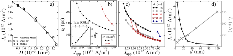
Figure 2: (color online) a) Critical current for destabilizing the system as a function of DMI strength. b) The relation between the critical current and the switching time $t_{0}$ for two different values of DMI.The inset show the data for $D=2\;\text{mJ/m}^{2}$, but in a transformed coordinate system $J_{\text{app}}$ verus $t_{0}^{-1}$. c) The switching time versus current for different dot diameters. d) Critical current and current density for different dot sizes. The calculation of the current assumes a 3 nm thick Pt line.

The magnetization reversal scheme can be explained in a simplified manner by considering the combined effect of DMI, external magnetic field, and SOT, but neglecting small variations of the demagnetizing field Meckler et al. (2012). The DMI is too small to introduce a spin spiral but results in a magnetization canting at the dot edges Rohart and Thiaville (2013); Pizzini et al. (2014); Martinez et al. (2015). The edge canting can be considered as an additional effective field with spacial variation: on one side this field adds to the in-plane applied field, while it counteracts on the other (see Fig. 1 b). This leads to an asymmetric tilting of the magnetization on both edges.

Upon current injection the damping-like torque emerges. Its effect can be interpreted as a rotating magnetic field of the form $\vec{H}_{\text{DL}}\propto J_{\text{app}}\vec{m}\times\vec{e}_{\mathrm{y}}$ (see Fig. 1 c)). This leads to a rotation of the magnetization towards the film plane on one side and away from the film plane on the other. Naturally, the current polarity is chosen such that the stronger tilted edge magnetization turns towards the film plane. Above a critical current an instability occurs, leading to domain nucleation and consecutive DW propagation. It is clear that the current $J_{\mathrm{c}}$, required to introduce the instability, reduces with increasing DMI. This behavior is seen in Fig.2 a), where $J_{\mathrm{c}}$ tends to zero when $D\approx 3.8\;\mathrm{mJ/m}^{2}$. Moreover, for $J_{\text{app}}>J_{\mathrm{c}}$ an increase of DMI decreases the switching time, as can be seen from Fig. 2 b). After expelling the DW on the opposite side, switching has occurred and the more tilted edge appears on the opposite side. As the SOT rotates this side away from the film plane and is not sufficient to rotate the less tilted side into instability, the state is, hence, stable. It can be easily checked that this reversal scheme is in agreement with the hysteretic bipolar switching observed experimentally when sweeping $J_{\text{app}}$ and $H_{\text{app}}$ Miron et al. (2011).

To understand these results better, we consider a simple analytical model, which describes the reversal process in the presence of both DMI and SOT. Using a Lagrangian approach and following Pizzini et al. Pizzini et al. (2014), the strategy is, eventually, similar to the Stoner-Wohlfarth approach in a single domain particle but using the energy functional

$$\frac{E(\theta)}{V}=-K_{\text{eff}}\cos^{2}\theta-M_{\text{S}}H_{\text{app}}\sin\theta-M_{\mathrm{S}}J_{\text{app}}T_{\text{DL}}\theta,$$ (1)

where the effect of the SOT is introduced by the last term spo . The equilibrium magnetization angle in the center, $\theta_{\mathrm{c}}$ is found by minimizing Eq. 16, while edge angle $\theta_{\mathrm{e}}$ is found by solving $[E(\theta_{\mathrm{e}})-E(\theta_{\mathrm{c}})]/V=0.25D^{2}A^{-1}$ spo . For small SOT and $\vec{H}_{\text{app}}$, two stable solutions for $\theta_{\mathrm{e}}$ exist, corresponding to both sample edges. Above a threshold SOT one solution disappears, indicating that the magnetization on one edge is unstable, i.e. domain nucleation occurs. Using numerical methods, the critical current for nucleation $J_{\mathrm{c}}$ can be calculated easily as a function of $D$ (see Fig. 2 a), black line). A good agreement is obtained with micromagnetic simulation for a dot diameter $d=100\;$nm (circles). For $D$ tending to zero, the nucleation current tends to the critical current predicted by the macrospin model $J_{\mathrm{c}}=4.1\times 10^{12}\;\text{A/m}^{2}$ Lee et al. (2013). The absence of full quantitative agreement with micromagnetic simulation can be attributed to variations of the demagnetizing tensor and variations of the magnetization along the $y$-direction due to the curvature of the dot. Better agreement is obtained when neglecting these effects in a quasi 1D simulation (square dots). Note that this nucleation current is actually the threshold current for quasi-DC current pulse.

In the following, we discuss the dynamics of the magnetization switching. In Fig. 2b) the switching time is shown as a function of $J_{\mathrm{app}}>J_{\mathrm{c}}$. With increasing $J_{\mathrm{app}}$ the switching time decreases rapidly as the DW velocity increases Boulle et al. (2013). If $D$ is reduced, the DW propagation is slower, resulting in a larger switching time. In the inset we show $J_{\text{app}}$ versus $1/t_{0}$ for $D=2\;\text{mJ/m}^{2}$: a linear scaling is observed, in qualitative agreement with experiment Garello et al. (2014).

Naturally, $t_{0}$ depends on the dot diameter. This is a key parameter for SOT applications. The evolution of switching time versus current density for varying dot sizes is shown in Fig. 2 c). When decreasing the diameter from $100\;$nm down to $50\;$nm, a shift to shorter switching times is observed while a slightly higher onset current is found. Similar behavior is found when decreasing the size down to $30\;$nm and further down to $25\;$nm. It is, however, important to note that the latter two graphs become identical for larger $J_{\text{app}}$. Reducing the size down to $15\;$nm, results in a dramatic increase of the threshold current density. Moreover, deterministic switching is observed in a narrow current density region only. Overall one has indications for three different size-dependent switching regimes. In the first regime the switching is covered by nucleation and propagation of a DW and the decrease of $t_{0}$ is mainly caused by a reduced distance for the DW to travel. In the second regime the switching remains governed by DW propagation. The diameter, however, becomes comparable to approximately twice the value of $\xi=2A/D\approx 10$ nm, the characteristic length scale on which canting of the edge magnetization is observed. In this situation the edge angle due to DMI differs from the ideal infinite case and opposite edges are not completely independent anymore (see Ref. spo ). While this does not cause coherent rotation yet, it affects the DW motion. The coherent regime is reached at diameters in the range of the DW width $\Delta=\pi\sqrt{A/K_{\text{eff}}}\approx 14\;$nm. This explains the significant change in switching behavior for the $15\;$nm dot. Note that the switching current at this size is close to the one predicted by macrospin simulation ($4.1\times 10^{12}\;\text{A/m}^{2}$). It is worth mentioning that while the current density strongly increases with decreasing dot diameter, the current in the $3\;$nm thick Pt stripe decreases almost linearly, as can be seen from Fig. 2 d). Therefore, the device exhibits favorable scaling behavior and assuming a $1\;\mathrm{k}\Omega$ resistance for the addressing transistor of a $30\;$nm dot, switching in about $300\;$ps, needs only $20\;$fJ for one switching event, which is significantly smaller than the energy for perpendicular spin-transfer torque devices Liu et al. (2014).

Naturally, the threshold current and switching time depend on several intrinsic as well as extrinsic parameters. We have studied in detail the influence of the applied field, the damping constant, the strength of the field like torque, and temperature. The results are shown in Fig. 3. Variations in these parameters lead to quantitative changes of the nucleation current as well as the switching time. In all cases this is mainly attributed to changes in DW velocity; lower damping increases the wall velocity and so does an in-plane field, as it promotes and stabilizes a Néel type wall. A negative field like torque also stabilizes the DW, while a positive one destabilizes it, therefore increasing the switching time. The edge nucleation/DW propagation mechanism, however, is not affected.

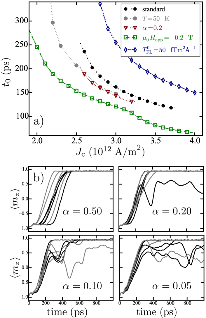
Figure 3: (color online) a) Switching time as a function of applied current density, varying intrinsic and extrinsic parameters. For the temperature case, the average $t_{0}$ is plotted. The single event switching time is defined as before, while the average $t_{0}$ is defined as the time where the probability of stochastical switching reaches $90\%$. b) Several switching graphs $\langle m_{z}\rangle(t)$ for varying damping at $T=50\;$K and $J_{\text{app}}=2.6\;10^{12}\;\mathrm{A/m}^{2}$. For fixed $\alpha$ variations are only due to temperature fluctuations.

Most importantly Fig. 3 a) shows that the mechanism of switching by nucleation and propagation is very robust against fluctuations due to temperature (See Ref. spo for more details). The temperature fluctuations strongly decrease the threshold current (Fig. 3 b). Temperature effectively lowers the nucleation barrier, such that nucleation times get shorter and, consequently, the whole switching becomes faster. It has to be pointed out that the nucleation still takes place at the same position on the dot edge and the overall process remains bipolar with respect to field and current reversal. This temperature robustness, however, strongly relies on the large damping, as can be seen from Fig. 3 b). With decreasing $\alpha$ an increasing tendency of oscillations is observed, such that deterministic switching cannot be guaranteed Lee et al. (2013).

To conclude, we have studied the current induced magnetization switching of a nanomagnet by spin-orbit torques in the presence of Dzyaloshinskii-Moryia interaction (DMI). The critical switching current strongly decreases with increasing amplitude of DMI and we provide a simple analytical model for this dependency. This switching mechanism via chiral domain nucleation explains the deterministic switching observed experimentally in ultra thin Pt/Co/AlO_x even for sub-ns pulses. The switching is mainly introduced by the damping like torque, but the field like torque cannot be neglected as it strongly influences the switching time. Our systematic studies show a change in the reversal mechanism below diameters of $30\;$nm, while the switching remains deterministic and bipolar. However, at $0\;$K the operational window for current densities decreases with decreasing dot diameter. The influence of temperature on this technological important limit will be investigated in the future. Most importantly, current scalability is maintained. Confirming the potential of SOT-MRAM for scalable fast non-volatile memory application, our results will help in the design of devices based on this technology.

This work was funded by the spOt project(318144) of the EC under the Seventh Framework Programme.

Appendix A Appendix

A.1 General description of sample and technics

The properties of cobalt films sandwiched between platinum and a insulating oxide such as AlO are studied. Due to the different substrate and capping materials the inversion symmetry is broken along the vertical axis ($\mathcal{O}z$). The magnetization is oriented out-of-plane with a strong magnetocrystalline perpendicular anisotropy. In addition to the standard micromagnetic energy density, which includes the exchange, the magnetocrystalline anisotropy, the Zeeman and the demagnetizing energy, the Dzyaloshinskii-Moriya contribution is included according to the following relation:

$$E_{\text{DM}}=D\left[m_{z}\frac{\partial m_{x}}{\partial x}-m_{x}\frac{\partial m_{z}}{\partial x}+m_{z}\frac{\partial m_{y}}{\partial y}-m_{y}\frac{\partial m_{z}}{\partial y}\right]$$ (2)

This expression corresponds to a sample isotropic in the $x$-$y$-plane, where the Dzyaloshinskii vector for any in-plane direction $\vec{e}_{u}$ is $D(\vec{e}_{z}\times\vec{e}_{u})$ with $D$ a uniform constant, originating from the symmetry breaking at the $z$-surface Thiaville et al. (2012), and $\vec{e}_{u}$ being the unit vector in direction of an arbitrary $\vec{u}$.

Micromagnetic simulations are based on the time integration of Landau-Lifshitz-Gilbert equation including the field-like $T_{\text{FL}}$ and damping-like $T_{\text{DL}}$ spin-orbit torques:

$$\frac{\mathrm{d}\vec{m}}{\mathrm{d}t} = -\gamma_{0}\left[\vec{m}\times(\vec{H}_{\text{eff}}+\vec{H}_{\text{DM}})\right]+\alpha\left(\vec{m}\times\frac{\mathrm{d}\vec{m}}{\mathrm{d}t}\right)+$$ (3)

$$+\vec{T}_{\text{FL}}+\vec{T}_{\text{DL}}$$

Here $\vec{m}$ is the unitary vector of the magnetization, $\alpha$ is the Gilbert damping parameter, $\gamma_{0}$ is the product of the vacuum permeability $\mu_{0}$ and the free electron gyromagnetic ratio $\gamma$. For the spin-orbit torques only the first order terms are considered, namely $\vec{T}_{\text{FL}}=\gamma T^{0}_{\text{FL}}J_{\text{app}}(\vec{m}\times\vec{e}_{y})$ and $\vec{T}_{\text{DL}}=\gamma T^{0}_{\text{DL}}J_{\text{app}}\vec{m}\times(\vec{m}\times\vec{e}_{y})$, where $T^{0}_{\text{FL}}=-0.05\;\text{pT}\text{m}^{2}/\text{A}$ and $T^{0}_{\text{DL}}=+0.1\;\text{pT}\text{m}^{2}/\text{A}$ are scalar constants. Higher order terms can be found in Garello et al. (2013).

The appearance of $\vec{e}_{y}$ in the definition of the torques is a simplification due to currents in $\vec{e}_{x}$. In the general case this must be replaced by $\vec{e}_{y}\rightarrow\vec{e}_{u}=\vec{e}_{z}\times\vec{e}_{j}$, where $\vec{e}_{j}$ is the unit vector in the direction of the conventional current, i.e. opposite to the electron flow.

Appendix B Lagrange formalism for damping like spin-torque

The LLG equation in spherical coordinates ($\theta,\phi$) can be derived from a Lagrangian by defining a pseudo kinetic energy Wegrowe and Ciornei (2012) of the form

$$E_{\text{kin}}=-\frac{M_{\text{S}}}{\gamma}\dot{\phi}\cos\theta,$$ (4)

where the dot-notation refers to the total time derivative. With $U$ as potential energy, the equation of motion is derived from the action

$$\mathcal{L}=E_{\text{kin}}-U,$$ (5)

in the typical form of

$$\frac{\delta\mathcal{L}}{\delta q}-\frac{\mathrm{d}}{\mathrm{d}t}\frac{\delta\mathcal{L}}{\delta\dot{q}}=\frac{\delta F}{\delta\dot{q}},$$ (6)

where $\delta$ refers to the functional derivative and $q\in\{\theta,\phi\}$. Here we add a dissipative term $F$ of the form

$$F=\frac{\alpha M_{\text{S}}}{2\gamma}\left(\frac{\mathrm{d}}{\mathrm{d}t}\vec{m}+\frac{\chi}{\alpha}\vec{m}\times\vec{e}_{y}\right)^{2}$$ (7)

and $\chi=\gamma T^{0}_{\text{DL}}J_{\text{app}}$. The square of the first term in parenthesis of Eq. 7 results in the standard damping of the LLG equation. The square of the second term vanishes when evaluating Eq. 6, while the mixed term results in the damping-like torque. Using a quasi 1D case with potential energy of the form

$$U=A\theta_{x}^{2}-D\theta_{x}-K_{\text{eff}}\cos^{2}\theta-\mu_{0}M_{\text{S}}H_{\text{app}}\sin\theta.$$ (8)

(here the index $x$ indicates the partial derivative with respect to $x$) and a field applied in $x$-direction one derives the equations of motion as.

$$\frac{M_{\text{S}}}{\gamma}\dot{\phi}\sin\theta-K_{\text{eff}}\sin 2\theta+2A\theta_{xx}+$$

$$+\mu_{0}M_{\text{S}}H_{\text{app}}\cos\theta-\frac{\alpha M_{\text{S}}}{\gamma}\dot{\theta}+\frac{M_{\text{S}}}{\gamma}\chi\cos\phi = 0$$ (9)

$$\frac{M_{\text{S}}}{\gamma}\dot{\theta}\sin\theta+\frac{\alpha M_{\text{S}}}{\gamma}\dot{\phi}\sin^{2}\theta+$$

$$+\frac{M_{\text{S}}}{\gamma}\chi\sin\phi\sin\theta\cos\theta = 0$$ (10)

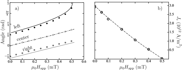
Figure 4: a) Angle of the magnetization with respect to the $z$-direction as a function of an applied magnetic field in $x$-direction and and zero current. Due to DMI the magnetization at the edges of the infinite long stripe differ from the center. At approximately $0.5\;$T the first edge is fully in-plane. Note, without current and due to symmetry the maximum edge angle is always $\pi/2$. b) Analytically calculated critical current $J_{\mathrm{c}}$, required to destabilize the system, plotted against an in-plane applied magnetic field. In both cases the analytical model (continuous lines) is well reproduced by a micromagnetic simulation (dots) for a stripe of width $200\;$nm ($128$ cells) and a constant effective anisotropy. The other parameters are given in the text.

Note that the DMI drops out when applying the functional derivative. In the quasi static case of $\dot{\theta}=\dot{\phi}=0$ this simplifies to

$$-K_{\text{eff}}\sin 2\theta+2A\theta_{xx}+\mu_{0}M_{\text{S}}H_{\text{app}}\cos\theta+$$

$$+\frac{M_{\text{S}}}{\gamma}\chi\cos\phi = 0$$ (11)

$$\frac{M_{\text{S}}}{\gamma}\chi\sin\phi\sin\theta\cos\theta = 0$$ (12)

The second equations is already consistently fulfilled by setting $\phi=n\pi$, $n\in\mathbb{Z}_{0}$, i.e. the quasi 1D case in the $x$-$z$-plane. It remains to solve

$$-K_{\text{eff}}\sin 2\theta+2A\theta_{xx}+\mu_{0}M_{\text{S}}H_{\text{app}}\cos\theta\pm\frac{M_{\text{S}}}{\gamma}\chi=0$$ (13)

Multiplying by $\theta_{x}$ allows to integrate resulting in

$$A\theta^{2}_{x}=-K_{\text{eff}}\cos^{2}\theta-\mu_{0}M_{\text{S}}H_{\text{app}}\sin\theta\mp\frac{M_{\text{S}}}{\gamma}\chi\theta+C,$$ (14)

where C is the integration constant. This result is identical to Ref. Pizzini et al. (2014) except for the linear term due to the damping like torque, i.e. $g(J_{\text{app}})\theta$ with $g(J_{\text{app}})=M_{\text{S}}J_{\text{app}}T^{0}_{\text{DL}}$.

Appendix C Analytical model for the critical current at 0 K

A simplified analytical model has been developed, which already exhibits the important mechanisms of the behavior observed in experiment. An important ingredient for deterministic switching in the analytical model is the presence of DMI. The DMI in the presented material system is below the critical value, such that no spin spiral is formed. Due to the boundary condition

$$\frac{D}{2A}\left(\vec{e}_{z}\times\vec{n}\right)\times\vec{m}=\nabla_{\vec{n}}\vec{m}$$ (15)

and the finite size of the sample, however, the magnetization is not homogeneous and canting is observed at the edges. Here $\vec{n}$ is the surface normal and $\nabla_{\vec{n}}$ the normal derivative. It has been shown recently that the canting angle at the edge as well as in the center of the sample can be evaluated using simple energy arguments Pizzini et al. (2014), provided that the demagnetizing energy can be approximated by an effective anisotropy. This is not always the case Meckler et al. (2012), but for the given parameters it is justified as can be seen from Rohart and Thiaville (2013). The derived angles from this simple analytical calculation and a micromagnetic simulation that accounts for the demagnetization energy by an effective anisotropy, are in very good agreement, as can be seen from Fig. 4 a). As the micromagnetic angle is taken from the cell magnetization, a small deviation to the theoretical edge value is observed. With decreasing mesh size this deviation decreases. The original publication Pizzini et al. (2014) calculates a critical magnetic field in $z$-direction resulting in the nucleation of a domain. In the present case the according term is substituted by a current dependent term (see paragraph B), taking account for the dominant damping like torque. At first glance this is problematic, as the model considers a static case approaching an instability. Moreover, it is 2D in the sense that it assumes $m_{y}=0$, while a damping like torque initially acts along the $y$-direction. For large damping, however, changes of the magnetization become quasi static and mainly take place in the $x$-$z$-plane.

To provide the full solution for $\theta=\theta(x)$ one needs to integrate Eq. 14. In the center of the sample, i.e. far away from the edges, one can assume $\theta_{x}=0$, such that the DMI drops out again. The total energy density, hence, has the form

$$\frac{E(\theta)}{V}=-K_{\text{eff}}\cos^{2}\theta-M_{\mathrm{S}}H_{\text{app}}\sin\theta-g(J_{\text{app}})\theta$$ (16)

and the equilibrium angle is found by minimizing Eq. 16. A second position where one can find a solution is the edge. Here additional information is given by the boundary condition Eq. 15. Inserting the boundary conditions into Eq. 14 results in Eq. 16 plus an additional offset $\Delta E$ of

$$\frac{\Delta E}{V}=\frac{D^{2}}{4A}$$ (17)

As a result the solution of the edge angle is given by a value $\theta$ that has a $\Delta E$ higher energy than the minimum energy in the DMI free energy landscape of Eq. 16. Hence, a stable solution for the edge angle can only be found if the energy landscape provides a value of $\Delta E$ above the local minimum, i.e. above the solution of the center angle. For a small current the edge solution corresponds to a point near the next local maximum. With increasing current this local maximum decreases and at the critical current $J_{\mathrm{c}}$, it is separated from the minimum by exactly $\Delta E$. Eventually, the solution for the magnetization angle at the sample edge vanishes for larger currents, i.e. the current drives the system into instability. The results of the analytical model for current driven instabilities are plotted as continuous line in Figure 4 b). The analytical values are compared to a simple simulation neglecting variations of the demagnetizing field and assuming only an effective anisotropy. The agreement of analytical results and simulation are in astonishing agreement. The applicability of the model is, however, limited as it neglects temperature. It is shown below that temperature has a significant effect on the critical current.

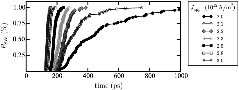
Figure 5: Accumulated switching probability as function of time for different current densities at $T=50\;$K.

Appendix D Thermal fluctuations and switching probabilities

The temperature was included in the form of a Gaussian distributed thermal field $\vec{H}_{\text{th}}$, which is added to the effective field $\vec{H}_{\text{eff}}$. The thermal fluctuations have the following properties Brown Jr. (1963):

$$\langle H_{\text{th},i}(t)\rangle=0$$ (18)

and

$$\langle H_{\text{th},i}(t)H_{\text{th},j}(t^{\prime})\rangle=\frac{2\alpha k_{\mathrm{B}}T}{\mu_{0}V_{\text{cell}}}\delta_{ij}\delta\left(\gamma_{0}M_{\text{S}}(t-t^{\prime})\right)$$ (19)

where $k_{\mathrm{B}}$ is the Boltzmann constant and $V_{\text{cell}}$ the volume of the discretization cell. As temperature results in stochastic behavior of switching one has to consider switching probabilities. This is done by evaluating 100 independent switching events for each parameter set. For each event the the switching time $t_{0}$, i.e. the time when $\langle m_{z}\rangle$ crosses zero is determined. From this the integrated probability is calculated. A typical result is shown in Fig. 5. The overall switching time in the presence of thermal fluctuations is then defined as the time where the integrated probability reaches 90%. Naturally, the switching time decreases with increasing current density. One has to keep in mind, however, that this data representation does not give information about oscillatory behavior for larger times beyond the (first) zero crossing of $\langle m_{z}\rangle$. This graph, hence, can pretend fast switching where actually oscillatory behavior is present.

Appendix E Size dependence

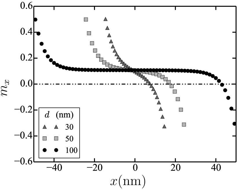
Figure 6: Cross section showing $m_{x}$ for different dot diameters and a $100\;$mT applied field $x$-direction. Within approximately $20\;$nm the canting at the edge decays towards a homogeneous magnetization at the dot center.

In addition to the exchange length, the system at hand exhibits a second important length scale. This length is given by the interplay of DMI and exchange interaction, i.e., to what extend the non-collinear magnetism from the edge penetrates the sample. The according length is given by $\xi=2A/D\approx 10\;$nm. It can be seen from Fig. 6 that this length scale becomes relevant for dot diameters below approximately $40\;$nm. For smaller diameters a strictly monotonic change of $m_{z}$ is observed while larger diameters present a center plateau.

References

- Miron et al. (2011) I. Miron, K. Garello, G. Gaudin, P.-J. Zermatten, M. V. Costache, S. Auffret, S. Bandiera, B. Rodmacq, A. Schuhl, and P. Gambardella, Nature 476, 189 (2011).
- Liu et al. (2012a) L. Liu, C.-F. Pai, Y. Li, H. W. Tseng, D. C. Ralph, and R. A. Buhrman, Science 336, 555 (2012a).
- Cubukcu et al. (2014) M. Cubukcu, O. Boulle, M. Drouard, K. Garello, C. Avci, I. Miron, J. Langer, B. Ocker, P. Gambardella, and G. Gaudin, Appl. Phys. Lett. 104, 042406 (2014).
- Garello et al. (2014) K. Garello, C. Avci, I. Miron, M. Baumgartner, A. Ghosh, S. Auffret, O. Boulle, G. Gaudin, and P. Gambardella, Appl. Phys. Lett. 105, 212402 (2014).
- Liu et al. (2012b) L. Liu, O. J. Lee, T. J. Gudmundsen, D. C. Ralph, and R. A. Buhrman, Phys. Rev. Lett. 109, 096602 (2012b).
- Lee et al. (2013) K.-S. Lee, S.-W. Lee, B.-C. Min, and K.-J. Lee, Appl. Phys. Lett. 102, 112410 (2013).
- Lee et al. (2014a) K.-S. Lee, S.-W. Lee, B.-C. Min, and K.-J. Lee, Appl. Phys. Lett. 104, 072413 (2014a).
- Kim et al. (2015) Y. Kim, X. Fong, K.-W. Kwon, M.-C. Chen, and K. Roy, IEEE T. Electron Dev. 62, 561 (2015).
- Jabeur et al. (2014a) K. Jabeur, G. Di Pendina, and G. Prenat, Electron. Lett. 50, 585 (2014a).
- Jabeur et al. (2014b) K. Jabeur, G. Di Pendina, G. Prenat, L. D. Buda-Prejbeanu, and B. Dieny, IEEE T. Magn. 50, 1 (2014b).
- Wang et al. (2015) Z. Wang, W. Zhao, E. Deng, J.-O. Klein, and C. Chappert, J. Phys. D: Appl. Phys. 48, 065001 (2015).
- Chen et al. (2013) G. Chen, J. Zhu, A. Quesada, J. Li, A. T. N’Diaye, Y. Huo, T. P. Ma, Y. Chen, H. Y. Kwon, C. Won, Z. Q. Qiu, A. K. Schmid, and Y. Z. Wu, Phys. Rev. Lett. 110, 177204 (2013).
- Thiaville et al. (2012) A. Thiaville, S. Rohart, E. Jué, V. Cros, and A. Fert, Eur. Phys. Lett. 100, 57002 (2012).
- Tetienne et al. (2015) J.-P. Tetienne, T. Hingant, L. J. Martínez, S. Rohart, A. Thiaville, L. H. Diez, K. Garcia, J.-P. Adam, J.-V. Kim, J.-F. Roch, I. M. Miron, G. Gaudin, L. Vila, B. Ocker, D. Ravelosona, and V. Jacques, Nat. Comm. 6, 6733 (2015).
- Emori et al. (2013) S. Emori, U. Bauer, S.-M. Ahn, E. Martinez, and G. S. D. Beach, Nat. Mater. 12, 611 (2013).
- Boulle et al. (2013) O. Boulle, S. Rohart, L. D. Buda-Prejbeanu, E. Jué, I. Miron, S. Pizzini, J. Vogel, G. Gaudin, and A. Thiaville, Phys. Rev. Lett. 111, 217203 (2013).
- Ryu et al. (2013) K.-S. Ryu, L. Thomas, S.-H. Yang, and S. Parkin, Nat. Nano 8, 527 (2013).
- Rohart and Thiaville (2013) S. Rohart and A. Thiaville, Phys. Rev. B 88, 184422 (2013).
- Pizzini et al. (2014) S. Pizzini, J. Vogel, S. Rohart, L. D. Buda-Prejbeanu, E. Jué, O. Boulle, I. Miron, C. Safeer, S. Auffret, G. Gaudin, and A. Thiaville, Phys. Rev. Lett. 113, 047203 (2014).
- Perez et al. (2014) N. Perez, E. Martinez, L. Torres, S.-H. Woo, S. Emori, and G. Beach, Appl. Phys. Lett. 104, 092403 (2014).
- Finocchio et al. (2013) G. Finocchio, M. Carpentieri, E. Martinez, and B. Azzerboni, Appl. Phys. Lett. 102, 212410 (2013).
- Martinez et al. (2015) E. Martinez, L. Torres, N. Perez, M. A. Hernandez, V. Raposo, and S. Moretti, Sci. Rep. 5, 10156 (2015).
- Lee et al. (2014b) O.-J. Lee, L.-Q. Liu, C.-F. Pai, Y. Li, H.-W. Tseng, P. G. Gowtham, J. P. Park, D. C. Ralph, and R. A. Buhrman, Phys. Rev. B 89, 024418 (2014b).
- (24) “see supplementary material,” .
- Garello et al. (2013) K. Garello, I. Miron, C. Avci, F. Freimuth, Y. Mokrousov, S. Blügel, S. Auffret, O. Boulle, G. Gaudin, and P. Gambardella, Nat. Nanotec. 8, 587 (2013).
- Buda et al. (2002) L. D. Buda, I. Prejbeanu, U. Ebels, and K. Ounadjela, Comput. Mater. Sci. 24, 181 (2002).
- Meckler et al. (2012) S. Meckler, O. Pietzsch, N. Mikuszeit, and R. Wiesendanger, Phys. Rev. B 85, 024420 (2012).
- Liu et al. (2014) H. Liu, D. Bedau, J. Z. Sun, S. Mangin, E. E. Fullerton, J. A. Katine, and A. D. Kent, J. Magn. Mag. Mater. 358–359, 233 (2014).
- Wegrowe and Ciornei (2012) J.-E. Wegrowe and M.-C. Ciornei, Am. J. Phys. 80, 607 (2012).
- Brown Jr. (1963) W. F. Brown Jr., Phys. Rev. 130, 1677 (1963).