Magnetic Behavior of Volborthite Cu₃V₂O₇(OH)${}_{2}\cdot$2H₂O
Determined by Coupled Trimers Rather than Frustrated Chains

Abstract

Motivated by recent experiments on volborthite single crystals showing a wide $\frac{1}{3}$-magnetization plateau, we perform microscopic modeling by means of density functional theory (DFT) with the single-crystal structural data as a starting point. Using DFT+$U$, we find four leading magnetic exchanges: antiferromagnetic $J$ and $J_{2}$, as well as ferromagnetic $J^{\prime}$ and $J_{1}$. Simulations of the derived spin Hamiltonian show good agreement with the experimental low-field magnetic susceptibility and high-field magnetization data. The $\frac{1}{3}$-plateau phase pertains to polarized magnetic trimers formed by strong $J$ bonds. An effective $J\rightarrow\infty$ model shows a tendency towards condensation of magnon bound states preceding the plateau phase.

The perplexing connection between quantum magnetism and topological states of matter renewed interest in frustrated spin systems Balents (2010). A prime example is the $S$ = $\frac{1}{2}$ antiferromagnetic kagome Heisenberg model (KHM), whose ground state (GS) can be a gapped topological spin liquid, as suggested by large-scale density-matrix renormalization group (DMRG) simulations Yan et al. (2011); Depenbrock et al. (2012). Although DMRG results were recently corroborated by nuclear magnetic resonance (NMR) measurements on herbertsmithite Fu et al. (2015), alternative methods vouch for a gapless spin liquid Iqbal et al. (2011, 2014) and the discussion is still not settled.

One of the remarkable properties of the KHM is the presence of field-induced gapped phases that manifest themselves as magnetization plateaus Nishimoto et al. (2013); Capponi et al. (2013); Schulenburg et al. (2002). A key ingredient thereof are closed hexagonal loops of the kagome lattice that underlie the formation of valence-bond solid states Capponi et al. (2013). By far widest is the $\frac{1}{3}$-magnetization plateau, whose structure is well described by singlets residing on closed hexagons, and polarized spins (Fig. 1, left) Nishimoto et al. (2013); Capponi et al. (2013); Schulenburg et al. (2002); Cabra et al. (2005).

Despite the considerable progress in understanding both quantum and topological aspects of the KHM, most theoretical findings still await their experimental verification. The reason is the scarceness of material realizations: only a handful of candidate KHM materials is known to date. A prominent example is herbertsmithite, where $S$ = $\frac{1}{2}$ spins localized on Cu²⁺ form a regular kagome lattice Helton et al. (2007). Other candidate materials feature exchange couplings beyond KHM as kapellasite Janson et al. (2008); Colman et al. (2008); Fåk et al. (2012); Jeschke et al. (2013); Iqbal et al. (2015); Bieri et al. (2015), haydeeite Janson et al. (2008); Colman et al. (2010); Boldrin et al. (2015); Iqbal et al. (2015); Bieri et al. (2015), francisite Rousochatzakis et al. (2015), or barlowite Han et al. (2014); Jeschke et al. (2015).

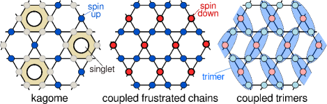
Figure 1: (Color online) The structure of the $\frac{1}{3}$-magnetization plateau in the kagome model (KHM), coupled frustrated chains (CFC) model from Ref. Janson et al. (2010), and the $J$-$J^{\prime}$-$J_{1}$-$J_{2}$ model.

The natural mineral volborthite Cu₃V₂O₇(OH)${}_{2}\cdot$2H₂O was considered a promising KHM material Hiroi et al. (2001); Bert et al. (2005), until it was noticed that the local environment of two crystallographically distinct Cu sites hints at different magnetically active orbitals Okamoto et al. (2009). Density functional theory (DFT) calculations show that this has dramatic implications for the spin physics, giving rise to coupled frustrated chains (CFC) with ferromagnetic (FM) nearest-neighbor and antiferromagnetic (AF) second-neighbor exchanges, and interstitial spins that are AF coupled to the two neighboring chains Janson et al. (2010). However, detailed structural studies reveal that below $\sim$300 K all Cu atoms have the $d_{x^{2}-y^{2}}$ as the magnetically active orbital Yoshida et al. (2012), questioning the applicability of the CFC model for volborthite. Furthermore, the CFC model features the $\frac{1}{3}$-magnetization plateau with a semiclassical “up-up-down” structure (Fig. 1, middle), which was never observed in powder samples Yoshida et al. (2009); Okamoto et al. (2011). Recent magnetization measurements on single crystals overturned the experimental situation: a broad $\frac{1}{3}$-magnetization plateau sets in at $H_{\text{c1}}\!\simeq$ 26 T and continues up to at least 74 T Ishikawa et al. (2015).

Puzzled by the remarkable difference between the single-crystal and powder data, we adopt the structural model from Ref. Ishikawa et al. (2015) and perform DFT and DFT+$U$ calculations. We find a microscopic model which is even more involved than CFC: besides sizable $J_{1}$ and $J_{2}$ forming frustrated spin chains, the coupling between the chain and the interstitial Cu atoms is now facilitated by two inequivalent exchanges, a sizable AF $J$ and a much weaker FM $J^{\prime}$. Due to the dominance of $J$, the magnetic planes break up into magnetic trimers (Fig. 2). By using exact diagonalization (ED) of the spin Hamiltonian, we demonstrate that this model agrees with the experimental magnetization data and explains the nature of the plateau phase (Fig. 1, right). Further insight into the low-field and low-temperature properties of volborthite is provided by analysing effective models of pseudospin-$\frac{1}{2}$ moments $T$ living on trimers. Thus, a model based on effective exchanges ${\cal J}_{1}$, ${\cal J}_{2}$ and ${\cal J}_{2}^{\prime}$ supports the presence of a bond nematic phase due to condensation of two-magnon bound states. Finally, we conjecture that powder samples of volborthite suffer from disorder effects pertaining to the stretching distortion of Cu octahedra.

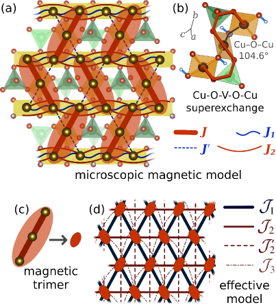
Figure 2: (Color online) (a) Microscopic magnetic model of volborthite featuring four relevant exchange couplings: antiferromagnetic $J$ (thick bars) and $J_{2}$ (solid curved lines), as well as ferromagnetic $J^{\prime}$ (dashed lines) and $J_{1}$ (wiggly lines). Magnetic trimers formed by $J$ exchanges are highlighted (shaded ovals). Magnetic Cu atoms are shown as large spheres within CuO₄ squares, nonmagnetic V atoms are middle-sized spheres within VO₄ tetrahedra. (b) The Cu-O-V-O-Cu superexchange paths in the magnetic trimer. (c) Magnetic trimers form a basis for (d) the effective model with ferromagnetic $\mathcal{J}_{1}$, as well as antiferromagnetic $\mathcal{J}_{2}$, $\mathcal{J}_{2}^{\prime}$, and $\mathcal{J}_{3}$.

We start our analysis with a careful consideration of the crystal structure. Volborthite features a layered structure, with kagome-like planes that are well separated by water molecules and non-magnetic V₂O₇ groups. Magnetic Cu²⁺ atoms within the planes occupy two different sites: Cu(2) with four short Cu–O bonds forms edge-sharing chains, and interstitial Cu(1) located in between the chains. Different structural models in the literature suggest either squeezed Basso et al. (1988); *volb:lafontaine90 or stretched Kashaev et al. (2008); *volb:ishikawa12 Cu(1)O₆ octahedra. The DFT study of Ref. Janson et al. (2010) employed a structure with a squeezed Cu(1) octahedron. Although such configuration can be realized at high temperatures Yoshida et al. (2012), Cu(1)O₆ octahedra are actually stretched in the temperature range relevant to magnetism Yoshida et al. (2012); Ishikawa et al. (2015). The respective structural model was never studied with DFT, hence we fill this gap with the present study.

For DFT calculations sup , we use the generalized gradient approximation (GGA) Perdew et al. (1996) as implemented in the full-potential code fplo9.07-41 Koepernik and Eschrig (1999). We start with a critical examination of all structural models proposed so far, by optimizing the H coordinates and comparing the total energies. In this way, we find that the single crystal structure of Ref. Ishikawa et al. (2015) has the lowest total energy sup . All further calculations are done for this structural data set.

To evaluate the magnetic couplings, we project the relevant GGA bands onto Cu-centered Wannier functions sup . The leading transfer integrals $t$ ($>$50 meV) of the resulting one-orbital ($d_{x^{2}-y^{2}}$) model are provided in Table 1. Their squared values are proportional to the AF superexchange, which is usually the leading contribution to the magnetism. However, such one-orbital model fully neglects FM contributions that are particularly strong for short-range couplings ($d_{\text{Cu..Cu}}$ $\lesssim$ 3 Å). Hence, to evaluate the exchange integrals that comprise AF and FM contributions, we perform DFT+$U$ calculations for magnetic supercells and map the total energies onto a Heisenberg model. These results are summarized in Table 1.

Table 1: Direct Cu..Cu distances $d_{\text{Cu..Cu}}$ (in Å), transfer integrals $t$ (in meV) and exchange integrals $J$ (in K). GGA+$U$ results are provided for three different values of the on-site Coulomb repulsion $U_{d}$. The two numbers in each entry pertain to the two structurally inequivalent layers; this minor layer dependence is ignored in the subsequent analysis.

	$d_{\text{Cu..Cu}}$	$t$	$J$ (GGA+$U$)
			$U_{d}$ = 8.5 eV	9.5 eV	10.5 eV
$J$	3.053/3.058	$-191$/$-194$	193/205	156/167	127/136
$J^{\prime}$	3.016/ 3.020	$-80$/$-84$	$-29$/$-22$	$-30$/$-25$	$-32$ /$-26$
$J_{1}$	2.922/2.923	$-98$/$-100$	$-65$/$-65$	$-76$/$-74$	$-77$ /$-76$
$J_{2}$	5.842/5.842	64/64	32/31	26/22	22/21

Prior to discussing the magnetic model, we should note that the structural model of Ref. Ishikawa et al. (2015) implies the presence of two similar, albeit symmetrically inequivalent magnetic layers, with slightly different Cu..Cu distances. Since the respective transfer ($t$) and exchange ($J$) integrals for both layers are nearly identical (Table 1), we can approximately assume that all layers are equal and halve the number of independent terms in the model.

The resulting four exchanges, $J$, $J^{\prime}$, $J_{1}$, and $J_{2}$ form the 2D microscopic magnetic model depicted in Fig. 2. This model is topologically equivalent to the CFC model: it consists of chains with first- ($J_{1}$) and second-neighbor ($J_{2}$) couplings and the interstitial Cu atoms coupled to two neighboring chains. However, the exchange between the interstitial spins and the chains is realized by two different terms: a dominant AF $J$ and much weaker FM $J^{\prime}$. This contrasts with the CFC model, where both exchanges are equivalent ($J$ = $J^{\prime}$).

From the structural considerations, the difference between $J$ and $J^{\prime}$ may seem bewildering, as Cu..Cu distances (Table 1) and Cu–O–Cu angles (104.6^∘ versus 102.4^∘) are very similar. Indeed, for the usual Cu–O–Cu path, the superexchange would be only marginally different for $J$ and $J^{\prime}$. The difference originates from the long-range Cu–O–V–O–Cu path (Fig. 2, b) which provides an additional contribution to $J$, but not $J^{\prime}$, since the latter lacks a bridging VO₄ tetrahedron. It is known that long-range superexchange involving empty V $d$ states can facilitate sizable magnetic exchange of up to 300 K Möller et al. (2009). Hence, it is the long-range Cu–O–V–O–Cu superexchange that renders $J$ much stronger than $J^{\prime}$.

A distinct hierarchy of the exchanges $J$ $>$ $|J_{1}|$ $>$ $J_{2},J^{\prime}$ leads to a simple and instructive physical picture. The dominant exchange $J$ couples spins into trimers that tile the magnetic layers. Each trimer is connected to its four nearest neighbors by FM $J^{\prime}$ and $J_{1}$, and to its two second-neighbors by AF $J_{2}$ (Fig. 2). In contrast to the CFC model, where frustration is driven exclusively by $J_{2}$, the coupled trimer model has an additional source of frustration: triangular loops formed by $J$, $J^{\prime}$ and $J_{1}$. Together with $J_{2}$, they act against long-range magnetic ordering.

DFT+$U$-based numerical estimates for the leading exchange couplings allow us to address the experimental data. To simulate the temperature dependence of the magnetic susceptibility $\chi$, ED of the spin Hamiltonian is performed on lattices of $N$ = 24 spins, using the approximate ratios of the exchange integrals $J$:$J^{\prime}$:$J_{1}$:$J_{2}$ = 1:$-0.2$:$-0.5$:0.2 (Table 1). The simulated curves are fitted to the experiment by treating the overall energy scale $J$, the Landé factor $g$ and the temperature-independent contribution $\chi_{0}$ as free parameters. In this way, we obtain a good fit down to 35 K with $J$ = 252 K, $g$ = 2.151 and $\chi_{0}$ = 1.06$\times$10^-4  emu / $[$mol Cu$]$ (Fig. 3). ED even reproduces the broad maximum at 18 K, which stems from short-range antiferromagnetic correlations. Deviations at lower temperatures are finite-size effects.

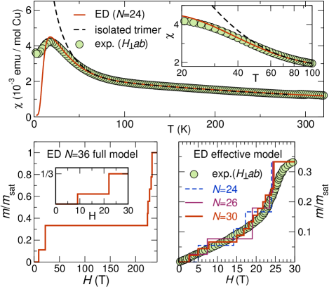
Figure 3: (Color online) Top: magnetic susceptibility of the microscopic spin Hamiltonian calculated by ED on a $N$ = 24 site lattice compared to experiment (Ref. Ishikawa (private communication)) and an isolated trimer model. Bottom left: GS magnetization curve simulated on a lattice of $N$=36 spins for the same model. Insets are magnifications of the respective data. Bottom right: GS magnetization of the full effective model sup with $N$ = 24, 26, and 30 pseudospins compared to experiment (Ref. Ishikawa et al. (2015)).

After establishing good agreement with the $\chi(T)$ data, we employ a larger lattice of $N$ = 36 spins and calculate the GS magnetization curve, which shows a wide $\frac{1}{3}$-magnetization plateau between the critical fields $H_{\text{c1}}$ and $H_{\text{c2}}$ (Fig. 3, bottom left). Scaling with $J$ and $g$ from the $\chi(T)$ fit, without any adjustable parameters, yields $H_{\text{c1}}$ = 22 T in agreement with the experimental $H_{\text{c1}}$ = 26 T. In the plateau phase, first- and second-neighbor spin correlations within each trimer amount to $\langle{\bf S}_{0}{}\cdot{\bf S}_{1}\rangle$ $\equiv$ $\langle{\bf S}_{1}{}\cdot{\bf S}_{2}\rangle$ = $-0.4938$ and $\langle{\bf S}_{0}{}\cdot{\bf S}_{2}\rangle$ = 0.2470, very close to the isolated trimer result ($-\frac{1}{2}$ and $\frac{1}{4}$, respectively sup ). Hence, the $\frac{1}{3}$-plateau phase can be approximated by a product of polarized spin trimers formed by strong $J$ bonds (Fig. 1, right), and thus is very different from the plateau phases of the KHM (Fig. 1, left) and the CFC model (Fig. 1, middle). The plateau stretches up to a remarkably high $H_{\text{c2}}$ $\simeq$ 225 T, at which the spin trimers break up, allowing the magnetization to triple.

ED-simulated spin correlations indicate that the simplest effective model — the isolated trimer model — already captures the nature of this plateau phase. On general grounds, we can expect the isolated trimer model to be valid only at high temperatures. However, it provides a surprisingly good fit for magnetic susceptibility down to 60 K (Fig. 3, top), i.e. at a much weaker energy scale than the leading exchange $J$ $\simeq$ 250 K (Fig. 3). This motivates us to treat the inter-trimer couplings perturbatively and derive a more elaborate effective model valid at low temperatures and in low fields ($T,g\mu_{\text{B}}H/k_{\text{B}}\ll J$).

To this end, we adopt the lowest-energy doublet of each trimer at $H$ = 0 as the basis for a pseudospin-$\frac{1}{2}$ operator $\mathbf{T}_{i}$. The $\frac{1}{3}$-plateau phase corresponds to the full polarization of pseudospin-$\frac{1}{2}$ moments ($m_{\mathrm{sat}}^{\mathrm{eff}}$ = $m_{\mathrm{sat}}/3$). Degenerate perturbation theory to second order in the inter-trimer couplings yields an effective Heisenberg model on a triangular lattice with spatially anisotropic nearest-neighbor couplings ${\cal J}_{1}$ = $-34.9$ K and ${\cal J}_{2}$ = 36.5 K and much weaker longer-range couplings such as ${\cal J}_{2}^{\prime}$ = 6.8 K and ${\cal J}_{3}$ = 4.6 K shown in Fig. 2 (d) sup . The competition between FM ${\cal J}_{1}$ and AF ${\cal J}_{2}$ underlies the frustrated nature of the effective model. Larger finite lattices available to ED of the effective model allow us to amend the critical field $H_{\mathrm{c1}}$ estimate compared to the full microscopic model (Fig. 3, bottom left) and reproduce a pronounced change in the $M(H)$ slope (Fig. 3, bottom right), which agrees with the experimental kink at $\sim$22 T Ishikawa et al. (2015).

Effective models provide important insights into the nature of field-induced states. Recent NMR experiments on single crystals revealed the emergence of the incommensurate collinear spin-density-wave (SDW) phase “II” ($H$ $<$ 23 T) and the “N” phase preceding the plateau (23 T $<$ $H$ $<$ 26 T) Ishikawa et al. (2015). We first address the nature of the latter phase, by treating the fully-polarized pseudospin state (the 1/3-plateau state of volborthite) as the vacuum and analyzing the magnon instabilities to it.

To this end, we resort to a model with three leading effective couplings ${\cal J}_{1}$, ${\cal J}_{2}$, and ${\cal J}_{2}^{\prime}$. This model is equivalent to the frustrated FM square lattice model, where a bond nematic order emerges owing to condensation of two-magnon bound states (bimagnons) for ${\cal J}_{2}={\cal J}_{2}^{\prime}\gtrsim 0.4|{\cal J}_{1}|$ Shannon et al. (2006). Here we take the approximate ratio ${\cal J}_{2}/|{\cal J}_{1}|$ = 1 of the perturbative estimates, and study the influence of ${\cal J}_{2}^{\prime}$ on the ground state. We find that the bond nematic order is robust for ${\cal J}_{2}^{\prime}/|{\cal J}_{1}|\gtrsim 0.3$ sup , as signaled by the occurrence of bimagnon condensation at $H_{\mathrm{c1}}^{(2)}$, at which the plateau state is already destabilized, but before single-magnon condensation sets in at $H_{\mathrm{c1}}^{(1)}$ (Fig. 4, a). The bond nematic phase shows no long-range magnetic order besides the field-induced moment, but it is characterized by a bond order with an alternating sign of directors $D_{ij}\equiv\langle{}T^{x}_{i}T^{x}_{j}-T^{y}_{i}T^{y}_{j}\rangle$ residing on ${\cal J}_{1}$ bonds (Fig. 4, b) foo . This phase is a viable candidate for the experimentally observed “N” phase, whose NMR spectra are not explained by simple magnetic orders Ishikawa et al. (2015).

While bimagnons are stable in a wide region of the ${\cal J}_{1}$-${\cal J}_{2}$-${\cal J}_{2}^{\prime}$ model, longer-range effective couplings such as ${\cal J}_{3}$ tend to destabilize bimagnons. However, a slight tuning of the microscopic model (e.g., increasing of $|J^{\prime}|$) can counteract this effect, thereby recovering the nematic phase sup . Long-range effective couplings are also sensitive to weak long-range exchanges neglected in the full microscopic model. In the absence of experimental estimates for these small exchanges, the ${\cal J}_{1}$-${\cal J}_{2}$-${\cal J}_{2}^{\prime}$ effective model is an adequate approximation, which allows us to study the nature of the field-induced phases in volborthite.

Below 23 T, NMR spectra indicate the onset of an incommensurate collinear phase “II” Ishikawa et al. (2015). Unfortunately, incommensurate spin correlations produce irregular finite-size effects that impede an ED simulation. Yet, on a qualitative level, further truncation of the model to the effective couplings ${\cal J}_{1}$ and ${\cal J}_{2}$ leads to an anisotropic triangular model, for which a field-theory analysis predicts the SDW order for $m\lesssim\frac{2}{3}m_{\mathrm{sat}}^{\mathrm{eff}}=\frac{2}{9}m_{\mathrm{sat}}$ Starykh et al. (2010).

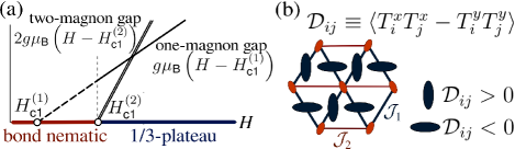
Figure 4: (Color online) (a) The behavior of one- and two-magnon gaps in the $\frac{1}{3}$-plateau phase, which gives rise to a bond nematic phase. (b) Schematic picture of the bond nematic phase in the effective model. Orientation of dark ellipses represents the sign of directors $\mathcal{D}_{ij}$ on ${\cal J}_{1}$ bonds foo .

Next, we go a step beyond the Heisenberg model and consider antisymmetric Dzyaloshinskii-Moriya (DM) components for the leading couplings $J$ and $J_{1}$. By performing noncollinear DFT+$U$ calculations with vasp Kresse and Furthmüller (1996a); *VASP_2, we obtain $|D_{1}|/J_{1}$ $\simeq$ 0.12 with $\vec{D}_{1}$ nearly orthogonal to the frustrated chains. DM vectors $\vec{D}$ within the trimers are nearly orthogonal to the respective interatomic vectors and amount to $|D|$/$J$ $\simeq$ 0.09 sup . We analyzed the influence of $D$ for isolated dimers with ED and found a minute change in spin correlations in the plateau state, which amounts to 2 $\%$ at most. However, these DM interactions are the leading anisotropy at low fields, and can give rise to the two consecutive transitions to the incommensurate phase “I” ($T$ $<$ 1 K, $H$ $<$ 4 T) Yoshida et al. (2012).

Finally, we address the intriguing question why the $\frac{1}{3}$ plateau has not been observed in powder samples. We remind the reader that the trimers are underlain by the stretching distortion of Cu(1)O₆ octahedra, which selects two out of four neighboring VO₄ octahedra for the $J$ superexchange pathway (Fig. 2, b). In single crystals, the distortion axes are fixed, and the trimers form an ordered parquet-like pattern. Powder samples on the other hand are more prone to a random choice of the distortion axis. A single defect of this type permutes $J$ and $J^{\prime}$, ruining the trimer picture locally. This tentative scenario explains the absence of a plateau and the strong dependence on the sample quality in the powder magnetization data.

In summary, the stretching distortion of the magnetic Cu(1)O₆ octahedra in volborthite leads to the model of coupled trimers, very different from the anisotropic kagome and coupled frustrated chain models discussed in earlier studies. Based on DFT calculations and ED simulations, we conclude that i) the microscopic magnetic model of volborthite contains four exchanges with a ratio $J$:$J^{\prime}$:$J_{1}$:$J_{2}$ = 1:$-0.2$:$-0.5$:0.2 and $J$ = 252 K; ii) the $\frac{1}{3}$-magnetization plateau can be understood as a product of nearly independent polarized trimers, and iii) the effective ${\cal J}_{1}$-${\cal J}_{2}$-${\cal J}_{2}^{\prime}$ model shows indications for a bond nematic phase which precedes the onset of the plateau.

Note added: A recent NMR study Yoshida et al. supports our bond nematic phase scenario below the $\frac{1}{3}$-plateau.

Table S1: Comparison of total energies yielded by nonmagnetic DFT calculations using the full-potential code fplo version 9.07-41 S:FPLO . The respective references, experimental method (XRD for x-ray diffraction, ND for neutron diffraction), number of formula units in the unit cell ($Z$), the space group and the $k$-mesh are given in columns 1-5. $E^{\text{GGA}}$ and $E^{\text{LDA}}$ correspond to the total energies obtained using parameterizations for the exchange and correlation potential from Refs. S:PBE96 and S:PW92 , respectively. The hydrogen positions are optimized with respect to total energy, the resulting forces are below 0.01 eV/Å.

reference	method	$Z$	sp. gr.	$k$-mesh	$E^{\text{GGA}}/Z$ (Hartree)	$E^{\text{LDA}}/Z$ (Hartree)
Ref. S:volb:basso88	XRD	1	$C2/m$	8$\times$8$\times$8	$-7695.23828$	$-7678.79575$
Ref. S:volb:lafontaine90	ND	1	$C2/m$	8$\times$8$\times$8	$-7695.24387$	$-7678.80053$
Ref. S:volb:lafontaine90	XRD	1	$C2/m$	8$\times$8$\times$8	$-7695.22987$	$-7678.79266$
Ref. S:volb:kashaev08	XRD	2	$CC$	4$\times$4$\times$4	$-7695.24642$	$-7678.80498$
Ref. S:volb:yoshida12ncomm	XRD, 150 K	2	$C2/c$	4$\times$4$\times$4	$-7695.24236$	$-7678.80240$
Ref. S:volb:yoshida12ncomm	XRD, 322 K	1	$C2/m$	8$\times$8$\times$8	$-7695.23947$	$-7678.79349$
Ref. S:volb:ishikawa12	XRD	2	$C2/c$	4$\times$4$\times$4	$-7695.24878$	$-7678.80835$
Ref. S:volb:ishikawa15	XRD	4	$P2_{1}/c$	4$\times$4$\times$4	$-7695.25191$	$-7678.81252$

Table S2: Crystal structure used for DFT and DFT+$U$ calculations. We use the 50 K data from Ref. S:volb:ishikawa15 in the conventional setup, i.e. the space group is $P2_{1}/c$ (14), $a$ = 14.41 Å, $b$ = 5.8415 Å, $c$ = 10.6489 Å, and $\beta$ = 95.586^∘. The hydrogen coordinates shown bold are optimized within GGA+$U$. All other atomic coordinates are taken from Ref. S:volb:ishikawa15 .

atom	Wyckoff position	$x/a$	$y/b$	$z/c$
Cu1	2$d$	$\frac{1}{2}$	0	$\frac{1}{2}$
Cu2	2$c$	0	0	$\frac{1}{2}$
Cu3	4$e$	0.00233	0.75600	0.24626
Cu4	4$e$	0.49930	0.74625	0.25280
V1	4$e$	0.12660	0.52334	0.49667
V2	4$e$	0.37297	$-0.02131$	0.00304
O1	4$e$	0.24991	$-0.04890$	0.00158
O2	4$e$	0.05938	0.00418	0.34368
H1	4$e$	0.12961	0.01212	0.34767
O3	4$e$	0.55895	$-0.00105$	0.34372
H2	4$e$	0.62959	0.00012	0.34817
O4	4$e$	0.07440	0.50571	0.34159
O5	4$e$	0.42524	$-0.00532$	0.15831
O6	4$e$	0.26060	0.50190	0.17836
O7	4$e$	0.24083	0.03230	0.31923
O8	4$e$	0.09912	0.20580	0.07522
O9	4$e$	0.60273	0.78700	0.07584
O10	4$e$	0.08846	0.73814	0.07118
O11	4$e$	0.41442	0.75383	0.42937
H3	4$e$	0.20595	0.56499	0.12695
H4	4$e$	0.23942	0.35162	0.20575
H5	4$e$	0.26676	0.88701	0.29281
H6	4$e$	0.29312	0.10203	0.37325

Table S3: Comparison of transfer integrals $t_{ij}$ (meV) evaluated using Wannier functions for one-orbital ($x^{2}-y^{2}$, only) and two-orbital ($x^{2}-y^{2}$ and $3z^{2}-r^{2}$) models. For the latter, only the transfer integrals between the half-filled $x^{2}-y^{2}$ are provided. The respective band dispersions are shown in Fig. 3 and Fig. S1. Direct Cu..Cu distances $d_{\text{Cu..Cu}}$ are given in Å).

transfer integral	$d_{\text{Cu..Cu}}$	$t$ for one-orbital WFs	$t$ for two-orbital WFs ($x^{2}-y^{2}\leftrightarrow{}x^{2}-y^{2}$)
$t$	3.053 / 3.058	$-191$ / $-194$	$-198$ / $-195$
$t^{\prime}$	3.016 / 3.020	$-80$ / $-84$	$-80$ / $-85$
$t_{1}$	2.922 / 2.923	$-98$ / $-100$	$-98$ / $-100$
$t_{2}$	5.842 / 5.842	64 / 64	66 / 66

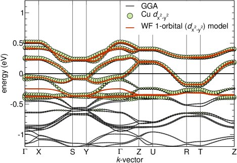
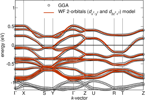
Figure S1: (Color online) Left: GGA band structure of volborthite (solid lines) with band characters for the Cu $d_{x^{2}-y^{2}}$ orbitals. The dashed line indicates the projection onto Cu-centered Wannier functions (WFs) within a one-orbital $x^{2}-y^{2}$ model. Note the deviations around $\sim$$-$0.4 eV. Right: The deviations around $\sim$$-$0.4 eV are remedied in a two-orbital ($x^{2}-y^{2}$ and $3z^{2}-r^{2}$) model. The $k$-points are: $\Gamma$ = $\left(000\right)$, X = $\left(\frac{\pi}{a}00\right)$, M = $\left(\frac{\pi}{a}\frac{\pi}{b}0\right)$, Y = $\left(0\frac{\pi}{b}0\right)$, Z = $\left(00\frac{\pi}{c}\right)$, XZ = $\left(\frac{\pi}{a}0\frac{\pi}{c}\right)$, MZ = $\left(\frac{\pi}{a}\frac{\pi}{b}\frac{\pi}{c}\right)$, and YZ = $\left(0\frac{\pi}{b}\frac{\pi}{c}\right)$.

I Effective Hamiltonians

In the main text, we analyze the physics at low temperatures and low fields ($T,h\equiv g\mu_{B}H/k_{B}\ll J$) by using an effective Hamiltonian of pseudospin-$\frac{1}{2}$ moments living on trimers. Here we describe details of the derivation of this effective Hamiltonian and our analyses of the magnon spectra and the magnetization process of this model. We also derive yet another low-temperature effective Hamiltonian suitable for high fields ($T,|h-3J/2|\ll J$), which can be used to determine the high-field end $H_{\mathrm{c2}}$ of the plateau phase and the saturation field $H_{\mathrm{c3}}$.

Our use of these effective Hamiltonians is motivated by the distinct hierarchy of the exchange couplings $J>|J_{1}|>J_{2},|J^{\prime}|$ revealed in DFT+$U$. We start from the limit of large $J$, where the system decouples into trimers. In this limit, each isolated trimer exhibits a wide $\frac{1}{3}$-magnetization plateau over $0<h<3J/2$. At each endpoint of the plateau, where a level crossing occurs in the ground state of each trimer, the total system possesses a macroscopic degeneracy and is highly susceptible to inter-trimer couplings. Our effective Hamiltonian is derived around each endpoint by performing degenerate perturbation theory in terms of $J^{\prime}$, $J_{1}$, and $J_{2}$. This kind of approach is known as strong coupling expansion S:Mila11S , and is often used to analyze quantum spin systems with coupled cluster structures such as coupled dimers S:Mila11S ; S:Totsuka98S ; S:Mila98S and coupled trimers S:Tonegawa00S ; S:Honecker01S . Our derivation of the effective Hamiltonians goes essentially in parallel with Refs. S:Tonegawa00S ; S:Honecker01S .

I.1 Isolated trimer

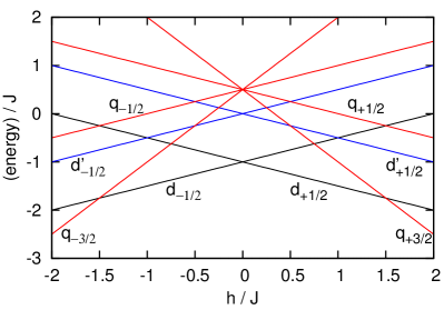
Figure S2: The spectrum of an isolated trimer Hamiltonian (1) as a function of the magnetic field $h$. The eigenstates and eigenenergies are shown in Eqs. (2) and (3), respectively.

We first consider an isolated trimer Hamiltonian

$$H_{012}=J(\bm{S}_{0}\cdot\ \bm{S}_{1}+\bm{S}_{1}\cdot\bm{S}_{2})-h\sum_{j=0}^{2}S^{z}_{j},$$ (1)

where $\bm{S}_{1}$ and $\bm{S}_{0,2}$ are the spin-$\frac{1}{2}$ operators at the central and other sites of the trimer, respectively. At $h=0$, because of the SU(2) symmetry and the parity symmetry around the site $1$, the eigenstates are classified into the quadruplet $\{|q_{\mu}\rangle\}$, the even-parity doublet $\{|d_{\mu}\rangle\}$, and the odd-parity doublet $\{|d^{\prime}_{\mu}\rangle\}$, where $\mu$ is the eigenvalue of $\sum_{j=0}^{2}S_{j}^{z}$. Their wave functions for $\mu>0$ are given by

$$\begin{split}|q_{+\frac{3}{2}}\rangle&=|\uparrow\uparrow\uparrow\rangle,\\ |q_{+\frac{1}{2}}\rangle&=\frac{1}{\sqrt{3}}\left(|\uparrow\uparrow\downarrow\rangle+|\downarrow\uparrow\uparrow\rangle+|\uparrow\downarrow\uparrow\rangle\right),\\ |d_{+\frac{1}{2}}\rangle&=\frac{1}{\sqrt{6}}\left(|\uparrow\uparrow\downarrow\rangle+|\downarrow\uparrow\uparrow\rangle-2|\uparrow\downarrow\uparrow\rangle\right),\\ |d^{\prime}_{+\frac{1}{2}}\rangle&=\frac{1}{\sqrt{2}}\left(|\uparrow\uparrow\downarrow\rangle-|\downarrow\uparrow\uparrow\rangle\right).\end{split}$$ (2)

Other eigenstates with $\mu<0$ are obtained by applying the spin reversal to the above. The Zeeman term in Eq. (1) commutes with the Heisenberg terms, and only shifts the eigenenergies by $-h\mu$. The eigenenergies in the presence of a field $h$ are calculated as

$$\begin{split}|q_{\mu}\rangle:&~{}\frac{1}{2}J-h\mu;\\ |d_{\mu}\rangle:&~{}-J-h\mu;\\ |d_{\mu}^{\prime}\rangle:&~{}-h\mu,\end{split}$$ (3)

which are plotted in Fig. S2. At $h=0$, the ground states are the even-parity doublet $|d_{\pm\frac{1}{2}}\rangle$; they are split for $h\neq 0$. At $h=3J/2$, a level crossing occurs, and the ground state is replaced by the fully polarized state $|q_{+\frac{3}{2}}\rangle$. This level structure gives a wide magnetization plateau with $m/m_{\mathrm{sat}}=1/3$ over $0<h<3J/2$. At the level crossing points $h=0$ and $3J/2$, the total system consisting of $N_{\mathrm{t}}$ trimers possesses a macroscopic degeneracy $2^{N_{\mathrm{t}}}$ of ground states. We restrict ourselves to this degenerate manifold, and analyze the splitting of the degeneracy due to inter-trimer couplings by deriving effective Hamiltonians.

The small Hilbert space of the isolated trimer model facilitates a direct evaluation of its partition function, and hence its magnetic susceptibility, which is given by:

$$\chi^{*}(\beta)=\beta\left(\frac{1}{12}+\frac{2}{3}\left({2+\exp{\frac{\beta}{2}}\ +\exp{\frac{3\beta}{2}}}\right)^{-1}\right),$$ (4)

where $\beta$ is the inverse temperature.

I.2 Effective Hamiltonian for $|m/m_{\rm sat}|\leq 1/3$

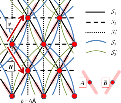
Figure S3: Effective Heisenberg Hamiltonain for $|h|\ll J$. The five largest couplings obtained in the second-order perturbation theory are displayed. For each trimer indicated by a light red bar (with its center at ${\bm{r}}$) , we introduce a pseudospin-$\frac{1}{2}$ operator $\bm{T}_{\bm{r}}$. These pseudospins form a triangular lattice. This lattice consists of two sublattices $A$ and $B$ corresponding to two different directions of trimers. The vectors $\bm{u}$ and $\bm{v}$ (of lengths $|\bm{u}|,|\bm{v}|\simeq b\simeq 6\AA$) connect between neighboring sites on the triangular lattice.

Table S4: Nonzero coupling constants ${\cal J}_{\Delta{\bm{r}},X}$ in the effective Hamiltonian (7). The vectors $\bm{u}$ and $\bm{v}$ are defined in Fig. S3. Only for ${\cal J}_{3}$ and ${\cal J}_{3}^{\prime}$, the relative vector $\Delta{\bm{r}}$ depends on the sublattice $X$, as indicated in the corresponding rows. The first- and second-order perturbative estimates (third and fourth columns) are calculated by substituting Eq. (9) into Eqs (6) and (8). We also consider Models I and II shown in the fifth and sixth columns, where the leading three and four couplings in the second-order model are taken into account, respectively; these simplified models help to understand the essential physics arising from the leading couplings. For each of these models, one- and two-magnon condensation points, $h_{\mathrm{c1}}^{(n)}=g\mu_{B}H_{\mathrm{c1}}^{(n)}/k_{B}$ with $n=1,2$, are presented. Here, $g=2.151$ obtained in the main text is used to convert $h_{\mathrm{c1}}^{(n)}$ into $H_{\mathrm{c1}}^{(n)}$. In the four models, the one-magnon spectrum has the minimum at incommensurate wave vectors ${\bm{k}}b=\pm(Q,0)$, and the value of $Q/(2\pi)$ is also presented.

	relative vectors $\Delta{\bm{r}}$	1st-order	2nd-order	Model I	Model II
${\cal J}_{1}$	$\bm{u},\bm{v}$	$-44.8$ K	$-34.9$ K	$-34.9$ K	$-34.9$ K
${\cal J}_{2}$	$\bm{u}+\bm{v}$	44.8 K	36.5 K	36.5 K	36.5 K
${\cal J}_{2}^{\prime}$	$-\bm{u}+\bm{v}$		6.8 K	6.8 K	6.8 K
${\cal J}_{3}$	$(2\bm{u},A),~{}(2\bm{v},B)$		4.6 K		4.6 K
${\cal J}_{3}^{\prime}$	$(2\bm{v},A),~{}(2\bm{u},B)$		1.7 K
${\cal J}_{4}$	$2\bm{u}+\bm{v},\bm{u}+2\bm{u}$		1.7 K
${\cal J}_{5}$	$2(\bm{u}+\bm{v})$		$-1.3$ K
$h_{\mathrm{c1}}^{(1)}~{}(H_{\mathrm{c1}}^{(1)})$		22.4 K (15.5 T)	35.0 K (24.2 T)	19.9 K (13.8 T)	27.2 K (18.9 T)
$Q/(2\pi)$		0.333	0.370	0.341	0.360
$h_{\mathrm{c1}}^{(2)}~{}(H_{\mathrm{c1}}^{(2)})$		22.4 K (15.5 T)	35.0 K (24.2 T)	25.7 K (17.8 T)	29.0 K (20.1 T)

Here we derive the effective Hamiltonian for the range $|m/m_{\rm sat}|\leq 1/3$. We label each trimer by the position ${\bm{r}}$ of its central site. These positions form a triangular lattice as shown in Fig. S3. This lattice consists of two sublattices $A$ and $B$ corresponding to two different directions of trimers.

For $|h|\ll J$, we use the lowest-energy doublet $|d_{\pm\frac{1}{2}}\rangle_{\bm{r}}$ at $h=0$ as the local basis on each trimer ${\bm{r}}$. Using these states, we introduce a pseudospin-$\frac{1}{2}$ operator

$$\bm{T}_{\bm{r}}=\left(|d_{+\frac{1}{2}}\rangle_{\bm{r}},|d_{-\frac{1}{2}}\rangle_{\bm{r}}\right)\frac{\bm{\sigma}}{2}\begin{pmatrix}{}_{\bm{r}}\langle d_{+\frac{1}{2}}|\\ {}_{\bm{r}}\langle d_{-\frac{1}{2}}|\end{pmatrix},$$ (5)

where $\bm{\sigma}=(\sigma^{x},\sigma^{y},\sigma^{z})$ are the Pauli matrices.

The first-order effective Hamiltonian is derived by projecting the inter-trimer interactions onto the degenerate manifold $V_{0}=\bigotimes_{\bm{r}}\mathrm{Span}(\{|d_{\pm\frac{1}{2}}\rangle_{\bm{r}}\})$. The obtained Hamiltonian is a Heisenberg model of pseudospins $\{\bm{T}_{\bm{r}}\}$ on the triangular lattice with spatially anisotropic nearest-neighbor couplings

$${\cal J}_{1}^{\rm(1st)}=\frac{2}{9}(2J_{1}-J^{\prime}),~{}~{}{\cal J}_{2}^{\rm(1st)}=\frac{8}{9}J_{2},$$ (6)

as shown in Fig. S3.

To calculate the second-order effective Hamiltonian, we take into account various processes where a state in $V_{0}$ is virtually promoted to an excited state outside $V_{0}$, and then comes back to $V_{0}$ by the operations of the inter-trimer interactions. Such virtual processes give rise to various further-neighbor interactions between pseudospins. The resulting Hamiltonian is a Heisenberg model

$$H_{\mathrm{eff}}=\sum_{\bm{r}}\sum_{\Delta{\bm{r}}}{\cal J}_{\Delta{\bm{r}},X_{\bm{r}}}\bm{T}_{\bm{r}}\cdot\bm{T}_{{\bm{r}}+\Delta{\bm{r}}}-h\sum_{{\bm{r}}}T^{z}_{\bm{r}},$$ (7)

where $X_{\bm{r}}=A,B$ indicates the sublattice which ${\bm{r}}$ belongs to. The coupling constants ${\cal J}_{\Delta{\bm{r}},X}$ show seven nonzero different values as listed in Table S4, and their second-order expressions are given by

$$\begin{split}{\cal J}_{1}^{\rm(2nd)}=&\frac{2}{9}(2J_{1}-J^{\prime})+\frac{211{J_{1}}^{2}+48J_{1}J^{\prime}-118{J^{\prime}}^{2}}{1620J}\\ &+\frac{8J_{2}(-4J_{1}+5J^{\prime})}{243J},\\ {\cal J}_{2}^{\rm(2nd)}=&\frac{8}{9}J_{2}-\frac{{J_{2}}^{2}}{81J}-\frac{2(-2J_{1}+J^{\prime})(-13J_{1}+8J^{\prime})}{243J},\\ {\cal J}_{2}^{\prime{\rm(2nd)}}=&\frac{2(-2J_{1}+J^{\prime})(-5J_{1}-8J^{\prime})}{243J},\\ {\cal J}_{3}^{\rm(2nd)}=&\frac{2(-5J_{1}+4J^{\prime})(-J_{1}-4J^{\prime})}{243J},\\ {\cal J}_{3}^{\prime{\rm(2nd)}}=&\frac{5(-2J_{1}+J^{\prime})^{2}}{486J},\\ {\cal J}_{4}^{\rm(2nd)}=&\frac{8J_{2}(-4J_{1}+5J^{\prime})}{243J},\\ {\cal J}_{5}^{\rm(2nd)}=&-\frac{32{J_{2}}^{2}}{243J}.\end{split}$$ (8)

Most of these interactions do not depend on the sublattice $X$, and have the translational invariance of the triangular lattice. Only ${\cal J}_{3}$ and ${\cal J}^{\prime}_{3}$ depend on the sublattice $X$, and double the unit cell of the effective model when ${\cal J}_{3}\neq{\cal J}_{3}^{\prime}$; the primitive vectors of the system then change to $\pm\bm{u}+\bm{v}$. Using

$$J:J^{\prime}:J_{1}:J_{2}=1:-0.2:-0.5:0.2,~{}~{}J\simeq 252~{}\mathrm{K},$$ (9)

obtained in the main text, the effective coupling constants are calculated as in the columns “1st-order” and “2nd-order” in Table S4. The five largest couplings in the second-order model are displayed in Fig. S3.

I.3 Magnon spectra

Using the effective model $H_{\mathrm{eff}}$ in Eq. (7), we here calculate the spectra of one- and two-magnon excitations which lower the total magnetization by one and two, respectively, from the $\frac{1}{3}$-magnetization plateau state. The plateau state corresponds to the fully polarized state of pseudospins $\bigotimes_{\bm{r}}|d_{+\frac{1}{2}}\rangle_{\bm{r}}=:|\mathrm{vac}\rangle$, which we view as the magnon vacuum in the following. Then, $T^{\pm}_{\bm{r}}:=T^{x}_{\bm{r}}\pm iT^{y}_{\bm{r}}$ play the roles of magnon annihilation and creation operators, and the magnon occupation number at the site ${\bm{r}}$ is given by $n_{\bm{r}}:=\frac{1}{2}-T_{\bm{r}}^{z}$. Using these operators, the Hamiltonian is rewritten as

$$H_{\mathrm{eff}}=N_{\mathrm{t}}\left(\frac{1}{4}{\cal J}-\frac{h}{2}\right)+h\sum_{\bm{r}}n_{\bm{r}}+H_{\mathrm{mag}},$$ (10)

where

$${\cal J} =\frac{1}{N_{\mathrm{t}}}\sum_{\bm{r}}\sum_{\Delta{\bm{r}}}{\cal J}_{\Delta{\bm{r}},X_{\bm{r}}}$$

$$=2{\cal J}_{1}+{\cal J}_{2}+{\cal J}_{2}^{\prime}+{\cal J}_{3}+{\cal J}_{3}^{\prime}+2{\cal J}_{4}+{\cal J}_{5},$$ (11)

$$H_{\mathrm{mag}} =-{\cal J}\sum_{\bm{r}}n_{\bm{r}}$$

$$+\sum_{\bm{r}}\sum_{\Delta{\bm{r}}}{\cal J}_{\Delta{\bm{r}},X_{\bm{r}}}\left[\frac{1}{2}\left(T^{+}_{\bm{r}}T^{-}_{{\bm{r}}+\Delta{\bm{r}}}+\mathrm{h.c.}\right)+n_{\bm{r}}n_{{\bm{r}}+\Delta{\bm{r}}}\right].$$ (12)

The first term in Eq. (10) is the energy of the vacuum $|\mathrm{vac}\rangle$. The second term is the Zeeman term, which plays the role of a magnon chemical potential. The third term $H_{\mathrm{mag}}$ contains magnon kinetic and interaction terms, and does not depend on $h$. Below we calculate the $n$-magnon spectrum of $H_{\mathrm{mag}}$, and in particular determine the lowest energy $E^{(n)}$ in it. We then find from Eq. (10) that the minimum energy cost for creating $n$ magnons from the vacuum is given by $E^{(n)}+hn$. This energy reaches zero at $h=h_{\mathrm{c1}}^{(n)}=-E^{(n)}/n$, which corresponds to an $n$-magnon condensation point.

While the second-order effective model is expected to describe well the properties of the original model with Eq. (9) for $T,h\ll J$, it contains small couplings of magnitudes less than $2$ K, which may be influenced easily by potential parameter changes or inclusion of small further-neighbor couplings in the original model, which are not estimated in the DFT+U calculation. We therefore consider also Models I and II shown in Table S4, where the leading three and four couplings in the second-order model are taken into account, respectively. These simplified models help to understand the essential physics arising from the leading effective couplings.

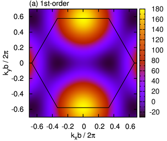
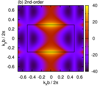
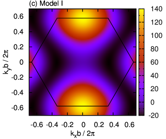
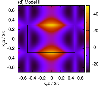
Figure S4: One-magnon spectra of $H_{\mathrm{mag}}$ in Eq. (12) for the four models shown in Table S4. We plot $\epsilon({\bm{k}})$ in Eq. (13) for (a) and (c) , and $\epsilon_{-}({\bm{k}})$ in Eq. (16) for (b) and (d). The color indicates an energy in units of Kelvin. A hexagon or a square indicates the first Brillouin zone. The wave numbers, $k_{x}$ and $k_{y}$, are defined along the horizontal and vertical directions of Fig. S3, respectively.

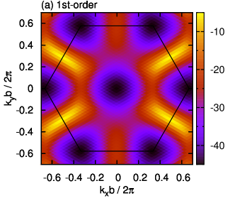
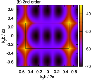
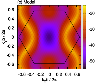
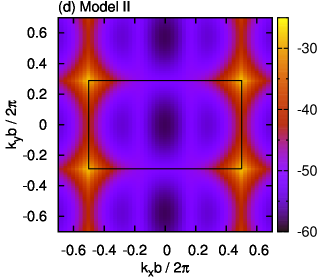
Figure S5: Two-magnon spectra of $H_{\mathrm{mag}}$ in Eq. (12) for the four models shown in Table S4.

We first analyze one-magnon spectra of $H_{\mathrm{mag}}$. When ${\cal J}_{3}={\cal J}_{3}^{\prime}$, the effective model has the translational invariance of the triangular lattice. In this case, one-magnon state forms a single band

$$\epsilon({\bm{k}})=-{\cal J}+\sum_{\Delta{\bm{r}}}{\cal J}_{\Delta{\bm{r}}}\cos({\bm{k}}\cdot\Delta{\bm{r}}).$$ (13)

When ${\cal J}_{3}\neq{\cal J}_{3}^{\prime}$, the unit cell is doubled, and the one-magnon bands are obtained by diagonalizing the $2\times 2$ matrix

$$M({\bm{k}})=\epsilon_{0}({\bm{k}})I+\bm{J}({\bm{k}})\cdot\bm{\sigma},$$ (14)

where $I$ is the identity matrix, and

$$\begin{split}\epsilon_{0}({\bm{k}})&=-{\cal J}+{\cal J}_{2}\cos(k_{u}+k_{v})+{\cal J}_{2}^{\prime}\cos(k_{u}-k_{v})\\ &~{}~{}~{}+\frac{1}{2}({\cal J}_{3}+{\cal J}_{3}^{\prime})\left[\cos(2k_{u})+\cos(2k_{v})\right]\\ &~{}~{}~{}+{\cal J}_{5}\cos(2k_{u}+2k_{v}),\\ J^{x}({\bm{k}})&={\cal J}_{1}\left(\cos k_{u}+\cos k_{v}\right)\\ &~{}~{}~{}+{\cal J}_{4}\left[\cos(2k_{u}+k_{v})+\cos(k_{u}+2k_{v})\right],\\ J^{y}({\bm{k}})&=0,\\ J^{z}({\bm{k}})&=\frac{1}{2}({\cal J}_{3}-{\cal J}_{3}^{\prime})\left[\cos(2k_{u})-\cos(2k_{v})\right]\end{split}$$ (15)

with $k_{u}={\bm{k}}\cdot\bm{u}$ and $k_{v}={\bm{k}}\cdot\bm{v}$. The two bands are calculated as

$$\epsilon_{\pm}({\bm{k}})=\epsilon_{0}({\bm{k}})\pm|\bm{J}({\bm{k}})|.$$ (16)

The (lower) one-magnon band $\epsilon({\bm{k}})$ or $\epsilon_{-}({\bm{k}})$ is plotted for the four models in Fig. S4. In all the cases, the spectrum has the minimum energy $E^{(1)}$ at incommensurate wave vectors ${\bm{k}}b=\pm(Q,0)$. The one-magnon condensation point $h_{\mathrm{c1}}^{(1)}=-E^{(1)}$ and the incommensurate wave number $Q/(2\pi)$ are presented in Table S4. Remarkably, the band $\epsilon({\bm{k}})$ for Model I shows a line of nearly degenerate minima extending roughly along the vertical direction. This implies suppression of magnon hopping (and hence relative enhancement of magnon interactions) along this direction.

We next analyze two-magnon spectra. To this end, we introduce the two-magnon basis S:Kecke07S , which is given by

$$|\Delta{\bm{r}},{\bm{k}}\rangle=\frac{1}{\sqrt{N_{\mathrm{t}}}}\sum_{\bm{r}}e^{i{\bm{k}}\cdot{\bm{r}}}T^{-}_{\bm{r}}T^{-}_{{\bm{r}}+\Delta{\bm{r}}}|\mathrm{vac}\rangle$$ (17)

when ${\cal J}_{3}={\cal J}_{3}^{\prime}$, and by

$$|X,\Delta{\bm{r}},{\bm{k}}\rangle=\frac{1}{\sqrt{N_{\mathrm{t}}/2}}\sum_{{\bm{r}}\in X}e^{i{\bm{k}}\cdot{\bm{r}}}T^{-}_{\bm{r}}T^{-}_{{\bm{r}}+\Delta{\bm{r}}}|\mathrm{vac}\rangle$$ (18)

with $X=A,B$ when ${\cal J}_{3}\neq{\cal J}_{3}^{\prime}$. Here, the magnon relative vector $\Delta{\bm{r}}$ is chosen in the range $|\Delta{\bm{r}}|/b\lesssim O(10^{2})$ in such a way that the double counting of $\pm\Delta{\bm{r}}$ which lead to the same state is avoided. The matrix elements of $H_{\mathrm{mag}}$ are given by

$$\langle\Delta{\bm{r}},{\bm{k}}|H_{\mathrm{mag}}|\Delta{\bm{r}}^{\prime},{\bm{k}}\rangle$$

$$=\sum_{\bm{r}}e^{i{\bm{k}}\cdot{\bm{r}}}\langle\mathrm{vac}|T_{\bm{0}}^{+}T_{\Delta{\bm{r}}}^{+}H_{\mathrm{mag}}T_{\bm{r}}^{-}T_{{\bm{r}}+\Delta{\bm{r}}^{\prime}}^{-}|\mathrm{vac}\rangle,$$ (19)

$$\langle X,\Delta{\bm{r}},{\bm{k}}|H_{\mathrm{mag}}|X^{\prime},\Delta{\bm{r}}^{\prime},{\bm{k}}\rangle$$

$$=\sum_{{\bm{r}}\in X^{\prime}}e^{i{\bm{k}}\cdot({\bm{r}}-\bm{u}\delta_{XB})}$$

$$~{}~{}~{}~{}\times\langle\mathrm{vac}|T_{\bm{u}\delta_{XB}}^{+}T_{\bm{u}\delta_{XB}+\Delta{\bm{r}}}^{+}H_{\mathrm{mag}}T_{\bm{r}}^{-}T_{{\bm{r}}+\Delta{\bm{r}}^{\prime}}^{-}|\mathrm{vac}\rangle$$ (20)

for the bases in Eqs. (17) and (18), respectively. We note that the dependence on $N_{\mathrm{t}}$ has dropped in these expressions, and we are effectively treating an infinite system (an error can only arise from the finite cutoff for $|\Delta{\bm{r}}|$). By performing Lanczos diagonalization for such matrices, we have calculated the lowest eigenenergy for each ${\bm{k}}$, which is plotted in Fig. S5. In (a) the first-order and (b) second-order models, we find nearly degenerate minima at ${\bm{k}}b=(0,0)$ and $\pm(2Q,0)$ with energy $E^{(2)}\approx 2E^{(1)}$; these can be interpreted as two independent magnons, each with the one-magnon lowest energy $E^{(1)}$. In (c) Model I and (d) Model II, by contrast, a single minimum at ${\bm{k}}b=(0,0)$ with energy $E^{(2)}<2E^{(1)}$ is formed, implying a significant effect of attractive interactions. In (c) Model I, in particular, two magnons acquire an appreciable binding energy $2E^{(1)}-E^{(2)}=11.6$ K, which is likely to be due to aforementioned suppression of magnon hopping along the vertical direction. The two-magnon condensation point $h_{\mathrm{c1}}^{(2)}=-E^{(2)}/2$ is presented in Table S4. The relation $h_{\mathrm{c1}}^{(1)}<h_{\mathrm{c1}}^{(2)}$ seen in Models I and II indicates that bimagnon condensation leading to a bond nematic order occurs with lowering the field $h$ from the plateau phase. We have also calculated $3$- and $4$-magnon spectra (not shown), finding no indication of multimagnon condensation with $h_{\mathrm{c1}}^{(n)}>h_{\mathrm{c1}}^{(1)},h_{\mathrm{c1}}^{(2)}~{}(n=3,4)$.

I.4 Exact diagonalization

In the main text, we present the exact diagonalization result for the magnetization process of the second-order effective model in Eq. (7). Here we explain the cluster shapes used for this study. A finite-size cluster is specified by two vectors $\bm{L}_{j}=L_{uj}\bm{u}+L_{vj}\bm{v}$ [$j=1,2;~{}L_{uj},(L_{uj}+L_{vj})/2\in\mathbb{Z}$], which set the periodic boundary conditions $\bm{T}_{\bm{r}}\equiv\bm{T}_{{\bm{r}}+\bm{L}_{j}}$. The number of pseudospins in the system is given by $N_{\mathrm{t}}=|L_{u1}L_{v2}-L_{v1}L_{u2}|$. We have used the following clusters specified by $(L_{u1},L_{v1})$ and $(L_{u2},L_{v2})$:

$$\begin{split}&N_{\mathrm{t}}=24:~{}(5,3),~{}(-3,3);\\ &N_{\mathrm{t}}=26:~{}(5,1),(-1,5);\\ &N_{\mathrm{t}}=30:~{}(5,-1),(0,6).\end{split}$$ (21)

The reason for these choices is as follows. In finite-size clusters with periodic boundary conditions, two distinct interactions $\bm{T}_{\bm{r}}\cdot\bm{T}_{{\bm{r}}+\Delta{\bm{r}}}$ and $\bm{T}_{\bm{r}}\cdot\bm{T}_{{\bm{r}}+\Delta{\bm{r}}^{\prime}}$ fall into the identical one if $\Delta{\bm{r}}-\Delta{\bm{r}}^{\prime}=m_{1}\bm{L}_{1}+m_{2}\bm{L}_{2}~{}(m_{1},m_{2}\in\mathbb{Z})$. In the above choices, where $\bm{L}_{1}$ and $\bm{L}_{2}$ are sufficiently long, such a situation can be avoided. Furthermore, $\bm{L}_{1}$ and $\bm{L}_{2}$ form nearly $120^{\circ}$ to each other in the above choices, making the cluster shape as isotropic as possible. For example, $120^{\circ}$ rotation of $(L_{u1},L_{v1})=(5,1)$ gives $(-L_{v1},L_{u1}-L_{v1})=(-1,4)$. However, the latter vector connects between different sublattices, and thus we shift it slightly and set $(L_{u2},L_{v2})=(-1,5)$ to obtain the $N_{\mathrm{t}}=26$ cluster. Exact diagonalization of the effective model was performed using TITPACK ver. 2 S:TITPACK .

I.5 Effective Hamiltonian for $1/3\leq m/m_{\rm sat}\leq 1$

For $|h-3J/2|\ll J$, we can derive yet another effective model valid in the range $1/3\leq m/m_{\rm sat}\leq 1$, by using $|q_{+\frac{3}{2}}\rangle_{\bm{r}}$ and $|d_{+\frac{1}{2}}\rangle_{\bm{r}}$ as the local basis on each trimer ${\bm{r}}$. Using these states, we introduce a pseudospin-$\frac{1}{2}$ operator

$$\tilde{\bm{T}}_{\bm{r}}=\left(|q_{+\frac{3}{2}}\rangle_{\bm{r}},|d_{+\frac{1}{2}}\rangle_{\bm{r}}\right)\frac{\bm{\sigma}}{2}\begin{pmatrix}{}_{\bm{r}}\langle q_{+\frac{3}{2}}|\\ {}_{\bm{r}}\langle d_{+\frac{1}{2}}|\end{pmatrix}.$$ (22)

The all down state of the pseudospins ($\tilde{T}^{z}_{\bm{r}}=-1/2$) corresponds to the $\frac{1}{3}$-magnetization plateau of the original model; the all up state ($\tilde{T}^{z}_{\bm{r}}=+1/2$) corresponds to the saturation. The first-order effective Hamiltonian is derived in a way similar to the previous case, and has the form of an XXZ model on the triangular lattice with spatially anisotropic couplings. The Hamiltonian is given by

$$\begin{split}\tilde{H}_{\mathrm{eff}}=\sum_{\bm{r}}\sum_{\Delta{\bm{r}}}&\bigg{[}{\cal J}_{\Delta{\bm{r}}}^{xy}(\tilde{T}_{\bm{r}}^{x}\tilde{T}_{{\bm{r}}+\Delta{\bm{r}}}^{x}+\tilde{T}_{\bm{r}}^{y}\tilde{T}_{{\bm{r}}+\Delta{\bm{r}}}^{y})\\ &+{\cal J}_{\Delta{\bm{r}}}^{z}\tilde{T}_{\bm{r}}^{z}\tilde{T}_{{\bm{r}}+\Delta{\bm{r}}}^{z}\bigg{]}-\tilde{h}\sum_{{\bm{r}}}\tilde{T}^{z}_{\bm{r}},\end{split}$$ (23)

where

$$\begin{split}&{\cal J}_{1}^{xy}:={\cal J}_{\bm{u}}^{xy}={\cal J}_{\bm{v}}^{xy}=\frac{1}{6}(J_{1}-2J^{\prime}),\\ &{\cal J}_{1}^{z}:={\cal J}_{\bm{u}}^{z}={\cal J}_{\bm{v}}^{z}=\frac{1}{36}(J_{1}+4J^{\prime}),\\ &{\cal J}_{2}^{xy}:={\cal J}_{\bm{u}+\bm{v}}^{xy}=\frac{1}{3}J_{2},\\ &{\cal J}_{2}^{z}:={\cal J}_{\bm{u}+\bm{v}}^{z}=\frac{1}{18}J_{2},\\ &\tilde{h}=h-h_{0},\ \ \ h_{0}=\frac{3}{2}J+\frac{1}{18}(5J_{1}+5J_{2}+11J^{\prime}).\end{split}$$ (24)

Using Eq. (9), the parameters in this model are calculated as

$$\begin{split}&({\cal J}_{1}^{xy},{\cal J}_{1}^{z},{\cal J}_{2}^{xy},{\cal J}_{2}^{z})=(-4.2,-9.1,16.8,2.8)~{}\mathrm{K},\\ &h_{0}=326~{}\mathrm{K}.\end{split}$$ (25)

Because of the spin-reversal symmetry of the XXZ Hamiltonian, the magnetization process of the original model is symmetric about $h=h_{0}$ at this order of perturbation theory.

We determine the saturation field $\tilde{h}_{\mathrm{s}}$ of the effective model (23) by analyzing the single-magnon instability of the saturated state. One-magnon excitation band above the saturated state is calculated as

$$\begin{split}\tilde{\epsilon}({\bm{k}})=&\tilde{h}-2{\cal J}_{1}^{z}-{\cal J}_{2}^{z}+{\cal J}_{1}^{xy}(\cos k_{u}+\cos k_{v})\\ &+{\cal J}_{2}^{xy}\cos(k_{u}+k_{v}).\end{split}$$ (26)

When $0<-{\cal J}_{1}^{xy}<2J_{2}^{xy}$, this has the minimum at ${\bm{k}}b=\pm(Q,0)$ with $Q=2\arccos\frac{|{\cal J}_{1}^{xy}|}{2{\cal J}_{2}^{xy}}$ and the saturation field $\tilde{h}_{\mathrm{s}}$ is determined as the field $\tilde{h}$ at which this minimum reaches zero, hence

$$\tilde{h}_{\mathrm{s}}=2{\cal J}_{1}^{z}+{\cal J}_{2}^{z}+{\cal J}_{2}^{xy}+\frac{({\cal J}_{1}^{xy})^{2}}{2{\cal J}_{2}^{xy}}.$$ (27)

Using Eq. (25), the high-field end $h_{\mathrm{c2}}$ of the plateau and the saturation field $h_{\mathrm{c3}}$ of the original model are calculated as

$$\begin{split}&(h_{\mathrm{c2}},h_{\mathrm{c3}})=(h_{0}-\tilde{h}_{\mathrm{s}},h_{0}+\tilde{h}_{\mathrm{s}})=(324,328)~{}\mathrm{K}\\ &[(H_{\mathrm{c2}},H_{\mathrm{c3}})=(224,227)~{}\mathrm{T}].\end{split}$$ (28)

These fields agree well with the field at which rapid increase of $m/m_{\mathrm{sat}}$ is found in the exact diagonalization result of the original model. This rapid increase in the short field width $H_{\mathrm{c3}}-H_{\mathrm{c2}}=2\tilde{h}_{\mathrm{s}}=2.6$ T arises from the rather small coupling constants [Eq. (25)] in the effective XXZ model (23). For $H_{\mathrm{c2}}<H<H_{\mathrm{c3}}$, the system is expected to exhibit an incommensurate magnetic order with a wave vector $Q/(2\pi)=0.46$.

References

- (1) K. Koepernik and H. Eschrig, Phys. Rev. B 59, 1743 (1999).
- (2) J. P. Perdew, K. Burke, and M. Ernzerhof, Phys. Rev. Lett. 77, 3865 (1996).
- (3) J. P. Perdew and Y. Wang, Phys. Rev. B 45, 13244 (1992).
- (4) R. Basso, A. Palenzona, and L. Zefiro, N. Jb. Miner. Mh., 9, 385 (1988).
- (5) M. A. Lafontaine, A. Le Bail, and G. Férey, J. Solid State Chem. 85, 220 (1990).
- (6) A. A. Kashaev, I. V. Rozhdestvenskaya, I. I. Bannova, A. N. Sapozhnikov, and O. D. Glebova, J. Struct. Chem. 49, 708 (2008).
- (7) H. Yoshida, J. ichi Yamaura, M. Isobe, Y. Okamoto, G. J. Nilsen, Z. Hiroi, Nat. Comm. 3, 860 (2012).
- (8) H. Ishikawa, J.-I. Yamaura, Y. Okamoto, H. Yoshida, G. J. Nilsen, Z. Hiroi, Acta Crystallogr. C68, i41 (2012).
- (9) H. Ishikawa, M. Yoshida, K. Nawa, M. Jeong, S. Krämer, M. Horvatić, C. Berthier, M. Takigawa, M. Akaki, A. Miyake, Phys. Rev. Lett. 114, 227202 (2015).
- (10) F. Mila and K. P. Schmidt, Chap. 20 in Introduction to Frustrated Magnetism, edited by C. Lacroix, P. Mendels, and F. Mila (Springer-Verlag, Berlin, Heidelberg, 2011).
- (11) K. Totsuka, Phys. Rev. B 57, 3454 (1998).
- (12) F. Mila, Eur. Phys. B 6, 201 (1998).
- (13) T. Tonegawa, K. Okamoto, T. Hikihara, Y. Takahashi, and M. Kaburagi, J. Phys. Soc. Jpn. 69 (Suppl. A), 332 (2000).
- (14) A. Honecker and A. Läuchli, Phys. Rev. B 63, 174407 (2001).
- (15) L. Kecke, T. Momoi, and A. Furusaki, Phys. Rev. B. 76, 060407 (2007).
-
(16)
H. Nishimori, URL: http://www.stat.phys.titech.ac.jp/
~nishimori/titpack2_new/index-e.html.