Transient Microcavity Sensor

Abstract

A transient and high sensitivity sensor based on high-Q microcavity is proposed and studied theoretically. There are two ways to realize the transient sensor: monitor the spectrum by fast scanning of probe laser frequency or monitor the transmitted light with fixed laser frequency. For both methods, the non-equilibrium response not only tells the ultrafast environment variance, but also enable higher sensitivity. As examples of application, the transient sensor for nanoparticles adhering and passing by the microcavity is studied. It’s demonstrated that the transient sensor can sense coupling region, external linear variation together with the speed and the size of a nanoparticle. We believe that our researches will open a door to the fast dynamic sensing by microcavity.

I Introduction

Recently, whispering gallery microcavities have stimulated a variety of applications, including sensor Vollmer2012 ; Carrier2014 ; 14Yang ; 14OZ ; 14bb ; 14Sfs ; 14EPJST ; 15rv ; Su2015Label ; grimaldi2015flow , microlaser 92APL ; 14Sfl , frequency comb 07N ; Kippenberg2011 , optomechanics 08S ; 12SD ; 15yy , and cavity quantum electrodynamics Aoki2006 ; Shomroni2014 . Because of the very high Q-factor to mode volume ratio, light in the microcavity would generate very strong local electromagnetic field and enhance the light-matter interaction. Therefore, a perturbation of environment, such as refractive index change 05APL ; 14EPJSTCh , tiny nanoparticle binding/debinding 08PNAS ; 11NN ; 11PNAS , and variation of temperature 11OE ; 14OLPackaged or pressure 07JOSA ; 12OLS , will changes the properties of the optical resonance. For low input-power where the nonlinear effects can be neglected, the responses of cavity to external perturbation are frequency shift and linewidth change. To sense the perturbation, probe light are coupled to the cavity through free-space or near field coupler, and the Lorentz lineshapes in transmittance are monitored when sweeping the laser frequency through the resonance. From the change of central frequency and linewidth, and given the properties of the material of the microcavity, we can tell how the environment changes with high sensitivity.

Currently, most microcavity sensors are based on probing the steady state transmission or reflection spectra by sweeping the frequency of probe laser slowly. Because the scanning speed (in unit of $\mathrm{MHz}/\mu\mathrm{s}$) usually below the character speed ($4\kappa^{2}$, where $\kappa$ is the decay rate) of a microcavity, the former steady state assumption works well. Nevertheless, the sensor depended on steady state is limited by its low temporal resolution 12OL , so it cannot detect high speed dynamic procedure directly. For instance, thermal dissipation in a microcavity is realized as a phenomenon happening in $0.1\sim 1$ ms which breaks the steady state assumption 04OE ; 14APL . Moreover, a ringing transmission spectrum caused by a high scanning speed laser can be used in experiment to distinguish over coupling case from the under coupling one 09COL ; 14SR . Furthermore, binding/unbinding events included in sensing of nanoparticle are transient processes themselves which arouses ringing transmission spectrum too 11PNAS . To the best of our knowledge, there is a lack of a general research focusing on the transient response of a microcavity in sensing.

In this paper, we theoretically study the transient response of high-Q microcavity. Meanwhile, two transient sensing schemes relying on the temporal response of microcavity is proposed, their properties and limitations are also studied. As an examples of application, the nanoparticle motion sensors based on microtoroid cavity is studied, with two different scenarios, i.e. particle adhering to the cavity wall and particle passing by it. The transient response studied here is not restricted to the WGM. The principle can also be applied to other types of microcavities, such as photonic crystal cavity Wang2012 and Fabry-Perot cavity Pevec2011 .

II Model of Cavity Spectrum

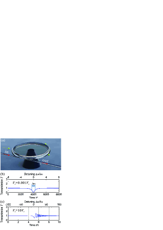
Figure 1: (Color online) (a) Schematic illustration of microcavity sensor for nanoparticle detection. A silica microtoroid is coupling with a silica fiber taper, with laser being loaded from one port and transmitted light being collected from the other. (b) Typical quasi-static transmission spectrum of whispering gallery mode, with the laser frequency sweeping speed $V_{s}=0.001V_{c}$ where the character sweeping speed is $V_{c}=4\kappa^{2}$. (c) A transient transmission spectrum for fast scanning laser, with $V_{s}=10V_{c}$. Time normalized with $\tau=\frac{1}{\kappa}$.

Figure 1(a) shows a typical microcavity sensor composed of a toroid microcavity and a tapered fiber 09NP ; 11PNAS . A probe light is guided in the single mode tapered fiber, and coupled with the high-Q whispering gallery modes (WGMs) in the microcavity through evanescent field. When there is variation of the environment, such as the nanoparticle approaching or leaving the microcavity, the intrinsic loss and resonant frequency of the WGMs will be disturbed. Then, the phase and amplitude of the cavity field will change accordingly.

The electric field component of input light generally reads $s_{in}(t)=S_{in}e^{-j\phi(t)}$, where $j$ is the square root of $-1$. The phase $\phi(t)$ is the integral of instant angular frequency $\omega(t)$ about time $t$, i.e., $\phi(t)=\int\omega(t)dt$ . The amplitude $a(t)$ of WGM field can be solved by the coupled mode theory book ; 08JOSAB ; 99JOSAB

$$\frac{da(t)}{dt}=-j\omega_{i}a(t)-(\kappa_{i}+\kappa_{e})a(t)+\sqrt{2\kappa_{e}}s_{in}(t).$$ (1)

Here, $\omega_{i}$ and $\kappa_{i}$ are the angular frequency and intrinsic loss rate of photons, which are determined by the material and the geometry of the microcavity. The $\kappa_{e}$ is external loss of photons cause by the fiber taper, which can be controlled by adjusting the relative location of fiber taper in respect to the microcavity. Denote the total decay rate of the field amplitude as $\kappa=\kappa_{i}+\kappa_{e}$, and hence the total quality factor $Q=\omega_{i}/2\kappa$. Moreover, the total amplitude lifetime of photons in the mode is $\tau=1/\kappa$.

In experiments, the laser amplitude is fixed to reduce the noises induced by amplitude fluctuation in sensor application, thus $S_{in}$ is a constant. For monochrome light with fixed laser frequency, $\phi(t)$ increases with time $t$ linearly, i.e. $\phi(t)=\omega_{in}t$ , we obtain the steady state solution as

$$a(t)=\frac{\sqrt{2\kappa_{e}}S_{in}e^{-j\omega_{in}t}}{j(\omega_{in}-\omega_{i})+(\kappa_{i}+\kappa_{e})}.$$ (2)

The cavity field approaches the steady state with the build-up time in the order of $\tau$. For the WGM, there is another time scale $\tau_{c}$, which is the round trip time corresponding to the period that a pulse travels around the perimeter of a microcavity. In high $Q$ microcavity, the $\tau\gg\tau_{c}$ is satisfied, which implies that photons travel thousands of times in the microcavity before they lost. The high sensitivity of microcavity sensor benefits from this repeated travels. Furthermore, we assume the time scales of all interactions is much longer than the $\tau_{c}$, so the Eq. (1) is always true.

In practice, the transmission spectrum are obtained by sweeping the frequency of the probe laser. For example, a linear frequency scanning $\omega(t)=\omega_{in}+V_{s}t$ (in the following, the scanning speeds is defined in terms of the angular frequency) is usually employed, then

$$\phi(t)=\int_{0}^{t}\omega(t^{\prime})dt^{\prime}=\omega_{in}t+\frac{V_{s}}{2}t^{2}.$$ (3)

A general solution of Eq. (1) reads

$$a(t)= \sqrt{2\kappa_{e}}S_{in}e^{j\omega_{i}t-\kappa t}\left[\frac{\tau}{1+j(\omega_{in}-\omega_{i})\tau}\right.$$

$$\left.+\int_{0}^{t}e^{j\phi(t^{\prime})-j\omega_{i}t^{\prime}+\kappa t^{\prime}}dt^{\prime}\right].$$ (4)

So long as we know the function $\phi(t)$, the cavity field $a(t)$ can be solved accurately by Eq. (4). For the linear scanning case [Eq. (3)], the equation can be solved analytically 14SR . For more general cases with nonlinear scanning, $a(t)$ should be solved numerically.

The transmission signal

$$s_{out}(t)=s_{in}(t)-\sqrt{2\kappa_{e}}a(t)$$ (5)

corresponding to the interference of the directly-transmitted input laser and cavity output in the tapered fiber. The intensity of transmitted signal ($|s_{out}(t)|^{2}$) is collected and monitored by a high-speed photon detector in real-time. For convenience, people measure the intensity spectrum of output signal normalized by input signal

$$T(t)=|s_{out}(t)/s_{in}(t)|^{2}$$ (6)

to gather information from spectrum of intensity, but the phase information cannot be obtained without interferometer which requires complex stabilization equipments.

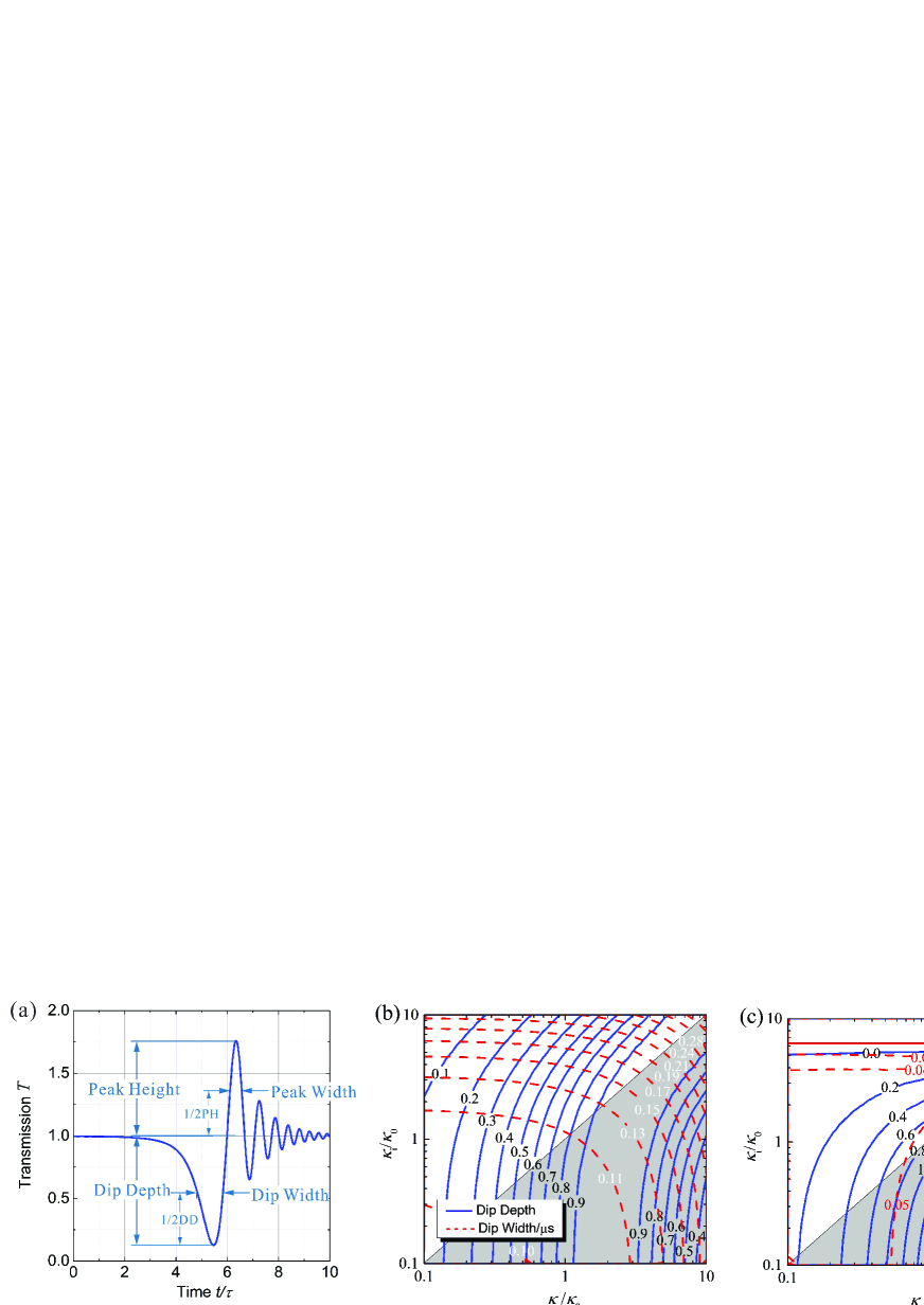
Figure 2: (Color online) (a) Typical transmission against time of transient sensor at critical coupling, for $\kappa_{i}=\kappa_{e}=\kappa_{0}$ with $\kappa_{0}=3.0\>\mathrm{MHz}$. (b) and (c) are diagrams for checking coupling parameters by the values of dip width and depth or the peak width and height. The vertical coordinate is $\kappa_{i}/\kappa_{0}$, and the abscissa is $\kappa_{e}/\kappa_{0}$ in logarithm scale with $\kappa_{0}$. The diagonal dash line denotes critical coupling condition for steady state. Areas under (shade triangle) and upper the diagonal line correspond to over- and under- coupling regimes, respectively.

Here, we introduce the character speed $V_{c}=4/\tau^{2}=4(\kappa_{i}+\kappa_{e})^{2}$, which corresponds to the speed that the laser sweep through the cavity resonance (frequency range $2/\tau$) within the lifetime of the mode $(2\tau)$. When the scanning speed $V_{s}=0.001V_{c}\ll V_{c}$, the transmission shows the typical symmetry Lorentz spectrum, as shown in Fig. 1(b) for critical coupling where $\kappa_{i}=\kappa_{e}$. In this case, the transient response of the WGM can be neglected and the field amplitude can be approximated by the steady state solution (Eq. (2)). However, in Eq. (6) the information about the phase of the transmitted light is lost, and we cannot distinguish between the under- and over-coupling since the roles of $\kappa_{i}$ and $\kappa_{e}$ in Eq. (2) are identical. Then, we cannot distinguish the change of the intrinsic cavity loss due to the sensing event from the change of the external cavity loss due to vibration of tapered fiber.

For fast sweeping speed that $V_{s}$ is comparable with or even larger than $V_{c}$, the transient response of the cavity field cannot be omitted. For instance, the spectrum of $V_{s}=10V_{c}$ is shown in Fig. 1(c), where other parameters are the same with Fig. 1(b). As firstly pointed out in Ref. 08JOSABYDumeige , the information of $\kappa_{i}$ and $\kappa_{e}$ can be extracted from the transient response deterministically. It can be understood intuitively that the coupled microcavity and fiber taper system becomes a heterodyne interferometer for transient sensor. Due to the high-Q WGM, there is a hysteresis between the input light and cavity output light, or we can say the light emitted from the cavity is actually the light input from the fiber a while ago. When $V_{s}$ is large, the detected light is the interference between lights of different frequencies, thus it contains both the amplitude and phase information of the cavity field.

III Transient Response of Microcavity

In general, there are two ways to monitor the variation of cavity resonance. One is sweeping the laser frequency quickly and repeatedly. The frequency $\omega(t)$ is a linear function with time, then the phase $\phi(t)$ is a quadratic function of time. Since each frequency sweeping takes a repetition time $P$, we can refresh the information of environment at digital time $nP$ ($n$ is an integer). The other approach is locking the laser frequency precisely, and then monitoring the change of transmitted signal due to the change of resonant frequency. In the later case, the relevant $\phi(t)=\int\omega(t)dt$ is very complicated, which is determined by the history of the variation of environment. For both cases, the principle and applied theory are the same with those described in previous section.

III.1 Sweep Laser Frequency

The resonant frequency of a cavity can be characterized by monitoring the position of dip in transmission spectrum of steady state in experience. In addition, relying on the transient response analysis, people has figured out how to get $\kappa_{e}$ and $\kappa_{i}$ from the parameter fitting method 08JOSABYDumeige ; 09COL . Here, we provide a direct way to determine the coupling rates by the features of transmission curves $T(t)$ in transient states. To show the results quantitatively, we choose the following parameters which are reasonable in experiments: resonant wavelength $\lambda_{i}=1.55\ \mu\mathrm{m}$ and $Q_{i}=2\times 10^{8}$. The critical sweep speed for such high-Q cavity with critical coupling is $V_{c}=4(\frac{\omega_{i}}{Q_{i}})^{2}\approx 148\ \mathrm{MHz}/\mu\mathrm{s}$. When the frequency of the input signal scans fast (e.g. $V_{s}=100\mathrm{MHz}/\mu\mathrm{s}\approx 0.67V_{c}$) through a resonant frequency of the microcavity, an asymmetry dip followed with a ringing tail is the typical shape of $T(t)$ (Fig. 2(a)), in contrast to a simple symmetry Lorenz lineshape dip of $T(t)$ in steady state assumption. Because of the transient process that light builds up inside the cavity, the dip bottom in on-resonance moment does not reach $0$. The ringing tail is the result of interference between back coupled WGM light and the transmitted signal light. Besides, for a system being free from nonlinear effect 09COL , if the input signal scans downward ($-V_{s}$) through the resonant frequency, the transmission curve is the same in time sequence as it scans upward.

The analytical solution of the integral in Eq. (4) can be written as 14SR

$$a(t)=\sqrt{2\kappa_{e}}S_{in}e^{j\omega_{i}t-\kappa t}\left[f(t)-f(0)+\frac{1}{\kappa+j(\omega_{in}-\omega_{i})}\right],$$ (7)

where

$$f(t)=-\sqrt{\frac{j\pi}{2V_{s}}}e^{-\frac{[j(\omega_{in}-\omega_{i})+\kappa]^{2}}{2V_{s}}}\mathrm{erf}(\frac{j\kappa+\omega_{i}-\omega_{in}-V_{s}t}{\sqrt{2jV_{s}}})$$ (8)

and $\mathrm{erf}(z)$ is the complex error function.

The transmission curve can be characterized by four parameters: peak height, peak width, dip depth and dip width [Fig. 2(a)], where peak width is the full width of half maximum of the first peak, dip width is the full width of half minimum of the first dip. Varying $\kappa_{i}$ and $\kappa_{e}$ and fixing $V_{s}=2V_{0}\approx 296\ \mathrm{MHz}/\mu\mathrm{s}$, these parameters are extracted, and are plotted in Figs. 2(b) and (c). Noting that the absolute position of the dip is not shown here, which corresponding to the shift of cavity resonance, because it can be determined in experiment precisely with the help of another reference cavity.

If both the $\kappa_{i}$ and $\kappa_{e}$ are large enough to make $V_{s}\ll V_{c}=4(\kappa_{i}+\kappa_{e})^{2}$ (top right of Fig. 2(b)), it is the quasi-steady state where the dip depth depends on the ratio $\kappa_{i}/\kappa_{e}$. When $\kappa_{i}\approx\kappa_{e}$, the dip depth is around $1$ corresponding to the critical coupling. However, when decreasing the $\kappa_{i}$ and the $\kappa_{e}$, the critical coupling deviates from the line $\kappa_{i}=\kappa_{e}$. When $\kappa_{i}$ is small (lower half of Fig. 2(b)) the dip depth mainly depends on $\kappa_{e}$ , and the extreme value of dip depth appears near the $\kappa_{e}\approx 2\kappa_{0}$. It is because that when $V_{s}>V_{c}$, the critical coupling for transient response requires $\kappa_{e}>\kappa_{i}$ to make energy enter the cavity more efficiently and afterwards destructively interference with the input light, leads to a cancelation of transmission. However, if the $\kappa_{e}$ is too large, the energy of cavity couples back to tapered fiber faster, thus break the balance and give non-zero transmission. So, as analogue to the steady state critical coupling, the certain $\kappa_{e}$ give rise to temporal critical coupling that dip depth be unitary.

In both Figs. 2(b) and (c), in the transient region that $V_{s}\geq V_{c}$, the contours of the width and height of peak and the width and depth of dip cross, respectively. Therefore, the transient transmission provides extra information from which we can determine the value of $\kappa_{i}$ and $\kappa_{e}$. For example, if a coupling system has a transmission curve with a dip depth of $0.8$ and dip width of $0.13$, it may in over or under coupling region (see Fig. 2(b)). Then check the peak width, assume $0.07\ \mu\mathrm{s}$ to obtain the value of $\kappa_{i}\approx 3.2\kappa_{0}$ and $\kappa_{e}\approx 4.4\kappa_{0}$. There even exists other redundant feature (peak height) to double check the result. Therefore, combining with the measured location of the resonance, we can estimate the instant frequency and decay rate of the WGM for sensing purpose.

More generally, for any given $V_{s}$, we can normalize the transmission $T(t)$ (Eqs. (7) and (8)) by replacing $\kappa/\sqrt{V_{s}}$ with $\kappa^{\prime}$ and $t\sqrt{V_{s}}$ with $t^{\prime}$, respectively. Then the $\kappa_{i}$, $\kappa_{e}$, and $\omega_{i(in)}$ are rescaled with a factor of $1/\sqrt{V_{s}}$, and replaced with corresponding prime variables too. After the transformation, $T$ is independent of $V_{s}$, so the charts of Figs. 2 (b) and (c) are sufficient to estimate the $\kappa_{i}$ and $\kappa_{e}$ at any really applied sweep speed $V_{s}$. For example, if the sweep speed is $V_{s}=8V_{0}$, the measured peak/dip width should be rescaled with a factor of $2$. Using the rescaled widths to find out the apparent $\kappa_{i(e)}$ from the Figs. 2(b) and (c), and rescale back the result $\kappa_{i(e)}$ with a factor of $2$ to get the real $\kappa_{i(e)}$ at current sweep speed.

III.2 Fixed Laser Frequency

For the other method, a coupled microcavity and tapered fiber system can be calibrated and stabilized with fixed coupling and loss rates, and the frequency of the incident probe light is locked to the cavity resonance. The environment variation will change the dielectric properties of the cavity and cause a change of $\omega_{i}$, then the detuning $\Delta\omega$ between probe light and cavity mode $\omega-\omega_{i}$ occurs, resulting in the change of transmittance. It has been proved in Fabry-Perot cavity that the linear increase of $\omega_{i}$ is equivalent to the decrease of $\omega$ with similar scanning speed 02AO . Therefore, a persistent changing of $\omega_{i}$ at relatively high speed can generate a transient ringing transmission line too.

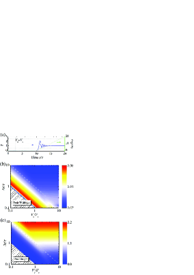
Figure 3: (a) The transmission response based on linear variation of resonance frequency beginning with critical coupling. The peak width (b) and height (c) varied with resonance sweeping speed and elapse time.

Taking a linear change of $\omega_{i}$ 11APL and initial critical coupling as an example, we investigate the feature of the transient transmission. For a general consideration, we study the spectrum for various cavity frequency change frequency and dynamic range, thus solve the temporal transmission numerically. A typical transmission curve is shown in Fig. 3(a). In this example, the change of $\omega_{i}$ begin at time $10\tau$. The transmittance is zero when $t<10\tau$ because the system state is kept in critical coupling and the probe light is absorbed by the cavity completely. When $\omega_{i}$ start to change due to environment perturbation, the balance between the input laser and cavity leakage is broken suddenly, then a ringing line shape is formed. This scenario is similar as the case studied in previous subsection, where the laser frequency is sweeping while the cavity frequency is fixed. But, when the sweep speeds are the same the peak height is higher now than that in the sweep laser case.

In practice, $\omega_{i}$ may drifts in a period of time $\Delta t$ at sweep speed $V_{s}$, then reaches the equilibrium position with the final detuning $\Delta\omega=V_{s}\Delta t$. Then, the ringing tail will end to the steady state transmission level $T_{s}=(\triangle\omega)^{2}/(1/\tau^{2}+(\triangle\omega)^{2})$, which may less than unit evidently. Correspondingly the definitions of peak height and peak width of $T(t)$ are modified according to the horizon line of $T=T_{s}$, as compare to Fig. 2(a). Peak width and peak height vary with $\Delta t$ and $V_{s}$ (Figs. 3 (b) and (c)). In those figures of double logarithmic coordinates, $\Delta\omega$ on each of lines paralleling the diagonal dash line, on which $\Delta\omega$ equals two times of line-width, are constant. In the lower left of the figures, shaded triangle infers there is no peak higher than $T_{s}$. However, in this regime, the total frequency change is still within the cavity resonance and the change of cavity resonance is slow, the environment change can be estimated through quasi-static cavity response. At the right vertex of the triangle, though the sweep speed is as fast as critical speed, the short elapse time $0.1\tau$ makes a narrow detuning $\Delta\omega\approx 0.2\times(2/\tau)$. It means the $T_{s}\approx 0.14$, and in the time of sweeps, transmission is kept at the relative flat bottom of Lorentz line-shape. The relative gentle variation of the transmission restrains the ringing phenomena. When the $\Delta\omega$ gets larger, first a broaden low peak arises, then it becomes sharper and higher.

Furthermore, if the $\Delta\omega$ is larger than two times of line-width (right upper region of the figures), the peaks are no longer varied with $V_{s}$, especially in high speed side. This saturation about speed can be understood as the response time of the microcavity is limited to life time $2\tau$. Though the $\omega_{i}$ drifts beyond the resonant frequency in a short time far less that $2\tau$ at high sweep speed, the energy in the microcavity leaks out the cavity with its own pace. In addition, comparing the saturated peak height on the most right vertical line with the color bar, we can find peak height is proportional to $\log\Delta t$.

III.3 Comparison

For the two different approaches, we can find there are many differences. In the sweeping laser case, the frequency range of the sweeping is usually in the order of $2\pi\times 10\sim 100$ GHz, which provide a wide dynamic range of the sensor. However, for a fixed sweeping speed $V_{s}$, the larger dynamic range also means longer repetition time $P$ for the laser sweeping through the wide frequency range. For example, the frequency of WGM in the silica microcavity may change by $2\pi\times 1.7$ GHz when the environment temperature changes by $1\ \mathrm{K}$ 11OE . If the sweeping speed $V_{s}=2\pi\times 200\ \mathrm{MHz}/\mu\mathrm{s}$ and frequency range is $2\pi\times 200$ GHz, the dynamic range of the temperature sensor is $117$ K while $P=1\ \mathrm{ms}$. If the frequency range reduced by $100$ times, the dynamic range will only be $1.17$ K while $P=10\ \mu\mathrm{s}$. Therefore, there is a trade-off between the temporal resolution and dynamic range. Note that the sweeping laser transient sensor pre-assumed that the environment induced change speed of frequency or decay rate is much slower than $V_{s}$. For a given $V_{s}$, higher Q gives higher sensitivity.

In contrast, the fixed frequency case show a much smaller dynamic range, which can only sense the event with frequency shift smaller than the linewidth, and is usually several orders of magnitude smaller than that in the sweeping laser case. The benefit is that this type of transient sensors can response to the external perturbation quickly within the time-window of $1\sim 100\,\mathrm{ns}$, which is $4-6$ orders smaller than $P=1\ \mathrm{ms}$ in the sweeping laser case. For example, a nanoparticle pass through the cavity may induce a small frequency change within $1\ \mu\mathrm{s}$. This event may be missed for the sweeping laser case, but can be monitored by the fixed laser case. There is a trade-off between the dynamic range (linewidth of resonance) and response time (lifetime of resonance), and the sensitivity is also related to the linewidth.

Therefore, the two different transient sensors are appropriate for different applications. When the perturbation induced frequency shift is very large but relatively slow, we can use the sweeping laser. When the perturbation is small but very fast, we can use the fixed laser. In both cases, an external reference cavity is required, which is used as frequency reference in the laser sweeping case or to lock the laser frequency for the fixed laser frequency case.

It’s also worth to note that the sensitivity of the transient sensor can also be improved comparing with that in the slowly sweeping case. In the transient response, the ringing transmission curve is sharper due to increased slope of $dT/d\omega$ (the time is usually converted to frequency by $V_{s}$ in experiment). For example, the maximum slope (the first ring up) for $V_{s}=2V_{c}$ is about 4 times larger than the maximum slope for $V_{s}\ll V_{c}$. In addition, the refresh rate is also increased by increasing $V_{s}$. One may argue that the shot noise of the laser also increase for faster sweeping laser, since the duration of time to sweep through the cavity resonance is proportional to $1/V_{s}$. This can be improved by increasing the laser power for sweeping, the only limitation is that the power absorbed by the cavity should be smaller to avoid thermal or Kerr effect. Similarly, the slope will be larger for faster perturbation in the fixed laser frequency case, where the sensitivity depends on sensing event but not the equipments in experiments.

IV Example: Transient Nanoparticle Sensor

In this section, we will analyze the practical application of the microcavity sensor for transient nanoparticle motion. The nanoparticle sensor can be used for study the kinetic properties of the nanosized particles, with micrometer-scale spatial resolution, and microsecond-scale temporal resolution. Use the setup demonstrated recently 11NN , we can explore the mechanics, fluid dynamics and stochastic Brownian motion with unprecedented precision. When a nanoparticle approaches the microcavity, it shifts the resonance ($\omega_{i}$), and also increases the loss of the microcavity by scattering. But in high $Q$ microcavity, the internal lifetime $\tau_{i}$ mainly depends on the absorption loss of the cavity material. Scattering loss like binding a nanoparticle or carving a small notch does not affect the lifetime much 10PNAS . So we can safely ignore the change of the $\tau_{i}$, and fix the system in critical coupling region. In the following, we study the transient sensor initialized in critical coupling region, when the particles are far away.

IV.1 Binding

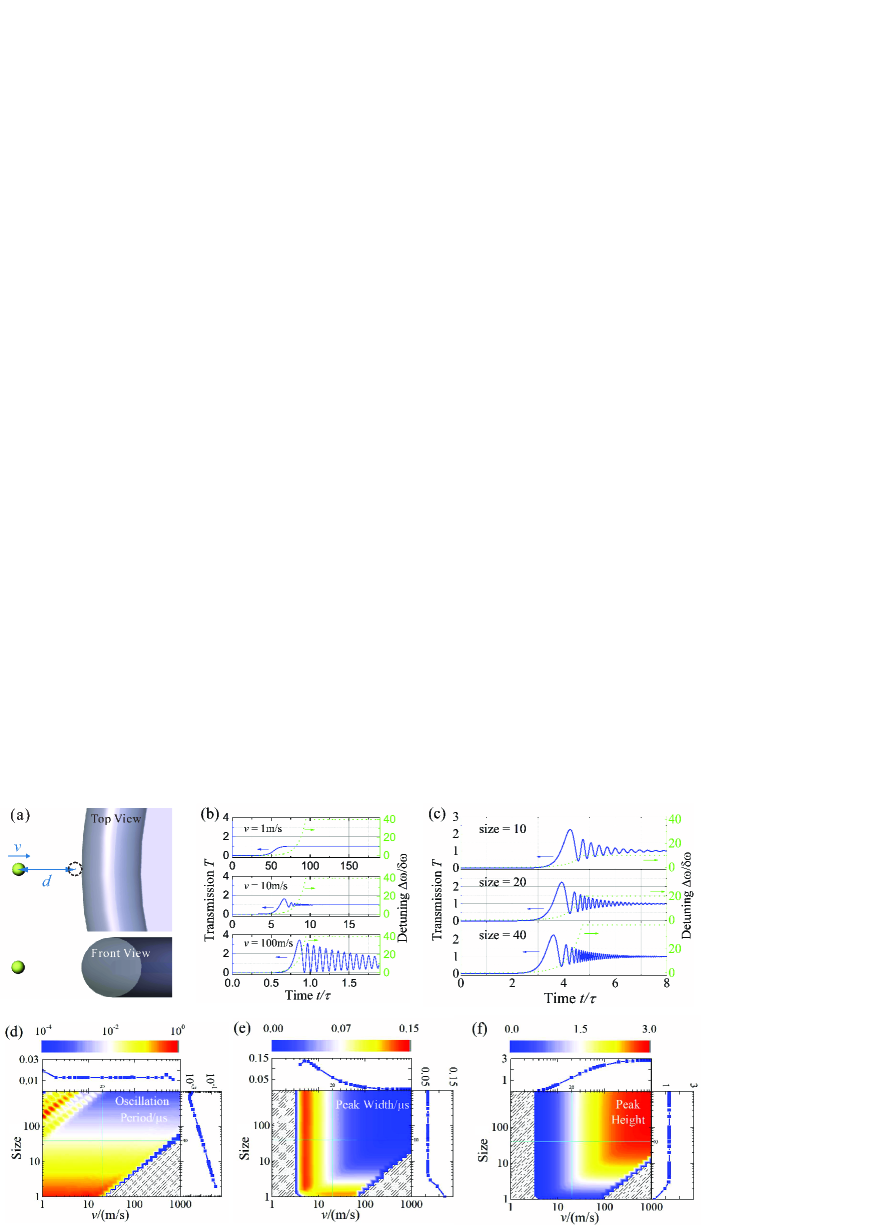
Figure 4: (a) Schematic illustration of the binding nanoparticle sensing, where a particle approaches to the side of cavity and then adhere on it; (b) and (c) the transmissions $T(t)$ for fixed probe laser frequency for different particle traveling speed ($v$) and sizes ($\epsilon$). (d)-(f) The features of the transmission versus $v$ and $\epsilon$.

As illustrated in Fig. 4(a), a nanoparticle approaches the microcavity along a trace perpendicular to the outer rim, then is bound Su2015Label on the surface . The nanoparticle shifts the frequency of a mode by moving into the evanescent field of the mode. The degree of the shift is proportional to local field intensity 03OL . Besides, the evanescent field of a mode decays (decay factor $\alpha$) exponentially along with the distance $d$. Therefore, a nanoparticle approaching the microcavity with constant velocity $v$ will induce a mode frequency shift which is exponentially increase with time (Figs. 4(b) and (c) the first half of dotted green line)

$$\omega(t)=\omega_{i}(1-\epsilon e^{-\alpha(d_{0}-vt)}).$$ (9)

Here for the convenience of symbol system, the variation of $\omega_{i}$ has been equivalently transferred to $\omega(t)$. At time $t=0$, the nanoparticle is in distant $d_{0}$ ($\alpha d_{0}\gg 1$), and $\omega(0)\approx\omega_{i}$. When the nanoparticle touches the microcavity and be adhered to it, the $\omega(t)=\omega(d_{0}/v)$ for $t>d_{0}/v$ is a constant (the last half of dotted green line in Figs. 4(b) and (c)). The $\epsilon$, depending on inherent electromagnetic attributes of the particle, represents the degree of frequency shifting when the particle is bound on the surface. Replace the $\omega(t)$ of Eq. (4) with the Eq. (9), we can get the transmission $T(t)$ numerically.

Set $\epsilon=size/Q=40/Q$, which means the maximum shift $\epsilon\omega_{i}$ is $40$ times of linewidth. Other parameters are the same with that in Section III. Firstly, the transmission and its features varying with speed of the particles are investigated. The transmissions $T(t)$ of various speeds are shown in Fig. 4(b). Similar to the previous analysis, the transient frequency shift induces ringing phenomena, the peak value increases with the increasing of speeds. In addition, the transmission for different particle sizes/volumes are studied, as shown in Fig. 4(c). Since the total resonant frequency shift $\epsilon$ is proportional to size/volume of the particle, the effective frequency shifting speed increases with the size. According to equations (6) in Ref. 88OL , the oscillation period of ringtail is inversely correlated to $\epsilon$ and thus decreases with increasing of size.

The basic features, including oscillation period, peak width and peak height, varying with the particle size and speed are plotted in Figs. 4(d)-(f). Using the features measured in experiments, we can identify the particle size and speed, since they correlate with these parameters in quite different ways. For example, from the curves extracted from the 2D maps, when size=40, the oscillation period is almost constant (Fig. 4(d) up panel), while peak width (Fig. 4(e) up panel) and height (Fig. 4(f) up panel) vary; when speed is fixed by 20 m/s, the period almost inversely proportional to size (Fig. 4(d) right panel), while the other two features remains the same (Figs. 4(e) and (f) right panels). Although the regime for small $v$ does not show ringing phenomena, but it’s quasi-static process, we can determine the size and velocity from the slowly varing transmission line. For the down-right coner in Figs. 4(e) and (f), there is also no ringing because the transient sensor is ultimately limited by the cavity lifetime.

IV.2 Passing-by

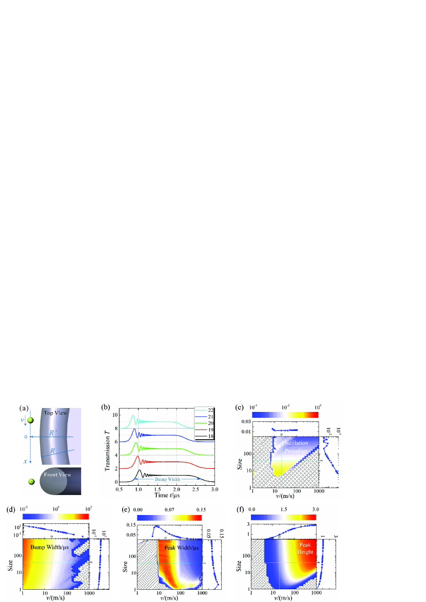
Figure 5: (a) Schematic illustration of the passing-by nanoparticle sensing . The radius of microcavity is $R$, the aim distance is $R^{\prime}$. (b) The transmission $T(t)$ varies with speed. Curves are shifted up for clear show. (c)-(f) are the features: oscillation period, bump width, peak width, and peak height versus nanoparticle size and speed.

In another practical sensor scenario, nanoparticle passes by the microcavity in a tangential way (Fig. 5(a)). Set $x$ axis along the path. Its positive direction is the direction of velocity of the nanoparticle. Original point $x=0$ is the point which is nearest to the microcavity on the path. Then, the frequency shift reads

$$\omega(t)=\omega_{i}(1-\epsilon e^{-\alpha(\sqrt{R^{\prime 2}+(x_{0}+vt)^{2}}-R)}).$$ (10)

The $x_{0}(<0)$ is the initial position of nanoparticle when $t=0$. The nanoparticle stays in the effective couple range in a short time inversely proportional to speed (Fig. 5(b)). In the $T(t)$ curve, we define bump width with full-width at $T=0.5$ to character it (Fig. 5(b) button panel). The characters of the $T(t)$ concerning different particle speeds and sizes are performed (Figs. 5(c)-(f)). Like the binding case, the period is only related to the size. The peak height, peak width and the bump width mainly vary with the speed.

At first glance, the contours of features of $T(t)$ in the case of passing by are like that in the case of binding, except for a new feature bump width. But in detail investigation, the variations of features depicted in Fig. 5 are complicated than their counterpart in Fig. 4. Because in content of frequency shift, Eq. (10) is more complicated than the simple exponential relationship depicted by Eq. (9). The Eq. (10) is a exponential function, when $|x_{0}+vt|\gg R^{\prime}$ (i.e., particle is far away from the microcavity). While it is simplified to a Gaussian function, when $|x_{0}+vt|\ll R^{\prime}$. Then the actual frequency shift is between the two extreme situations. Based on the Figs. 4 and 5, we find that the oscillation period is suitable to characterize the particle size in experiment. The peak width has the best sensitivity to detect particle speed when particle size is not less than 5.

V Conclusions

In summary, based on the transient transmittance of high-Q microcavities, the environment variation can be sensed with both high sensitivity and high temporal resolution. In addition to the enhanced frequency shift sensing, we can also sense the intrinsic and external cavity loss. Especially, we studied the motive nanoparticle sensing and demonstrated that the speed and size of a nanoparticle can be determined by the experiment-measurable transmission. We believe that our studies opens a door to fast dynamic sensing by microcavity. Combining with the package technique, we would expect to bring the fiber integrated optical microcavity sensors 11OE ; Wang2012 ; Pevec2011 out of lab for ultrafast and ultrasensitive detections.

Note added: During the preparation of this manuscript, a related experiment work published Rosenblum2015 , where a cavity ring-up spectroscopy with submicrosecond time resolution by abruptly turn-on a far-detuned probe laser pulse is demonstrated.

Funding Information

“Strategic Priority Research Program(B)” of the Chinese Academy of Sciences (XDB01030200); National Basic Research Program of China (2011CB921200, 2011CBA00200); National Natural Science Foundation of China (NSFC) (11204169); the Young Core Instructor Foundation from the Education Department of Henan Province, China (2013GGJS-163); Open Project of Key Laboratory of Quantum Information (KQI201502); Army Research Office (ARO) (W911NF-12-1-0026).

References

- (1) F. Vollmer and L. Yang, “Review label-free detection with high-Q microcavities: a review of biosensing mechanisms for integrated devices,” Nanophotonics 1, 267–291 (2012).
- (2) J.-R. Carrier, M. Boissinot, and C. Nì. Allen, “Dielectric resonating microspheres for biosensing: An optical approach to a biological problem,” Am. J. Phys. 82, 510–520 (2014).
- (3) Y. Yang, J. Ward, and S. N. Chormaic, “Quasi-droplet microbubbles for high resolution sensing applications,” Opt. Express 22, 6881–6898 (2014).
- (4) Ş. K. Öezdemir, J. Zhu, X. Yang, B. Peng, H. Yilmaz, L. He, F. Monifi, S. H. Huang, G. L. Long, and L. Yang, “Highly sensitive detection of nanoparticles with a self-referenced and self-heterodyned whispering-gallery Raman microlaser,” P. Natl. Acad. Sci. USA 111, E3836–E3844 (2014).
- (5) B.-B. Li, W. R. Clements, X.-C. Yu, K. Shi, Q. Gong, and Y.-F. Xiao, “Single nanoparticle detection using split-mode microcavity Raman lasers,” P. Natl. Acad. Sci. USA 111, 14657–14662 (2014).
- (6) F. Sedlmeir, R. Zeltner, G. Leuchs, and H. G. L. Schwefel, “High-Q MgF2 whispering gallery mode resonators for refractometric sensing in aqueous environment,” Opt. Express 22, 30934–30942 (2014).
- (7) J. M. Ward, N. Dhasmana, and S. N. Chormaic, “Hollow core, whispering gallery resonator sensors,” Eur. Phys. J.-Spec. Top. 223, 1917–1935 (2014).
- (8) M. R. Foreman, J. D. Swaim, and F. Vollmer, “Whispering gallery mode sensors,” Adv. Opt. Photonics 7, 168–240 (2015).
- (9) J. Su, “Label-free single exosome detection using frequency-locked microtoroid optical resonators,” ACS Photonics 2, 1241–1245 (2015).
- (10) I. A. Grimaldi, G. Testa, and R. Bernini, “Flow through ring resonator sensing platform,” RSC Advances 5, 70156–70162 (2015).
- (11) S. L. McCall, A. F. J. Levi, R. E. Slusher, S. J. Pearton, and R. A. Logan, “Whispering-gallery mode microdisk lasers,” Appl. Phys. Lett. 60, 289–291 (1992).
- (12) M. C. Collodo, F. Sedlmeir, B. Sprenger, S. Svitlov, L. J. Wang, and H. G. L. Schwefel, “Sub-kHz lasing of a CaF2 whispering gallery mode resonator stabilized fiber ring laser,” Opt. Express 22 (2014).
- (13) P. DelHaye, A. Schliesser, O. Arcizet, T. Wilken, R. Holzwarth, and T. Kippenberg, “Optical frequency comb generation from a monolithic microresonator,” Nature 450, 1214–1217 (2007).
- (14) T. J. Kippenberg, R. Holzwarth, and S. A. Diddams, “Microresonator-based optical frequency combs.” Science 332, 555–9 (2011).
- (15) T. J. Kippenberg and K. J. Vahala, “Cavity optomechanics: back-action at the mesoscale,” Science 321, 1172–1176 (2008).
- (16) C. Dong, V. Fiore, M. C. Kuzyk, and H. Wang, “Optomechanical Dark Mode,” Science 338, 1609–1613 (2012).
- (17) R. Madugani, Y. Yang, J. M. Ward, V. H. Le, and S. N. Chormaic, “Optomechanical transduction and characterization of a silica microsphere pendulum via evanescent light,” Appl. Phys. Lett. 106 (2015).
- (18) T. Aoki, B. Dayan, E. Wilcut, W. P. Bowen, a. S. Parkins, T. J. Kippenberg, K. J. Vahala, and H. J. Kimble, “Observation of strong coupling between one atom and a monolithic microresonator.” Nature 443, 671–4 (2006).
- (19) I. Shomroni, S. Rosenblum, Y. Lovsky, O. Bechler, G. Guendelman, and B. Dayan, “All-optical routing of single photons by a one-atom switch controlled by a single photon,” Science 453, 1023–30 (2014).
- (20) N. Hanumegowda, C. Stica, B. Patel, I. White, and X. Fan, “Refractometric sensors based on microsphere resonators,” Appl. Phys. Lett. 87 (2005).
- (21) R. Zeltner, F. Sedlmeir, G. Leuchs, and H. G. L. Schwefel, “Crystalline MgF2 whispering gallery mode resonators for enhanced bulk index sensitivity,” Eur. Phys. J.-Spec. Top. 223, 1989–1994 (2014).
- (22) F. Vollmer, S. Arnold, and D. Keng, “Single virus detection from the reactive shift of a whispering-gallery mode,” P. Natl. Acad. Sci. USA 105, 20701–4 (2008).
- (23) L. He, Ş. K. Özdemir, J. Zhu, W. Kim, and L. Yang, “Detecting single viruses and nanoparticles using whispering gallery microlasers,” Nat. Nanotechnol. 6, 428–432 (2011).
- (24) T. Lu, H. Lee, T. Chen, S. Herchak, J.-H. Kim, S. E. Fraser, R. C. Flagan, and K. Vahala, “High sensitivity nanoparticle detection using optical microcavities,” P. Natl. Acad. Sci. USA 108, 5976–5979 (2011).
- (25) Y.-Z. Yan, C.-L. Zou, S.-B. Yan, F.-W. Sun, Z. Ji, J. Liu, Y.-G. Zhang, L. Wang, C.-Y. Xue, W.-D. Zhang, Z.-F. Han, and J.-J. Xiong, “Packaged silica microsphere-taper coupling system for robust thermal sensing application,” Opt. Express 19, 5753–5759 (2011).
- (26) P. Wang, M. Ding, G. S. Murugan, L. Bo, C. Guan, Y. Semenova, Q. Wu, G. Farrell, and G. Brambilla, “Packaged, high-Q, microsphere-resonator-based add–drop filter,” Opt. lett. 39, 5208–5211 (2014).
- (27) T. Ioppolo and M. V. Oetuegen, “Pressure tuning of whispering gallery mode resonators,” J. Opt. Soc. Am. 24, 2721–2726 (2007).
- (28) R. Madugani, Y. Yang, J. M. Ward, J. D. Riordan, S. Coppola, V. Vespini, S. Grilli, A. Finizio, P. Ferraro, and S. N. Chormaic, “Terahertz tuning of whispering gallery modes in a PDMS stand-alone, stretchable microsphere,” Opt. Lett. 37, 4762–4764 (2012).
- (29) L. Stern, I. Goykhman, B. Desiatov, and U. Levy, “Frequency locked micro disk resonator for real time and precise monitoring of refractive index,” Opt. Lett. 37, 1313–1315 (2012).
- (30) T. Carmon, L. Yang, and K. Vahala, “Dynamical thermal behavior and thermal self-stability of microcavities,” Opt. Express 12, 4742–4750 (2004).
- (31) S. Soltani and A. M. Armani, “Optothermal transport behavior in whispering gallery mode optical cavities,” Appl. Phys. Lett. 105, 051111 (2014).
- (32) C. Dong, C. Zou, J. Cui, Y. Yang, Z. Han, and G. Guo, “Ringing phenomenon in silica microspheres,” Chin. Opt. Lett. 7, 299–301 (2009).
- (33) A. Rasoloniaina, V. Huet, T. K. Nguyen, E. Le Cren, M. Mortier, L. Michely, Y. Dumeige, and P. Feron, “Controling the coupling properties of active ultrahigh-Q WGM microcavities from undercoupling to selective amplification,” Sci. Rep. 4, 4023 (2014).
- (34) B. Wang, T. Siahaan, M. A. Dündar, R. Nötzel, M. J. van der Hoek, S. He, and R. W. van der Heijden, “Photonic crystal cavity on optical fiber facet for refractive index sensing.” Opt. Lett. 37, 833–835 (2012).
- (35) S. Pevec and D. Donlagic, “All-fiber, long-active-length Fabry-Perot strain sensor.” Opt. Express 19, 15641–51 (2011).
- (36) J. Zhu, Ş. K. Özdemir, Y.-F. Xiao, L. Li, L. He, D.-R. Chen, and L. Yang, “On-chip single nanoparticle detection and sizing by mode splitting in an ultrahigh-Q microresonator,” Nat. Photonics 4, 46–49 (2009).
- (37) H. A. Haus, Waves and fields in optoelectronics, vol. 464 (Prentice-Hall Englewood Cliffs, NJ, 1984).
- (38) C.-L. Zou, Y. Yang, C.-H. Dong, Y.-F. Xiao, X.-W. Wu, Z.-F. Han, and G.-C. Guo, “Taper-microsphere coupling with numerical calculation of coupled-mode theory,” J. Opt. Soc. Am. B 25, 1895–1898 (2008).
- (39) M. L. Gorodetsky and V. S. Ilchenko, “Optical microsphere resonators: optimal coupling to high-Q whispering-gallery modes,” J. Opt. Soc. Am. B 16, 147–154 (1999).
- (40) Y. Dumeige, S. Trebaol, L. Ghisa, T. K. N. Nguyen, H. Tavernier, and P. Feron, “Determination of coupling regime of high-Q resonators and optical gain of highly selective amplifiers,” J. Opt. Soc. Am. B 25, 2073–2080 (2008).
- (41) J. Morville, D. Romanini, M. Chenevier, and A. Kachanov, “Effects of laser phase noise on the injection of a high-finesse cavity,” Appl. Opt. 41, 6980–6990 (2002).
- (42) J. Zhu, s. Kaya ozdemir, L. He, and L. Yang, “Optothermal spectroscopy of whispering gallery microresonators,” Appl. Phys. Lett. 99, – (2011).
- (43) Q. J. Wang, C. Yan, N. Yu, J. Unterhinninghofen, J. Wiersig, C. Pflugl, L. Diehl, T. Edamura, M. Yamanishi, H. Kan, and F. Capasso, “Whispering-gallery mode resonators for highly unidirectional laser action,” P. Nat. Acad. Sci. USA 107, 22407–12 (2010).
- (44) S. Arnold, M. Khoshsima, I. Teraoka, S. Holler, and F. Vollmer, “Shift of whispering-gallery modes in microspheres by protein adsorption,” Opt. Lett. 28, 272–274 (2003).
- (45) Z. K. Ioannidis, P. Radmore, and I. Giles, “Dynamic response of an all-fiber ring resonator,” Opt. Lett. 13, 422–424 (1988).
- (46) S. Rosenblum, Y. Lovsky, L. Arazi, F. Vollmer, and B. Dayan, “Cavity ring-up spectroscopy for ultrafast sensing with optical microresonators,” Nat. Commun. 6, 6788 (2015).