Free energy inference from partial work measurements in small systems

Abstract

Fluctuation relations (FRs) are among the few existing general results in non-equilibrium systems. Their verification requires the measurement of the total work (or entropy production) performed on a system. Nevertheless in many cases only a partial measurement of the work is possible. Here we consider FRs in dual-trap optical tweezers where two different forces (one per trap) are measured. With this setup we perform pulling experiments on single molecules by moving one trap relative to the other. We demonstrate that work should be measured using the force exerted by the trap that is moved. The force that is measured in the trap at rest fails to provide the full dissipation in the system leading to a (incorrect) work definition that does not satisfy the FR. The implications to single-molecule experiments and free energy measurements are discussed. In the case of symmetric setups a new work definition, based on differential force measurements, is introduced. This definition is best suited to measure free energies as it shows faster convergence of estimators. We discuss measurements using the (incorrect) work definition as an example of partial work measurement. We show how to infer the full work distribution from the partial one via the FR. The inference process does also yield quantitative information, e.g. the hydrodynamic drag on the dumbbell. Results are also obtained for asymmetric dual-trap setups. We suggest that this kind of inference could represent a new and general application of FRs to extract information about irreversible processes in small systems.

Significance Statement

Fluctuation Relations (FRs) provide general results about the full work (or entropy production) distributions in non-equilibrium systems. However, in many cases the full work is not measurable and only partial work measurements are possible. The latter do not fulfill a FR and cannot be used to extract free energy differences from irreversible work measurements. We propose a new application of FRs to infer the full work distribution from partial work measurements. We prove this new type of inference using dual-trap optical tweezers where two forces (one per trap) are measured, allowing us to derive full and partial work distributions. We derive a set of results of direct interest to single molecule scientists and, more in general, to physicists and biophysicists.

Introduction

Fluctuation Relations (FRs) are mathematical equations connecting non equilibrium work measurements to equilibium free energy differences. FRs, such as the Jarzynski Equality (JE) or the Crooks Fluctuation Relation (CFR) have become a valuable tool in single-molecule biophysics where they are used to measure folding free energies from irreversible pulling experiments [1, 2]. Such measurements have been carried out with laser optical tweezers on different nucleic acid structures such as hairpins [3, 4, 5, 6], G-quadruplexes [7, 8] and proteins [9, 10, 11, 12], and with Atomic Force Microscopes on proteins [13] and bi-molecular complexes [14]. An important issue regarding FRs is the correct definition of work, which rests on the correct identification of configurational variables and control parameters. In the single-trap optical tweezers configuration this issue has been thoroughly discussed [17, 18, 19].
The situation about how to correctly measure work in small systems becomes subtle when there are different forces applied to the system. In this case theory gives the prescription to correctly define the work ($W_{\Gamma}$) for a given trajectory ($\Gamma$): integrate the generalized force ($f_{\lambda}$) (conjugated to the control parameter, $\lambda$) over $\lambda$ along $\Gamma$, $W_{\Gamma}=\int_{\Gamma}f_{\lambda}d\lambda$. However, in some cases one cannot measure the proper generalized force or has limited experimental access to partial sources of the entropy production leading to what we call incorrect or partial work measurements. A remarkable example of this situation are dual-trap setups, mostly used as the high-resolution tool for single molecule studies (Fig. 1A). In this case a dumbbell formed by a molecule tethered between two optically trapped beads is manipulated by moving one trap relative to the other. In this setup two different forces (one per trap) can be measured and at least two different work definitions are possible. In equilibrium conditions, i.e. when the traps are not moved both forces are equivalent: the forces acting on each bead have equal magnitude and opposite sign. On the contrary, in pulling experiments, where one trap is at rest (with respect to water) while the other is moved, the two forces become inequivalent. This is so because the center of mass of the dumbbell drifts and the beads are affected by different viscous drags (purple arrows in Fig. 1B). In such conditions theory prescribes that the full thermodynamic work must be defined on the force measured at the moving trap whereas the force measured in the trap at rest (with respect to water) leads to a partial work measurement which, as we show below, entails a systematic error in free energy estimates. The difference between both works equals the dissipation by the center of mass of the dumbbell, which is only correctly accounted for in the correct work definition.
In this paper we combine theory and experiments in a dual-trap setup to demonstrate several results. First, we show that if the wrong work definition is used, free energy estimates will be flawed. The error is especially severe in the case of unidirectional work estimates (e.g. JE) while it influences bi-directional estimates to a lesser extent. This fact is not purely academical: measuring the force in the trap at rest is experimentally easier in dual-trap setups and, in fact, many groups choose to do so [5, 20, 21]. For example if different lasers are used for trapping and detection, measuring the force in the moving trap poses the additional challenge of keeping the trapping and detection lasers aligned while moving them. Second, we show how it is possible, by using the CFR, to infer the the full work distribution from partial work measurements. We demonstrate this new type of inference in our dual-trap setup by showing how to reconstruct the correct work distribution (i.e the one we would have measured in the moving optical trap) from partial work measurements in the wrong optical trap (i.e. the one at rest with respect to water) by using the CFR. In particular, for symmetric setups the correct work distribution can be directly inferred by simply shifting the partial work distribution. In asymmetric setups inference is still possible in the framework of a Gaussian approximation, but the knowledge of some equilibrium properties of the system is still required. This type of inference should be seen an example of a more general application of FRs which aims at extracting information about the total entropy production of a nonequilibrium system from partial entropy production measurements. This allows us to determine the average power dissipated by the center of mass of the dumbbell, from which we can extract the corresponding hydrodynamic coefficient thereby avoiding direct hydrodynamic measurements. Moreover, we argue this type of inference might find applicability to future biophysical experiments where the sources of entropy production are not directly measurable, e.g. ATP-dependent motor translocation where the hydrolysis reaction cycle cannot be followed one ATP at a time. Finally we show how, in symmetric setups, the work definition satisfying the CFR is not unique. In particular the differential work, based on differential force measurements [22], still satisfies the CFR and leads to the least biased free energy estimates. The distinguishing feature of this work definition is that it completely filters out the dissipation due to the motion of the center of mass of the dumbbell. Throughout the paper, and for simplicity and pedagogical reasons, most of the derivations, calculations and experiments are shown for symmetric dual-trap setups whereas the asymmetric case is discussed towards the end of the paper.

The model

In dual-trap setups a molecule is stretched by two optical traps, the control parameter $\lambda$ being the trap-to-trap distance. Let A,B denote the two optical traps. When one trap (say trap A) is moved with respect to the bath while trap B is at rest, suitable configurational variables are the positions of the beads, both measured from the center of the trap at rest (trap B). We shall denote these variables by $y_{A}$ and $y_{B}$, Fig. 1B. The total energy of the system is composed of three terms:

$$U(y_{A},y_{B},\lambda)=U_{m}(y_{A}-y_{B})+\frac{k_{B}}{2}y_{B}^{2}+\frac{k_{A}}{2}\left(\lambda-y_{A}\right)^{2}\,\,\,,$$ (1)

where the quadratic terms model the potential of the optical trap and $U_{m}$ describes the properties of the tether. However one could measure the positions of the beads and the trap-to-trap distance in the moving frame of trap A ($x_{A}$, $x_{B}$ and $-\lambda$ in Fig. 1B), and the potential energy in Eq. (1) would be written as:

$$U^{\prime}(x_{A},x_{B},\lambda)=U_{m}(x_{A}-x_{B})+\frac{k_{A}}{2}x_{A}^{2}+\frac{k_{B}}{2}\left(\lambda+x_{B}\right)^{2}\,\,\,,$$ (2)

where $y_{A}-x_{A}=y_{B}-x_{B}=\lambda$ ($x_{A}$ and $x_{B}$ are negative). Central to our analysis will be the equation connecting the potential $U$ and the work performed on the system by changing the control parameter [1]:

$$W=\int_{t_{i}}^{t_{f}}dt\partial_{t}U\,.$$ (3)

From Eq. (1) we get:

$$W=\int_{t_{i}}^{t_{f}}f_{A}\dot{\lambda}dt,$$ (4)

with $f_{A}=-k_{A}(y_{A}-\lambda)$. Inserting $U^{\prime}$ instead of $U$ in (3) gives:

$$W^{\prime}=\int_{t_{i}}^{t_{f}}dt\partial_{t}U^{\prime}=-\int_{t_{i}}^{t_{f}}f_{B}\dot{\lambda}dt,$$ (5)

Despite of their similarity we will show that $W$ and $W^{\prime}$ are remarkably different. In fact, from the reference frame of trap A, the bath is seen to flow with velocity $-\dot{\lambda}$ (Fig. 1B). Because of this flow an experiment in which trap A is moved is not Galilean equivalent to one in which trap B is moved. In the presence of a flow the connection between potential and work, Eq. (3), is not valid anymore. In fact thermodynamic work measurements must be based on the force measured in the trap being moved. This fact has been discussed in [23], yet the implications to single-molecule experiments have never been pointed out. Summarizing, if trap A is moved and B is at rest with respect to water, using the work $W$ (Eq. (4)) in the JE leads to correct free energy estimates whereas using $W^{\prime}$ (Eq. (5)) in the JE leads to a systematic error. Below we quantify such error in detail. The difference between $W$ and $W^{\prime}$ can be readily discussed in symmetric setups ($k_{A}=k_{B}=k$) where calculations are much simpler. To do this we switch to a new coordinate system: $x_{+}=\frac{1}{2}(y_{A}+y_{B}),\,x_{-}=y_{A}-y_{B}$. Here $x_{+}$ is the position of the geometric center of the dumbbell, while $x_{-}$ is the differential coordinate [22]. In this coordinate system the potential Eq. (1) reads $U(x_{-},x_{+};\lambda)=U^{-}(x_{-};\lambda)+U^{+}(x_{+};\lambda)$:

$$\begin{split}U^{-}(x_{-},\lambda)&=U_{m}(x_{-})+\frac{k}{4}\left(x_{-}-\lambda\right)^{2},\\ U^{+}(x_{+},\lambda)&=k\left(x_{+}-\frac{\lambda}{2}\right)^{2}.\end{split}$$ (6)

The potential energy term $U_{+}$ associated to $x_{+}$ is that of a moving trap, a problem that has been addressed both with experiments and theory [24, 25], while the potential energy term $U_{-}$ associated to $x_{-}$ corresponds to pulling experiments performed using a single trap and a fixed point. The dumbbell is in contact with an isothermal bath where the equilibrium state is described by the Boltzmann distribution and the corresponding partition function (we assume a weak system-environment coupling, a situation satisfied in our experimental conditions, Section S2 in the SI). Consequently, the two degrees of freedom are uncoupled and the total partition function for the system factorizes:

$$\begin{split}Z(\lambda)&=Z^{+}(\lambda)Z^{-}(\lambda)\\ \qquad Z^{\pm}(\lambda)&=\int dx_{\pm}\exp\left(-\beta U^{\pm}\right)\,\,\,,\end{split}$$ (7)

with $\beta=(K_{B}T)^{-1}$, $T$ being the temperature and $K_{B}$ being Boltzmann constant. As a consequence free energy changes in the system can be decomposed into two contributions:

$$\Delta G=\Delta G^{+}+\Delta G^{-},\qquad\Delta G^{\pm}=-\beta^{-1}\log Z^{\pm}.$$ (8)

Work can also be decomposed into two contributions, each regarding one of the subsystems: $W^{\pm}=\int\partial_{t}U^{\pm}(x_{\pm};\lambda)dt.$ Here $W^{-}$ contains the work done in stretching the molecule while $W^{+}$ is pure dissipation due to the movement of the center of mass of the dumbbell. Note that:

$$W=W^{-}+W^{+}\,\,,\qquad W^{\prime}=W^{-}-W^{+}\,\,,$$ (9)

which shows that the difference between $W$ and $W^{\prime}$ is entirely due to $W^{+}$. The JE holds for $W$, the standard work definition, so that

$$\Delta G=-\beta^{-1}\log\langle\exp{\left(-\beta W\right)}\rangle.$$ (10)

Inserting Eqs. (8),(9) in (10) we get: $\Delta G^{+}+\Delta G^{-}=-\beta^{-1}\langle\exp{\left(-\beta\left(W^{+}+W^{-}\right)\right)}\rangle$. In symmetric setups $W^{+}$ and $W^{-}$ are independently distributed random variables (see Sections S1 and S3 in the SI) and we can conclude that:

$$\Delta G^{\pm}=-\beta^{-1}\log\langle e^{-\beta W^{\pm}}\rangle\qquad.$$ (11)

Using the JE on both $W$ and $W^{\prime}$ we get two different free energy estimates: $\Delta G$ (Eq. (10)) and $\Delta G^{\prime}=-\beta^{-1}\log\langle\exp\left(-\beta W^{\prime}\right)\rangle$. The error $\mathcal{E}$ committed by using $W^{\prime}$ instead of $W$ can be quantified as:

$$\mathcal{E}=\Delta G-\Delta G^{\prime}=-\beta^{-1}\log\frac{\langle\exp(-\beta W)\rangle}{\langle\exp(-\beta W^{\prime})\rangle}.$$ (12)

From Eqs. (9),(10) and again using the fact $W^{+}$ and $W^{-}$ are independently distributed random variables we get $\langle\exp(-\beta W)\rangle=\langle\exp(-\beta\left(W^{+}+W^{-}\right))\rangle=\langle\exp(-\beta W^{+})\rangle\langle\exp(-\beta W^{-})\rangle$ and similarly for $W^{\prime}$. As a consequence $\frac{\langle\exp(-\beta W)\rangle}{\langle\exp(-\beta W^{\prime})\rangle}=\frac{\langle\exp(-\beta W^{+})\rangle}{\langle\exp(+\beta W^{+})\rangle}$ and Eq. (12) is reduced to

$$\mathcal{E}=-\beta^{-1}\log\frac{\langle\exp(-\beta W^{+})\rangle}{\langle\exp(+\beta W^{+})\rangle}.$$ (13)

Since $x_{+}$ is subject to a quadratic potential (Eq. (6)), we expect $W^{+}$ to be a Gaussian random variable. This is not true in general for $W^{-}$ given that $x_{-}$ feels the nonlinear term $U_{m}$. For Gaussian Random Variables we have:

$$\beta^{-1}\log\langle\exp(\pm\beta W^{+})\rangle=\langle W^{+}\rangle\pm\frac{\beta}{2}\sigma^{2}_{+},$$ (14)

where by $\sigma_{+}^{2}$ we denote the variance of $W^{+}$. Moreover dragging a trapped bead in a fluid causes no free energy change, so that:

$$\Delta G^{+}=-\beta^{-1}\log\langle\exp(-\beta W^{+})\rangle=\langle W^{+}\rangle-\frac{\beta}{2}\sigma_{+}^{2}=0$$ (15)

or $\langle W^{+}\rangle=\frac{\beta}{2}\sigma_{+}^{2}$. Inserting Eqs. (14) and (15) in Eq. (13) we get:

$$\mathcal{E}=\langle W^{+}\rangle+\frac{\beta}{2}\sigma_{+}^{2}=2\langle W^{+}\rangle.$$ (16)

Equation (16) gives $\mathcal{E}=\beta\sigma_{+}^{2}>0$ showing that $\Delta G^{\prime}$ is lower than $\Delta G$ (Eq. (12)). Interestingly enough, using $W^{\prime}$ instead of $W$ in the JE leads to free energy estimates in apparent violation of the second law. The error on free energy estimates obtained using $W^{\prime}$ instead of $W$ is proportional to the mean work performed on the center of the dumbbell. This mean work $\langle W^{+}\rangle$ is just the mean friction force times the total trap displacement $\Delta\lambda$:

$$\langle W^{+}\rangle=\gamma_{+}\frac{\dot{\lambda}}{2}\Delta\lambda\qquad,$$ (17)

where $\gamma_{+}$ is the friction coefficient of the drag force opposing the movement of the geometric center of the dumbbell. The value of $\gamma_{+}$ can be independently obtained from equilibrium measurements [26] (Sections S4,S5 in the SI).

Differential Work Measurements

Equations (9) and (15) show that free energy estimates based on the standard work $W$ and the differential work $W^{-}$ are equivalent:

$$\begin{split}\Delta G&=-\beta^{-1}\log\langle\exp(-\beta W)\rangle=\\ &=-\beta^{-1}\log\langle\exp(-\beta W^{-})\rangle-\beta^{-1}\log\langle\exp(-\beta W^{+})\rangle=\\ &=-\beta^{-1}\log\langle\exp(-\beta W^{-})\rangle=\Delta G^{-}.\end{split}$$ (18)

We stress that this is only true for symmetric setups where $W^{+}$ and $W^{-}$ are independent random variables. The case of asymmetric setups is discussed further below. Therefore $W^{-}$ can be used for free energy determination, as it has been done in [11], although without discussion. Equation (18) does only hold when the number of work measurements, $N$, tends to infinity. In all practical cases we deal with finite $N$ and the Jarzynski estimator is biased [27, 28]. The bias is strongly linked to the typical dissipation $D_{\text{typ}}$ and a reliable estimate of free energy differences requires a number of work measurements which scales as $N\simeq\exp\left(D_{\text{typ}}\right)$ [29, 30], so that even a small reduction in $D_{\text{typ}}$ entails a considerable improvement in the convergence of free energy estimators. Moreover the bias is superadditive. Let us consider for simplicity Gaussian Work Distributions. In this case the bias, $B^{\text{GWD}}_{N}$, in the large $N$ limit is a function of the variance of the distribution $\sigma^{2}$ and of $N$ [27]:

$$B^{\text{GWD}}_{N}=\frac{\exp{(\beta^{2}\sigma^{2}}-1)}{2\beta N}\qquad.$$ (19)

$B^{\text{GWD}}_{N}$ is a convex function of $\sigma$, and is superadditive i.e. $B^{\text{GWD}}_{N}(\sigma^{2}+\phi^{2})>B^{\text{GWD}}_{N}(\sigma^{2})+B^{\text{GWD}}_{N}(\phi^{2})$. This means that, should the work be the sum of two independent Gaussian contributions, the bias on the sum is greater than the sum of the biases. Although Eq. (19) was derived under strong assumptions, superadditivity does also hold for other theoretical expressions for the bias and has been checked in our experimental data (see below). Let us introduce the following Jarzynski estimators for finite $N$:

$$\Delta G_{N}=-\beta^{-1}\log\frac{1}{N}\sum_{i=1}^{N}e^{-\beta W_{i}},$$ (20)

$$\Delta G_{N}^{\pm}=-\beta^{-1}\log\frac{1}{N}\sum_{i=1}^{N}e^{-\beta W_{i}^{\pm}}$$ (21)

and the corresponding bias functions:

$$B_{N} = \Delta G_{N}-\Delta G$$ (22)

$$B^{\pm}_{N} = \Delta G^{\pm}_{N}-\Delta G.$$ (23)

Since $W=W^{+}+W^{-}$, superadditivity guarantees:

$$B_{N}\geq B^{-}_{N}+B^{+}_{N}\geq B^{-}_{N}.$$ (24)

Because of Eq. (24) differential work measurements always improve the convergence of free energy estimates in dual-trap setups. This is especially important in all those cases in which bidirectional methods (e.g. the CFR) cannot be used and one has to employ unidirectional methods.

Pulling on ds-DNA

The theory discussed so far has been put to test in a series of pulling experiments performed in a recently developed dual-trap optical tweezers setup which directly measures force in each trap [31, 32]. The setup can move the two optical traps independently and measure their relative position with sub-nanometer accuracy, giving direct access to both $W$ and $W^{\prime}$. In these experiments 3 kb ds-DNA tethers ($\simeq 1$ $\mu$m in contour length) were stretched between 1 and 3 pN (Fig. 1C) in a symmetric dual-trap setup ($k_{A}=k_{B}=0.02$pN/nm) using 4 $\mu$m silica beads as force probes. The experiments were performed moving one of the two traps (trap A) with respect to the lab frame and leaving trap B at rest. All experiments were performed in PBS buffer (pH 7.4, 1M NaCl). We chose cyclical protocols ($\lambda_{t}:\,\lambda_{0}=\lambda_{T_{c}}$, where $T_{c}$ is the total duration of the cyclic protocol). The excursion of the control parameter, $\Delta\lambda=\lambda_{T_{c}/2}-\lambda_{0}$, was varied between 200, 400 and 600 nm, while the pulling speed was varied between 1.35$\pm$0.05, 4.3$\pm$0.1 and 7.2$\pm$1 $\mu$m/s. Given the force-distance curves the total dissipation along cycles was measured:

$$D=\oint d\lambda f_{A}\,\,,\qquad D^{\prime}=-\oint d\lambda f_{B}\,\,.$$ (25)

The CFR [16] is a symmetry relation between the work distribution associated to the forward ($P_{F}$) and time reversed ($P_{R}$) protocols:

$$P_{F}(W)=P_{R}(-W)\exp(\beta\left(W-\Delta G\right)).$$ (26)

In the case of cyclic protocols $P_{F}=P_{R}=P$ and $\Delta G=0$ so that the CFR takes the form:

$$P(D)=\exp{\left(\beta D\right)}P(-D)\qquad.$$ (27)

Such symmetry of the probability distribution for $D$ can be directly tested in cases where negative dissipation events are observed. In Fig. 2A we show measured work histograms (solid points, left hand side of Eq. (27)) and reconstructed histograms (open points, right hand side of Eq. (27)). If Eq. (27) is fulfilled then the measured and reconstructed histograms match each other. A quantitative measure of the deviation from Eq. (27) can be obtained from the ratio $P(D)/P(-D)$, as shown in Fig. 2B. Experimental data shows that $D$ fulfills the FR whereas $D^{\prime}$ does not. In Fig. 2C we show that the pdfs of $D^{+}$ and $D^{-}$, with:

$$D^{-}=\frac{D+D^{\prime}}{2}$$ (28)

$$D^{+}=\frac{D-D^{\prime}}{2},$$ (29)

are experimentally found to satisfy a FR as in Eq. (27). $D^{-}$ is just the differential work, $W^{-}$, Eq. (9) evaluated on a cyclic protocol, whereas $D^{+}$ is the dissipation due to the movement of the center of mass of the dumbbell. Summarizing, although in general $W$ is the only observable we expect to fulfill a FR, in symmetric setups two new FRs emerge, for $W^{-}$ and $W^{+}$. In Fig. 3A,B we compare the predictions of Eqs. (12), (17) with experimental results for different pulling speeds, $\dot{\lambda}$, and different displacements $\Delta\lambda$. Equation (17) must be used to correct free energy estimates obtained in all those dual-trap setups which do not measure the force applied by the trap which is being moved (as in [5, 20, 21]). The advantages of using $W^{-}$ in free energy estimates are shown in Fig. 3C. There we show the convergence of the Jarzynski estimator with sample size for the cycles in Fig. 1C. Being evaluated over cycles, the expected free energy change is zero. The convergence of the estimator is faster for $W^{-}$ than for $W$ in the three cases (Eq. (24)). The effect is enhanced in our experiments by the high pulling speed (in the range 1-7 $\mu$m) and by the large bead radius (2 $\mu$m). Let us note that due to the finite lifetime of molecular tethers and unavoidable drift effects, raising the pulling speed is a convenient strategy to improve the quality of free energy estimates. Similar results have been found also at low pulling speeds where, again, $W^{\prime}$ does not satisfy the CFR (Section S7 in the SI).

Experiments on DNA hairpins

Fluctuation theorems are used to extract folding free energies for nucleic acid secondary structures or proteins. We further tested the different work definitions by performing pulling experiments on a 20bp DNA hairpin (Fig. 4A) at a $0.96\pm 0.02$ $\mu$m/s pulling speed in the same dual-trap setup as in the previous dsDNA experiments. In this case the work performed during the unfolding and refolding of the molecule were considered separately, as it is customary for free energy determination. In Fig. 4B we present forward and reverse work histograms for $W,W^{\prime}$ and $W^{+}$. Again $W$ and $W^{-}$ both fulfill the CFR but $W$ shows higher dissipation than $W^{-}$, resulting in slower convergence of unidirectional free energy estimators (Fig. 4C). The difference between unidirectional free energy estimates based on $W$ and $W^{-}$ is in this case $\simeq 1$ $K_{B}T$. As previously discussed for double-stranded DNA (Fig. 2A), $W^{\prime}$ does not fulfill the CFR and, as a consequence, unidirectional free energy estimates based on $W^{\prime}$ are flawed. In our experimental conditions the error committed by using the wrong work definition is again positive and equal to $\mathcal{E}\simeq 3$ $K_{B}T$. As previously discussed this leads to a negative average dissipated work, apparently violating the second law. It must be noted that the difference in free energy estimates based on $W^{-}$ and $W$ is a finite-size effect, whose magnitude decreases when an increasing number of work measurements is considered. On the contrary the error committed by using $W^{\prime}$ does not vanish by increasing the number of work measurements. It can be noted from Fig 4B that, although $W^{\prime}$ does not fulfill the CFR and gives wrong unidirectional estimates, its forward and reverse distributions apparently cross at $W^{\prime}=\Delta G$ within the experimental error. Although this could be used for free energy determination the result should be taken with caution as we have no general proof that this should happen in all cases.

Free energy inference from partial work measurements

The JE and CFR are statements on the statistics of the total dissipation in irreversible thermodynamic transformations. The need to measure the total dissipation limits the range of applicability of these and other FRs. For example testing FRs concerning the dynamics of molecular motors would need the simultaneous measurement of both the work performed by the motor and the number of hydrolyzed ATPs. Here we demonstrate that, at least in some cases, a different approach is possible. Let us start by considering the simple case of symmetric setups as developed in the previous sections. In the experiments discussed so far there are two sources of dissipation that we were able to measure and characterize separately: the motion of the dumbbell and the dissipation of the differential coordinate.We already learnt that $W$ satisfies a FR while $W^{\prime}$ does not. Moreover we know that $W=(W_{-}+W_{+})/2$ and $W^{\prime}=(W_{-}-W_{+})/2$, and that, being $W^{+}$ and $W^{-}$ uncorrelated random variables, $W$ and $W^{\prime}$ have the same variance. Imagine now to have only partial information on the system. For example, one could be able to measure force only in the trap at rest, as many experimental setups do. With this information, and in absence of any guiding principle, no statement about the total entropy production is possible. We will find such guiding principle if we assume the FR to hold for $W$. Knowing that $W$ and $W^{\prime}$ have the same variance, we just have to shift the work distribution $P^{\prime}(W^{\prime})$ by $W=W^{\prime}+\Delta$ to get a new distribution that satisfies the CFR. In practice this is done starting from the set of $W^{\prime}$ values and tuning the value of $\Delta$ (Fig. 5A) until $P(W)=P^{\prime}(W-\Delta)$ fulfills the CFR (Fig. 5B). In the case of the hairpin, this same shifting procedure is operated for both forward and reverse work distributions. Again the value of $\Delta$ is tuned (Fig. 5C) until the CFR symmetry is recovered (Fig. 5D). The unique value of $\Delta$ that restores the validity of the CFR equals the average work dissipated by the motion of center of mass of the dumbbell, giving the hydrodynamic coefficient $\gamma_{+}$ via Eq. (17). Let us note that, once the work distribution in the correct trap (i.e. the moving trap) has been recovered, then we could also extract the correct free energy difference (the value of $\Delta G$, Fig. 5E) and infer the distribution for the differential work $W_{-}$ by deconvolution.
The extension of this analysis to the asymmetric case is more complex but equally interesting (Fig. 6A). The decomposition of $W,W^{\prime}$ in $W^{+}$ and $W^{-}$ (Eq. (9)) is still possible although $W^{+},W^{-}$ are not uncorrelated variables anymore and neither $W^{+}$ nor $W^{-}$ satisfy a FR. In this general case only $W$ satisfies a FR (but not $W^{\prime}$, $W^{+}$, $W^{-}$). Remarkably enough, in the framework of a Gaussian approximation, it is still possible to infer the correct work distribution $P(W)$ out of partial work $W^{\prime}$ measurements. The analysis is presented in Section S6 of the SI. In this case it is enough to know the trap and molecular stiffnesses $k_{A},k_{B},k_{m}$ i.e. some equilibrium properties of the system, for a successful inference. To reconstruct $P(W)$ both the mean and the variance of $P^{\prime}(W^{\prime})$ must be changed, which can be achieved by doing a convolution between the $P^{\prime}(W^{\prime})$ and a normal distribution: $P_{\Delta,\Sigma}=P^{\prime}\star{\cal N}(\Delta,\Sigma)$ where $\star$ denotes the convolution operator and ${\cal N}(\Delta,\Sigma)$ is a normal distribution with mean $\Delta$ and standard deviation $\Sigma$. Starting from a distribution $P^{\prime}(W^{\prime})$ there are infinitely many choices of $\Delta$ and $\Sigma$ which yield a $P_{\Delta,\Sigma}(W)$ satisfying the CFR. Indeed, let us suppose that the pair $\Delta^{*},\Sigma^{*}$ is such that $P_{\Delta^{*},\Sigma^{*}}(W)$ satisfies the CFR. Then it is easy to check that $P_{\Delta^{*}+\phi,\sqrt{\Sigma^{*2}+2\phi K_{B}T}}$ will also satisfy the CFR for any $\phi$ (Fig. 6B). In this situation the inference cannot rest on the CFR alone. Explicit calculations in the Gaussian case (section S6 in SI) show that variances ($\sigma^{2}$) and means ($\langle...\rangle$) of $P(W)$ and $P^{\prime}(W^{\prime})$ are related by an Asymmetry Factor (AF),

$$AF(k_{A},k_{m},k_{B})=\frac{\sigma_{W}^{2}-\sigma_{W^{\prime}}^{2}}{\langle W\rangle-\langle W^{\prime}\rangle}=K_{B}T\frac{4k_{m}(k_{A}-k_{B})}{k_{A}(k_{B}+2k_{m})}$$ (30)

which only depends on equilibrium properties such as the stiffnesses of the different elements (section S6.3 in the SI). Knowing the AF allows us to select the unique pair $\Delta,\Sigma$ such that $AF=\Sigma^{2}/\Delta$ with $P_{\Delta,\Sigma}(W)$ satisfying the CFR. The inference procedure can be described with a very simple formula (Section S6 in the SI). The key idea is to proceed as previously done in the case of symmetric setups by just shifting the mean of $P^{\prime}(W^{\prime})$ by a parameter $\delta$ until the CFR is satisfied, i.e. $\Delta=\delta,\Sigma=0$. From the values of $AF$ and $\delta$ we can reconstruct $P(W)$ by using the formulae,

$$\Delta=\frac{2\delta}{2-\beta AF}\,\,;\,\,\Sigma^{2}=\frac{2\delta AF}{2-\beta AF}$$ (31)

The inference procedure for an asymmetric setup is shown in Fig. 6C,6D for cyclic ds-DNA pulling experiments. For non-cyclic pulls ($\Delta G\neq 0$) the procedure can be easily generalized in the line of what has been shown for the case of hairpin in the symmetric setup (Fig. 5C).

Discussion

FRs are among the few general exact results in non-equilibrium statistical mechanics. Their validity has been already extensively tested in different systems, ranging from single molecules to single electron transistors, and in different conditions (steady state dynamics, irreversible transformations between steady states, transient nonequilibrium states). At the present stage, the main widespread application of FR is free energy recovery from non-equilibrium pulling experiments in the single molecule field. What we are presenting here is a new application of FR for inference. All FRs are statements about the statistics of the total entropy production in a system plus the environment. If some part of the entropy production is missed or inadequately considered FRs will in general not hold. This is why, for irreversible transformations between equilibrium states, we have a FR for the dissipated work (which is the total entropy production) but not for the dissipated heat (which is just the entropy production in the environment). The main tenet is now that the violation of FRs in a given setting provides useful information: it is an evidence that some contribution to the total entropy production is being missed. We have given rigorous examples in which the violation of FRs can be used to characterize the missing entropy production. Remarkably, in our model system, one could even replace the moving trap by a moving micropipette, an object lacking any measurement capability, and still infer the work distribution exerted by that object on the molecular system (this extremely asymmetric setup would still be described by Eq.(30), with $k_{A}\to\infty$ and $AF=4K_{B}Tk_{m}/(k_{B}+2k_{m})$). These results open the exciting prospect of extending and applying these ideas to steady state systems, such as molecular motors, to extract useful information about their mechanochemical cycle.

Conclusions

In order to give it a clear and definite meaning to free energy inference we have discussed irreversible transformations between equilibrium states performed with dual-trap optical tweezers. In these experiments a molecular tether is attached between two beads which are manipulated with two optical traps. The irreversible transformation is performed by increasing the trap-to-trap distance at a finite speed. In this kind of transformations the dissipated work equals the total entropy production leading to our first result: in pulling experiments work $W$ must be defined on the force measured in the trap which is moved with respect to the thermal bath. The force measured in the trap at rest gives rise to a work definition, $W^{\prime}$, which does not satisfy the FR and is unsuitable to extract free energy differences. We have called $W^{\prime}$ a partial work measurement because it misses part of the total dissipation. This result is of direct interest to experimentalists: many optical tweezers setups are designed so that they can only measure $W^{\prime}$. We have thus imagined a situation in which $W^{\prime}$ is measurable while $W$ is not and asked the question: can we infer the distribution of $W$ from that of $W^{\prime}$? If the question is asked in full generality, without any system-specific information, the answer is probably negative. Knowing only the extent of violation of the FR will be of little use, in general some additional system specific information will be needed for a successful inference. Here we discussed free energy inference in the framework of a Gaussian approximation, the extent to which such inference is generally possible should be the subject of future studies. Let us summarize our main results:

• A symmetry of the system can be crucial for the inference. For left-right symmetric systems (as exemplified in our symmetric dual-trap setup) the $P(W)$ can be inferred from $P^{\prime}(W^{\prime})$ just by imposing that the former satisfies the CFR. When symmetry considerations cannot be used, the knowledge of some equilibrium properties of the system may suffice to successfully guide the inference (such as the stiffnesses for the asymmetric setup).

• The inference process can be used both to recover the full dissipation spectrum plus additional information about the hidden entropy source. In our specific dual-trap example $W^{\prime}$ does not account for the dissipation due to the movement of the center-of-mass of the dumbbell and the inference procedure can be seen as a method to measure the associated hydrodynamic drag.

• We stress the benefits of using symmetric dumbbells in single molecule manipulation. In this case an alternative work definition, the differential work $W^{-}$, fulfills the CFR and is thus suitable for free energy measurements. Being $W^{-}$ less influenced by dissipation than $W$, switching from $W$ to $W^{-}$ ensures faster convergence of unidirectional free energy estimates. For asymmetric setups $W^{-}$ does not satisfy a FR anymore (only $W$ does) and cannot be used to extract free energy differences.

A deep understanding of how to correctly define and measure thermodynamic work in small systems (a long debated question in the past 20 years) is not just a fine detail for experimentalists and theorists working in the single molecule field, but an essential question pertaining to all areas of modern science interested in energy transfer processes at the nanoscale. The new added feature of free energy inference discovered in this paper paves the way to apply FRs to new problems and contexts. This remains among the most interesting open problems in this exciting field.

Methods

Buffers and DNA substrates. All experiments were performed in PBS Buffer 1M NaCl at 25${}^{\circ}C$; 1 mg/ml BSA was added to passivate the surfaces and avoid nonspecific interactions. The dsDNA tether was obtained ligating a 1kb segment to a biotin-labeled oligo at one end and a dig-labeled oligo at the other end. The DNA hairpin used in the experiments has short (20bp) molecular handles and was synthesized by hybridization and ligating three different oligos. One oligo is biotin-labeled and a second is dig-labeled. Details of the systhesis procedure are given in [33].

Optical Tweezers Assay. Measurements were performed with a highly stable miniaturized laser tweezers in the dual trap mode [32]. This instrument directly measures forces by linear momentum conservation. In all experiments we used silica beads with 4 $\mu$m diameter, which give a maximum trapping force around $20$ pN. Data is acquired at 1 kHz.

Caption of Figure 1

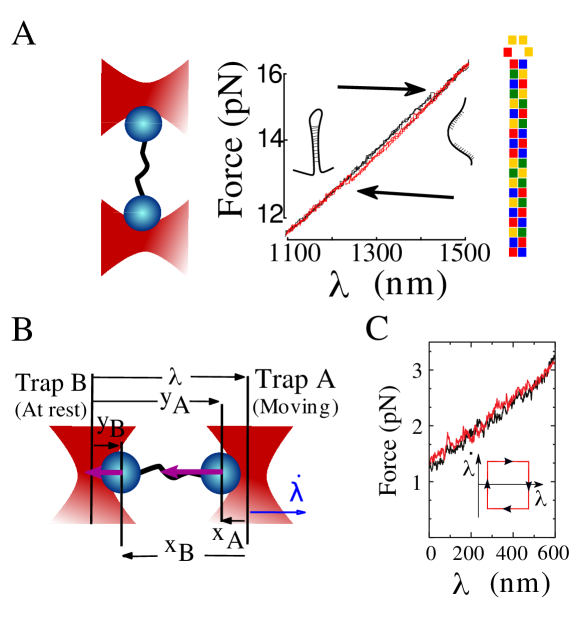
Figure 1:

Pulling experiments with dual-trap optical tweezers. A) Force-distance curves in a pulling experiment on a 20 bp hairpin with our dual-trap setup. A molecular tether is attached between two trapped beads. By increasing the distance, $\lambda$, between the traps the tether is stretched or released until some thermally activated reaction is triggered, e.g. the unfolding or folding of a DNA hairpin, and detected as a force jump (black arrows). The small force jump (0.2 pN) is due to the low-trap stiffness of our dual-trap setup ($\simeq$0.02 pN/nm). Inset: scheme of the hairpin with color-coded sequence (A/T: yellow/green, G/C: red/blue). B) Pulling experiments in a dual-trap setup where trap A is moved at speed $\dot{\lambda}$ and trap B is at rest with respect to water. $\lambda$ is the control parameter, $y_{A}$ and $y_{B}$ are the configurational variables with respect to the moving trap A while $x_{A}$ and $x_{B}$ are the configurational variables with respect to the trap at rest (trap B). C) pulling curves (red stretching, black releasing) for a 3kb ds-DNA tether in a dual-trap setup. Inset: the cyclic pulling protocol used in the experiments.

Caption of Figure 2

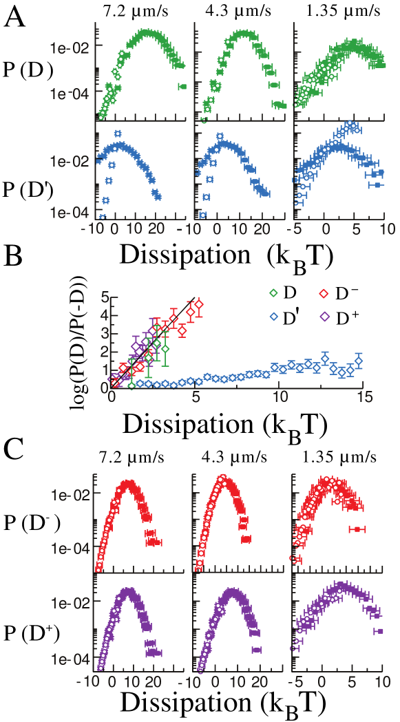
Figure 2:

Work Distributions. Work statistics obtained on cyclic protocols with a 200 nm excursion with different pulling speeds (columns). Four different work observables are considered. In each case the solid points are direct work measurements (l.h.s. of Eq. (27)). In order to improve statistics these distributions are calculated as the convolution of the distribution of the work performed while stretching with that performed while releasing. For that we took all forward and reverse work values $W_{F},W_{R}$ and combined them $W=W_{F}+W_{R}$ in order to get a joint work distribution for the cycle. Open symbols are the reconstructed histogram (r.h.s. of Eq. (27)). Different columns refer to different pulling speeds,$\dot{\lambda}$ , as shown on top. A) Comparison of the measured and reconstructed distributions according to the two definitions of Eq. (25) ($D,D^{\prime}$). The distribution for $D$ satisfies the CFR Eq.(27), i.e. the measured and reconstructed distributions superimpose. The distribution for $D^{\prime}$ does not satisfy it. Horizontal error bars represent the systematic error in work measurements, while vertical error bars denote statistical errors. B) The CFR, Eq. (27) is satisfied within the experimental error for $D,D^{+}$ and $D^{-}$ but not for $D^{\prime}$. C) Comparison between the measured and reconstructed distributions for $D^{-}$ and $D^{+}$ (Eq.(28) and Eq. (29)) both of which satisfy the CFR. Horizontal error bars represent the systematic error in work measurements, while vertical error bars denote statistical errors.

Caption for Figure 3

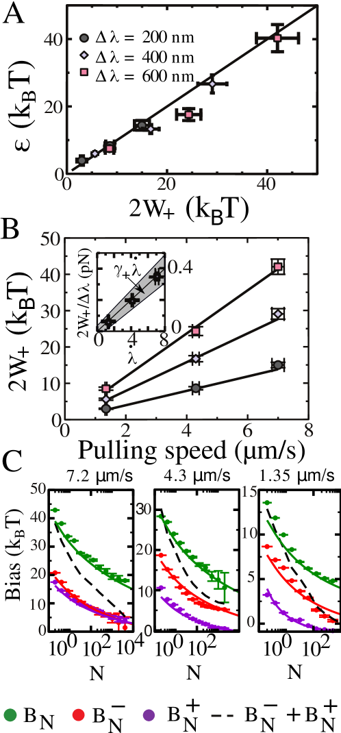
Figure 3:

Bias in unidirectional free energy estimators. A) Error ($\mathcal{E}$) on free energy estimates Eq. (12) committed by using JE for $W^{\prime}$. Circles, diamonds and squares refer to excursions of 200 nm, 400 nm and 600 nm. Three different pulling speeds were considered in each case. Note that in this case work is evaluated over closed cycles ($\Delta G=0$) and the error is defined as: $\mathcal{E}=-\beta^{-1}\log\langle e^{-\beta W^{\prime}}\rangle$. B) $\langle W^{+}\rangle$ displays a bilinear dependence on pulling speed $\dot{\lambda}$ (Main Figure) and $\Delta\lambda$ (Inset) as expected from Eq. (17). Continuous lines are linear fits to the experimental results which contains a single fitting parameter. The shaded area in the inset corresponds to the region within one standard deviation from the expected value of $\langle W^{+}\rangle$ based on equilibrium measurements of $\gamma_{+}$ (see Section 4,5 in the SI). C) Experimental bias measurements from the cycles shown in Fig. 1C. The plots show the bias (Eqs. (22),(23)) as a function of the number of work measurements, $N$. The three plots correspond to different pulling speeds (7.2 $\mu$m/s, 4.3 $\mu$m/s, 1.35 $\mu$m/s). Interestingly $B^{-}_{N}\ll B_{N}$ which guarantees faster convergence of free energy estimates. Moreover $B_{N}$ is also larger than the sum $B^{-}+B^{+}$ (dashed line) i.e. the bias is superadditive (cf. Eq. (24)). The error bars represent the statistical error on free energy determination, not including systematic calibration errors in force and distance. Continuous lines show the theoretical predictions from Ref. [28] for Gaussian work distributions. Note that these are not fits but predictions which only use the mean dissipation as input parameter.

Caption for Figure 4

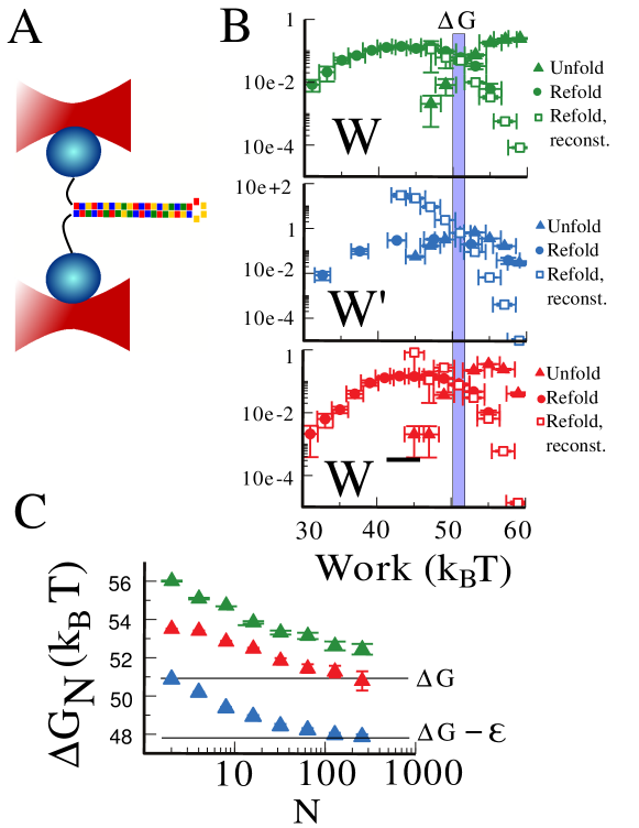
Figure 4:

Work measurements on a DNA hairpin. A)Scheme of the experimental setup (beads and hairpin not to scale). The hairpin is presented with color-coded sequence (A/T: yellow/green, G/C: red/blue). B) Work measurements upon unfolding and refolding according to three different work definitions: $W$ (upper panel), $W^{\prime}$ (central panel) and $W^{-}$ (lower panel). In this experiment pulling speed was $0.96\pm 0.02$ $\mu$m/s. Open symbols show an estimate of the refolding work distributions reconstructed from the unfolding distribution via the CFR (Eq. (26)). $W$ and $W^{-}$ fulfill the fluctuation theorem while $W^{\prime}$ does not. Horizontal error bars represent the systematic error on work measurements, while vertical error bars denote statistical errors. The contribution of trap, handles and single stranded DNA have been removed as detailed in [6]. C) Unidirectional estimates for the free energy from the unfolding work distribution. The optimal estimator based on $W^{-}$ (red) converges to the correct value $\Delta G_{0}=51$ $K_{B}$T as measured from bi-directional estimates. The estimator based on $W$ (green) shows a larger bias and overestimates the free energy by $\simeq 1\,\,K_{B}T$. The estimator based on $W^{\prime}$ (blue) converges to a wrong free energy difference ($\Delta G-\mathcal{E}$) which is $\simeq 3$ $K_{B}T$ below the correct value, against the second law. Note that the error committed by using $W$ is due to finite-size effects and decreases when more unfolding curves are measured. In contrast the error committed by using $W^{\prime}$ remains finite for all sample sizes. The error bars represent the statistical error on free energy determination and do not include the systematic error due to force and distance calibrations.

Caption for Figure 5

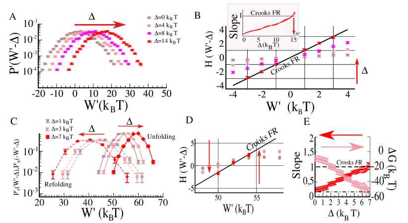
Figure 5:

Inference of $P(W)$ from partial work measurements in the symmetric case. A) The distribution $P^{\prime}(W^{\prime})$ in the case of the dsDNA tether, for the work measured in the wrong trap, $W^{\prime}$. The distribution does not fulfill the CFR. To recover the correct work distribution $P(W)$, $W^{\prime}$ is shifted by a constant amount $\Delta$. The shifted distribution is tested for the CFR by defining the function: $H(W^{\prime})=\log(P^{\prime}(W^{\prime}-\Delta)/P^{\prime}(-W^{\prime}-\Delta))$. The prediction by the CFR is $H(W^{\prime})=\beta\left(W^{\prime}-\Delta G\right)$ which can be tested by determining the $H$ function. B) Evolution of $H(W^{\prime})$ as a function of $W^{\prime}$ for different values of $\Delta$. The value $\Delta^{*}$ for which the slope of $H(W^{\prime})$ is equal to one (work being measured in $K_{B}T$ units) determines the correct work distribution $P(W)$ ($\Delta\simeq 15$, inset). C) In the case of bidirectional measurements both the forward and the reverse work distributions $P^{\prime}_{F}(W^{\prime}),P^{\prime}_{R}(-W^{\prime})$ are shifted by an amount $\Delta$ in opposite directions. D) Evolution of the function $H=\log(P_{F}^{\prime}(W^{\prime}-\Delta)/P_{R}^{\prime}(-W^{\prime}-\Delta))$ as a function of $\Delta$. Again the CFR predicts $H$ should be linear in $W^{\prime}$ with slope one. E) Inference of the correct work distributions and $\Delta G$ measurement. For each value of $\Delta$ a linear fit $A(\Delta)W+B(\Delta)$ to $H$ is performed. The value $\Delta^{*}$ for which $A(\Delta^{*})=1$ ($\Delta^{*}\simeq 7$ in the figure), is the shift needed in order to recover the full work distribution $P(W)$ from partial work measurements in the wrong trap. Moreover the CFR implies $B(\Delta^{*})=-\Delta G$ ($\Delta G\simeq 60K_{B}T$).

Caption for Figure 6

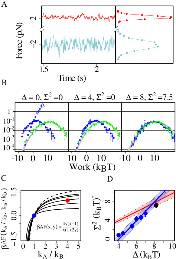
Figure 6:

Inference of $P(W)$ from partial work measurements in the asymmetric case. (A) Equilibrium force distributions at $2$pN for the 3kb ds-DNA tether measured in an asymmetric dual-trap setup ($k_{A}=0.012$ pN/nm,$k_{B}=0.003$ pN/nm,$k_{m}=0.0027$ pN/nm). (B) Convolution of $P^{\prime}(W^{\prime})$ with different Gaussian distributions corresponding to different pairs $\Delta,\Sigma$.We show $P^{\prime}(W)$ (blue filled circles), $P^{\prime}(-W)\exp(\beta W)$ (blue empty circles), $P(W)$ (green filled circles). Among all different $P_{\Delta,\Sigma}$ only one matches the correct work distribution $P(W)$, i.e. only one reconstructed distribution is physically correct (rightmost graph, with $\Delta=7.5$ $K_{B}$T, $\Sigma^{2}=8$ ($K_{B}$T$)^{2}$). In this situation the inference cannot rest on the CFR alone, and additional information is required to infer $P(W)$. (C) Asymmetry factor (AF) as a function of $x=k_{A}/k_{B}$ for different values of $y=k_{m}/k_{B}$. The blue (red) circles indicate the symmetric ($AF=0$) and asymmetric ($AF\simeq 1$) cases respectively. (D) The AF defined by $\Sigma^{2}=AF\times\Delta$ (red line) and the CFR invariance $\Delta=\Delta^{*}+\phi,\Sigma^{2}=\Sigma^{*2}+2\phi K_{B}T$ for any $\phi$ (blue line), do select a narrow range of possible pairs ($\Delta$,$\Sigma$) at the intersection between the blue and red lines. The intersection region is compatible with the parameters ($\Delta$ =8 $K_{B}$T, $\Sigma^{2}$ =7.2 ($K_{B}$T)² ) describing the true correct work distribution $P(W)$ (black point).

See pages - of SI.pdf

References

- [1] Hummer G, Szabo A (2001) Free energy reconstruction from nonequilibrium single-molecule pulling experiments. Proceedings of the National Academy of Sciences 98:3658–3661.
- [2] Hummer G, Szabo A (2010) Free energy profiles from single-molecule pulling experiments. Proceedings of the National Academy of Sciences 107:21441–21446.
- [3] Liphardt J, Dumont S, Smith SB, Tinoco I, Bustamante C (2002) Equilibrium information from nonequilibrium measurements in an experimental test of jarzynski’s equality. Science 296:1832–1835.
- [4] D. Collin, et al. (2005) Verification of the Crooks fluctuation theorem and recovery of RNA folding free energies. Nature 437:231–234.
- [5] Gupta A, et al. (2011) Experimental validation of free energy-landscape reconstruction from non-equilibrium single-molecule force spectroscopy measurements. Nature Physics 7:631–634.
- [6] Alemany A, Mossa A, Junier I, Ritort F (2012) Experimental free energy measurements of kinetic molecular states using fluctuation theorems. Nature Physics 8:688–694.
- [7] Dhakal S, et al. (2010) Coexistence of an ILPR i-motif and a partially folded structure with comparable mechanical stability revealed at the single-molecule level. Journal of the American Chemical Society 132:8991–8997.
- [8] Dhakal S, et al. (2013) Structural and mechanical properties of individual human telomeric G-quadruplexes in molecularly crowded solutions. Nucleic Acids Research 41:3915–3923.
- [9] Cecconi C, Shank E, Bustamante C, Marqusee S (2005) Direct observation of the three-state folding of a single protein molecule. Science 309:2057–2060.
- [10] Shank E, Cecconi C, Dill J, Marqusee S, Bustamante C (2010) The folding cooperativity of a protein is controlled by its chain topology. Nature 465:637–640.
- [11] Gebhardt J, Bornschlögl T, Rief M (2010) Full distance-resolved folding energy landscape of one single protein molecule. Proceedings of the National Academy of Sciences 107:2013–2018.
- [12] Yu H, et al. (2012) Energy landscape analysis of native folding of the prion protein yields the diffusion constant, transition path time, and rates. Proceedings of the National Academy of Sciences 109:14452–14457.
- [13] Harris N, Song Y, Kiang C (2007) Experimental free energy surface reconstruction from single-molecule force spectroscopy using jarzynski’s equality. Physical Review Letters 99:68101–68104.
- [14] Bizzarri A, Cannistraro S (2010) Free energy evaluation of the p53-mdm2 complex from unbinding work measured by dynamic force spectroscopy. Phys. Chem. Chem. Phys. 13:2738–2743.
- [15] Jarzynski C (1997) Nonequilibrium equality for free energy differences. Physical Review Letters 78:2690–2693.
- [16] Crooks GE (1999) Entropy production fluctuation theorem and the nonequilibrium work relation for free energy differences. Physical Review E 60:2721–2726.
- [17] Douarche F, Ciliberto S, Petrosyan A (2005) Estimate of the free energy difference in mechanical systems from work fluctuations: experiments and models. Journal of Statistical Mechanics: Theory and Experiment 09:P09011
- [18] Mossa A, de Lorenzo S, Huguet JM, Ritort F (2009) Measurement of work in single-molecule pulling experiments. The Journal of Chemical Physics 130:234116–234125.
- [19] Alemany A, Ribezzi-Crivellari M, Ritort F (2011) in Nonequilibrium Statistical Physics of Small Systems: Fluctuation Relations and Beyond, eds Klages R, Just W, Jarzynski C (Wiley-VCH, Weinheim) pp 155–179.
- [20] van Mameren J, et al. (2008) Counting rad51 proteins disassembling from nucleoprotein filaments under tension. Nature 457:745–748.
- [21] Cisse I, Mangeol P, Bockelmann U (2011) in Single Molecule Analysis, eds Peterman EJG, Wuite GJL (Humana Press, New York) pp 45-61.
- [22] Moffitt J, Chemla Y, Izhaky D, Bustamante C (2006) Differential detection of dual traps improves the spatial resolution of optical tweezers. Proceedings of the National Academy of Sciences 103:9006–9011.
- [23] Speck T, Mehl J, Seifert U (2008) Role of external flow and frame invariance in stochastic thermodynamics. Physical Review Letters 100:178302–178305.
- [24] Mazonka O, Jarzynski C (1999) Exactly solvable model illustrating far-from-equilibrium predictions. arXiv preprint cond-mat/9912121.
- [25] Wang G, Sevick EM, Mittag E, Searles DJ, Evans DJ (2002) Experimental demonstration of violations of the second law of thermodynamics for small systems and short time scales. Physical Review Letters 89:50601–50604.
- [26] Meiners JC, Quake SR (1999) Direct measurement of hydrodynamic cross correlations between two particles in an external potential. Physical Review Letters 82:2211–2214.
- [27] Gore J, Ritort F, Bustamante C (2003) Bias and error in estimates of equilibrium free energy differences from nonequilibrium measurements. Proceedings of the National Academy of Sciences 100:12564–12569.
- [28] Palassini M, Ritort F (2011) Improving free energy estimates from unidirectional work measurements: theory and experiment. Physical Review Letters 107:60601.
- [29] Ritort F, Bustamante C, Tinoco I (2002) A two-state kinetic model for the unfolding of single molecules by mechanical force. Proceedings of the National Academy of Sciences 99:13544–13548.
- [30] Jarzynski C (2006) Rare events and the convergence of exponentially averaged work values. Phys. Rev. E 73:046105–046114.
- [31] Ribezzi-Crivellari M, Ritort F (2012) Force spectroscopy with dual-trap optical tweezers: Molecular stiffness measurements and coupled fluctuations analysis. Biophysical journal 103:1919–1928.
- [32] Ribezzi-Crivellari M, Huguet JM, Ritort F (2013) Counter-propagating dual-trap optical tweezers based on linear momentum conservation. Review of Scientific Instruments 84:043104–043104.
- [33] Forns N, De Lorenzo S, Manosas M, Hayashi K, Huguet JM, Ritort F (2011) Improving signal/noise resolution in single-molecule experiments using molecular constructs with short handles. Biophysical journal 100:1765–1774.