ABSTRACT.

Quantum capacity, the ultimate transmission rate of quantum communication, is characterized by regularized coherent information. In this work, we reformulate approximations of the quantum capacity by operator space norms and give both upper and lower estimates on quantum capacity and potential quantum capacity using complex interpolation techniques from operator space theory. Upper bounds are obtained by a comparison inequality for Rényi entropies. Analyzing the maximally entangled state for the whole system and for error-free subsystems provides lower bounds for the “one-shot” quantum capacity. These two results combined give upper and lower bounds on quantum capacity for our “nice” classes of channels, which differ only up to a factor $2$, independent of the dimension. The estimates are discussed for certain classes of channels, including group channels, generalized Pauli channels and other high-dimensional channels.

1. Introduction

The aim of quantum Shannon theory is to extend Shannon’s information theory, formulated in his landmark paper [47], and provide the proper framework in the context of quantum mechanics, including non-locality [4, 21]. In recent decades, vast progress has been made in extending Shannon’s theory for quantum channels and their capacities. Moreover, the role of different resources such as entanglement, transmission of classical and quantum bits and their interaction has significantly improved (see e.g. [1, 14, 16]). A surprising but important feature in quantum Shannon theory is the variety of capacities associated with a quantum channel. For instance, the classical capacity [31, 46] describes the capability of classical information transmission through a quantum channel; entanglement-assisted classical capacity [6] considers classical transmission using additional entanglement accessible to the sender Alice and the receiver Bob. One big success in quantum information theory is the quantum capacity theorem proved by Lloyd [40], Shor [48] and Devetak [13] with increasing standards of rigor. It demonstrates that the quantum capacity $Q(\Phi)$ of a channel $\Phi$, as the ultimate capability of $\Phi$ to transmit quantum information, is characterized by the regularized coherent information as follows:

$$Q(\Phi)\hskip 2.84544pt=\hskip 2.84544pt\lim_{k\to\infty}\frac{Q^{(1)}(\Phi^{\otimes k})}{k}\hskip 2.84544pt,\hskip 2.84544ptQ^{(1)}(\Phi)\hskip 2.84544pt=\hskip 2.84544pt\max_{\rho\hskip 2.84544pt\text{\tiny pure}}I_{c}(A\rangle B)_{\sigma}\hskip 2.84544pt,$$ (1.1)

where $\sigma^{AB}=id_{A}\otimes\Phi(\rho^{AA^{\prime}})$ and the maximum runs over all pure bipartite state $\rho^{AA^{\prime}}$. $I_{c}(A\rangle B)_{\sigma}$ is the coherent information of bipartite $\sigma$ given by $H(\sigma^{B})-H(\sigma^{AB})$, with $H(\sigma)=-tr(\sigma\log\sigma)$ being the von Neumann entropy, and $Q^{(1)}$ is the “one-shot” quantum capacity. Let us also recall that the negative cb-entropy (also called the reverse coherent information) of a channel $\Phi$ is defined similarly as ${-S_{cb}(\Phi)=\max_{\rho}H(A)_{\rho}-H(AB)_{\rho}}$ (see Section $2$ for formal definitions).

Despite of this impressive theoretical success, there are few classes of quantum channels which have a closed, computable formula for the quantum capacity. The mathematical reason is the necessity to consider the limit in (1.1), the so-called regularization, which amounts to making calculations for channels with arbitrary large inputs and outputs. It is known that for qubit depolarizing channels the regularization is strictly greater than the “one-shot” expression [17, 50]. Moreover it was proved in [12] that for any $k\in\mathbb{N}$, there exists a channel $\Phi$ such that the regularization of $k$ uses of $\Phi$ is one, but adding one more copy makes it positive, i.e. ${Q^{(1)}(\Phi^{\otimes(k+1)})>Q^{(1)}(\Phi^{\otimes k})=0}$. As of today, calculation of quantum capacities is possible only for specific channels [5, 11, 26]. Devetak and Shor in [16] proved that $Q=Q^{(1)}$ for degradable channels, those for which the environment can be retrieved from Bob’s output with the help of another channel. Hence regularization is not necessary for degradable channels. For non-degradable channels, little is known about the exact value of quantum capacity. Several different methods have been introduced to give estimates on particular or general channels [32, 49, 51, 52, 57].

The aim of this work is to introduce complex interpolation techniques to estimate the quantum capacity $Q$ from above and below for large, nice classes of channels. The upper and lower bounds only differ by a factor of $2$. These in general non-degradable channels can be viewed as perturbations of the so-called conditional expectations, projections onto $C^{*}$-subalgebras. In finite dimensions, conditional expectations are direct sums of partial traces, hence they have clear capacity formula by observations of Fukuda and Wolf in [24]. Based on that, we observe a “comparison property” on entropy and capacity on our nice class of channels. Related estimates for the potential quantum capacity and the quantum dynamic capacity region also follow from the “comparison property”. Moreover, with similar assumptions we prove a formula for the negative cb-entropy.

Here we briefly formulate our results for certain random unitary channels which fall in our nice class. Let $G$ be a finite group of order $|G|=n$ and the left regular representation given by $\lambda(g)(e_{h})=e_{gh}$ on Hilbert space $\ell_{2}(G)\cong l_{2}^{n}$. Here $e_{g}(h)=\delta_{g,h}$ are the standard unit vectors for $\ell_{2}(G)$. There is also a right regular representation ${r(g)(e_{h})=e_{hg^{-1}}}$. The group von Neumann algebra is $L(G)={\rm span}\{\lambda(g)|g\in G\}$ with commutant ${L(G)^{\prime}=\{T|\hskip 2.84544pt\forall{x\in L(G)}\hskip 2.84544pt,Tx=xT\}}$ given by the right regular representation ${L(G)^{\prime}=R(G)={\rm span}\{r(g)|g\in G\}}$ (see e.g. [53]). Given a function $f:G\to{\mathbb{C}}$ with $f(g)\hskip 2.84544pt\geq\hskip 2.84544pt0$ and $\sum_{g}f(g)=n$, we may define the channel

$$\theta_{f}(\rho)\hskip 2.84544pt=\hskip 2.84544pt\frac{1}{n}\sum_{g}f(g)\lambda(g)\rho\lambda(g)^{*}\hskip 2.84544pt.$$ (1.2)

In general, such a random unitary channel is not degradable unless $G$ is abelian. $L(G)$ is a finite dimensional $C^{*}$-algebra and hence admits a decomposition $L(G)=\oplus_{k}M_{n_{k}}$ into matrix blocks, given by a complete list of irreducible representations. We obtain the following estimates for the quantum capacity:

Theorem 1.1.

Let $G$ be a finite group such that ${L(G)=\oplus_{k}M_{n_{k}}}$, and $\theta_{f}$ defined as above. Then

$$\max\{\log(\max_{k}n_{k}),-S_{cb}(\theta_{f})\} \hskip 2.84544pt\leq\hskip 2.84544ptQ^{(1)}(\theta_{f})\hskip 2.84544pt\leq\hskip 2.84544ptQ(\theta_{f})\hskip 2.84544pt\leq\hskip 2.84544pt\log(\max_{k}n_{k})+(-S_{cb}(\theta_{f}))\hskip 2.84544pt,$$ (1.3)

$$-S_{cb}(\theta_{f}) =\log n-H(\frac{1}{n}f).$$ (1.4)

Here $H(\frac{1}{n}f)=-\sum_{g}\frac{f(g)}{n}\log\frac{f(g)}{n}$ is the Shannon entropy. The formula for the cb-entropy of (quantum) group channels has been discovered in the unpublished paper [34] (reproved here), a common source of inspiration for this work and [11]. The upper bound tackles, up to a factor 2, the problem of regularization for this class of non-degradable channels. Our results are particularly striking for non-abelian $G$ with $\max_{k}n_{k}\ll|G|^{1/2}$. Additionally, Theorem (1.1) holds verbatim for quantum groups. We have two motivations for considering quantum groups. First, quantum groups provide new examples of channels with Kraus operators which are neither unitaries nor projections. Second, some variations of quantum group operations relate to Kitaev’s work [38] on anyons. It appears that there is an interesting link between representation theory and capacity.

Our proof relies heavily on operator space tools, in particular complex interpolation. The connection between operator spaces and quantum information has long been noted. In particular, the additivity of the cb-entropy can be derived by differentiating completely bounded norms [15]. In [27] Gupta and Wilde used the same completely bounded norm to prove the strong converse of entanglement-assisted classical capacity. Junge and Palazuelos found a reformulation of entanglement-assisted classical capacity and Holevo capacity in terms of the completely $p$-summing norm [36]. Based on this, they also gave a super-additivity example of $d$-restricted entanglement-assisted classical capacity [35]. Our work discovers connections between quantum capacity and operator space structures and introduce interpolation technique to estimate the Rényi entropy and information measures.

We organize this work as follows. The next section reviews basic definitions about channels and capacities. In Section 3, we state our main theorem and derive our upper bounds based on the “comparison property”

$$\|(id\otimes\theta_{1})(\rho)\|_{p}\hskip 2.84544pt\leq\hskip 2.84544pt\|(id\otimes\theta_{f})(\rho)\|_{p}\hskip 2.84544pt\leq\hskip 2.84544pt\|f\|_{p}\|(id\otimes\theta_{1})(\rho)\|_{p}\hskip 2.84544pt,$$

where $\parallel\!\cdot\!\parallel_{p}$ denotes the Schatten-$p$ norm. This section provide the basic idea of our estimates, postponing operator space terminology and proof. In Section 4 we deliver basic operator space and interpolation theory necessary for the rest of the paper. Section 5 introduces the Stinespring space of a channel and its connection to quantum capacity. Section 6 is devoted to the proof of the “comparison property”. Section 7 discusses cb-entropy and combined upper and lower bounds. Section 8 provides six examples including the group channels we see above.

2. Preliminaries

2.1. States and channels

We denote by $B(H)$ the space of bounded operators on Hilbert space $H$. In this paper, we restrict oursevles to finite dimensional Hilbert spaces and write $\displaystyle\dim H=|H|.$ Sometimes we also use the matrix algebra $M_{n}\cong B(l^{n}_{2})$ where $l^{n}_{2}$ is the standard $n$-dimensional Hilbert space. For $1\leq p<\infty$, the Schatten-$p$ norm of an operator $a\in B(H)$ is defined as

$$\parallel\!a\!\parallel_{p}=tr((a^{*}a)^{\frac{p}{2}})^{\frac{1}{p}}\hskip 2.84544pt,$$

where “$tr$” is the standard trace on matrix algebra. In particular, $p=\infty$ denotes the usual operator norm, and $p=1$ is called the trace class norm. We denote $S_{p}(H)$ (or $S^{n}_{p}$) as the Banach space $B(H)$ (respectively $M_{n}$) equipped with the Schatten-$p$ norm. A state of the system of Hilbert space $H$ is given by a density operator $\rho\in B(H)$, i.e. $\rho\geq 0,\ {tr(\rho)=1}$. Following the duality between the Schrödinger and Heisenberg pictures, we view the density $\rho$ as an element in the trace class operators $S_{1}(H)$, which is the Banach space pre-dual of $B(H)$. A state is called pure if its density is a rank one projector. Pure states are extreme points of the set of states. The identity operator in $B(H)$ is denoted as $1$ and $\frac{1}{|H|}1$ as a density operator is called the totally mixed state.

We index physical systems by capital letters and the corresponding Hilbert spaces by subscripts. For example, it is common to assume Alice is in hold of system $H_{A^{\prime}}$ and Bob $H_{B}$, whereas $H_{A}$ and $H_{E}$ are the reference system and environment respectively. The bipartite system is denoted as $H_{AB}\cong H_{A}\otimes H_{B}$. For a multipartite state, we use the superscripts to track the systems of the states, i.e. for a state $\rho^{AB}\in S_{1}(H_{AB})$, $\rho^{A}=id_{A}\otimes tr_{B}(\rho^{AB})$ is the reduced density operator on $A$. Here $id_{A}$ is the identity map on $B(H_{A})$ whereas the identity operator in $B(H_{A})$ will be denoted by $1_{A}$, and $tr_{B}$ is the trace on $B(H_{B})$. A pure bipartite state of unit vector $|{\psi}\rangle^{AA^{\prime}}$ is a maximally entangled state if $|{\psi}\rangle=\frac{1}{|H_{A}|}\sum_{i}e^{A}_{i}\otimes e^{A^{\prime}}_{i}$ with two orthogonal bases $\{e^{A}_{i}\}$ and $\{e^{A^{\prime}}_{i}\}$.

A quantum channel from Alice to Bob is mathematically a completely positive and trace preserving (CPTP) map $\displaystyle{\Phi:S_{1}(H_{A^{\prime}})\to S_{1}(H_{B})}$, i.e. $id_{A}\otimes\Phi(\rho^{AA^{\prime}})$ is again a state in $S_{1}(H_{AB})$ for all bipartite states $\rho^{AA^{\prime}}\in S_{1}(H_{AA^{\prime}})$ with any reference systems $H_{A}$. Two equivalent definitions of quantum channels will also be used:

1. Kraus operators: there exists a finite sequence of operators $x_{i}\in B(H_{A^{\prime}},H_{B})$ satisfying $\sum_{i}x_{i}^{*}x_{i}=1_{A^{\prime}}$, s.t. $\displaystyle\Phi(\rho)=\sum_{i}x_{i}\rho x_{i}^{*}$;

2. Stinespring dilation: there exists an environment Hilbert space $H_{E}$ and a partial isometry ${V\in B(H_{A^{\prime}},H_{B}\otimes H_{E})}$ with $V^{*}V=1_{{A^{\prime}}}$, s.t.

   $$\Phi(\rho)=id_{B}\otimes tr_{E}(V\rho V^{*})\hskip 2.84544pt.$$ (2.1)

The Stinespring dilation leads to the complementary channel of $\Phi$:

$$\Phi^{E}(\rho)=tr_{B}\otimes id_{E}(V\rho V^{*})\hskip 2.84544pt,$$

for which the outputs are sent to the environment. A channel $\Phi$ is degradable if there exists another channel $\Psi$ such that $\Phi^{E}=\Psi\circ\Phi$. A well-studied class of degradable channels are Hadamard channels, which have a general form as following:

$$\Phi(\rho)=\sum_{1\leq i,j\leq n}\langle{h_{i}}|\rho|{h_{j}}\rangle\langle k_{i}|k_{j}\rangle e_{i,j}\hskip 2.84544pt,$$

where $\sum_{i\leq n}|{h_{i}}\rangle\langle{h_{i}}|=1$, $|{k_{i}}\rangle$’s are unit vectors and $e_{i,j}$’s are the matrix units. Here and in the following we use the standard bra-ket notation.

2.2. Information measures

Given that $\rho$ is a density matrix, the von Neumann entropy of $\rho$ is closely related to its Schatten $p$-norms as follows,

$$H(\rho)\hskip 2.84544pt=\hskip 2.84544pt-tr(\rho\ln\rho)=\lim_{p\to 1^{+}}\frac{1-\|\rho\|_{p}}{p-1}\hskip 2.84544pt.$$ (2.2)

As a matter of convenience, we use the natural logarithm for the definition of entropy, which differs to the logarithm with base $2$ by a constant scalar $\ln 2$. All the main results hold verbatim if the natural logarithm is replaced by $\log_{2}$, in the usual unit of (qu)bit. For a bipartite state $\rho^{AB}$ the mutual information $I(A:B)_{\rho}$ and the coherent information $I_{c}(A\rangle B)$ are defined as

$$I(A;B)_{\rho}:\hskip 2.84544pt=\hskip 2.84544ptH(A)_{\rho}+H(B)_{\rho}-H(AB)_{\rho}\hskip 2.84544pt\ ,\ \hskip 2.84544ptI_{c}(A\rangle B)_{\rho}:\hskip 2.84544pt=\hskip 2.84544ptH(B)_{\rho}-H(AB)_{\rho}\hskip 2.84544pt,$$

where $H(A)_{\rho}=H(\rho^{A})$, $H(AB)=H(\rho^{AB})$. If the state $\rho$ is clear from the context, the subindex is often omitted.

2.3. Channel capacity

Let us briefly review different quantum channel capacities which will be considered in this paper. Here we only state the rate definition of quantum capacity $Q$ but refer to [59] for similar rate definitions of other capacities. Given a channel $\Phi$, a $(n,m,\epsilon)$-quantum code is a pair of completely positive and trace preserving maps $(\mathcal{C},{\mathcal{D}})$,

$$\mathcal{C}:S_{1}^{m}\to S_{1}(H_{A^{\prime}}^{\otimes n})\ \ \ \ {\mathcal{D}}:S_{1}(H_{B}^{\otimes n})\to S_{1}^{m}\hskip 2.84544pt,$$

such that

$$\parallel\!id_{m}\otimes({\mathcal{D}}\circ{\mathcal{N}}^{\otimes^{n}}\circ\mathcal{C})(\phi)-\phi\!\parallel_{1}\hskip 2.84544pt\leq\hskip 2.84544pt\epsilon\hskip 2.84544pt,$$

where $\phi$ is a maximally entangled state in $S_{1}^{m}\otimes S_{1}^{m}$, and $id_{m}$ is the identity map on $S_{1}^{m}$. The maps $\mathcal{C}$ and ${\mathcal{D}}$ are called the encoding and decoding respectively. A non-negative number $R$ is a achievable rate of quantum communication if for any $\epsilon>0$ there exists an $(n,m,\epsilon)$ code such that $\displaystyle\frac{\ln m}{n}\geq R-\epsilon$. Then the quantum capacity of $\Phi$, denoted $Q(\Phi)$, is defined as the supremum of all achievable rates $R$.

The quantum capacity theorem (also known as the LSD theorem) states that for a quantum channel $\Phi$, the capacity to transmit quantum information is

$$Q(\Phi)=\lim_{k\to\infty}\frac{Q^{(1)}(\Phi^{\otimes k})}{k}\hskip 2.84544pt\ \ ,\ \ Q^{(1)}(\Phi)=\max_{\rho^{AA^{\prime}}\ \text{\tiny pure}}I_{c}(A\rangle B)_{\sigma}\hskip 2.84544pt,$$ (2.3)

where $\sigma^{AB}=id_{A}\otimes\Phi(\rho^{AA^{\prime}})$ is the output of channel. The maximum runs over all pure bipartite states $\rho^{AA^{\prime}}$, and by convexity it is equivalent to consider any bipartite states. We will also be concerned with entanglement-assisted classical capacity denoted by $C_{EA}$. The entanglement-assisted classical capacity theorem [6] shows that for a quantum channel $\Phi$, the capacity to transmit classical information with unlimited entanglement-assistance is

$$C_{EA}(\Phi)\hskip 2.84544pt=\hskip 2.84544pt\max_{\rho_{AA^{\prime}}\ {\tiny pure}}I(A;B)_{\sigma}\hskip 2.84544pt.$$ (2.4)

Again the maximum runs over all pure bipartite inputs $\rho^{AA^{\prime}}$. The potential capacities were introduced in [62] by Winter and Yang to consider the maximal possible superadditivity of capacities. In this paper, we only consider the single-letter potential quantum capacity defined as follows:

$$Q^{(p)}(\Phi)\hskip 2.84544pt=\hskip 2.84544pt\sup_{\Psi}\hskip 2.84544ptQ^{(1)}(\Phi\otimes\Psi)-Q^{(1)}(\Psi)\hskip 2.84544pt,$$ (2.5)

where the maximum runs over arbitrary channel $\Psi$. Note that we use a different notation “$Q^{(p)}$” from “$V^{(1)}$” in [49], respectively “$Q^{(1)}_{p}$” in [62] to save the symbol “$Q_{p}$” for later use. By definition, we have $Q^{(p)}\geq Q\geq Q^{(1)}$. $\Phi$ is strongly additive on $Q^{(1)}$ if $Q^{(p)}=Q^{(1)}$, i.e. $Q^{(1)}(\Phi\otimes\Psi)=Q^{(1)}(\Phi)+Q^{(1)}(\Psi)$ for arbitrary $\Psi$. Another information measure we will consider in this paper is the negative $cb$-entropy introduced in [15]:

$$-S_{cb}(\Phi)\hskip 2.84544pt=\hskip 2.84544pt\max_{\rho^{A^{\prime}A},\hskip 2.84544pt\text{pure}}H(A)_{\sigma}-H(AB)_{\sigma}\hskip 2.84544pt.$$ (2.6)

It is also called reverse coherent information, and an operational meaning is discussed in [25].

Finally, we will apply our estimates to the quantum dynamic region. Hsieh and Wilde introduced the quantum dynamic region $C_{CQE}$ to describes the resources traded off with a quantum channel [60] . “$C$” represents classical information transmission, “$Q$” represents qubit transmission and “$E$” is the entanglement distribution. We refer to their paper [60] and Wilde’s book [59] for a formal definition of $C_{CQE}$. Here we state the quantum dynamic theorem from [60] for the convenience of readers. For a quantum channel $\Phi:S_{1}(H_{A^{\prime}})\to S_{1}(H_{B})$, its dynamic capacity region $C_{CQE}$ is characterized as following:

$$C_{CQE}(\Phi)=\overline{\bigcup^{\infty}_{k=1}\frac{1}{k}C_{CQE}^{(1)}(\Phi^{\otimes k})}\ ,\ \ \ \ \ C_{CQE}^{(1)}\equiv\bigcup_{\sigma}C^{(1)}_{CQE,\sigma}$$

where the overbar indicates the closure of a set. The “one-shot" region $C_{CQE}^{(1)}\subset\mathbb{R}^{3}$ is the union of the “one-shot, one-state" regions $C_{CQE,\sigma}^{(1)}$, which are the sets of all rate triples $(C,Q,E)$ such that:

$$C+2Q\leq I(AX;B)_{\sigma}\hskip 2.84544pt,\ Q+E\leq I(A\rangle BX)_{\sigma}\hskip 2.84544pt,\ C+Q+E \leq I(X;B)_{\sigma}+I(A\rangle BX)_{\sigma}\hskip 2.84544pt.$$

The above entropy quantities are with respect to a classical-quantum state

$$\sigma^{XAB}\hskip 2.84544pt=\hskip 2.84544pt\sum_{x}p_{X}(x)|{x}\rangle\langle{x}|^{X}\otimes(id_{A}\otimes\Phi^{A^{\prime}\to B})(\rho^{AA^{\prime}}_{x})$$

and the states $\rho^{AA^{\prime}}_{x}$ are pure.

2.4. Von Neumann algebras

Let us recall that a von Neumann algebra is a weak^∗-closed ^∗-subalgebra of $B(H)$ for some Hilbert space $H$. We say $\tau$ is a normal faithful trace on the von Neumann algebra $N$ if $\tau:N_{+}\to[0,\infty]$ satisfies

1. $\tau(x+y)=\tau(x)+\tau(y)$;

2. $\tau(u^{*}xu)=\tau(x)$ for all unitaries $u$;

3. $\tau(x)=\sup_{0\leq x\leq y,\tau(y)<\infty}\tau(y)$;

4. $\tau(x)=0$ iff $x=0$.

Here $x,y\in N_{+}=\{z^{*}z|z\in N\}$ is the cone of positive elements. In additional, $\tau$ is called normalized if $\tau(1)=1$. For $1\leq p\leq\infty$, the $L_{p}$-norm with respect to trace $\tau$ is defined by

$$\parallel\!a\!\parallel_{p}\hskip 2.84544pt=\hskip 2.84544pt\tau((a^{*}a)^{\frac{p}{2}})^{\frac{1}{p}}\hskip 2.84544pt,\ \ \ a\in N\hskip 2.84544pt,$$

which is a generalization of Schatten-$p$ norms on $N$. A density $\rho\in N$ is a positive element with trace $\tau(\rho)=1$. In operator algebra literature, a state on $N$ is a unital positive linear functional $\phi:N\to\mathbb{C}$, and again by duality, a state is also given by a density $\rho$ in $N$, i.e. $\phi_{\rho}(T)=tr(\rho T)$.

For a given state $\phi$ on $N$, the GNS construction is given by the triple $(H_{\phi},\pi_{\phi},\xi_{\phi})$. The Hilbert space $H_{\phi}=L_{2}(N,\phi)$ is the completion of $N$ with inner product $(x,y)=\phi(x^{*}y)$ and $\xi_{\phi}=|{1}\rangle$ is given by the corresponding vector of identity in $L_{2}(N,\phi)$. Then the GNS representation $\pi_{\phi}$ is $\pi_{\phi}(x)|{y}\rangle=|{xy}\rangle$. If $\phi$ is a normal faithful state, $\xi_{\phi}$ is also separating, and there exists an anti-linear isometry $J$ such that $JNJ=N^{\prime}$ holds for the commutant. In our case, we call the inclusion $N\subset B(H)$ a standard inclusion if $H\cong L_{2}(N,\phi)$ for some faithful state $\phi$. See Section 5 for more information on standard inclusions.

3. Capacity bounds via comparison theorem

3.1. VN-Channels

We are interested in classes of channels indexed by densities from a von Neumann algebra. Indeed, let $N$ be a von Neumann algebra with a faithful normalized trace $\tau$ and $U\in M_{m}\otimes N$ be a unitary. For each density $f\in N$ we may introduce a channel $\theta_{f}:S_{1}^{m}\to S_{1}^{m}$ as follows:

$$\theta_{f}(\rho)=id_{m}\otimes\tau(U(\rho\otimes f)U^{*})\hskip 2.84544pt,$$ (3.1)

Note that the map (3.1) is completely positive and trace preserving if and only if $f$ is a density. We use the normalized trace on $N$ so that that the identity operator $1$ becomes a density in $N$ (i.e. $\tau(a)=1$). Our main goal is to understand perturbations of quantum capacity on the channel $\theta_{1}$. The channels $\theta_{1}$ were intensively studied for the asymptotic quantum Birkhoff theorem (see [29]). We call $\theta_{f}$ VN-channels. One can understand that $f$, chosen from the von Neumann algebra $N$, is a quantum parameter of $\theta_{f}$. Note that in this setting the dimensions $H_{A^{\prime}}=H_{B}=l_{2}^{m}$ coincide. Our first main theorem is the following comparison property on Schatten-$p$ norms for some nice classes of VN-channels.

Theorem 3.1 (Comparison Theorem).

Let $\theta_{f}$ be the channel defined by (3.1). Assume that $N$ and $U$ satisfy the following assumptions,

1. there exists a subalgebra $M\subset M_{m}$ as a standard inclusion ;

2. the unitary $U$ admits a tensor representation $U=\sum_{i}x_{i}\otimes y_{i}\in M^{\prime}\otimes N$;

3. the operator $B=\sum_{i}|x_{i}\rangle\otimes\langle y_{i}^{*}|\in B(L_{2}(N),L_{2}(M))$ satisfies $BB^{*}=\hskip 2.84544ptid_{L_{2}(M)}$.

Then for any bipartite state $\rho^{AA^{\prime}}$ in $S_{1}(H_{A}\otimes H_{A^{\prime}})$ with some reference system $A$,

$$\|(id_{A}\otimes\theta_{1})(\rho)\|_{p}\hskip 2.84544pt\leq\hskip 2.84544pt\|(id_{A}\otimes\theta_{f})(\rho)\|_{p}\hskip 2.84544pt\leq\hskip 2.84544pt\|f\|_{p}\|(id_{A}\otimes\theta_{1})(\rho)\|_{p}\hskip 2.84544pt$$ (3.2)

holds for $1\leq p\leq\infty$.

The assumptions i), ii), iii) are extracted from several concrete classes of channels, including the group channels and quantum group channels mentioned in the introduction. They are discussed in detials in Section 8.

3.2. Upper estimates via Theorem 3.1

Now we translate the $L_{p}$-estimates (3.2) into capacity bounds. We will prove several capacity bounds assuming the “comparison property” Theorem 3.1. Let us start with an immediate consequence.

Corollary 3.2.

Under the assumptions of Theorem 3.1, denote $\hskip 2.84544pt\sigma^{AB}_{f}=id_{A}\otimes\theta_{f}(\rho^{AA^{\prime}})$ and respectively $\hskip 2.84544pt\sigma^{AB}_{1}=id_{A}\otimes\theta_{1}(\rho^{AA^{\prime}})$ as the outputs. Then the following inequalities hold:

1. $H(AB)_{\sigma_{1}}-\tau(f\ln f)\leq H(AB)_{\sigma_{f}}\leq H(AB)_{\sigma_{1}}$;

2. $I_{c}(A\rangle B)_{\sigma_{f}}\leq I_{c}(A\rangle B)_{\sigma_{1}}+\tau(f\ln f)$;

3. $I(A:B)_{\sigma_{f}}\leq I(A:B)_{\sigma_{1}}+\tau(f\ln f)$.

In particular, if $H_{A}$ is one dimensional, i) implies

$$H(B)_{\sigma_{1}}-\tau(f\ln f)\leq H(B)_{\sigma_{f}}\leq H(B)_{\sigma_{1}}\hskip 2.84544pt.$$

Proof.

Thanks to Theorem 3.1 we have

$$\|\sigma_{1}^{AB}\|_{p}\hskip 2.84544pt\leq\hskip 2.84544pt\|\sigma_{f}^{AB}\|_{p}\hskip 2.84544pt\leq\hskip 2.84544pt\|f\|_{p}\hskip 2.84544pt\|\sigma_{1}^{AB}\|_{p}\hskip 2.84544pt.$$

Taking the derivatives at $p=1$, we deduce that

$$H(AB)_{\sigma_{f}}=\lim_{p\to 1^{+}}\frac{1-\|\sigma_{f}\|_{p}}{p-1}\hskip 2.84544pt\leq\hskip 2.84544pt\lim_{p\to 1^{+}}\frac{1-\|\sigma_{1}\|_{p}}{p-1}=H(AB)_{\sigma_{1}}\hskip 2.84544pt,$$

and conversely

$$H(AB)_{\sigma_{f}} =\lim_{p\to 1^{+}}\frac{1-\|\sigma_{f}\|_{p}}{p-1}\geq\lim_{p\to 1^{+}}\frac{1-\|f\|_{p}\|\sigma_{1}\|_{p}}{p-1}$$

$$=\lim_{p\to 1^{+}}\frac{(1-\|f\|_{p})\|\sigma_{1}\|_{p}+(1-\|\sigma_{1}\|_{p})}{p-1}\geq H(AB)_{\sigma_{1}}-\tau(f\ln f)\hskip 2.84544pt.$$

This yields i). For ii), applying i) for the outputs on $B$ and $AB$ we get

$$I_{c}(A\rangle B)_{\sigma_{f}} =H(B)_{\sigma_{f}}-H(AB)_{\sigma_{f}}$$

$$\leq H(B)_{\sigma_{1}}-H(AB)_{\sigma_{1}}+\tau(f\ln f)=I_{c}(A\rangle B)_{\sigma_{1}}+\tau(f\ln f)\hskip 2.84544pt.$$

Since $I(A:B)_{\sigma_{f}}=H(A)_{\sigma_{f}}+I_{c}(A\rangle B)_{\sigma_{f}}$ and $H(A)_{\sigma_{f}}=H(A)_{\sigma_{1}}$, we prove iii). ∎

Remark 3.3.

It is easy to check that the function $g(p)=\|f\|_{p}$ is differentiable and satisfies ${g^{\prime}(1)=\tau(f\ln f)}$ for finite dimensional $N$. The expression $-\tau(f\ln f)$ may be considered as a von Neumann entropy for normalized traces in von Neumann algebras and closely related to the Fuglede determinant, see e.g. [23, 43]. The normalization $\tau(1)=1$ is used in order to prevent cumbersome constants for the symbol $f=1$. For the reader more familiar with the usual trace on matrices, we note that if $N\subset M_{n}$ and the normalized trace $\tau=\frac{tr}{n}|_{N}$ is the restriction of the normalized trace $\frac{tr}{n}$ on $M_{n}$, then $\frac{1}{n}f$ is a density in $M_{n}$ and

$$\tau(f\ln f)=\ln n-H(\frac{1}{n}f)\hskip 2.84544pt.$$

Corollary 3.4.

Under the assumptions of Theorem 3.1, we have

1. $Q^{(1)}(\theta_{f})\leq Q^{(1)}(\theta_{1})+\tau(f\ln f)$, $Q(\theta_{f})\leq Q(\theta_{1})+\tau(f\ln f)$;

2. $C_{EA}(\theta_{f})\leq C_{EA}(\theta_{1})+\tau(f\ln f)$.

Proof.

Taking the supremums on the second inequality of Corollary 3.2, we obtain the inequality of $Q^{(1)}$. For $Q$, we observe that our assumptions are stable under taking tensor products. More precisely, we have

$$(\theta_{f})^{\otimes k}(\rho^{A^{k}{A^{\prime}}^{k}})\hskip 2.84544pt=\hskip 2.84544ptid_{A^{k}}\otimes\tau^{k}(U^{\otimes k}(\rho\otimes f^{\otimes_{k}}){U^{*}}^{\otimes k})\hskip 2.84544pt,$$

and all assumptions of Theorem 3.1 are satisfied for $N^{\otimes k}$ and $U^{\otimes k}$. Then applying the inequality of $Q^{(1)}$ on $\theta_{f}^{\otimes k}\equiv\theta_{f^{\otimes k}}$

$$Q(\theta_{f})= \lim_{k\to\infty}\frac{1}{k}Q^{(1)}(\theta_{f}^{\otimes k})=\lim_{k\to\infty}\frac{1}{k}Q^{(1)}(\theta_{f^{\otimes k}})\leq\lim_{k\to\infty}\frac{1}{k}[Q^{(1)}(\theta_{1^{\otimes k}})+\tau(f^{\otimes k}\ln f^{\otimes k})]$$

$$= \lim_{k\to\infty}\frac{1}{k}(Q^{(1)}(\theta_{1}^{\otimes k})+k\tau(f\ln f))=\lim_{k\to\infty}\frac{1}{k}Q^{(1)}(\theta_{1}^{\otimes k})+\tau(f\ln f)=Q(\theta_{1})+\tau(f\ln f)\hskip 2.84544pt,$$

which proves i). The assertion ii) follows immediately from the third inequality of Corollary 3.2. ∎

We can prove similar capacity bounds for the potential quantum capacity $Q^{(p)}$. For that, we need suitable $L_{p}$-approximations of the “one-shot” expression $Q^{(1)}$. For a quantum channel ${\Phi:S(H_{A^{\prime}})\to S(H_{B})}$ and $p>1$, we can define the following two families of approximation quantities:

$$Q_{p}^{(1)}(\Phi)=\sup_{\rho\mbox{ \tiny pure}}\frac{\|(id_{A}\otimes\Phi)(\rho^{AA^{\prime}})\|_{p}}{\|\Phi(\rho^{A^{\prime}})\|_{p}}\hskip 2.84544pt,\ \ \ Q_{p,d}^{(1)}(\Phi)=\sup_{\rho^{AA^{\prime}},\hskip 2.84544pt|A|\leq d}\frac{\|(id_{A}\otimes\Phi)(\rho^{AA^{\prime}})\|_{p}}{\|\Phi(\rho^{A^{\prime}})\|_{p}}\hskip 2.84544pt.$$

For a fixed $d$ both expressions are related to $Q^{(1)}$ by differentiation at $p=1$.

Lemma 3.5.

For a quantum channel $\Phi$,

1. $\lim_{p\to 1^{+}}\frac{1}{p-1}(Q_{p}^{(1)}(\Phi)-1)=Q^{(1)}(\Phi)$ ; ii) $\lim_{p\to 1^{+}}\frac{1}{p-1}(Q_{p,d}^{(1)}(\Phi)-1)\leq Q^{(1)}(\Phi)$ .

Proof.

The proof of i) is straightforward by uniform convergence of $\displaystyle\frac{1-\|\rho\|_{p}}{p-1}$ to $H(\rho)$ on the state space. For ii) we purify $\rho_{AA^{\prime}}$ on a system $AA^{\prime}F$ with ${|H_{F}|=|H_{A}||H_{A^{\prime}}|=d|H_{A^{\prime}}|}$ and then apply i),

$$\lim_{p\to 1^{+}}\frac{1}{p-1}(Q_{p,d}^{(1)}(\Phi)-1)\leq\lim_{p\to 1^{+}}\frac{1}{p-1}(Q_{p}^{(1)}(\Phi\otimes tr_{|A^{\prime}|d})-1)=Q^{(1)}(\Phi\otimes tr_{|A^{\prime}|d})=Q^{(1)}(\Phi)\hskip 2.84544pt.$$

∎

Proposition 3.6.

Under the assumptions of Theorem 3.1, we have

$$Q^{(p)}(\theta_{f})\leq\tau(f\ln f)+Q^{(p)}(\theta_{1})\hskip 2.84544pt.$$

Proof.

Let $\Psi:S_{1}(H_{A_{1}^{\prime}})\to S_{1}(H_{B_{1}})$ be an arbitrary channel and $\rho^{AA^{\prime}A_{1}^{\prime}}$ be a purification of the bipartite state $\rho^{A^{\prime}A_{1}^{\prime}}$. Let us denote by $\omega^{AA^{\prime}B_{1}}=id_{AA^{\prime}}\otimes\Psi(\rho^{AA^{\prime}A_{1}^{\prime}})$ and

$${\sigma_{f}^{ABB_{1}}=id_{A}\otimes\theta_{f}\otimes\Psi(\rho^{AA^{\prime}A_{1}^{\prime}})}\ ,\ \sigma_{1}^{ABB_{1}}=id_{A}\otimes\theta_{1}\otimes\Psi(\rho^{AA^{\prime}A_{1}^{\prime}}).$$

Note that $\sigma_{f}^{ABB_{1}}=id_{AB_{1}}\otimes\theta_{f}(\omega_{AA^{\prime}B_{1}})$, then we deduce, with the help of Theorem 3.1, that

$$\|\sigma_{f}^{ABB_{1}}\|_{p} \leq\|f\|_{p}\|\sigma_{1}^{ABB_{1}}\|_{p}\hskip 2.84544pt\leq\hskip 2.84544pt\|f\|_{p}\hskip 2.84544ptQ^{(1)}_{p,d}(\theta_{1}\otimes\Psi)\hskip 2.84544pt\|\sigma_{1}^{BB_{1}}\|_{p}\hskip 2.84544pt\leq\hskip 2.84544pt\|f\|_{p}\hskip 2.84544ptQ^{(1)}_{p,d}(\theta_{1}\otimes\Psi)\hskip 2.84544pt\|\sigma_{f}^{BB_{1}}\|_{p}\hskip 2.84544pt.$$

Here $d=|A|$ and $Q^{(1)}_{p,d}$ appears because $\omega^{AA^{\prime}B_{1}}=id_{AA^{\prime}B_{1}}\otimes\Psi(\rho^{AA^{\prime}A_{1}^{\prime}})$ may not be a pure state. According to Lemma 3.5, differentiating the inequality above yields

$$Q^{(1)}(\theta_{f}\otimes\Psi) \hskip 2.84544pt\leq\hskip 2.84544pt\tau(f\ln f)+Q^{(1)}(\theta_{1}\otimes\Psi)\hskip 2.84544pt\leq\hskip 2.84544pt\tau(f\ln f)+Q^{(p)}(\theta_{1})+Q^{(1)}(\Psi)\hskip 2.84544pt.$$

Since $\Psi$ is arbitrary, we deduce

$$Q^{(p)}(\theta_{f}) =\sup_{\Psi}\ Q^{(1)}(\theta_{f}\otimes\Psi)-Q^{(1)}(\Psi)\leq\tau(f\ln f)+Q^{(p)}(\theta_{1})\hskip 2.84544pt.\qed$$

We conclude this section by the application on the quantum dynamic capacity region. Although it is in general difficult to describe this capacity region exactly, there is a mathematically nice way to characterize the “one-shot, one-state” region $C^{(1)}_{CQE,\sigma}$. Let us consider the cone

$$W\hskip 2.84544pt=\hskip 2.84544pt\{(C,Q,E)\hskip 2.84544pt|\hskip 2.84544pt2Q+C\leq 0,\ Q+E\leq 0,\ Q+E+C\leq 0\}$$

obtained from trading resources, i.e. teleportation, superdense coding and entanglement distribution (see [60] for a detailed explanation). Given an output state

$$\sigma^{XABE}=\sum_{x}p(x)|x\rangle\langle x|^{X}\otimes(1_{A}\otimes V)\rho^{AA^{\prime}}(1_{A}\otimes V^{*})\hskip 2.84544pt$$

where $V$ is the Stinespring partial isometry, we find the “one-shot, one-state” achievable region is

$$C^{(1)}_{CQE,\sigma}=(I(X;B)_{\sigma},\frac{1}{2}I(A;B|X)_{\sigma},-\frac{1}{2}I(A:E|X)_{\sigma})+W\hskip 2.84544pt.$$

Thus, instead of estimating the entire “one-shot” region $C^{(1)}_{CQE}=\cup_{\sigma}C^{(1)}_{CQE,\sigma}$, we may compare the entropy terms $(I(X;B)_{\sigma},\frac{1}{2}I(A;B|X)_{\sigma},-\frac{1}{2}I(A:E|X)_{\sigma})$ for a single $\sigma$.

Proposition 3.7.

Under the assumptions of Theorem 3.1, denote $\tau=\tau(f\ln f)$, we have the following inclusions:

1. For each input $\rho^{XAA^{\prime}}=\sum_{x}p(x)|{x}\rangle\langle{x}|^{X}\otimes\rho_{x}^{AA^{\prime}}$ with $\rho_{x}^{AA^{\prime}}$ pure states,
   $C^{(1)}_{CQE,\sigma_{f}}(\theta_{f})\subset C^{(1)}_{CQE,\sigma_{1}}(\theta_{1})+(\tau,\frac{\tau}{2},\frac{\tau}{2})$;

2. $C^{(1)}_{CQE}(\theta_{f})\subset C^{(1)}_{CQE}(\theta_{1})+(\tau,\frac{\tau}{2},\frac{\tau}{2})$, $C_{CQE}(\theta_{f})\subset C_{CQE}(\theta_{1})+(\tau,\frac{\tau}{2},\frac{\tau}{2})$.

Proof.

Let us first compare the rate triple $\big{(}I(X;B),\hskip 2.84544pt\frac{1}{2}I(A;B|X),\hskip 2.84544pt-\frac{1}{2}I(A;E|X)\big{)}$ between $\sigma_{f}$ and $\sigma_{1}$. We denote them respectively as $(C_{f},Q_{f},E_{f})$ and $(C_{1},Q_{1},E_{1})$. By Corollary 3.2, we have

$$I(X;B)_{\sigma_{f}}\leq\tau+I(X;B)_{\sigma_{1}}\hskip 2.84544pt.$$

Hence $C_{f}=C_{1}+\tau-\alpha_{1}$ for some $\alpha_{1}\hskip 2.84544pt\geq\hskip 2.84544pt0$. Similarly, for $\sigma^{AB}_{x,f}=id_{A}\otimes\Phi(\rho_{x}^{AA^{\prime}})$ we have

$$I(A;B|X)_{\sigma_{f}}\hskip 2.84544pt=\hskip 2.84544pt\sum_{x}p(x)H(\rho^{A}_{x})+\sum_{x}p(x)[H(\sigma^{B}_{x,f})-H(\sigma^{AB}_{x,f})]$$

and

$$I(A;E|X)_{\sigma_{f}}\hskip 2.84544pt=\hskip 2.84544pt\sum_{x}p(x)H(\rho^{A}_{x})+\sum_{x}p(x)[H(\sigma^{E}_{x,f})-H(\sigma^{AE}_{x,f})]\hskip 2.84544pt.$$

Since each $\rho^{AA^{\prime}}_{x}$ is pure we get $H(\sigma^{E}_{x,f})=H(\sigma^{AB}_{x,f})$ and $H(\sigma^{AE}_{x,f})=H(\sigma^{B}_{x,f})$. This means

$$Q_{f}\hskip 2.84544pt=\hskip 2.84544ptQ_{1}+\frac{\tau-\alpha_{2}}{2}\hskip 2.84544pt,\hskip 2.84544ptE_{f}\hskip 2.84544pt=\hskip 2.84544ptE_{1}+\frac{\tau-\alpha_{2}}{2}\hskip 2.84544pt$$

for some $\alpha_{2}\hskip 2.84544pt\geq\hskip 2.84544pt0$. Now we observe that $(-\alpha_{1},-\frac{\alpha_{2}}{2},-\frac{\alpha_{2}}{2})\in W$ because $-\alpha_{1}-\alpha_{2}\hskip 2.84544pt\leq\hskip 2.84544pt0$ and $-\alpha_{2}\leq 0$. Thus we obtain

$$(C_{f},Q_{f},E_{f})\in(\tau,\frac{\tau}{2},\frac{\tau}{2})+(C_{1},Q_{1},E_{1})+W\hskip 2.84544pt.$$

Since $W$ is a cone, $W+W=W$. we get

$$C^{(1)}_{CQE,\sigma_{f}}=(C_{f},Q_{f},E_{f})+W\subset(\tau,\frac{\tau}{2},\frac{\tau}{2})+(C_{1},Q_{1},E_{1})+W+W=(\tau,\frac{\tau}{2},\frac{\tau}{2})+C^{(1)}_{CQE,\sigma_{1}}\hskip 2.84544pt.$$

This concludes the proof of i). For ii), taking the union over all output $\sigma$ implies

$$C^{(1)}_{CQE}(\theta_{f})\subset(\tau,\frac{\tau}{2},\frac{\tau}{2})+C^{(1)}_{CQE}(\theta_{1})\hskip 2.84544pt.$$

For iii), we use again the fact that $\theta_{f}^{\otimes_{k}}\equiv\theta_{f^{\otimes_{k}}}$ is of the same nature as $\theta_{f}$ and hence we deduce that

$$\frac{1}{k}C^{(1)}_{CQE}(\theta_{f}^{\otimes k})\subset\frac{1}{k}[k(\tau,\frac{\tau}{2},\frac{\tau}{2})+C_{CQE}^{(1)}(\theta_{1}^{\otimes k})]=(\tau,\frac{\tau}{2},\frac{\tau}{2})+\frac{1}{k}C_{CQE}^{(1)}(\theta_{1}^{\otimes k})\hskip 2.84544pt.$$

The result follows by taking the union over $k\in{\mathbb{N}}$. ∎

Remark 3.8.

i) All above estimates rely on the special channel $\theta_{1}$. Fortunately, we will see in Section 5 that $\theta_{1}$ is a channels as direct sums of partial trace, which has clear capacity expression depending on the von Neumann algebra $M$. It can also be deduced from [60] that the capacity region of such $\theta_{1}$ is strongly additive, hence it is regularized. Namely, we obtain the following “single-letter upper bound”

$$C_{CQE}(\theta_{f})\subset(\tau,\frac{\tau}{2},\frac{\tau}{2})+{C_{CQE}^{(1)}(\theta_{1})}\hskip 2.84544pt.$$

ii) If in additional $\theta_{f}$ is unital ($\theta_{f}(1)=1$), we find ${(\tau,\frac{\tau}{2},\frac{\tau}{2})\in 2C^{(1)}_{CQE}(\theta_{f})}$. Indeed, we choose the input state $\rho^{AA^{\prime}}$ to be a maximal entangled state, then ${\displaystyle(0,\frac{1}{2}(\ln m+\tau),\frac{1}{2}(-\ln m+\tau))}$ and hence $(\tau,0,0)$, $(0,\frac{\tau}{2},\frac{\tau}{2})$ belong to $C^{(1)}_{CQE}(\theta_{f})$. Our estimate implies a comparison of convex regions often considered in convex geometry and Banach spaces

$$C_{CQE}(\theta_{1})\subset C_{CQE}(\theta_{f})\subset(\tau,\frac{\tau}{2},\frac{\tau}{2})+C_{CQE}(\theta_{1})\subset 3C_{CQE}(\theta_{1})\hskip 2.84544pt.$$

The first inclusion is an immediate consequence of Lemma 6.7.

4. Operator space duality and $L_{p}$-spaces

4.1. Basic operator space

The background on operator space reviewed here is avalible in [20] and [45]. We say X is a (concrete) operator space if $X\subset B(H)$ is a closed subspace for some Hilbert space $H$. The $C^{*}$-algebra $B(H)$ has a natural sequence of matrix norms associated with it: $M_{n}(B(H))=B(H^{\otimes n})$. Then the inclusion $X\subset B(H)$ not only equips $X$ with a Banach space norm, but also a sequence of norms on the vector-valued matrices

$$M_{n}(X)=\{(x_{ij})_{ij}|\hskip 2.84544ptx_{ij}\in X,\forall 1\leq i,j\leq n\}\hskip 2.84544pt.$$

Here we understand $M_{n}(X)\subset M_{n}(B(H))$ as being isometrically embedded. This sequence of matrix norms satisfy Ruan’s Axioms, which are two properties inherited from $M_{n}(B(H))$ (here $1$ denotes the identity operator of $B(H)$):

1. $\text{For any}\ a,b\in M_{n},\ x=(x_{ij})\in M_{n}(X),\$

   $\parallel\!(a\otimes 1)(x_{ij})(b\otimes 1)\!\parallel\leq\parallel\!a\!\parallel_{M_{n}}\parallel\!x\!\parallel_{M_{n}(X)}\parallel\!b\!\parallel_{M_{n}}$;

2. $\text{For any}\ x=(x_{ij})\in M_{n}(X),\ y=(y_{ij})\in M_{m}(X),\$

   $\parallel\!\left(\begin{array}[]{cc}x&0\\ 0&y\end{array}\right)\!\parallel_{M_{n+m}(X)}\leq\max\{\parallel\!x\!\parallel_{M_{n}(X)},\ \parallel\!y\!\parallel_{M_{m}(X)}\}\hskip 2.84544pt.$

An operator space structure is either given by a concrete embedding $X\subset B(H)$ or a sequence of matrix norms satisfying Ruan’s axioms. Thanks to Ruan’s theorem this defines the same category, i.e. every matrix normed space satisfying Ruan’s axioms admits an embedding ${\iota:X\to B(H)}$ which preserves the norms on all levels. A map ${\iota:X\to Y}$ such that ${id_{n}\otimes\iota:M_{n}(X)\to M_{n}(Y)}$ is isometric for all $n$ is called a complete isometry. Basic examples of operator spaces are given by the column space $C_{n}$ and the row space $R_{n}$:

$$C_{n}={\rm span}\{e_{i,1}|1\leq i\leq n\}\subset M_{n},\ \ R_{n}={\rm span}\{e_{1,i}|1\leq i\leq n\}\subset M_{n}\hskip 2.84544pt.$$ (4.1)

Here and in the following $e_{i,j}$ denote the standard matrix unit (with the respect to the computational basis), i.e. the matrix which is $0$ except for the single entry $1$ in $i$-th row and $j$-th column. A basis-free description of the row and column space can be given as follows

$$H^{c}=B({\mathbb{C}},H)\ \ ,\ H^{r}=B(H,{\mathbb{C}})\hskip 2.84544pt.$$ (4.2)

The morphisms between operator spaces are completely bounded maps ($cb$-maps). Given two operator spaces $X,Y$ and a linear map $u:X\to Y$, we say $u$ is completely bounded if the $cb$-norm

$$\|u\|_{cb}\hskip 2.84544pt=\hskip 2.84544pt\sup_{n}\|id_{M_{n}}\otimes u:M_{n}(X)\to M_{n}(Y)\|$$ (4.3)

is finite. The space of completely bounded maps from $X$ to $Y$ is denoted as $CB(X,Y)$. Clearly, $CB(X,Y)$ is a Banach space, even more an operator space equipped with the matrix level structure $M_{n}(CB(X,Y))=CB(X,M_{n}(Y))$. Particularly, ${X^{*}=CB(X,{\mathbb{C}})}$ is called the operator space dual of $X$.

4.2. Haagerup tensor product

Beyond the basic operator space concepts, the Haagerup tensor product is also a key tool in our estimates. Let us recall that for two operator spaces $X\subset B(H)$ and $Y\subset B(K)$, the Haagerup tensor norm is defined on $X\otimes Y$ as

$$\|z\|_{X\otimes_{h}Y}\hskip 2.84544pt=\hskip 2.84544pt\inf_{z=\sum_{k}x_{k}\otimes y_{k}}\|(\sum_{k}x_{k}x_{k}^{*})^{1/2}\|_{B(H)}\|(\sum_{k}y_{k}^{*}y_{k})^{1/2}\|_{B(K)}\hskip 2.84544pt.$$

In many cases we will not be able to provide a concrete embedding $X\subset B(H)$, and then it is better to note that

$$\|(\sum_{k}x_{k}x_{k}^{*})^{1/2}\|\hskip 2.84544pt=\hskip 2.84544pt\|\sum_{k}x_{k}\otimes e_{1,k}\|_{R_{n}(X)}\hskip 2.84544pt,\hskip 2.84544pt\|(\sum_{k}y_{k}^{*}y_{k})^{1/2}\|\hskip 2.84544pt=\hskip 2.84544pt\|\sum_{k}e_{1,k}\otimes y_{k}\|_{C_{n}(X)}\hskip 2.84544pt,$$

where $C_{n}(X),R_{n}(X)\subset M_{n}(X)$ are the $X$-valued column and row spaces. The Haagerup tensor product can recover the operator space structure

$$M_{n}(X)\hskip 2.84544pt=\hskip 2.84544ptC_{n}\otimes_{h}X\otimes_{h}R_{n}\hskip 2.84544pt,\hskip 2.84544pt\ C_{n}(X)=C_{n}\otimes_{h}X\hskip 2.84544pt,\hskip 2.84544ptR_{n}(X)=X\otimes_{h}R_{n}\hskip 2.84544pt,$$

which holds completely isometrically. In particular, we have

$$M_{n}(M_{m}) =C_{n}\otimes_{h}M_{m}\otimes_{h}R_{n}\hskip 2.84544pt=\hskip 2.84544ptM_{mn}$$

$$C_{n}(C_{m}) =C_{n}\otimes_{h}C_{m}=C_{mn}\hskip 2.84544pt,\hskip 2.84544ptR_{n}(R_{m})=R_{m}\otimes_{h}R_{n}=R_{mn}\hskip 2.84544pt.$$

These identifications are also compatible with the general duality relation

$$(X\otimes_{h}Y)^{*}\hskip 2.84544pt=\hskip 2.84544ptX^{*}\otimes_{h}Y^{*}\hskip 2.84544pt.$$

We recall that (see e.g. [20, 45]) $C_{n}^{*}=R_{n}$, $R_{n}^{*}=C_{n}$ holds completely isometrically. This implies

$$M_{n}^{*}=(C_{n}\otimes_{h}R_{n})^{*}=R_{n}\otimes_{h}C_{n}=S_{1}^{n}\ ,\ (S_{1}^{n})^{*}=(R_{n}\otimes_{h}C_{n})^{*}=C_{n}\otimes_{h}R_{n}=M_{n}\hskip 2.84544pt.$$

It is important to note that the columns in $S_{1}^{n}$ carry the operator space structure of $R_{n}$, and the rows in $S_{1}^{n}$ become $C_{n}$. Another fundamental concept is the minimal tensor norm for operator spaces $X\subset B(H)$, $Y\subset B(K)$ given by

$$X\otimes_{\min}Y\subset B(H)\otimes_{\min}B(K)\subset B(H\otimes K)\hskip 2.84544pt,$$

where the second inclusion serves as a definition of the $\min$-norm ($\min$ operator space structure). The connection with the space $CB(X,Y)$ is functorial, i.e. if one of the spaces is finite dimensional then

$$CB(X,Y)\hskip 2.84544pt=\hskip 2.84544ptX^{*}\otimes_{\min}Y$$ (4.4)

holds completely isometrically. The minimal tensor norm is the smallest operator space tensor norm (see [45, 20]).

4.3. Complex interpolation

Let $X_{0}$ and $X_{1}$ be two Banach spaces. We say $X_{0}$ and $X_{1}$ are compatible if there exists a Hausdorff topological vector $X$ such that $X_{0},X_{1}\subset X$ as subspaces. One can define the sum as

$$X_{0}+X_{1}:\hskip 2.84544pt=\hskip 2.84544pt\{x\in X|x=x_{0}+x_{1}\hskip 2.84544pt\text{for some}\hskip 2.84544ptx=X_{0},x_{1}\in X_{1}\}\hskip 2.84544pt,$$

and $X_{0}+X_{1}$ equipped with the norm

$$\parallel\!x\!\parallel_{X_{0}+X_{1}}=\inf_{x=x_{0}+x_{1}}(\parallel\!x_{0}\!\parallel_{X_{0}}+\parallel\!x_{1}\!\parallel_{X_{1}})$$

is again a Banach space. Let us denote by $S=\{z|0\leq Re(z)\leq 1\}$ the classical vertical strip of unit width on the complex plane and $S_{0}=\{z|0<Re(z)<1\}$ its open interior. We will consider the space ${\mathcal{F}}(X_{0},X_{1})$ of all functions $f:S\to X_{0}+X_{1}$, which are bounded and continuous on $S$ and analytic on $S_{0}$, and moreover

$$\{f(it)|t\in\mathbb{R}\}\subset X_{0}\hskip 2.84544pt,\hskip 2.84544pt\{f(1+it)|t\in\mathbb{R}\}\subset X_{1}\hskip 2.84544pt.$$

${\mathcal{F}}(X_{0},X_{1})$ is a Banach space under the norm

$$\parallel\!f\!\parallel_{{\mathcal{F}}}=\max\{\sup_{t\in\mathbb{R}}\parallel\!f(it)\!\parallel_{X_{0}},\sup_{t\in\mathbb{R}}\parallel\!f(1+it)\!\parallel_{X_{1}}\}\hskip 2.84544pt.$$

For $0<\theta<1$, the complex interpolation space $(X_{0},X_{1})_{\theta}$ is defined as a subspace of ${\mathcal{F}}(X_{0},X_{1})$ as follows

$$(X_{0},X_{1})_{\theta}=\{x\in X_{0}+X_{1}|\hskip 2.84544ptx=f(\theta),f\in F(X_{0},X_{1})\}\hskip 2.84544pt.$$

$(X_{0},X_{1})_{\theta}$ is a Banach space equipped with the norm

$$\parallel\!x\!\parallel_{\theta}=\inf\{\parallel\!f\!\parallel_{{\mathcal{F}}}|f(\theta)=x\}\hskip 2.84544pt.$$

For example, the Schatten-$p$ class is the interpolation space of bound operator and trace class

$$S_{p}(H)=(B(H),S_{1}(H))_{\frac{1}{p}}\hskip 2.84544pt.$$

The following Stein’s interpolation theorem (cf. [7]) is a key tool in our analysis.

Theorem 4.1.

Let $(X_{0},X_{1})$ and $(Y_{0},Y_{1})$ be two compatible couples of Banach spaces. Let $\{T_{z}|z\in S\}\subset B(X_{0}+X_{1},Y_{0}+Y_{1})$ be a bounded analytic family of maps such that

$$\{T_{it}|t\in\mathbb{R}\}\subset B(X_{0},Y_{0})\hskip 2.84544pt,\hskip 2.84544pt\{T_{1+it}|t\in\mathbb{R}\}\subset B(X_{1},Y_{1})\hskip 2.84544pt.$$

Suppose $M_{0}=\sup_{t}{\parallel\!T_{it}\!\parallel_{B(X_{0},Y_{0})}}$ and $M_{1}=\sup_{t}{\parallel\!T_{1+it}\!\parallel_{B(X_{1},Y_{1})}}$ are both finite, then $T_{\theta}$ is a bounded linear map from $(X_{0},X_{1})_{\theta}$ to $(Y_{0},Y_{1})_{\theta}$ and

$$\parallel\!T_{\theta}\!\parallel_{B((X_{0},X_{1})_{\theta},(Y_{0},Y_{1})_{\theta})}\leq M_{0}^{1-\theta}M_{1}^{\theta}\hskip 2.84544pt.$$

In particular, when $T$ is a constant map, the above theorem implies

$$\parallel\!T\!\parallel_{B((X_{0},X_{1})_{\theta},(Y_{0},Y_{1})_{\theta})}\leq\parallel\!T\!\parallel_{B(X_{0},Y_{0})}^{1-\theta}\parallel\!T\!\parallel_{B(X_{1},Y_{1})}^{\theta}\hskip 2.84544pt.$$ (4.5)

4.4. Noncommutative $L_{p}$-spaces

Noncommutative $L_{p}$-spaces may be obtained by complex interpolation. Indeed, (for finite dimension $H$) we have

$$S_{p}(H)\hskip 2.84544pt=\hskip 2.84544pt(B(H),S_{1}(H))_{\frac{1}{p}}\hskip 2.84544pt=\hskip 2.84544pt(H^{c}\otimes_{h}H^{r},H^{r}\otimes_{h}H^{c})_{\frac{1}{p}}\hskip 2.84544pt=\hskip 2.84544pt(H^{c},H^{r})_{\frac{1}{p}}\otimes_{h}(H^{r},H^{c})_{\frac{1}{p}}\hskip 2.84544pt.$$

The second equality is an instance of Kouba’s interpolation formula for the Haagerup tensor product (see [7, 44, 45] for more details),

$$(X_{0},X_{1})_{\theta}\otimes_{h}(Y_{0},Y_{1})_{\theta}=(X_{0}\otimes_{h}Y_{0},X_{1}\otimes_{h}Y_{1})_{\theta}\hskip 2.84544pt.$$

We will adapt the notation $H^{c_{p}}=(H^{c},H^{r})_{\frac{1}{p}}$ and $H^{r_{p}}=(H^{r},H^{c})_{\frac{1}{p}}$ for the columns and row in $S_{p}(H)$ respectively. This definition leads to the “little Fubini theorem”

$$H^{c_{p}}\otimes_{h}K^{c_{p}}\hskip 2.84544pt=\hskip 2.84544pt(H\otimes K)^{c_{p}}\hskip 2.84544pt,\hskip 2.84544ptH^{r_{p}}\otimes_{h}K^{r_{p}}\hskip 2.84544pt=\hskip 2.84544pt(H\otimes K)^{r_{p}}\hskip 2.84544pt,$$ (4.6)

for two Hilbert spaces $H$ and $K$. In some instance we will make use of vector-valued $L_{p}$ spaces. For an operator space $X$, we recall Pisier’s definition

$$S_{p}(H,X)\hskip 2.84544pt=\hskip 2.84544ptH^{c_{p}}\otimes_{h}X\otimes_{h}H^{r_{p}}\hskip 2.84544pt.$$

An important special case is given by

$$\|\xi\|_{S_{p}(H_{A},S_{q}(H_{B}))}\hskip 2.84544pt=\hskip 2.84544pt\sup_{\|a\|_{2r}\|b\|_{2r}\leq 1}\|(a\otimes 1_{B})\xi(b\otimes 1_{B})\|_{S_{q}(H_{A}\otimes H_{B})}$$ (4.7)

where $q\leq p$, $1/p+1/r=1/q$ and

$$\|\xi\|_{S_{p}(H_{A},S_{q}(H_{B}))}\hskip 2.84544pt=\hskip 2.84544pt\inf_{\xi=(a\otimes 1_{B})\eta(b\otimes 1_{B})}\|a\|_{2r}\|\eta\|_{S_{q}(H_{A}\otimes H_{B})}\|b\|_{2r}$$

where $q\geq p$, $1/q+1/r=1/p$. It is not difficult to show that for $\xi\hskip 2.84544pt\geq\hskip 2.84544pt0$ it suffices to consider $a=b^{*}\geq 0\in B(H_{A})$ in both cases.

5. Stinespring space and its Operator Space structures

Suppose a channel $\Phi:S_{1}(H_{A^{\prime}})\to S_{1}(H_{B})$ from Alice to Bob has a Stinespring dilation

$$\Phi(\rho)=id_{B}\otimes tr_{E}(V\rho V^{*})\hskip 2.84544pt,$$

where $V:H_{A^{\prime}}\to H_{B}\otimes H_{E}$ is a partial isometry such that $V^{*}V=1_{A^{\prime}}$. Then the Stinespring space of $\Phi$ is defined to be the range of partial isometry $V$:

$$\operatorname{st}(\Phi)\equiv\text{Im}(V)=\{V(h)|\hskip 2.84544pth\in H_{A}\}\subset H_{B}\otimes H_{E}\hskip 2.84544pt.$$

Although the partial isometry $V$ is not unique, different dilations only differ by unitary transformations on $H_{E}$, and hence will not affect the operator space structure of $\operatorname{st}(\Phi)$. The Stinespring space is well-known and has been used instrumentally in disproving the additivity conjecture for the minimal entropy (see [30]). It has become clear that the family of Schatten $p$-norms on $H_{B}\otimes H_{E}$ are related to entropy. In this paper we will go one step further and consider the operator space structure of the Stinespring space. For $1\leq p\leq\infty$, let us denote $\operatorname{st}_{p}(\Phi)$ as the operator subspace $\operatorname{st}(\Phi)$ induced by the following inclusion

$$\operatorname{st}_{p}(\Phi)\subset H_{B}^{c_{p}}\otimes_{h}H_{E}^{r}\hskip 2.84544pt.$$

Let us recall that for two Hilbert space $H$ and $K$,

$$H^{c_{p}}\otimes_{h}K^{r}\hskip 2.84544pt=\hskip 2.84544pt[H^{c}\otimes_{h}K^{r},H^{r}\otimes_{h}K^{r}]_{\frac{1}{p}}\hskip 2.84544pt=\hskip 2.84544ptS_{2p}(K,H)\hskip 2.84544pt.$$

Here $S_{p}(H,K)$ stands for Schatten-$p$ class of operators from $K$ to $H$. Note that the operator space structure here is not usual one (i.e. $H^{c_{2p}}\otimes_{h}K^{r_{2p}}$), see [35] for more details on asymmetric $L_{p}$-spaces.

Lemma 5.1.

Let $\Phi:S_{1}(H_{A^{\prime}})\to S_{1}(H_{B}))$ be a channel with Stinespring dilation isometry $V$. Let $\xi^{AA^{\prime}}$ and $\rho^{AA^{\prime}}=\xi\xi^{*}$ be operators in $B(H_{A}\otimes H_{A^{\prime}})$. Denote ${\eta=(1_{A}\otimes V)\xi}$, then

1. $\|(id_{A}\otimes\Phi)(\rho^{AA^{\prime}})\|_{S_{p}(H_{A}\otimes H_{B})}\hskip 2.84544pt=\hskip 2.84544pt\|\eta\|^{2}_{H_{A}^{c_{p}}\otimes_{h}\operatorname{st}_{p}(\Phi)\otimes_{h}(H_{A^{\prime}}\otimes H_{A})^{r}}$;

2. $\|\Phi(\rho^{A^{\prime}})\|_{S_{p}(H_{B})}\hskip 2.84544pt=\hskip 2.84544pt\|\eta\|^{2}_{\operatorname{st}_{p}(\Phi)\otimes_{h}(H_{A}\otimes H_{A^{\prime}}\otimes H_{A})^{r}}$.

In particular, if $\rho=|\xi\rangle\langle\xi|$ is given by a pure state then $\eta$ belongs to $H_{A}^{c_{p}}\otimes_{h}\operatorname{st}_{p}(\Phi)$ for i) and respectively $\operatorname{st}_{p}(\Phi)\otimes_{h}H_{A}^{r}$ for ii).

Proof.

In this proof, it is important to track the position of vectors and covectors (column vectors and row vectors) in the tensor components. We may assume that $\Phi$ has Kraus operators $\Phi(\rho)=\sum_{i}x_{i}\rho x_{i}^{*}$, and $V=\sum_{i}x_{i}\otimes e_{i,1}$. To specify the tensor components, we denote ${\xi=\sum_{j}|a_{j}^{A}\rangle|h_{j}^{A^{\prime}}\rangle\langle b_{j}^{A}|\langle k_{j}^{A^{\prime}}|}$ where $|a_{j}^{A}\rangle,|b_{j}^{A}\rangle$ are vectors of $H_{A}$ and $|h_{j}^{A^{\prime}}\rangle,|b_{j}^{A^{\prime}}\rangle$ vectors of $H_{A^{\prime}}$. We use the “little Fubini theorem” (4.6)

$$\eta\hskip 2.84544pt=\hskip 2.84544pt\sum_{i=1}^{d}(1_{A}\otimes x_{i})\xi^{AA^{\prime}}\otimes e_{i,1}=\sum_{j,i}|a_{j}^{A}\rangle|x_{i}(h_{j})^{B}\rangle\otimes\langle b_{j}^{A},k_{j}^{A^{\prime}}|\otimes|{i^{E}}\rangle$$

$$\cong\hat{\eta}\equiv\sum_{j}|a_{j}^{A}\rangle\otimes\bigg{(}\sum_{i}|x_{i}(h_{j})^{B}\rangle\otimes\langle i^{E}|\bigg{)}\otimes\langle k_{j}^{A},b_{j}^{A^{\prime}}|\ \ \ \ \ \ \ \text{ (shuffle)}$$

$$\in H_{A}^{c_{p}}\otimes_{h}\operatorname{st}_{p}(\Phi)\otimes_{h}(H_{A}\otimes H_{A^{\prime}})^{r}\subset(H_{A}\otimes H_{B})^{c_{p}}\otimes_{h}(H_{E}\otimes H_{A}\otimes H_{A^{\prime}})^{r}\hskip 2.84544pt,$$

where in the second line above, we first change the role of $E$ system from column to row, and then switch between row vectors $\langle{i^{E}}|$ and $\langle k_{j}^{A},b_{j}^{A^{\prime}}|$. This action is an identification and we get $\hat{\eta}\hat{\eta}^{*}=(id_{A}\otimes\Phi)(\rho_{AA^{\prime}})$. Now the first assertion follows from the fact ${\parallel\!a\!\parallel_{S_{2p}(K,H)}^{2}=\parallel\!aa^{*}\!\parallel_{S_{p}(H)}}$. For ii), we first note that

$$\|\Phi(\rho_{A^{\prime}})\|_{p}\hskip 2.84544pt=\hskip 2.84544pt\|(tr_{A}\otimes id_{B})\circ\Phi(\rho^{AA^{\prime}})\|_{p}\hskip 2.84544pt=\hskip 2.84544pt\|tr_{A}\otimes id_{B}(\hat{\eta}\hat{\eta}^{*})\|_{p}\hskip 2.84544pt.$$

The trace on $A$ make $H_{A}$ row vector to the right of $\operatorname{st}_{p}(\Phi)$. Namely,

$$\eta\cong\tilde{\eta}\equiv\sum_{j}\bigg{(}\sum_{i}|x_{i}(h_{j})^{B}\rangle\otimes\langle i^{E}|\bigg{)}\otimes\langle a_{j}^{A}|\otimes\langle k_{j}^{A},b_{j}^{A^{\prime}}|\ \ \ \ \ \ \ \text{ (shuffle)}$$

$$\in\operatorname{st}_{p}(\Phi)\otimes_{h}(H_{A}\otimes H_{A}\otimes H_{A^{\prime}})^{r}\subset H_{B}^{c_{p}}\otimes_{h}(H_{E}\otimes H_{A}\otimes H_{A}\otimes H_{A^{\prime}})^{r}\hskip 2.84544pt,$$

When $\rho\in S_{1}(H_{A^{\prime}})$ is a pure state, the right part $(H_{A}\otimes H_{A^{\prime}})^{r}$ become trivial, which yields the last assertion.∎

Let us recall another definition from the theory of noncommutative vector-valued $L_{p}$ space. For an operator space $X$ we use

$$C_{p}^{n}(X)\hskip 2.84544pt=\hskip 2.84544ptC_{p}^{n}\otimes_{h}X\quad,\quad R_{p}^{n}(X)\hskip 2.84544pt=\hskip 2.84544ptX\otimes_{h}R_{p}^{n}\hskip 2.84544pt.$$

In particular, $R_{n}(X)=X\otimes_{h}R_{n}$ are the rows for $X$. The space $\hskip 2.84544ptC_{p}^{n}(X)$ may be understood as the columns in the the vector-valued space $S_{p}^{n}(X)=C_{p}^{n}\otimes_{h}X\otimes_{h}R_{p}^{n}$. We define the row-column $p$-concavity for $X$ by

$$\operatorname{rc}_{p}(X)\hskip 2.84544pt=\hskip 2.84544pt\sup_{n}\|id_{n}\otimes id_{X}:R_{n}(X)\to C_{p}^{n}(X)\|\hskip 2.84544pt.$$

The next proposition provides the link between operator spaces structures and the “one-shot” expression $Q^{(1)}$.

Proposition 5.2.

For a channel $\Phi$, $Q_{p}^{(1)}(\Phi)=rc_{p}(st_{p}(\Phi))^{2}$.

Proof.

Use the definition, we have

$$Q_{p}^{(1)}(\Phi)=\sup_{\rho\mbox{ \tiny pure}}\frac{\|(id_{A}\otimes\Phi)(\rho^{AA^{\prime}})\|_{p}}{\|\Phi(\rho^{A^{\prime}})\|_{p}}\hskip 2.84544pt=\sup_{\eta}\frac{\|\hat{\eta}\|_{H_{A}^{c_{p}}\otimes_{h}\operatorname{st}_{p}(\Phi)}^{2}}{\|\tilde{\eta}\|_{\operatorname{st}_{p}(\Phi)\otimes_{h}H_{A}^{r}}^{2}}=rc_{p}(st_{p}(\Phi))^{2}\hskip 2.84544pt,$$

where the supremum runs over $\eta\in H_{A}\otimes st(\Phi)$. According to Lemma 5.1, we know that a pure state $\rho$ corresponds to an element $\eta\in H_{A}\otimes\operatorname{st}_{p}(\Phi)$. ∎

Remark 5.3.

For a subspace $X\subset H^{c_{p}}\otimes_{h}K^{r}$, it is easy to see that $\operatorname{rc}_{p}^{2}(X)$ is the smallest constant $C$ such that

$$\|\sum_{k}x_{k}^{*}x_{k}\|_{p}\hskip 2.84544pt\leq\hskip 2.84544ptC\hskip 2.84544pt\|\sum_{k}x_{k}x_{k}^{*}\|_{p}$$

holds for all finite sequences $(x_{k})\in X$. Clearly, this is a measure of non-commutativity.

For the rest of this section, let us fix the notation $1\leq p\leq\infty,\hskip 2.84544pt1/p+1/p^{\prime}=1$. We illustrate the row-column $p$-concavity on some elementary examples.

Example 5.4.

Let $M_{m,d}=C_{m}\otimes_{h}R_{d}$ be the $m\times d$ matrix space and $S_{2p}^{m,d}=C^{m}_{p}\otimes_{h}R_{d}$. Then $\operatorname{rc}_{p}(S_{2p}^{m,d})\hskip 2.84544pt=\hskip 2.84544ptm^{1/2p^{\prime}}$. This implies that for the partial trace map $id_{m}\otimes tr_{d}:M_{m}\otimes M_{d}\to M_{m}$, $Q_{p}^{(1)}(id_{m}\otimes tr_{d})=m^{1/p^{\prime}}$.

Proof.

We know the case $p=1$ is trivial, $\operatorname{rc}_{1}(X)=1$ for any operator space $X$. For $p=\infty$, we may consider

$$\xi\hskip 2.84544pt=\hskip 2.84544pt\sum_{1\leq j\leq n,\hskip 2.84544pt1\leq l\leq m}e_{l,1}\otimes\xi_{l,j}\otimes e_{1,j}\in C_{m}\otimes_{h}R_{d}\otimes_{h}R_{n}=M_{m,d}\otimes_{h}R_{n}\hskip 2.84544pt.$$

Then since $M_{m,d}\otimes_{h}R_{n}=M_{m,dn}$, we deduce that

$$\sup_{1\leq l\leq m}(\sum_{1\leq j\leq n}\|\xi_{l,j}\|_{2}^{2})^{1/2}\hskip 2.84544pt\leq\hskip 2.84544pt\parallel\!\sum_{1\leq l,l^{\prime}\leq m}(\sum_{1\leq j\leq n}(\xi_{l,j}^{*}\xi_{l,j^{\prime}}))e_{l,l^{\prime}}\!\parallel_{M_{m}}^{\frac{1}{2}}=\|\xi\|_{C_{m}\otimes_{h}R_{dn}}\hskip 2.84544pt.$$

This implies

$$\|\sum_{j,\hskip 2.84544ptl}e_{j,1}\otimes e_{l,1}\otimes\xi_{l,j}\|^{2}_{C_{n}\otimes_{h}C_{m}\otimes_{h}R_{d}}=\|\sum_{j,\hskip 2.84544ptl}\xi_{l,j}^{*}\xi_{l,j}\|\hskip 2.84544pt\leq\hskip 2.84544ptm\sup_{1\leq l\leq m}\sum_{j}\|\xi_{l,j}\|^{2}\leq m\|\xi\|_{C_{m}\otimes_{h}R_{dn}}^{2}\hskip 2.84544pt.$$

Equality is obtained by looking at $n=m$, $\xi=\sum_{l}e_{l,1}\otimes e_{1,1}\otimes e_{1,l}\in C_{m}\otimes_{h}R_{d}\otimes R_{n}$ which has norm $1$ and

$$\|\sum_{l}e_{l,1}\otimes e_{l,1}\otimes e_{1,1}\|_{C_{m}\otimes_{h}C_{m}\otimes_{h}R_{d}}\hskip 2.84544pt=\hskip 2.84544pt\sqrt{m}\hskip 2.84544pt.$$ (5.1)

Thus we have shown that $\operatorname{rc}_{\infty}(M_{m,d})=\sqrt{m}$. Since the subspace $C_{p}^{m}\otimes_{h}R_{d}$ is complemented in $C_{p}^{n}\otimes_{h}R_{n}$ ($m,d\leq n$) with the same projection for all $1\leq p\leq\infty$, we apply interpolation (4.5) and deduce $\operatorname{rc}_{p}(C_{p}^{m}\otimes_{h}R_{d})\leq m^{1/2p^{\prime}}$. The equality is obtained by same element as in (5.1). The last assertion follows from that $st_{p}(id_{m}\otimes tr_{d})=C_{p}^{m}\otimes_{h}R_{d}$. ∎

Example 5.5.

Let $X_{i}\subset H_{i}^{c_{p}}\otimes_{h}K_{i}^{r},\ 1\leq i\leq m$ be a sequence of subspaces. Then the space

$$\ell_{2p}\{X_{i}\}\hskip 2.84544pt=\hskip 2.84544pt\{\sum_{i=1}^{m}e_{i,1}\otimes x_{i}\otimes e_{1,i}|x_{i}\in X_{i}\}\subset(\ell_{2}\{H_{i}\})^{c_{p}}\otimes_{h}(\ell_{2}\{K_{i}\})^{r}$$ (5.2)

satisfies $\operatorname{rc}_{p}(\ell_{2p}^{m}\{X_{i}\})=\sup_{i\leq m}\operatorname{rc}_{p}(X_{i})$. Moreover, given a finite sequence of quantum channel $\Phi_{i}:S_{1}(H_{i})\to S_{1}(K_{i})$, the direct sum channel $\oplus_{i}\Phi_{i}:S_{1}(\oplus_{i}H_{i})\to S_{1}(\oplus_{i}K_{i})$ satisfies $Q_{p}^{(1)}(\oplus_{i}\Phi_{i})=\max_{i}Q_{p}^{(1)}(\Phi_{i})$. By taking derivatives, we reproves the observation

$${Q^{(1)}(\oplus_{i}\Phi_{i})=\max_{i}Q^{(1)}(\Phi_{i})}$$

in [24] via a different approach.

Proof.

Here we regard $\ell_{2p}^{m}\{X_{i}\}\subset(\ell_{2}\{H_{i}\})^{c_{p}}\otimes_{h}(\ell_{2}^{m}\{K_{i}\})^{r}$ as a block diagonal subspace. Thus $\operatorname{rc}_{p}(\ell_{2p}^{m}\{X_{i}\})\geq\sup_{i\leq m}\operatorname{rc}_{p}(X_{i})$ trivially holds. For the inverse inequality, let us first observe that

$$\|\sum_{i}e_{i,1}\otimes x_{i}\otimes e_{1,i}\|_{2p}\hskip 2.84544pt=\hskip 2.84544pt(\sum_{j}\|x_{i}\|_{2p}^{2p})^{1/2p}\hskip 2.84544pt.$$

This is obvious for $p=1$ and $p=\infty$ and then follows by interpolation (see also [44, 35] for very similar/more general arguments). Now let $x=\sum_{i,l}e_{l,1}\otimes e_{i,1}\otimes x_{i,l}\otimes e_{1,i}$, we find that

$$\|x\|_{R_{n}(\ell_{2p}\{X_{i}\})} =\|\sum_{i\leq m,l\leq n}e_{i,1}\otimes x_{i,l}\otimes e_{1,i}\otimes e_{1,l}\|\hskip 2.84544pt=\hskip 2.84544pt(\sum_{i=1}^{m}\|\sum_{l\leq n}x_{i,l}\otimes e_{1,l}\|^{2p}_{R_{n}(X)})^{1/2p}$$

$$\hskip 2.84544pt\leq\hskip 2.84544pt(\sum_{i=1}^{m}\operatorname{rc}_{p}(X_{i})\|\sum_{l\leq n}e_{l,1}\otimes x_{i,l}\|^{2p}_{C_{p}^{n}(X)})^{1/2p}$$

$$\hskip 2.84544pt\leq\hskip 2.84544pt\sup_{1\leq i\leq m}\hskip 2.84544pt\operatorname{rc}_{p}(X_{i})\|x\|_{C_{p}^{n}(\ell_{2p}^{m}\{X_{i}\})}\hskip 2.84544pt.$$

Here we used (4.6) $(\ell_{2}^{m})^{c_{p}}\otimes_{h}H^{c_{p}}\hskip 2.84544pt=\hskip 2.84544ptH^{c_{p}}\otimes_{h}(\ell_{2}^{m})^{c_{p}}$ and ${K^{r}\otimes_{h}(\ell_{2}^{m})^{r}=(\ell_{2}^{m})^{r}\otimes_{h}K^{r}}$. The last assertion follows from that the Stinespring space of direct sum channel is the direct sum of each Stinespring space. ∎

Example 5.6.

Let $\Phi$ be channel and $n\in{\mathbb{N}}$. Then

$$\operatorname{rc}_{p}(\operatorname{st}_{p}(id_{n}\otimes\Phi))\hskip 2.84544pt=\hskip 2.84544ptn^{1/2p^{\prime}}\operatorname{st}_{p}(\Phi)\hskip 2.84544pt.$$

In particular, $Q_{p}^{(1)}(id_{n}\otimes\Phi)=n^{1/2p^{\prime}}Q_{p}^{(1)}(\Phi)$.

Proof.

Let $\Phi(\rho)=\sum_{k=1}^{m}x_{k}\rho x_{k}^{*}$ be a channel from $S_{1}(H_{A^{\prime}})$ to $S_{1}(H_{B})$. Then we see that

$$\operatorname{st}_{p}(id_{n}\otimes\Phi)\hskip 2.84544pt=\hskip 2.84544pt\{\sum_{j=1}^{n}e_{j}\otimes x_{k}(h_{j})\otimes e_{k}|h_{j}\in H_{A^{\prime}}\}\hskip 2.84544pt=\hskip 2.84544ptC_{p}^{n}\otimes_{h}\operatorname{st}_{p}(\Phi)\hskip 2.84544pt.$$

Let us define $X=\operatorname{st}_{p}(\Phi)\otimes_{h}R$, $Y=C_{p}\otimes_{h}\operatorname{st}_{p}(\Phi)$ and the tensor flip map

$$T:X\rightarrow Y\ \ ,\ T(\xi\otimes h)=h\otimes\xi\hskip 2.84544pt\ \ \text{for}\hskip 2.84544pt\xi\in\operatorname{st}_{p}(\Phi),\hskip 2.84544pth\in l_{2}^{n}\hskip 2.84544pt.$$

According to [44], we know that

$$\|id_{C_{p}^{n}}\otimes T:C_{p}^{n}\otimes_{h}X\to C_{p}^{n}\otimes_{h}Y\|\hskip 2.84544pt=\hskip 2.84544pt\|id_{R_{n}}\otimes T:R_{n}\otimes_{h}X\to R_{n}\otimes_{h}Y\|\hskip 2.84544pt.$$

Moreover, using the little Fubini theorem (4.6) $C^{n}_{p}\otimes_{h}C_{p}=C_{p}\otimes_{h}C_{p}^{n}$ we see that

$$\operatorname{rc}_{p}(\operatorname{st}_{p}(id_{n}\otimes\Phi)) \hskip 2.84544pt=\hskip 2.84544pt\|id_{R\to C^{p}}\otimes id_{\operatorname{st}_{p}(id_{n}\otimes\Phi)}:[C_{p}^{n}\otimes_{h}\operatorname{st}_{p}(\Phi)]\otimes_{h}R\to C_{p}\otimes_{h}[C_{p}^{n}\otimes_{h}\operatorname{st}_{p}(\Phi)]\|$$

$$\hskip 2.84544pt=\hskip 2.84544pt\|id_{C^{n}_{p}}\otimes T:C_{p}^{n}\otimes_{h}X\to C_{p}^{n}\otimes_{h}Y\|\hskip 2.84544pt.$$

Then the first step we recall that the tensor flip map from $R_{n}\otimes_{h}X\to X\otimes_{h}R_{n}$ is a contraction. Indeed, we have

$$R_{n}\otimes_{h}X\subset R_{n}\otimes_{\min}X\cong X\otimes_{\min}R_{n}\hskip 2.84544pt=\hskip 2.84544ptX\otimes_{h}R_{n}\hskip 2.84544pt.$$

The inclusion is completely contractive since the minimal tensor product is the smallest operator space tensor product norm [45]. Then we see that

$$\|id\otimes T:R_{n}\otimes_{h}\operatorname{st}_{p}(\Phi)\otimes_{h}R\to C_{p}^{n}\otimes_{h}C_{p}\otimes_{h}\operatorname{st}_{p}(\Phi)\|\leq\operatorname{rc}_{p}(\Phi)\hskip 2.84544pt.$$

Finally, we have to replace $C_{p}^{n}$ by $R_{n}$ and use the fact that $\|id:C_{p}^{n}\to R_{n}\|_{cb}=n^{1/2p^{\prime}}$, which can be easily proved by interpolation. This implies

$$\|id_{R_{n}}\otimes id_{X\to Y}:R_{n}\otimes_{h}X\to R_{n}\otimes_{h}Y\|\hskip 2.84544pt\leq\hskip 2.84544ptn^{1/2p^{\prime}}\operatorname{rc}_{p}(\operatorname{st}_{p}(\Phi))$$

and concludes the proof of the upper bound. The equality follows from tensor norm property

$$\|\sum_{j}x_{j}\otimes x\otimes y_{j}\|_{C_{p}^{n}\otimes_{h}X\otimes_{h}R}\hskip 2.84544pt=\hskip 2.84544pt\|\sum_{j}x_{j}\otimes y_{j}\|_{C_{p}^{n}\otimes_{h}R}\|x\|_{X}\hskip 2.84544pt,$$

which could be easily verified using the definition of Haagerup tensor product. ∎

The center of our analysis is a special class of completely positive and trace preserving maps, which in operator algebra literature are called conditional expectations. Let us recall the definition and some basic properties. (See again [53] for a reference). For an inclusion $M\subset(N,tr)$ of semi-finite von Neumann algebras such that $tr|_{M}$ is still a semi-finite trace ($M$ admits enough positive elements with ${tr(x)<\infty}$), the conditional expectation from $M$ to $N$ is the unique completely positive unital and trace preserving map ${\mathcal{E}}_{M}:N\to M$ such that

$$tr({\mathcal{E}}(x)y)\hskip 2.84544pt=\hskip 2.84544pttr(xy)\quad\mbox{for}\quad x\in N\hskip 2.84544pt,\hskip 2.84544pty\in M\hskip 2.84544pt.$$ (5.3)

In finite dimension we encounter several equivalent descriptions. We will assume that $M\subset M_{m}$ and $M^{\prime}\subset M_{m}$ is the commutator. Then the unitary group $U(M^{\prime})$ of $M^{\prime}$ is a compact group and admits a Haar measure $\mu$. Let us consider the averaging map of unitary conjugation

$$\Phi(x)\hskip 2.84544pt=\hskip 2.84544pt\int_{U(M^{\prime})}u^{*}xud\mu(u)\hskip 2.84544pt\hskip 2.84544pt\text{for}\hskip 2.84544ptx\in M_{m}\hskip 2.84544pt.$$ (5.4)

Certainly for all $y\in M$, $\Phi(y)=y$ and

$$tr(\Phi(x)y)\hskip 2.84544pt=\hskip 2.84544pt\int_{U(M^{\prime})}tr(u^{*}xuy)d\mu(u)\hskip 2.84544pt=\hskip 2.84544pt\int_{U(M^{\prime})}tr(xuyu^{*})d\mu(u)\hskip 2.84544pt=\hskip 2.84544pttr(xy)\hskip 2.84544pt.$$

Then by the definition (5.3), $E_{M}=\Phi$. Moreover, we see that ${\mathcal{E}}$ also defines a contraction on the space $L_{2}(M_{m},tr)=S_{2}^{m}$, the matrix space equipped with Hilbert-Schmidt norm. Actually ${\mathcal{E}}$ is the unique orthogonal projection from $L_{2}(M_{m},tr)$ to the subspace $L_{2}(M,tr)$ equipped with the induced trace. Recall that finite dimensional $C^{*}$-algebras are semi-simple and hence we may assume that $M=\oplus_{k}M_{n_{k}}$ is a direct sum of matrix algebras. The projection $P_{k}\in M_{m}$ onto the each blocks $M_{n_{k}}$ are mutually orthogonal and form a von Neumann measurement. Moreover, the embedding of ${M_{n_{k}}\subset P_{k}M_{m}P_{k}=M_{n_{k}m_{k}}}$ has a certain multiplicity $m_{k}$. This means the inclusion $M\subset M_{m}$ is given by

$$M\cong\oplus_{k}(M_{n_{k}}\otimes 1_{m_{k}})\subset M_{m}\hskip 2.84544pt.$$

The induced trace has to be given by $tr((x_{k})_{k})=tr(\oplus_{k}(x_{k}\otimes 1_{M_{m_{k}}}))=\sum_{k}m_{k}tr(x_{k})$. Then the conditional expectation has a concrete expression ${\mathcal{E}}_{M}=\oplus_{k}(id_{n_{k}}\otimes tr_{m_{k}})$. In other words, the conditional expectation is always a direct sum of partial traces, depending on the matrix block and multiplicity of $M$. Let us introduce the following notation: for a finite dimensional von Neumann algebra $M\cong\oplus_{k}M_{n_{k}}$, we denote

$$d_{M}=\text{the size of the largest diagonal block}=\max_{k}n_{k}\hskip 2.84544pt.$$

By the $Q^{(1)}$ formula of direct sum channels in [24], it is immediate to see that for any conditional expectation ${\mathcal{E}}_{M}:M_{m}\to M$,

$$Q^{(1)}({\mathcal{E}}_{M})=Q({\mathcal{E}}_{M})=Q^{(p)}(M)=\ln d_{M}\hskip 2.84544pt.$$

Here we reprove the above statement by calculating the row-column $p$-concavity.

Proposition 5.7.

Let $M=\oplus_{k}(M_{n_{k}}\otimes 1_{M_{m_{k}}})\subset M_{m}$ be a von Neumann subalgebra, and ${{\mathcal{E}}_{M}:M_{m}\to M}$ be the conditional expectation. Then

$$Q^{(1)}_{p}({\mathcal{E}}_{M})=d_{M}^{1/p^{\prime}}\hskip 2.84544pt,\hskip 2.84544ptQ^{(1)}_{p}({\mathcal{E}}_{M}\otimes\Psi)\hskip 2.84544pt=\hskip 2.84544pt\hskip 2.84544ptd_{M}^{1/p^{\prime}}Q_{p}^{(1)}(\Psi)\hskip 2.84544pt,$$

for any channel $\Psi$. This implies $Q^{(1)}({\mathcal{E}}_{M})=Q({\mathcal{E}}_{M})=Q^{(p)}({\mathcal{E}}_{M})\hskip 2.84544pt=\hskip 2.84544pt\ln d_{M}\hskip 2.84544pt.$

Proof.

The first equality follows easily from Example 5.4 and 5.5. Now we consider an additional channel $\Psi:S_{1}(H_{A^{\prime\prime}})\to S_{1}(H_{B^{\prime\prime}})$. Then ${\mathcal{E}}_{M}\otimes\Psi$ is still block-diagonal, and hence we can combine Example 5.5 and 5.6 to deduce that

$$\operatorname{rc}_{p}(\operatorname{st}_{p}({\mathcal{E}}_{M}\otimes\Psi)) \hskip 2.84544pt=\hskip 2.84544pt\max_{k}\hskip 2.84544pt\operatorname{rc}_{p}(\operatorname{st}_{p}(id_{n_{k}}\otimes\tilde{tr}_{m_{k}}\otimes\Psi))$$

$$\hskip 2.84544pt=\hskip 2.84544pt\max_{k}\hskip 2.84544pt\operatorname{rc}_{p}(\operatorname{st}_{p}(id_{n_{k}}\otimes\Psi))\hskip 2.84544pt=\hskip 2.84544ptd_{M}^{1/2p^{\prime}}\operatorname{rc}_{p}(\operatorname{st}_{p}(\Psi))\hskip 2.84544pt.$$

Here we used that the output state can be changed via an isometry in the Stinespring space. By Proposition 5.2, we have

$$Q_{p}^{(1)}({\mathcal{E}}_{M}\otimes\Psi)=d_{M}^{1/p^{\prime}}Q_{p}^{(1)}(\Psi)\ ,\ Q^{(1)}({\mathcal{E}}_{M}\otimes\Psi)=\ln d_{M}+Q^{(1)}(\Psi)\hskip 2.84544pt,$$

which completes the proof.∎

6. The Comparison Theorem

6.1. The standard form of a von Neumann algebra

Let $M$ be a von Neumann algebra equipped with a normal faithful trace $tr$, the GNS construction with respect to the trace $tr$ consists of the Hilbert space $L_{2}(M,tr)$ obtained of the completion of $M$ with respect to the norm $\|x\|_{2}=tr(x^{*}x)^{1/2}$. The symbol “$tr$” in $L_{2}(M,tr)$ will be frequently omitted if it is clear from the context. We will always distinguish operators $x\in M$ from their corresponding vectors $|x\rangle\in L_{2}(M,tr)$. If $tr$ is faithful and $M$ is finite dimensional, then $L_{2}(M)$ and $M$ are really the same set. The distinction is nevertheless meaningful, and necessary in infinite dimension. We will denote the GNS representation of a normal faithful trace by $\lambda$, namely

$$\lambda:M\rightarrow B(L_{2}(M,tr))\quad,\quad\lambda(x)|y\rangle\hskip 2.84544pt=\hskip 2.84544ptx|y\rangle\hskip 2.84544pt=\hskip 2.84544pt|xy\rangle\hskip 2.84544pt.$$

Note that $\lambda$ is injective since $tr$ is faithful. We will also frequently omit “$\lambda$” and simply write $``x|y\rangle^{\prime\prime}$. A key part of the GNS-construction is the anti-linear isometric involution $J_{M}(|x\rangle)=|x^{*}\rangle$ which relates $M$ and its commutant $M^{\prime}$ in $B(L_{2}(M))$

$$J_{M}\lambda(M)J_{M}\hskip 2.84544pt=\hskip 2.84544pt\lambda(M)^{\prime}=\{T\in B(L_{2}(M,tr)\hskip 2.84544pt|\hskip 2.84544pt\forall{x\in M}\ ,\hskip 2.84544ptT\lambda(x)=\lambda(x)T\}\hskip 2.84544pt.$$

Indeed, let us observe that

$$J_{M}x^{*}J_{M}y|z\rangle\hskip 2.84544pt=\hskip 2.84544ptJ_{M}x^{*}J_{M}|yz\rangle\hskip 2.84544pt=\hskip 2.84544ptJ_{M}|x^{*}(z^{*}y^{*})\rangle\hskip 2.84544pt=\hskip 2.84544pt|yzx\rangle\hskip 2.84544pt=\hskip 2.84544ptyJ_{M}x^{*}J_{M}|z\rangle\hskip 2.84544pt.$$ (6.1)

In other words the inclusion $J_{M}MJ_{M}\subset M^{\prime}$ is trivial. The converse inclusion can be found in any standard reference on operator algebra (e.g. [53]). The formula

$$J_{M}y^{*}J_{M}|x\rangle\hskip 2.84544pt=\hskip 2.84544pt|xy\rangle\hskip 2.84544pt=\hskip 2.84544ptx|y\rangle$$ (6.2)

will be frequently used. We extend the bracket notation from $M$ to $B(L_{2}(M))$ as follows

$$\iota:B(L_{2}(M))\to L_{2}(M)\hskip 2.84544pt,\ \ \iota(x)=x|{1}\rangle:=|x\rangle\hskip 2.84544pt,$$

and also its dual version

$$\bar{\iota}:B(L_{2}(M))\rightarrow L_{2}(M)^{*},\ \ \bar{\iota}(x)=\langle{1}|x:=\langle{x^{*}}|\hskip 2.84544pt.$$

In particular, for $x^{\prime}=J_{M}x^{*}J_{M}\in M^{\prime}$ we obtain $\displaystyle|x^{\prime}\rangle\hskip 2.84544pt=\hskip 2.84544ptJ_{M}x^{*}J_{M}|1\rangle\hskip 2.84544pt=\hskip 2.84544pt|x\rangle\hskip 2.84544pt.$

Example 6.1.

The most elementary example is $(M_{n},tr)$, the matrix algebra and its full trace $tr(1)=n$. Its GNS construction gives a natural embedding of $M_{n}$ into $M_{n}\otimes M_{n}$ satisfying

$$L_{2}(M_{n},tr)\cong l_{2}^{n}\otimes_{2}l_{2}^{n}=S_{2}^{n} \ \ \ \ \lambda:M_{n}\ \rightarrow B(l_{2}^{n}\otimes l_{2}^{n})\cong M_{n}\otimes M_{n}$$

$$|{e_{ij}}\rangle\rightarrow e_{i}\otimes e_{j}\ ,\ \ \ \ \ \ \ \ \ \ \ \ \ \ \ \ \ \ \ \lambda(a)=a\otimes 1.$$

Here $S_{2}^{n}$ is the matrix space equipped with the Hilbert-Schmidt norm. The operator $J$ in this case is

$$J(e_{i}\otimes e_{j})=J|{e_{ij}}\rangle=|{e_{ji}}\rangle=e_{j}\otimes e_{i},\ \ \ J(a\otimes 1)J=1\otimes\bar{a}\hskip 2.84544pt,$$

where $\bar{a}$ is the entry-wise complex conjugation of matrix $a$.

Let us recall Haagerup’s definition of the standard form of a von Neumann algebra.

Definition 6.2.

Given a von Neumann algebra $M\subset B(H)$, a quadruple $\{M,H,J,H_{+}\}$ given by a unitary involution $J$, a self-dual cone $H_{+}$ in $H$ is said to be a standard form for $M$ if $\text{\rm i)}\ JMJ=M^{\prime};\ \text{\rm ii)}\ JaJ=a^{*},\ {a\in M\cap M^{\prime}};\ \text{\rm iii)}{\ Jh=h,\hskip 2.84544pth\in H_{+};}$ iv) ${aJaJH_{+}\subset H_{+},\ a\in M.}$

For finite dimensional $M$ with a faithful trace $tr$, $(M,L_{2}(M,tr),J_{M},L_{2}(M_{+}))$ is the canonical standard form of $M$, since all standard forms of $M$ are unitarily equivalent. We say that an inclusion $M\subset M_{m}$ is standard if it is unitarily equivalent to GNS representation of the induced trace $tr$. We refer to [28] and [53] for more information about standard forms.

Let $U\in M_{m}\otimes N$ be an unitary and $\theta_{f}:S_{1}^{m}\to S_{1}^{m}$ be an VN-channel via

$$\theta_{f}(\rho)=id\otimes\tau(U(\rho\otimes f)U^{*})\hskip 2.84544pt.$$ (6.3)

We consider the following conditions on $N$ and $U$:

1. There exists a standard inclusion $M\subset M_{m}$ of a $*$-subalgebra $M$;

2. $U$ admits a tensor representation $U=\sum_{i}x_{i}\otimes y_{i}$ with $x_{i}\in M^{\prime}$, $y_{i}\in N$;

3. The operator $B=\sum_{i}|x_{i}\rangle\otimes\langle y_{i}^{*}|\in B(L_{2}(N,\tau),L_{2}(M,tr))$ satisfies $BB^{*}=id_{L_{2}(M)}$;

4. There exists a scalar $\mu>0$ such that $B^{*}B=\mu id_{L_{2}(N)}$.

Choosing a basis in $M^{\prime}\cong M$, we may then always write every element $U\in M^{\prime}\otimes N$ as $U=\sum_{i}x_{i}\otimes y_{i}$ with $x_{i}\in M^{\prime}$, $y_{i}\in N$. Hence the operator $B$ is uniquely determined by $U$. Using these operators we find an even more explicit form of a VN-channel

$$\theta_{f}(\rho)\hskip 2.84544pt=\hskip 2.84544pt\sum_{i,j}\tau(y_{i}fy_{j}^{*})x_{i}\rho x_{j}^{*}\hskip 2.84544pt.$$ (6.4)

By unitary equivalence of standard forms, we may and will assume that $\theta_{f}$ is from $S_{1}(L_{2}(M))$ to itself, namely $H_{A^{\prime}}=H_{B}=L_{2}(M)$. The following lemma characterizes the Stinespring space of $\theta_{f}$.

Lemma 6.3.

Assume C1), C2) and C3). Let $f$ be a density and $\theta_{f}$ be the corresponding VN-channel. Let $V_{f}\in B(L_{2}(M),L_{2}(M)\otimes L_{2}(N))$ be defined by $V_{f}(h)=\sum_{i}|x_{i}(h)\rangle\otimes|{y_{i}\sqrt{f}}\rangle$. Then

1. $V_{f}$ is the partial isometry of $\theta_{f}$ such that $V_{f}^{*}V_{f}=id_{L_{2}(M)}$ and

   $$\theta_{f}(\rho)=id\otimes tr(V_{f}\rho V_{f}^{*})\hskip 2.84544pt;$$

2. The Stinespring space of $\theta_{f}$ is given by

   $$\operatorname{st}(\theta_{f})=\{V_{f}(h)|h\in L_{2}(M)\}=(M\otimes J_{N}\sqrt{f}J_{N})(\sum_{i}|x_{i}\rangle\otimes|y_{i}\rangle)\hskip 2.84544pt;$$

3. Let $\sigma:L_{2}(N)\to L_{2}(N)^{*}$ be the isometry given by $\sigma(|{a}\rangle)=\langle{a^{*}}|$. Then

   $$(id\otimes\sigma)\operatorname{st}(\theta_{f})=MB\sqrt{f}\hskip 2.84544pt.$$

Proof.

We will denote full traces of $B(L_{2}(M))$ and $B(L_{2}(N))$ as “$tr$”. For i), we start with the second identity. Indeed, using the fact that $\tau$ is a trace we find for $h,k\in M$

$$\theta_{f}(|h\rangle\langle k|) =\sum_{i,j}\tau(\sqrt{f}y_{j}^{*}y_{i}\sqrt{f})|x_{i}h\rangle\langle x_{j}k|\hskip 2.84544pt=\hskip 2.84544pt\sum_{i,j}tr(|y_{i}\sqrt{f}\rangle\langle y_{j}\sqrt{f}|)|x_{i}h\rangle\langle x_{j}k|$$

$$=id\otimes tr(|V_{f}(h)\rangle\langle V_{f}(k)|)\hskip 2.84544pt.$$

Since $\theta_{f}$ is obviously trace preserving, we deduce that $V_{f}$ is a partial isometry by taking traces. Indeed,

$$\langle V_{f}(h)|V_{f}(k)\rangle\hskip 2.84544pt=\hskip 2.84544pttr\otimes tr(|V_{f}(h)\rangle\langle V_{f}(k)|)\hskip 2.84544pt=\hskip 2.84544pttr(\theta_{f}(|h\rangle\langle k|))=\langle h|k\rangle\hskip 2.84544pt.$$

The first equality of ii) follows from i). Now choose $x_{i}^{\prime}\in M$ such that $x_{i}=J(x_{i}^{\prime})^{*}J\in M^{\prime}$,

$$x_{i}|h\rangle=J(x_{i}^{\prime})^{*}J|h\rangle=|hx_{i}^{\prime}\rangle=h|x_{i}^{\prime}\rangle=h|x_{i}\rangle\hskip 2.84544pt.$$

Together with $J_{N}\sqrt{f}J_{N}(|y_{i}\rangle)=|y_{i}\sqrt{f}\rangle$ this proves ii). Moreover, iii) follows from that for $|{h}\rangle\in L_{2}(M)$

$$(id\otimes\sigma)(V_{f}|{h}\rangle)=(id\otimes\sigma)(\sum_{i}|x_{i}(h)\rangle|{y_{i}\sqrt{f}}\rangle)=\sum_{i}|x_{i}(h)\rangle\langle\sqrt{f}y_{i}^{*}|=hB\sqrt{f}\hskip 2.84544pt.\hskip 8.5359pt\hskip 8.5359pt\hskip 8.5359pt\hskip 8.5359pt\hskip 8.5359pt\qed$$

6.2. Proof of Theorem 3.1

The proof of the Comparison Theorem is divided into several pieces. Our first observation is based on the different descriptions of conditional expectations.

Lemma 6.4.

Let $H,K$ be finite dimensional Hilbert spaces. Let $M\subset B(H)$ be a $*$-subalgebra. Then

1. the conditional expectation ${\mathcal{E}}_{M}$ is completely contractive from $H^{c_{p}}\otimes_{h}H^{r}$ onto $M$ for all $1\leq p\leq\infty$;

2. let $B\in B(H,K)$ be a partial isometry such that $BB^{*}=id_{K}$. Then the orthogonal projection from $H\otimes_{2}K$ onto $MB$ is a complete contraction on $H^{c_{p}}\otimes_{h}K^{r}$ for all ${1\leq p\leq\infty}$.

Proof.

The conditional expectation ${\mathcal{E}}_{M}:B(H)\to M$ is completely positive and unital, and hence completely contractive on $B(H)=H^{c}\otimes_{h}H^{r}$. According to (5.4), we know that ${\mathcal{E}}_{M}$ is also a contraction, and by homogeneity of $(H^{r}\otimes_{h}H^{r})=(H\otimes_{2}H)^{r}$ even a complete contraction for $p=1$. Then the first assertion follows from interpolation

$${H^{c_{p}}\otimes_{h}H^{r}=[H^{c}\otimes_{h}H^{r},H^{r}\otimes_{h}H^{r}]_{1/p}}\hskip 2.84544pt.$$

For the second assertion we observe that the orthogonal projection $P_{MB}$ from $H\otimes_{2}K$ onto $MB$ can be factorized as $P_{MB}(T)={\mathcal{E}}_{M}(TB^{*})B$. Indeed, $T\mapsto{\mathcal{E}}_{M}(TB^{*})B$ is contractive and satisfies ${\mathcal{E}}_{M}(yBB^{*})B=yB$ for $y\in M$. By uniqueness of the orthogonal projection we get $P_{MB}(\cdot)={\mathcal{E}}_{M}(\cdot\hskip 2.84544ptB^{*})B$. Since $P_{MB}$ is an orthogonal projection, it is completely contractive on $H^{r}\otimes_{h}K^{r}$ (when $p=1$). For $p=\infty$ we note that right multiplication $R_{a}(x)=xa$ is completely contractive for any contraction $a$. In particular, ${P_{MB}=R_{B}\circ\mathcal{E}\circ R_{B^{*}}}$ is completely contractive on $H^{c}\otimes_{h}K^{r}$. Again interpolation yields the assertion. ∎

In Lemma 6.3, we calculated the Stinespring spaces of $\theta_{f}$ for a given density $f$. We may formally extend the definition for arbitrary $a\in N$ as follows

$$\operatorname{st}(a)=U(L_{2}(M)\otimes|{a}\rangle)\hskip 2.84544pt=\hskip 2.84544pt\{\sum_{i}|x_{i}(h)\rangle|y_{i}a\rangle\hskip 2.84544pt|\hskip 2.84544pth\in M\}\subset L_{2}(M)\otimes L_{2}(N)\hskip 2.84544pt.$$

If we want to emphasize the operator space structure, we denote

$$\operatorname{st}_{p}(a)\hskip 2.84544pt=\hskip 2.84544ptMBa\hskip 2.84544pt=\hskip 2.84544pt\{\sum_{i}|x_{i}(h)\rangle\langle a^{*}y_{i}^{*}|\hskip 2.84544pt|\hskip 2.84544pth\in M\}\subset L_{2}^{c_{p}}(M)\otimes_{h}L^{r}_{2}(N)\hskip 2.84544pt.$$

Lemma 6.5.

Assume C1), C2) and C3). Let $a_{1},a_{2}$ be unitaries in $N$. Then the map

$$\Phi_{a_{1},a_{2}}\hskip 2.84544pt=\hskip 2.84544ptU(id\otimes|a_{1}\rangle\langle a_{2}|)U^{*}\hskip 2.84544pt.$$

is a complete contraction on $L_{2}^{c_{p}}(M)\otimes_{h}L_{2}^{r}(N)$ for all $1\leq p\leq\infty$.

Proof.

Let us start with $a_{1}=a_{2}=1$. Recall that Lemma 6.3 implies

$$\operatorname{st}(1)=\operatorname{st}(\theta_{1})\hskip 2.84544pt=\hskip 2.84544ptU(L_{2}(M)\otimes|1\rangle)$$

and hence $\Phi_{1,1}$ is the unique orthogonal projection from the Hilbert space $L_{2}(M)\otimes_{2}L_{2}(N)$ onto $\operatorname{st}(1)$. Moreover, we also know that $\operatorname{st}_{p}(1)\hskip 2.84544pt=\hskip 2.84544ptMB$. By Lemma 6.4, $\Phi_{1,1}$ is a complete contraction for all $1\leq p\leq\infty$. For general $a_{1},a_{2}\in N$ we note that $U(1\otimes J_{N}aJ_{N})=(1\otimes J_{N}aJ_{N})U$ commutes because $U\in M^{\prime}\otimes N$. This implies

$$U(1\otimes|a_{1}\rangle\langle a_{2}|)U^{*} =U(1\otimes J_{N}a_{1}^{*}J_{N})(1\otimes|1\rangle\langle 1|)(1\otimes J_{N}a_{2}J_{N})U^{*}$$

$$=(1\otimes J_{N}a_{1}^{*}J_{N})\Phi_{1,1}(1\otimes J_{N}a_{2}J_{N})\hskip 2.84544pt.$$

By the properties of the Haagerup tensor product (see [45]) we know that the first and the third terms are complete contractions for unitaries $a_{1},a_{2}$. Clearly the composition of three complete contractions is again a complete contraction. ∎

Theorem 6.6.

Assume C1), C2) and C3). Let ${\rho\in S_{1}(H_{A}\otimes L_{2}(M))}$ be a bipartite state for some Hilbert space $H_{A}$ and $f_{1},f_{2}\in L_{1}(N,\tau)$ be densities . Then for all $1\leq p\leq\infty$,

$$\|id_{A}\otimes\theta_{f_{1}}(\rho)\|_{p}\hskip 2.84544pt\leq\hskip 2.84544pt\|f_{1}\|_{p}\|f_{2}\|_{p}\|id_{A}\otimes\theta_{f_{2}}(\rho)\|_{p}\hskip 2.84544pt.$$

Proof.

Fix a $p\in[1,\infty]$, we introduce $\displaystyle a_{k}=\frac{\sqrt{f_{k}}}{\|\sqrt{f_{k}}\|_{2p}}$ for $k=1,2$. We claim that the map

$$\Phi_{a_{1},a_{2}}\hskip 2.84544pt=\hskip 2.84544ptU(id\otimes|a_{1}\rangle\langle a_{2}|)U^{*}$$

is a complete contraction on $L_{2}^{c_{p}}(M)\otimes_{h}L_{2}^{r}(N)$. Indeed, let us first assume that $a_{k}$ is invertible. Since $\|a_{k}\|_{2p}=1$ and $a_{k}>0$, we may define the analytic functions $a_{k}(z)\hskip 2.84544pt=\hskip 2.84544pta_{k}^{pz}$. Thus we obtain an analytic family of maps

$$\Phi(z)\hskip 2.84544pt=\hskip 2.84544ptU(id\otimes|a_{1}(z)\rangle\langle a_{2}(\bar{z})|)U^{*}\hskip 2.84544pt.$$

For $z=it$, $a_{1}(it)$ and $a_{2}(-it)$ are unitaries. Hence by Proposition 6.5, $\Phi(it)$ is a complete contraction on $L_{2}^{c}(M)\otimes_{h}L_{2}^{r}(N)$. For $z=1+it$ we see that $\|a_{k}^{p(1+it)}\|_{2}=\tau(a_{k}^{2p})^{1/2}=1$ for $k=1,2$. Then $\Phi(1+it)$ is a partial isometry on $L_{2}^{r}(M)\otimes_{h}L_{2}^{r}(N)$. By Theorem 4.1 (Stein’s interpolation theorem), we deduce for $z=1/p$ that

$$\|\Phi(1/p):L_{2}^{c_{p}}(M)\otimes_{h}L_{2}^{r}(N)\to L_{2}^{c_{p}}(M)\otimes_{h}L_{2}^{r}(N)\|_{cb}\hskip 2.84544pt\leq\hskip 2.84544pt1\hskip 2.84544pt.$$

For $h\in L_{2}(M)$, denote $\eta\hskip 2.84544pt=\hskip 2.84544ptU(h\otimes|{\sqrt{f_{2}}}\rangle)$, we have

$$\Phi(1/p)(\eta)\hskip 2.84544pt=\hskip 2.84544pt\langle a_{2},\sqrt{f_{2}}\rangle U(h\otimes|a_{1}\rangle) \hskip 2.84544pt=\hskip 2.84544pt\frac{\langle a_{2},\sqrt{f_{2}}\rangle}{\|\sqrt{f}_{1}\|_{2p}}U(h\otimes|\sqrt{f_{1}}\rangle)$$

$$\hskip 2.84544pt=\hskip 2.84544pt\frac{1}{\|\sqrt{f}_{1}\|_{2p}\|\sqrt{f}_{2}\|_{2p}}U(h\otimes|\sqrt{f_{1}}\rangle)\hskip 2.84544pt.$$

Therefore the “transition map” between the Stinespring spaces ${T_{f_{1},f_{2}}:\operatorname{st}_{p}(\theta_{f_{2}})\to\operatorname{st}_{p}(\theta_{f_{1}})}$ defined by

$$T_{f_{1},f_{2}}(\sum_{i}|x_{i}h\rangle\otimes\langle\sqrt{f_{2}}y_{i}^{*}|)\hskip 2.84544pt=\hskip 2.84544pt(\sum_{i}|x_{i}h\rangle\otimes\langle\sqrt{f_{1}}y_{i}^{*}|)$$

satisfies

$$\|T_{f_{1},f_{2}}:\operatorname{st}_{p}(\theta_{f_{2}})\to\operatorname{st}_{p}(\theta_{f_{1}})\|_{cb}\hskip 2.84544pt\leq\hskip 2.84544pt\|\sqrt{f_{1}}\|_{2p}\|\sqrt{f_{2}}\|_{2p}\hskip 2.84544pt.$$

Applying this to an element $\xi\in B(H_{A}\otimes L_{2}(M))$, we deduce from Lemma 5.1 that

$$\|id_{A}\otimes\theta_{f_{1}}(\xi\xi^{*})\|_{S_{p}(H_{A}\otimes L_{2}(M))}\hskip 2.84544pt=\hskip 2.84544pt\parallel\!\sum_{i}(1_{A}\otimes V_{f_{1}})\xi\!\parallel_{H_{A}^{c_{p}}\otimes_{h}\operatorname{st}_{p}(\theta_{f_{1}})\otimes_{h}L_{2}(M)^{r}\otimes_{h}H_{A}^{r}}^{2}$$

$$= \parallel\!\sum_{i}(1_{A}\otimes x_{i})\xi\otimes\langle{\sqrt{f_{1}}y_{i}^{*}}|\!\parallel_{H_{A}^{c_{p}}\otimes_{h}\operatorname{st}_{p}(\theta_{f_{1}})\otimes_{h}L_{2}(M)^{r}\otimes_{h}H_{A}^{r}}^{2}$$

$$\hskip 2.84544pt\leq\hskip 2.84544pt\|\sqrt{f_{1}}\|_{2p}^{2}\|\sqrt{f}_{2}\|_{2p}^{2}\parallel\!\sum_{i}(1_{A}\otimes x_{i})\xi\otimes\langle{\sqrt{f_{2}}y_{i}^{*}}|\!\parallel_{H_{A}^{c_{p}}\otimes_{h}\operatorname{st}_{p}(\theta_{f_{2}})\otimes_{h}L_{2}(M)^{r}\otimes_{h}H_{A}^{r}}^{2}$$

$$=\|\sqrt{f_{1}}\|_{2p}^{2}\|\sqrt{f}_{2}\|_{2p}^{2}\|id_{A}\otimes\theta_{f_{2}}\ (\xi\xi^{*})\|_{S_{p}(H_{A}\otimes L_{2}(M))}$$

holds for all positive $\rho=\xi\xi^{*}\in S_{1}(H_{A}\otimes L_{2}(M))$. Using $\|\sqrt{f}_{k}\|_{2p}^{2}=\tau(f_{k}^{p})^{1/p}=\|f_{k}\|_{p}$ for $k=1,2$ implies the assertion in case of invertible densities $f_{1},f_{2}$. For noninvertible densities we first consider $\delta>0$ and $\tilde{f_{k}}=f_{k}+\delta 1$ invertible. The same argument shows that

$$\|T_{\tilde{f_{1}},\tilde{f_{2}}}:\operatorname{st}_{p}(\theta_{\tilde{f_{2}}})\to\operatorname{st}_{p}(\theta_{\tilde{f_{1}}})\|_{cb}\hskip 2.84544pt\leq\hskip 2.84544pt\|\sqrt{\tilde{f_{1}}}\|_{2p}\|\sqrt{\tilde{f_{2}}}\|_{2p}\hskip 2.84544pt.$$

The assertion in general follows by sending $\delta\to 0$. ∎

The second inequality of Theorem 3.1 follows from above theorem by choosing $f_{2}=1$. We prove the the first inequality of Theorem 3.1 by the following lifting property.

Lemma 6.7.

Assume C1), C2) and C3). Then $\theta_{1}$ is the conditional expectation ${\mathcal{E}}_{M}$ from $B(L_{2}(M))$ onto $M$. Moreover, $\theta_{1}\theta_{f}=\theta_{1}$ for all densities $f\in N$.

Proof.

It suffices to consider rank one matrices $|{k}\rangle\langle{h}|\in B(L_{2}(M))$ with $k,h\in M$. Since $x_{i}\in M^{\prime}$ we find

$$\theta_{1}(|{k}\rangle\langle{h}|) =\sum_{i,j}\tau(y_{i}y_{j}^{*})x_{i}|{k}\rangle\langle{h}|x_{j}^{*}\hskip 2.84544pt=\hskip 2.84544pt\sum_{i,j}\tau(y_{i}y_{j}^{*})|{x_{i}k}\rangle\langle{x_{j}h}|$$

$$=\sum_{i,j}\tau(y_{i}y_{j}^{*})|{kx_{i}}\rangle\langle{hx_{j}}|\hskip 2.84544pt=\hskip 2.84544ptk(\sum_{i,j}\langle y_{i}^{*},y_{j}^{*}\rangle|{x_{i}}\rangle\langle{x_{j}}|)h^{*}\hskip 2.84544pt=\hskip 2.84544ptkBB^{*}h^{*}\hskip 2.84544pt=\hskip 2.84544ptkh^{*}\hskip 2.84544pt.$$

Then we observe that for any $a\in M$,

$$tr(|{k}\rangle\langle{h}|a)\hskip 2.84544pt=\hskip 2.84544pt\langle{h}|a|{k}\rangle\hskip 2.84544pt=\hskip 2.84544pttr(h^{*}ak)\hskip 2.84544pt=\hskip 2.84544pttr(kh^{*}a)\hskip 2.84544pt.$$

Thus $\theta_{1}={\mathcal{E}}_{M}$ is the conditional expectation onto $M$ by the definition. For ii), thanks to (5.4) the conditional expectation is given by the integral over $U(M^{\prime})$. Let $f\in N$ be a density, and $|{k}\rangle\langle{h}|\in B(L_{2}(M))$ again a matrix unit. Then we have

$${\mathcal{E}}_{M}[\theta_{f}(|{k}\rangle\langle{h}|)]=\int_{U(M^{\prime})}ukBfB^{*}h^{*}u^{*}du=k{\mathcal{E}}_{M}(BfB^{*})h^{*}\hskip 2.84544pt\hskip 2.84544pt.$$

Thus it suffices to show ${\mathcal{E}}_{M}(BfB^{*})=1$. For positive $x\in M$ we have

$$tr(xBfB^{*})\hskip 2.84544pt=\hskip 2.84544pt\|\sqrt{x}B\sqrt{f}\|_{2}^{2}\hskip 2.84544pt.$$

Then we note that

$$\sqrt{x}B\sqrt{f}\hskip 2.84544pt=\hskip 2.84544pt\sqrt{x}(\sum_{i}|x_{i}\rangle\otimes\langle{y_{i}^{*}}|)\sqrt{f}\hskip 2.84544pt=\hskip 2.84544pt\sum_{i}|\sqrt{x}x_{i}\rangle\otimes\langle{\sqrt{f}y_{i}^{*}}|\hskip 2.84544pt.$$

Recall that $\sigma(|x\rangle)=\langle x^{*}|$ is a linear isometry and thus

$$tr(xBfB^{*}) =\|\sqrt{x}B\sqrt{f}\|_{2}^{2}\hskip 2.84544pt=\hskip 2.84544pt\|(1\otimes\sigma)\sqrt{x}B\sqrt{f}\|_{2}^{2}\hskip 2.84544pt=\hskip 2.84544pt\|(\sum_{i}x_{i}\otimes y_{i})(|\sqrt{x}\rangle\otimes|\sqrt{f}\rangle)\|_{2}^{2}$$

$$=\|U(|\sqrt{x}\rangle\otimes|\sqrt{f}\rangle)\|_{2}^{2}\hskip 2.84544pt=\hskip 2.84544pt\|(|\sqrt{x}\rangle\otimes|\sqrt{f}\rangle)\|_{2}^{2}\hskip 2.84544pt=\hskip 2.84544pttr(x)\tau(f)=tr(x)\hskip 2.84544pt.$$

By linearity this remains true for all $x\in M$, which completes the proof. ∎

Proposition 6.8.

Assume C1), C2) and C3). Let ${\rho\in S_{1}(H_{A}\otimes L_{2}(M))}$ be a bipartite state with some Hilbert space $H_{A}$, and $f_{1},f_{2}\in L_{1}(N,\tau)$ be densities. Then for all $1\leq p\leq\infty$,

$$\|id_{A}\otimes\theta_{1}(\rho)\|_{p}\hskip 2.84544pt\leq\hskip 2.84544pt\|(id_{A}\otimes\theta_{f})(\rho)\|_{p}\hskip 2.84544pt.$$

Proof.

According to Lemma 6.7 we have

$$(id_{A}\otimes\theta_{1})\hskip 2.84544pt=\hskip 2.84544pt(id_{A}\otimes\theta_{1})(id_{A}\otimes\theta_{f})\hskip 2.84544pt=\hskip 2.84544pt(id_{A}\otimes{\mathcal{E}}_{M})(id_{A}\otimes\theta_{f})\hskip 2.84544pt.$$

However, $id_{A}\otimes{\mathcal{E}}_{M}$ is a unital and trace preserving completely positive map and hence a contraction on $S_{p}(H_{A}\otimes L_{2}(M))$ for all $1\leq p\leq\infty$. ∎

7. Negative Cb-entropy and Combined bounds

7.1. Negative cb-entropy

The cb-entropy was first introduced in [15], and rediscovered as “reverse coherent information” in [25]. We will give a formula of the cb-entropy of $\theta_{f}$ using condition C4). The ideas go back to the so far unfortunately unpublished manuscript [34]. Let us recall that for a channel ${\Phi:S_{1}(H_{A^{\prime}})\to S_{1}(H_{B})}$, the negative cb-entropy of $\Phi$ is defined as

$$-S_{cb}(\Phi)=\sup_{\rho\ pure}{H(A)_{\sigma}-H(AB)_{\sigma}}\hskip 2.84544pt.$$

Here $H(A)-H(AB)=I_{c}(B\rangle A)$ motivates the terminology “reverse coherent information”. Our discussion is based on the differential description from [15],

$$-S_{cb}(\Phi)\hskip 2.84544pt=\hskip 2.84544pt\frac{d}{dp}\parallel\!\Phi:S_{1}(H_{A^{\prime}})\rightarrow S_{p}(H_{B})\!\parallel_{cb}|_{p=1}\hskip 2.84544pt.$$ (7.1)

Using $CB(X,Y)\cong X^{*}\otimes_{\min}Y$, we may consider the vector-valued $(\infty,p)$ norm defined in (4.7) for its Choi matrix. Indeed, assuming a basis $\{e_{i}\}_{1\leq i\leq m}$ for $H_{A^{\prime}}$, the Choi matrix of $\Phi:S_{1}(H_{A^{\prime}})\to S_{1}(H_{B})$ is given by

$$\large{\chi_{\Phi}}\hskip 2.84544pt=\hskip 2.84544pt\sum_{i,j}e_{i,j}\otimes\Phi(e_{i,j})\hskip 2.84544pt=\hskip 2.84544ptm\hskip 2.84544pt\big{(}id\otimes\Phi(|\psi_{m}\rangle\langle\psi_{m}|)\big{)}\hskip 2.84544pt,$$

where $|{\psi_{m}}\rangle=\frac{1}{\sqrt{m}}\sum_{i}e_{i}\otimes e_{i}$ is a maximally entangled state in $H_{A^{\prime}}\otimes H_{A^{\prime}}$ with $|A^{\prime}|=m$. The complete isometry

$$CB(S_{1}(H_{A^{\prime}}),S_{p}(H_{B}))\cong B(H_{A^{\prime}})\otimes_{\min}S_{p}(H_{B})\hskip 2.84544pt=\hskip 2.84544ptM_{m}(S_{p}(H_{B}))\hskip 2.84544pt$$

is explicitly given by the Choi matrix

$$\parallel\!\Phi:S_{1}(H_{A^{\prime}})\rightarrow S_{p}(H_{B})\!\parallel_{cb}\hskip 2.84544pt=\hskip 2.84544pt\parallel\!\chi_{\Phi}\!\parallel_{M_{m}(S_{p}(H_{B}))}\hskip 2.84544pt.$$

Theorem 7.1.

Let $N\subset B(L_{2}(N))$ be $n$-dimensional von Neumann algebra with induced faithful normalized trace $\tau=\frac{tr}{n}|_{N}$. If $U=\sum_{i}x_{i}\otimes y_{i}$ is a unitary in $M_{m}\otimes N$ such that ${\rm B}=\sum_{i}|{x_{i}}\rangle\otimes\langle{y_{i}^{*}}|$ in $B(L_{2}(N),L_{2}(M_{m}))$ satisfies ${\rm B}^{*}{\rm B}=\mu\hskip 2.84544ptid_{L_{2}(N)}$. Then $\mu=\frac{m}{n}$ and

$$-S_{cb}(\theta_{f})\hskip 2.84544pt=\hskip 2.84544pt\ln\mu+\tau{(f\ln f)}\hskip 2.84544pt,$$

where the optimal value is attained at maximally entangled states.

Proof.

First, the equality $\mu=\frac{m}{n}$ follows easily from computing the traces,

$$m=tr\otimes\tau(U^{*}U)=tr_{B(L_{2}(N))}({\rm B}^{*}{\rm B})=tr_{B(L_{2}(N))}(\mu\hskip 2.84544ptid_{L_{2}(N)})=n\mu\hskip 2.84544pt.$$

Let $\psi_{m}$ be a maximally entangled state in $M_{m}\otimes M_{m}$ and a matrix $a$ be in $M_{m}$. Then

$$(a\otimes 1)(m^{1/2}|{\psi_{m}}\rangle)=\sum_{ij}a_{ij}|i\rangle|j\rangle=|a\rangle$$

is the GNS vector of $a$ in $L_{2}(M_{m},tr)$. This implies that

$$(\theta_{f}\otimes id)(m|\psi_{m}\rangle\langle\psi_{m}|) =\sum_{i,j}\tau(y_{i}fy_{j}^{*})[(x_{i}\otimes 1)m|\psi_{m}\rangle\langle\psi_{m}|(x_{j}^{*}\otimes 1)]$$

$$\hskip 2.84544pt=\hskip 2.84544pt\sum_{i,j}\tau(y_{i}fy_{j}^{*})|x_{i}\rangle\langle x_{j}|={\rm B}f{\rm B}^{*}\hskip 2.84544pt=\hskip 2.84544pt\mu\hskip 2.84544ptwfw^{*}\hskip 2.84544pt,$$

where $w=\mu^{-1/2}{\rm B}$ is a partial isometry satisfying $w^{*}w=id_{L_{2}(N)}$. Therefore $\pi(T)=wTw^{*}$ is a faithful $*$-homomorphism from $B(L_{2}(N))$ to $B(L_{2}(M_{m}))$ and

$$tr_{B(L_{2}(N))}(T)\hskip 2.84544pt=\hskip 2.84544pttr_{B(L_{2}(M_{m}))}(\pi(T))$$

holds for all $T\in B(L_{2}(N))$. By our assumption $n=\dim N$ and $\tau(T)=n^{-1}tr_{B(L_{2}(N))}(T)$ for $T\in N$, this implies

$$\|f\|_{L_{p}(N,\tau)}^{p}\hskip 2.84544pt=\hskip 2.84544ptn^{-1}tr_{n}(|f|^{p})\hskip 2.84544pt=\hskip 2.84544ptn^{-1}tr_{m^{2}}(\pi(|f|^{p}))\hskip 2.84544pt=\hskip 2.84544ptn^{-1}\|w^{*}fw\|_{S_{p}^{m^{2}}}^{p}\hskip 2.84544pt.$$

Therefore we get

$$\|f\|_{L_{p}(N,\tau)}\hskip 2.84544pt=\hskip 2.84544ptn^{-1/p}\|w^{*}fw\|_{p}\hskip 2.84544pt=\hskip 2.84544pt\mu^{-1}n^{-1/p}\|{\rm B}f{\rm B}^{*}\|_{p}=\mu^{-1}n^{-1/p}\|(\theta_{f}\otimes id)(m|\psi_{m}\rangle\langle\psi_{m}|)\|_{p}$$

$$=\mu^{-1}n^{-1/p}\|(id\otimes\theta_{f})(m|\psi_{m}\rangle\langle\psi_{m}|)\|_{p}\hskip 2.84544pt=\hskip 2.84544pt\mu^{-1}n^{-1/p}\|\chi_{\theta_{f}}\|_{p}\hskip 2.84544pt.$$

For the fourth equality we use that the tensor flip map

$${\rm\operatorname{flip}}(T\otimes S)=S\otimes T$$

is a trace preserving ^∗-homomorphism. In particular, for $p=\infty$ we have

$$\|\chi_{\theta_{f}}\|_{M_{m}(M_{m})}\hskip 2.84544pt=\hskip 2.84544pt\mu\|f\|_{L_{\infty}(N)}\hskip 2.84544pt.$$ (7.2)

Moreover, by the definition (4.7), we have a lower bound for $M_{m}(S^{m}_{p})$ norm,

$$\|\chi_{\theta_{f}}\|_{M_{m}(S_{p}^{m})}\hskip 2.84544pt\geq\hskip 2.84544ptm^{-1/p}\|\chi_{\theta_{f}}\|_{S_{p}^{m^{2}}}\hskip 2.84544pt=\hskip 2.84544pt\mu n^{1/p}m^{-1/p}\|f\|_{p}\hskip 2.84544pt=\hskip 2.84544pt\mu^{1-1/p}\|f\|_{p}\hskip 2.84544pt.$$ (7.3)

For the upper bound, we use interpolation. Consider the channel map $\Theta(f)=\chi_{\theta_{f}}$, by (7.2) it satisfies

$$\|\Theta:L_{\infty}(N)\to M_{m}(M_{m})\|\hskip 2.84544pt\leq\hskip 2.84544pt\mu\hskip 2.84544pt.$$

On the other hand, for any $H_{A}$ and $\rho\in S_{1}(H_{A}\otimes H_{A^{\prime}})$

$$\begin{split}\|(id_{A}\otimes\theta_{f})(\rho)\|_{S_{1}(H_{A}\otimes H_{B})}&=\|(id_{AB}\otimes\tau)(1_{A}\otimes U(\rho\otimes f)1_{A}\otimes U^{*})\|_{S_{1}(H_{A}\otimes H_{B})}\\ &\leq\|\rho\otimes f\|_{S_{1}(H_{A}\otimes H_{A^{\prime}})\hat{\otimes}L_{1}(N)}\hskip 2.84544pt=\hskip 2.84544pt\parallel\!\rho\!\parallel_{1}\parallel\!f\!\parallel_{1}\hskip 2.84544pt.\end{split}$$ (7.4)

This implies for arbitrary $f\in N$

$$\parallel\!\chi_{\theta_{f}}\!\parallel_{M_{m}(S_{1}^{m})}=\parallel\!\theta_{f}:S_{1}^{m}\to S_{1}^{m}\!\parallel_{cb}\leq\parallel\!f\!\parallel_{1}\hskip 2.84544pt,$$

and hence $\|\Theta:L_{1}(N)\to M_{m}(S_{1}^{m})\|\leq 1$. By interpolation (4.5), we deduce that

$$\|\Theta:L_{p}(N)\to M_{m}(S_{p}^{m})\|\hskip 2.84544pt\leq\hskip 2.84544pt\mu^{1-1/p}\hskip 2.84544pt.$$ (7.5)

Combining (7.5) with (7.3), the upper and lower bound coincide

$$\|\chi_{\theta_{f}}\|_{M_{m}(S_{p})}\hskip 2.84544pt=\hskip 2.84544pt\mu^{1-1/p}\|f\|_{p}\hskip 2.84544pt.$$

Differentiation (7.1) implies the formula for $-S_{cb}(\theta_{f})$. Since we used a maximally entangled state $\psi_{m}$ for the lower bound, this concludes the proof. ∎

Remark 7.2.

In our previous setting we considered $B=\sum_{i=1}^{n}|x_{i}\rangle_{L_{2}(M)}\otimes\langle y_{i}^{*}|$, where we use the right action of $M^{\prime}$ on $L_{2}(M,tr)$. These two operators $B$ and ${\rm B}$ are actually related by a partial isometry. Assume $x=J_{M}x^{\prime*}J_{M}$ for some $x^{\prime}\in M$, consider the map

$$W:L_{2}(M)\to L_{2}(M_{m})\hskip 2.84544pt,\hskip 2.84544pt|x\rangle_{L_{2}(M)}=|{x^{\prime}}\rangle_{L_{2}(M)}\to|{x}\rangle_{L_{2}(M_{m})}\hskip 2.84544pt.$$

This is well-defined because $M\cong JM^{\prime}J\subset M_{m}$ as a standard form. We can choose the specific orthogonal basis $\{|{h_{i}}\rangle\}\subset L_{2}(M)\cong l_{2}^{m}$ which satisfies $\sum_{j}h_{j}h_{j}^{*}=1$. Then for any $x,y\in M^{\prime}$,

$$\langle{y}|x\rangle_{L_{2}(M_{m},tr)} =tr(y^{*}x)=\sum_{i}\langle{h_{i}}|y^{*}x|{h_{i}}\rangle=\sum_{i}\langle{h_{i}}|J_{M}y^{\prime}x^{\prime*}J_{M}|{h_{i}}\rangle$$

$$=\sum_{i}\langle{h_{i}}|h_{i}x^{\prime}y^{\prime*}\rangle=tr(\sum_{i}h_{i}^{*}h_{i}x^{\prime}y^{\prime*})=tr(x^{\prime}y^{\prime*})=\langle{y^{\prime}}|x^{\prime}\rangle_{L_{2}(M)}\hskip 2.84544pt,$$

Thus $WB\hskip 2.84544pt=\hskip 2.84544pt{\rm B}$. Of course, this does not change ${\rm B}^{*}{\rm B}=B^{*}B$, and hence we may combine Theorem 7.1 with Theorem 3.1.

We first have a hashing bound by maximally entangled states.

Proposition 7.3.

Under the assumption of Theorem 7.1, let $\theta_{f}(1)=\omega_{f}$. Then $\frac{1}{m}\omega_{f}$ is a density in $M_{m}$, and

1. $-S_{cb}(\theta_{f})+H(\frac{1}{m}\omega_{f})\leq C_{EA}(\theta_{f})\leq-S_{cb}(\theta_{f})+\ln m\hskip 2.84544pt,$

2. $-S_{cb}(\theta_{f})+H(\frac{1}{m}\omega_{f})-\ln m\leq Q^{(1)}(\theta_{f})\leq Q(\theta_{f})\leq\frac{1}{2}(-S_{cb}(\theta_{f})+\ln m)\hskip 2.84544pt.$

In particular, if $\theta_{f}$ is unital, then

$$-S_{cb}(\theta_{f})+\ln m=C_{EA}(\theta_{f}),\ \ -S_{cb}(\theta_{f})\leq Q^{(1)}(\theta_{f})\leq Q(\theta_{f})\leq\frac{1}{2}(-S_{cb}(\theta_{f})+\ln m)\hskip 2.84544pt.$$

Proof.

In the proof of Theorem 7.1 we have seen that $-S_{cb}(\theta_{f})$ is attained at a maximally entangled state. This implies

$$Q^{(1)}(\theta_{f})\hskip 2.84544pt\geq\hskip 2.84544ptH(B)-H(A)+(H(A)-H(AB))\hskip 2.84544pt=\hskip 2.84544ptH(\frac{1}{m}\omega_{f})-\ln m+(-S_{cb}(\theta_{f}))\hskip 2.84544pt.$$

The estimate $C_{EA}(\theta_{f})\leq-S_{cb}(\theta_{f})+\ln m$ follows from ${H(A)=H(A^{\prime})\leq\ln|A|}$ for pure inputs $\rho^{AA^{\prime}}$. For the lower bound, we see that $C_{EA}(\theta_{f})\hskip 2.84544pt\geq\hskip 2.84544pt-S_{cb}(\theta_{f})+H(\frac{1}{m}\omega_{f})$ by a maximally entangled input. Moreover, since $Q\leq Q_{EA}=\frac{1}{2}C_{EA}$, we deduce the second upper bound for $Q(\theta_{f})$. If $\theta_{f}$ is unital, $H(\frac{1}{m}\omega_{f})=H(\frac{1}{m}1)=\ln m$. ∎

Remark 7.4.

Under the assumptions of the Theorem 3.1, we can show that $\theta_{f}(1)={\mathcal{E}}_{M^{\prime}}(BfB^{*})$. Indeed, since the inclusion $M=\oplus_{k=1}^{d}(M_{n_{k}}\otimes 1_{M_{n_{k}}})\subset B(L_{2}(M))$ is standard, we can find an orthonormal basis $\{\frac{1}{n_{k}}e^{k}_{rs}|\hskip 2.84544pt1\leq r,s\leq n_{k},\hskip 2.84544pt1\leq k\leq d\}$ where the index set has $m=\sum_{n}n_{k}^{2}$ many elements. Denote this basis by $\{|{h_{j}}\rangle|1\leq j\leq m\}$. For any orthonomal basis we have $\sum_{j}|{h_{j}}\rangle\langle{h_{j}}|=1$. Thus we get

$$\omega_{f}\hskip 2.84544pt=\hskip 2.84544pt\theta_{f}(1)\hskip 2.84544pt=\hskip 2.84544pt\theta_{f}(\sum_{j}|h_{j}\rangle\langle h_{j}|)\hskip 2.84544pt=\hskip 2.84544pt\sum_{j}h_{j}BfB^{*}h_{j}^{*}\hskip 2.84544pt.$$

However, for any unitary $u\in M$, $\{|{h_{j}u}\rangle\}_{1\leq j\leq m}$ is also an orthonomal basis and hence, as above, we get

$$\omega_{f}\hskip 2.84544pt=\hskip 2.84544pt\sum_{j}h_{j}u(BfB^{*})u^{*}h_{j}^{*}\hskip 2.84544pt.$$

Averaging over the Haar measure on $U(M)$, we obtain

$$\omega_{f} =\sum_{j}\int_{U(M)}h_{j}u(BfB^{*})u^{*}h_{j}^{*}du\hskip 2.84544pt=\hskip 2.84544pt\sum_{j}h_{j}{\mathcal{E}}_{M^{\prime}}(BfB^{*})h_{j}^{*}$$

$$={\mathcal{E}}_{M^{\prime}}(BfB^{*})\sum_{j}h_{j}h_{j}^{*}\hskip 2.84544pt=\hskip 2.84544pt{\mathcal{E}}_{M^{\prime}}(BfB^{*})\hskip 2.84544pt.$$

Here we used that the specific basis satisfies $\sum_{j}h_{j}h_{j}^{*}=1$ again. Let us recall that C1)-C3) implies ${\mathcal{E}}_{M}(BfB^{*})=1$ for densities $f$, but not necessarily true for ${\mathcal{E}}_{M^{\prime}}(BfB^{*})$. Actually, a nonunital example is provided in Section 8.

Now we are ready to summarize the estimates for quantum capacity. We combine the condition C3) and C4) to be condition C3^′) as below.

Theorem 7.5.

Let $N\subset B(L_{2}(N))$ be a von Neumann algebra with induced normalized trace $\tau$. Let $U$ be a unitary in $M_{m}\otimes N$. For a density $f\in N$, the VN-channel $\theta_{f}:S_{1}^{m}\rightarrow S_{1}^{m}$ is given by

$$\theta_{f}(\rho)=id\otimes\tau(U(\rho\otimes f)U^{*}).$$

Assume that

1. there exist a subalgebra $M\subset M_{m}$ as a standard inclusion;

2. the unitary $U$ admits a tensor representation $U=\sum_{i}x_{i}\otimes y_{i}\in M^{\prime}\otimes N$ with ${x_{i}\in M^{\prime},y_{i}\in N}$;

3. the operator $B=\sum_{i}|x_{i}\rangle\otimes\langle y_{i}^{*}|\in B(L_{2}(N),L_{2}(M))$ is a unitary, i.e. ${BB^{*}=\hskip 2.84544ptid_{L_{2}(M)}}$ and $B^{*}B=\hskip 2.84544ptid_{L_{2}(N)}$.

Let $M=\oplus_{k}(M_{n_{k}}\otimes 1_{M_{n_{k}}})\subset M_{m}$ and $\omega_{f}=\theta_{f}(1)$. Then

1. $-S_{cb}(\theta_{f})=\tau(f\ln f)$;

2. $\tau(f\ln f)+H(\frac{1}{m}\omega_{f})\leq C_{EA}(\theta_{f})=2Q_{EA}(\theta_{f})\leq\ln m+\tau(f\ln f)$;

3. $Q(\theta_{f})\leq Q_{EA}(\theta_{f})\leq\frac{1}{2}(\ln m+\tau(f\ln f))$ and

   $$\max\{\ln d_{M},H(\frac{1}{m}f)-H(\frac{1}{m}\omega_{f})\}\!\leq\!Q^{(1)}(\theta_{f})\leq Q(\theta_{f})\!\leq\!Q^{(pot)}(\theta_{f})\!\leq\!\tau(f\ln f)+\ln d_{M}.$$

Proof.

Note that $\dim N=\dim M=m$ follows from the assumption C3^′). Then combine Corollary 3.4, Proposition 5.7, Theorem 7.1 and Corollary 7.3 with fact ${Q\leq Q_{EA}=\frac{1}{2}C_{EA}}$. ∎

Remark 7.6.

To compare the two upper bounds of $Q(\theta_{f})$, we denote by $\delta=\frac{1}{2}\ln m-\ln d_{M}$ the representation gap. If we have $\tau(f\ln f)<2\delta$, then $\tau(f\ln f)+\ln d_{M}<\frac{1}{2}{\ln n+\tau(f\ln f)}$, then the comparison bound is better. Otherwise, the entanglement-assisted quantum capacity $Q_{EA}$ gives a better upper bound. We will find examples where $\delta=0$, and hence the comparison property leads to worse bounds for $Q$, but the majorization of $Q^{(p)}$ is not trivial in any case.

Remark 7.7.

If in addition $\theta_{f}$ is unital, then the estimates becomes

1. $\max\{\ln d_{M},\tau(f\ln f)\}\!\leq\!Q^{(1)}(\theta_{f})\leq Q(\theta_{f})\!\leq\!Q^{(pot)}(\theta_{f})\!\leq\!\tau(f\ln f)+\ln d_{M}\hskip 2.84544pt;$

2. $-S_{cb}(\theta_{f})=\tau(f\ln f),\ C_{EA}(\theta_{f})=2Q_{EA}(\theta_{f})=\ln m+\tau(f\ln f)\hskip 2.84544pt.$

The Figure.1 gives an illustration of this case.

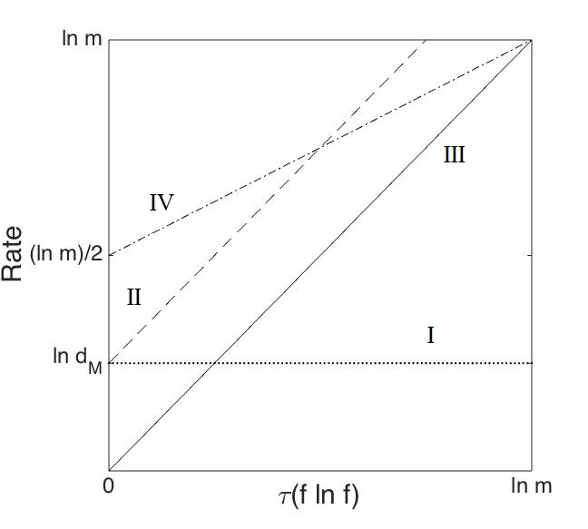
Figure 1. Combined bounds for quantum capacity of $\theta_{f}$ depending on $\tau(f\ln f)$. $\ln d_{M}$ varies from $0$ to $\frac{1}{2}\log m$. Curve I is $R=\ln d_{M}$. Curve II is $R=\ln d_{M}+\tau(f\ln f)$. Curve III is $R=\tau(f\ln f)$. Curve IV is $R=\frac{1}{2}(\ln m+\tau(f\ln f))$. The real values of $Q^{(1)}$ and $Q$ are in the quadrilateral surrounded by four lines. When $\ln d_{M}$ is small, our estimates are tight. This is the figure for $\ln d_{M}=\frac{1}{4}\ln m$.

8. Examples

8.1. Group channels

Starting from a finite group $G$, we will construct two classes of channels. We will use the quantum group framework [33] for both of these constructions. From a harmonic analysis point of view, group channels were also discussed in [11] for general locally compact groups. We restrict ourselves to finite groups here.

8.1.1. Hadamard channels

Generalized dephasing channels, as a special case of Hadamard channels, are called Schur multipliers in the operator algebra literature. The Hadamard channels are known to be degradable (see [16]), hence the quantum capacity does not require regularization, i.e. $Q^{(1)}=Q$. Our estimates overlap with the quantum capacity formula in [11] for finite groups, but both approaches are based on the unfortunately unpublished joint work [34]. The arguments, however, are different. Our approach provides a new proof of $Q=Q^{(p)}$ for these particular Schur multipliers, but this is already known thanks to the fact that Hadamard channels are strongly additive for $Q^{(1)}$ [62].

Suppose $G$ is a finite group with order $|G|=m$ and $1$ as its identity. We denote the group von Neumann algebra by $L(G)$, the algebra generated by $\{\lambda(g)|g\in G\}$ . Here $\lambda(g)$ is the left shift unitary defined on $B(l_{2}(G))$ as follows

$$\lambda(g)(e_{h})=e_{gh}\hskip 2.84544pt,\ \ \ \ \ \forall h\in G\hskip 2.84544pt,$$

where $\{e_{h}|h\in G\}$ is the canonical basis of $l_{2}(G)$, i.e. $e_{h}(g)=\delta_{h,g}$. The algebra of functions $l_{\infty}(G)$ is dual to $L(G)$ in sense of quantum groups and sits as diagonal matrices in $B(\ell_{2}(G))$. Let us denote by $e_{g,g}$ the diagonal matrix unit. Then $f=\sum_{g}f(g)e_{g,g}$ is in $l_{\infty}(G)$. The normalized traces on $L(G)$ and $l_{\infty}(G)$ are $\tau$ and $\tau^{\prime}$ respectively

$$\tau(\sum_{g}\alpha(g)\lambda(g))=\alpha(1),\ \ \tau^{\prime}(\sum_{g}f(g)e_{g,g})=\frac{1}{m}\sum_{g}f(g)\hskip 2.84544pt.$$

We note that $L_{2}(l_{\infty}(G),\tau^{\prime})\cong L_{2}(L(G),\tau)\cong l_{2}(G)$, and $l_{\infty}(G)\subset B(l_{2}(G))$, $L(G)\subset B(l_{2}(G))$ are both standard inclusions. The matrix Schur multiplication (or Hadamard product) is given by (here and in this section “$*$” always denotes the Schur multiplication for two matrices)

$$(a_{ij})*(b_{ij})=(a_{ij}\cdot b_{ij}).$$

It is a well-known fact (see [55]) that the multiplier map for a given matrix $a=(a_{ij})$,

$$M_{a}(b)=a*b\ \ \ \text{for}\ b=(b_{ij})\in M_{m}\hskip 2.84544pt,$$

is completely positive if and only if $a$ is positive. Moreover, $M_{a}$ is trace preserving if and only if $a_{ii}=1$ for $1\leq i\leq m$. In our situation, we further restrict the matrix $a$ to be a density in $L(G)$. The Stinespring unitary has the following form

$$U=\sum_{g}e_{g,g}\otimes\lambda(g)\in l_{\infty}(G)\otimes L(G)\hskip 2.84544pt.$$

This means $N=L(G)$ will be considered as the algebra of symbols, and $M=M^{\prime}=l_{\infty}(G)$. The VN-channel depending on a density $\rho=\sum\rho(g)\lambda(g)\in L(G)$ is defined as follows,

$$\theta_{\rho}(\omega) =id\otimes\tau[(\sum_{g}e_{g,g}\otimes\lambda(g)\omega\otimes\rho(\sum_{g}e_{g,g}\otimes\lambda(g)^{*})]$$

$$=\sum_{g,g^{\prime}}\tau(\lambda(g)\rho\lambda(g^{\prime})^{*})e_{g,g}\omega e_{g^{\prime},g^{\prime}}\hskip 2.84544pt=\hskip 2.84544pt(\rho(g^{-1}g^{\prime})){\rm*}(\omega_{g,g^{\prime}})\ \hskip 2.84544pt,$$

where $\omega=\sum_{g,g^{\prime}}\omega_{g,g^{\prime}}e_{g,g^{\prime}}\in S_{1}(l_{2}(G))$. This is a Schur multiplier by a density in $R(G)$. It is obvious that $|{e_{g,g}}\rangle$ and $|{\lambda(g)}\rangle$ are two orthogonal bases in $L_{2}(M)$ and $L_{2}(N)$ respectively. Hence Theorem 7.5 applies, we obtain

1. $-S_{cb}(\theta_{\rho})=Q^{(1)}(\theta_{\rho})=Q(\theta_{\rho})=Q^{(p)}(\theta_{\rho})=\tau(\rho\ln\rho)\hskip 2.84544pt,$

2. Since $\theta_{\rho}$ is unital, we have

   $$-S_{cb}(\theta_{\rho})+\ln m=C_{EA}(\theta_{\rho})=2Q_{EA}(\theta_{\rho})=\ln m+\tau(\rho\ln\rho)\hskip 2.84544pt,$$

   and these are attained at a maximally entangled state.

Note here $M=l_{\infty}(G)$ is commutitave, we have $\ln d_{l_{\infty}(G)}=0$. Thus in Figure.1 the Curve II and Curve III coincide and give the equality. In [11], the formula for $Q(\theta_{\rho})$ is obtained differently.

Example 8.1.

A well-studied qubit example is the dephasing channel. Let $0\leq q\leq 1$ be the dephasing parameter, we have

$$\Phi_{q}\large(\big{[}\begin{array}[]{cc}a&b\\ c&d\end{array}\big{]}\large)=\big{[}\begin{array}[]{cc}a&qb\\ qc&d\end{array}\big{]}\hskip 2.84544pt.$$

The channel can also be expressed using the Pauli matrix $Z=\left[\begin{array}[]{ccc}1&0\\ 0&-1\\ \end{array}\right]$,

$$\Phi_{q}(\rho)=(1-\frac{1-q}{2})\rho+\frac{1-q}{2}Z\rho Z\hskip 2.84544pt.$$

This corresponds to $G=\mathbb{Z}_{2}$ for $\rho=1+qX=\big{[}\begin{array}[]{cc}1&q\\ q&1\end{array}\big{]}$ in our setting. We obtain $Q(\theta_{\rho})=\tau(\rho\ln\rho)=\ln 2-H(\frac{1+q}{2})$, which is same with the formula in [60].

When the dimension $m>2$, we cannot recover an arbitrary generalized dephasing channels via the group construction, because the class of channels $\theta_{\rho}$ is a strict subset of all Schur multipliers.

8.1.2. Random unitary

A channel map is called a random unitary channel if it is a convex combination of unitary conjugation. Again, we use the shift unitaries $\{\lambda(g)\}$ defined above and $U=\sum_{g}e_{g,g}\otimes\lambda(g)$ as the Stinespring unitary defined as in the previous case. We switch, however, the roles of the environment and output. This means we consider $M^{\prime}=L(G)$ and the symbol algebra $N=l_{\infty}(G)$. Thus $M=R(G)$ as the right group von Neumann algebra generating by right shift unitary $\{r(g)|g\in G\}$. For each density $f\in l_{\infty}(G)$, we define the VN-channel by

$$\theta_{f}(\rho) =\tau^{\prime}\otimes id(U(f\otimes\rho)U^{*})=\sum_{g,g^{\prime}}\tau^{\prime}(e_{g,g}fe_{g^{\prime},g^{\prime}})\lambda(g)\rho\lambda(g^{\prime})^{*}$$

$$=\frac{1}{m}\sum_{g}f(g)\lambda(g)\rho\lambda(g)^{*}\ ,\ \ \ \forall\ \rho\in S_{1}(l_{2}(G))\hskip 2.84544pt.$$

Two extreme cases are $f=m\hskip 2.84544pte_{g,g}$ and $f=1$. The former one is a perfect unitary conjugation channel by $\lambda(g)$, and the latter one is the conditional expectation onto ${M=R(G)}$. Thanks to the Peter-Weyl theorem, here the index $d_{R(G)}$ is the largest degree of irreducible representations, or the dimension of the largest irreducible representations. For short, we denote $d_{G}\equiv d_{R(G)}$. Theorem 7.5 implies,

1. $\max\{\ln d_{G},\tau(f\ln f)\}\leq\!Q^{(1)}(\theta_{f})\!\leq\!Q(\theta_{f})\leq Q^{(p)}(\theta_{f})\!\leq\!\tau(f\ln f)+\ln d_{G};$

2. $-S_{cb}(\theta_{f})+\ln m=C_{EA}(\theta_{f})=2Q_{EA}(\theta_{f})=\ln m+\tau(f\ln f)$ is attained at a maximally entangled state.

Remark 8.2.

When the group $G$ is abelian, $R(G)$ is a commutative algebra. Then $d_{G}=0$, so upper and lower bounds coincide as the Hadamard channels:

$$-S_{cb}(\theta_{f})=Q^{(1)}(\theta_{f})=Q(\theta_{f})=Q^{(p)}(\theta_{f})=\tau(f\ln f)\hskip 2.84544pt.$$

In this case, we have $R(G)\cong l_{\infty}(\hat{G})$ with $\hat{G}$ being $G$’s dual group. For finite $G$, $G\cong\hat{G}$ so $\theta_{f}$ are also Hadamard channels.

Example 8.3.

The qubit example is the bit-flip channel. Let $G=\mathbb{Z}_{2}$, the nontrivial shift unitary is the pauli matrix $X=\left[\begin{array}[]{ccc}0&1\\ 1&0\\ \end{array}\right]$ . For the flip parameter $0\leq q\leq 1$ and qubit density $\rho\in S_{1}^{2}$,

$$\Phi_{q}(\rho)=(1-q)\hskip 2.84544pt\rho+q\hskip 2.84544ptX\rho X\hskip 2.84544pt.$$

One can see this is unitarily equivalent to the dephasing channel in Example 8.1 with dephasing parameter $\frac{1-q}{2}$.

In general the degree of the largest irreducible representation is not $1$, unless $G$ is commutative. There are several facts in representation theory giving upper bounds for the integer $d_{G}$. One we will use below is that if $H\subset G$ as an abelian subgroup, then $\max_{k}n_{k}\leq[G:H]$. We will compare the two upper bounds for $Q$ in the following examples.

Example 8.4.

For the dihedral groups $D_{2n}$, the group of symmetries of a $n$-regular polygon [19], our estimates are almost optimal. Indeed, for dihedral groups $d_{D_{2n}}$ is always $2$ for any $n\in{\mathbb{N}}$. So our estimates control everything up to one qubit

$$\max\{\ln 2,\tau(f\ln f)\}\leq Q^{(1)}(\theta_{f})\leq Q(\theta_{f})\leq Q^{(p)}(\theta_{f})\leq\tau(f\ln f)+\ln 2\hskip 2.84544pt.$$

When $n$ is large and $f$ is close to pure states, $\ln 2$ is small compared to $\tau(f\ln f)$ .

Example 8.5.

Let $G$ be the semi-product group $\mathbb{Z}_{d}^{l}\rtimes\mathbb{Z}_{l}$, where $\mathbb{Z}_{d}^{l}$ is the $l$ direct sum of cyclic groups $\mathbb{Z}_{d}$, $\mathbb{Z}_{l}$ does the shift action as follows,

$$(x_{1},x_{2},\cdots,x_{d},j)(x_{1}^{\prime},x_{2}^{\prime},\cdots,x_{l}^{\prime},j^{\prime})=( x_{1}+x_{1+j}^{\prime},x_{2}+x_{2+j}^{\prime},\cdots,x_{l}+x_{l+j}^{\prime},j+j^{\prime})\hskip 2.84544pt,$$

for any $1\leq x_{i},x^{\prime}_{i}\leq d,\ 0\leq i,j\leq l\hskip 2.84544pt.$ Note that since $\mathbb{Z}_{d}^{l}$ is an abelian subgroup of $G$, then it is easy to see that $d_{G}\leq l$. The comparison bound is better when $\tau(f\ln f)\leq l\ln d-2\ln l$. When $d$ is large, $\ln l\ll l\ln\sqrt{d}=|G|^{\frac{1}{2}}$.

Example 8.6.

For the symmetry group $|S_{n}|=n!$, it is shown in [56] that there exists constants $c_{1},c_{2}>0$ such that

$$-c_{1}\sqrt{n}\leq d_{S_{n}}-\frac{1}{2}\ln{n!}\leq-c_{2}\sqrt{n}\hskip 2.84544pt.$$

This implies that the comparison bound is better if $\tau(f\ln f)\leq 2c_{2}\sqrt{n}$ and the upper bound via $Q_{EA}$ bound is better when $\tau(f\ln f)\geq 2c_{1}\sqrt{n}$. Note although $[0,2c_{2}\sqrt{n}]$ is a relatively small region in the range of $\tau(f\ln f)$ (since $n\ll n!=|G|$), it is a definitely gaining part of the comparison estimate when the density $f$ is slightly perturbed from the identity $1$.

8.2. Pauli channels

Pauli channels are by no means optimal for the comparison bounds, but they do fit in our framework. Pauli channels are convex combinations of unitary conjugations by Pauli matrices. In high dimensions, we may interpret the Heisenberg-Weyl operators as the generalized Pauli matrices [59]. These operators are used to establish teleportation and superdense coding in high dimension. Let us consider $\{e_{k}|1\leq k\leq n\}$ as the standard basis of an $n$-dimensional complex Hilbert $H=l_{2}^{n}$. The generalized Pauli matrices $X$ and $Z$ for an $n$-dimensional system are

$$X(e_{k})=e_{k+1},\ \ Z(e_{k})=\exp({\frac{2k\pi i}{n}})e_{k}\ \ \text{for}\ \ 1\leq k\leq n\hskip 2.84544pt.$$

For $k=n$ we use the convention $e_{n+1}=e_{1}$. $X$ and $Z$ satisfy the commutation relations,

$$XZ=\exp({\frac{2k\pi i}{n}})ZX\hskip 2.84544pt.$$

Now an $n$-dimensional Pauli channel can be defined as follows,

$$\theta_{f}(\rho)=\frac{1}{n^{2}}\sum_{1\leq i,j\leq n}f_{ij}X^{i}Z^{j}\rho(X^{i}Z^{j})^{*}\hskip 2.84544pt.$$

In order to be a channel, the coefficient $f_{ij}$ must satisfy $f_{ij}\geq 0,\sum f_{ij}=n^{2}$. Now we consider $f\in N=l_{\infty}^{n^{2}}\subset B(l_{2}^{n^{2}})$, where $N$ is the commutative algebra spanned by ${\{P_{ij}|1\leq i,j\leq n\}}$ as its rank one projections. The normalized trace (which makes the operator $B$ a unitary) is given by $\tau(f)=\frac{1}{n^{2}}\sum_{ij}f(ij)$. We have the Stinespring dilation,

$$\theta_{f}(\rho)=\sum_{1\leq i,j\leq n}\tau(P_{ij}f)X^{i}Z^{j}\rho(X^{i}Z^{j})^{*}=id\otimes\tau(U(\rho\otimes f)U^{*})\hskip 2.84544pt,$$

where $U$ is a joint unitary in $B(l_{2}^{n})\otimes N$,

$$U=\sum_{1\leq i,j\leq n}X^{i}Z^{j}\otimes P_{ij}\hskip 2.84544pt.$$

One can easily see that $\theta_{f}$ is unital and $U$ satisfies the assumptions of Theorem 7.1. Indeed $\{X^{i}Z^{j}|1\leq i,j\leq n\}$ is an orthogonal basis for $M_{n}$ and $\{P_{ij}|1\leq i,j\leq n\}$ is an orthogonal basis for $L_{2}(\ell_{\infty}^{n^{2}}))$. Thus by Corollary 7.3 we deduce that

$$-S_{cb}(\theta_{f})=\tau(f\ln f)-\ln n,\ C_{EA}(\theta_{f})=2Q_{EA}(\theta_{f})=\tau(f\ln f)\hskip 2.84544pt.$$ (8.1)

For the comparison bound, we consider $\theta_{f}\otimes id_{M_{n}}$ instead of $\theta_{f}$. Note that ${\{X^{i}Z^{j}\otimes 1}_{i,j}$ is an orthogonal basis for $M_{n}\otimes 1$ and $M_{n}\otimes 1\subset M_{n}\otimes M_{n}$ is a standard inclusion as in the Example 6.1. This allows us to apply Theorem 3.1 and its corollary:

$$\ln n\leq Q^{(1)}(\theta_{f}\otimes id_{n})\leq Q(\theta_{f}\otimes id_{n})\leq Q^{(p)}(\theta_{f}\otimes id_{n})\leq\tau(f\ln f)+\ln n\hskip 2.84544pt.$$

Note that $Q^{(p)}$ is subadditive, we find

$$Q^{(p)}(\theta_{f}\otimes id_{n})=Q^{(p)}(\theta_{f})+\ln n\hskip 2.84544pt.$$

Hence

$$0\leq Q^{(1)}(\theta_{f})\leq Q(\theta_{f})\leq Q^{(p)}(\theta_{f})\leq\tau(f\ln f)\hskip 2.84544pt.$$

Thus for generalized Pauli channels, the comparison bound is always outperformed by (8.1) and entanglement assistance, i.e. $Q(\theta_{f})\leq Q_{EA}(\theta_{f})=\frac{1}{2}\tau(f\ln f)=\ln n-\frac{1}{2}H(\frac{1}{n^{2}}f)$ (because $\dim N=n^{2}$). This in the Figure.1 corresponds to the case $\ln d_{M}=\frac{1}{2}\ln m$, and hence the Curve IV is always lower then the Curve II. However, by applying an averaging trick, we obtain an new bound for potential quantum capacity $Q^{(p)}$ for high dimension depolarizing channel.

Example 8.7.

The $d$-dimensional depolarizing channel with parameter $q\in[0,1]$ is

$${\mathcal{D}}_{q}(\rho)\hskip 2.84544pt=\hskip 2.84544ptq\rho+(1-q)\frac{1}{d}\hskip 2.84544pt.$$

The depolarizing part $\rho\to\frac{1}{d}$ is actually the generalized Pauli channel with uniform distribution,

$$\frac{1}{d^{2}}\sum_{i,j}X^{i}Z^{j}\rho(X^{i}Z^{j})^{*}=tr(\rho)\frac{1}{d}.$$

Then ${\mathcal{D}}_{q}$ is the Pauli channel with the distribution $f_{00}=q+\frac{1-q}{d^{2}}$, $f_{ij}=\frac{1-q}{d^{2}}$ for $(i,j)\neq(0,0)$. Let us first consider the following dephasing channel

$$\Phi_{q^{\prime}}(\rho)=q^{\prime}\rho+(1-q^{\prime}){\mathcal{E}}(\rho)\hskip 2.84544pt,$$

where ${\mathcal{E}}$ is the conditional expectation onto the diagonal matrices (the completely dephasing channel) and $q^{\prime}\in[0,1]$. This channel dephases the off diagonal entry by a factor $q^{\prime}$ and by the discussion of 8.1.1 we know

$$Q^{(p)}(\Phi_{q}^{\prime})=\log d-\frac{(d-1)q^{\prime}+1}{d}\log\frac{(d-1)q^{\prime}+1}{d}-\frac{(d-1)(1-q^{\prime})}{d}\log\frac{(1-q^{\prime})}{d}\hskip 2.84544pt.$$

Similarly, the channel $\rho\to U^{*}\Phi_{q}^{\prime}(U\rho U^{*})U$ is also a dephasing channel but to the basis $\{Ue_{i}\}_{i}$ instead of the standard basis $\{e_{i}\}_{i}$. We claim that the averaging of dephasing channels uniformly on all basis will give us a depolaring channel. Namely for any state $\rho\in M_{d}$

$$\int_{U(M_{d})}U^{*}{\mathcal{E}}(U\rho U^{*})U=\frac{1}{d+1}\rho+\frac{1}{d+1}\hskip 2.84544pt.$$

This can be proved by the averaging the Choi matrix. Denote ${\mathcal{E}}_{U}=U^{*}{\mathcal{E}}(U\cdot U^{*})U$, let $\psi_{d}$ be the maximally entangled state $\sum_{i=1}^{d}e_{i}\otimes e_{i}$, then

$$\chi_{{\mathcal{E}}_{U}} =id\otimes{\mathcal{E}}_{U}(d|{\psi_{d}}\rangle\langle{\psi_{d}}|)=d\hskip 2.84544ptid\otimes U^{*}{\mathcal{E}}(1\otimes U|{\psi_{d}}\rangle\langle{\psi_{d}}|1\otimes U^{*})U$$

$$=did\otimes U^{*}{\mathcal{E}}(U^{t}\otimes 1|{\psi_{d}}\rangle\langle{\psi_{d}}|\bar{U}\otimes 1)U$$

$$=(U^{t}\otimes U^{*})id\otimes{\mathcal{E}}(d|{\psi_{d}}\rangle\langle{\psi_{d}}|)(\bar{U}\otimes U)$$

$$=(U^{t}\otimes U^{*})\chi_{{\mathcal{E}}}(\bar{U}\otimes U)$$

Note that $\chi_{\mathcal{E}}=\sum_{i=1}^{d}e_{i,i}\otimes e_{i,i}$ and hence the partial transpose on first component gives us

$$t\otimes 1((U^{t}\otimes U^{*})\chi_{{\mathcal{E}}}(\bar{U}\otimes U))=(U^{*}\otimes U^{*})\chi_{\mathcal{E}}(U\otimes U)\hskip 2.84544pt.$$

By representation theory ([10], Proposition $2.2$), we have

$$\int_{U(M)}\chi_{{\mathcal{E}}_{U}}=\frac{d}{d+1}|{\psi_{d}}\rangle\langle{\psi_{d}}|+\frac{1}{d+1}1\otimes 1\hskip 2.84544pt,$$

which proves the claim. Then for averaging the $q^{\prime}$-dephasing channel, we have

$$\int_{U(M_{d})}U^{*}\Phi_{q^{\prime}}(U\rho U^{*})U=(q^{\prime}+\frac{1-q^{\prime}}{d+1})\rho+\frac{1-q^{\prime}}{d+1}=D_{q^{\prime}+\frac{1-q^{\prime}}{d+1}}(\rho)\hskip 2.84544pt.$$

Set $q^{\prime}+\frac{1-q^{\prime}}{d+1}=q$, by convexity of $Q^{(p)}$ we get

$$Q^{(p)}({\mathcal{D}}_{q})\leq \log d-H(\frac{q(d^{2}-1)+1}{d^{2}})$$ (8.2)

$$-\frac{(d^{2}-1)(1-q)}{d^{2}}\log(d-1)\hskip 2.84544pt.$$

It is known that for $q\!\!\leq\!\!\frac{1}{d+1}$ the channel ${\mathcal{D}}_{p}$ becomes entanglement-breaking (it is an averaging of completely dephasing channel.) and hence $Q^{(p)}({\mathcal{D}}_{\frac{1}{d+1}})=0$ (see [62]). This upper bound (8.2) vanishes at $p=1/(d+1)$ and is convex in the interval $[1/(d+1),1]$. For $d=2$ it is [49] proved the upper bound

$$Q^{(p)}({\mathcal{D}}_{p})\leq 1-H(\frac{3p+1}{4})\hskip 2.84544pt,$$

by using a convex combination of dephasing channels to Pauli-$X,Y,Z$ basis. Using the unitaries from teleportation one can generalize their method to higher dimension, but that upper estimate only yields the first two terms in (8.2). Since the third term is negative, our upper bound are tighter for $d>2$.

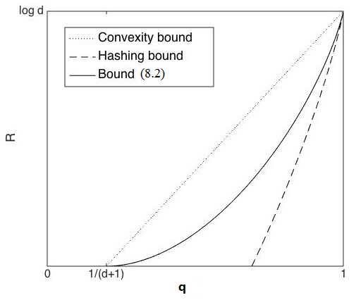
Figure 2. Our upper bound for the “one-shot” potential quantum capacity of a $d$-dimenional depolarizing channel: The dotted line is the convexity bound by the fact, $Q^{(p)}({\mathcal{D}}_{\frac{1}{d+1}})=0$. The dashed curve is the hashing (lower) bound. The solid curve is our new upper bound (8.2). This is the figure for $d=5$.

8.3. Majorana-Cliffords

The fourth class example we consider is Clifford algebra. The Clifford algebra $\mathit{Cl}_{n}$ has $n$ generators $\{C_{i}\}_{1\leq i\leq n}$, which satisfy the CAR (canonical anti-commutative relations):

$$C_{i}=C_{i}^{*}\ \ ,\ C_{i}C_{j}+C_{j}C_{i}=2\delta_{ij}\ \ \ \text{for}\ \ \forall 1\leq i,j\leq n\hskip 2.84544pt.$$

The self-adjoint property $C_{i}=C_{i}^{*}$ has a physical interpretation as creation and annihilation operators for Majorana fermions. Proposed candidates for Majorana fermions include supersymmetric analogs of bosons, dark matter, neutrinos, and electron-hole superpositions in topological condensed matter systems [58, 37]. Recent experiments have observed evidence of Majorana fermions in such condensed matter systems [42, 39, 9]. Condensed matter Majorana modes may serve as the basis for topological quantum computers [58], such as the physical motivation for the Drinfeld Double example below.

It is a known fact that $\mathit{Cl}_{n}$ is isomorphic to $2^{n}$-dimensional matrix algebra $M_{2^{n}}$. We have the canonical orthogonal basis of $L_{2}(\mathit{Cl}_{n},tr)$ defined by $\{C_{A}|A\subset[n]\}$, where $[n]=\{1,2,3\cdots,n\}$ and

$$C_{A}=\Pi_{i\in A}C_{i}:=C_{i_{1}}C_{i_{2}}\cdots C_{i_{k}}\hskip 2.84544pt\text{with}\hskip 2.84544pti_{1}<i_{2}<\cdots<i_{k}\ \ \text{and}\ \ \{i_{1},i_{2},\cdots,i_{k}\}=A\subset[n]\hskip 2.84544pt.$$

The order of the product matters because of the CAR. Similar to Pauli channels, let us set $N=l_{\infty}(2^{n})$ equipped with normalized trace $\tau$. The Stinespring unitary is

$$U=\sum_{A\subset[n]}C_{A}\otimes P_{A}\in M_{2^{n}}\otimes N\hskip 2.84544pt.$$

For a density (probability distribution) $f\in l_{\infty}(2^{n})$, we can define a Clifford channel

$$\theta_{f}(\rho)\hskip 2.84544pt=\hskip 2.84544ptid\otimes\tau(U(\rho\otimes f)U^{*})\hskip 2.84544pt=\hskip 2.84544pt\frac{1}{n^{2}}\sum_{A\subset[n]}f(A)C_{A}\rho{C_{A}}^{*}\hskip 2.84544pt,$$

as random unitaries. By Theorem 7.5, we obtain similar results as Pauli channels,

$$-S_{cb}(\theta_{f})=\tau(f\ln f)-n\ln 2\leq Q^{(1)}(\theta_{f}),\ C_{EA}(\theta_{f})=2Q_{EA}(\theta_{f})=\tau(f\ln f)\hskip 2.84544pt.$$ (8.3)

Again the upper bound via $Q_{EA}$ is tighter than the one given by the comparison theorem.

8.4. Quantum group channels

A finite dimensional quantum group is a Hopf algebra with an antipode. Quantum groups form a class of Hopf algebras that contains groups and their duals. More precisely, we are given a (finite dimensional) algebra $A$ and a $*$-homomorphism $\Delta:A\to A\otimes A$ and the co-multiplication which satisfies

$$(\Delta\otimes id_{A})\Delta\hskip 2.84544pt=\hskip 2.84544pt(id_{A}\otimes\Delta)\Delta\hskip 2.84544pt.$$

For locally compact quantum groups the antipode is determined by the left and right Haar weight (see [54]). Finite dimensional quantum groups are of Kac-type. For us this means that we have a trace $\tau$ such that

$$(\tau\otimes id)\Delta(x)\hskip 2.84544pt=\hskip 2.84544pt\tau(x)1\hskip 2.84544pt=\hskip 2.84544pt(id\otimes\tau)\Delta(x)\hskip 2.84544pt.$$

More importantly every quantum group (of Kac-type, see [3, 22]) admits a (multiplicative) unitary $V\in B(L_{2}(A))\otimes B(L_{2}(A))$ such that

$$\Delta(x)\hskip 2.84544pt=\hskip 2.84544ptV(x\otimes 1)V^{*}\hskip 2.84544pt.$$

Moreover, $V\in\hat{A}\otimes A$ (see [3] Section 3.6 and 3.8) with dual object $\hat{A}$. Following [33] we may define

$$\theta_{f}^{{\dagger}}(T)\hskip 2.84544pt=\hskip 2.84544ptid\otimes\tau((1\otimes f)V(T\otimes 1)V^{*})\hskip 2.84544pt,\hskip 2.84544pt\theta_{f}(\rho)\hskip 2.84544pt=\hskip 2.84544ptid\otimes\tau(V^{*}(\rho\otimes f)V)\hskip 2.84544pt.$$

Here $\theta_{f}^{{\dagger}}$ is the adjoint map of the channel $\theta_{f}$. Thus we find the Stinespring unitary $U=V^{*}\in\hat{A}\otimes A$ and $\Theta:L_{1}(A,\tau)\to CB(S_{1}(L_{2}(\hat{A}^{\prime}))$ the channel map. Here we may and will assume that $\tau$ is the restriction of the normalized trace on $B(L_{2}(A))$. Thus we set $N=A$ and $M=\hat{A}^{\prime}$, and they are of the same dimension. It was shown in the unpublished paper [34] that $B$ corresponds to the Fourier transform, and hence sends an orthonormal basis in $L_{2}(\hat{A}^{\prime})=L_{2}(\hat{A},\tau)$ to an orthonormal basis in $L_{2}(A,\tau)$. Therefore the assumptions of Theorem 7.5 are all satisfied and in particular,

$$Q^{(1)}(\theta_{f})\leq Q(\theta_{f})\leq Q^{(p)}(\theta_{f})\leq 2Q^{(1)}(\theta_{f})\hskip 2.84544pt.$$

Remark 8.8.

Here we have an trivial but interesting observation. Let $A$ be a finite dimensional quantum group with representation ${A=\oplus_{k}M_{n_{k}}}$. It is easy to see from representation theory $d_{A}\leq\sqrt{\dim A}$. On the other hand, we perform the construction above for $\hat{A}^{\prime}$ instead of $A$. Then $\theta_{1}$ is the conditional on $A$, and hence

$$\ln d_{A}\hskip 2.84544pt=\hskip 2.84544ptQ(\theta_{1})\leq\frac{1}{2}C_{EA}(\theta_{1})\hskip 2.84544pt=\hskip 2.84544pt\frac{\ln n+\tau(1\ln 1)}{2}=\frac{\ln n}{2}$$

where $n=\dim(A)=\dim(A^{\prime})$. This gives quantum information perspective of $d_{A}\leq\sqrt{\dim A}$.

8.5. Crossed product

Our particular Hadamard channels in 8.1.1 and random unitaries in 8.1.2 are quantum group channels for commutative or co-commutative symbol algebra. Here we will use crossed products to build a mixture of these two. A connection is found in Kitaev’s work on quantum computation by anyons [38]. Given a finite group $G$, we consider the operators $\{A_{g},B_{g}\hskip 2.84544pt|\hskip 2.84544ptg\in G\}$ satisfying the following relations

$$A_{h}A_{g}=A_{hg}\ ,\ B_{g}B_{h}=\delta_{g,h}B_{g}\ ,\ A_{g}B_{h}=B_{ghg^{-1}}A_{g}\hskip 2.84544pt,\hskip 2.84544pt\forall g,h\in G\hskip 2.84544pt.$$ (8.4)

They are the local gauge transformations and magnetic charge operators for vertices on a two-dimesional lattice in which edges correspond to spins. The crossed product corresponds to an algebra of local operators, which commute with the topological operators used to perform quantum computations. For this reason, the local operators generating the crossed product leave a significant subspace invariant, which in Kitaev’s physics corresponds to the space of degenerate ground states. This means that the anyonic quantum computer is naturally immune to local perturbations, possibly obviating the need for active error correction and presenting a quantum computation paradigm that resists decoherence due to its underlying physical structure.

Now consider $l_{\infty}(G)\subset B(l_{2}(G))$ as the diagonal matrices. Define the action $\alpha$ of $G$ acting on $l_{\infty}(G)$ as automorphism

$$\alpha_{g}(e_{h,h})=W_{g}e_{h,h}W_{g}^{*}=e_{ghg^{-1},ghg^{-1}}\hskip 2.84544pt,$$

where $W_{g}(e_{h})=e_{ghg^{-1}}$ are unitary in $B(l_{2}(G))$. The (reduced) crossed product $M=l_{\infty}(G)\rtimes_{\alpha}G$ is defined to be the algebra generated by the range of the following two representations on $l_{2}(G,l_{2}(G))\cong l_{2}(G)\otimes l_{2}(G)$,

$$\pi: l_{\infty}(G)\rightarrow B(l_{2}(G)\otimes l_{2}(G))\hskip 2.84544pt,\ \ \ \ \pi(x)=1\otimes x\ ;$$

$$\tilde{\lambda}: G\ \rightarrow B(l_{2}(G)\otimes l_{2}(G))\hskip 2.84544pt,\ \ \ \ \tilde{\lambda}(g)=\lambda(g)\otimes W_{g}\hskip 2.84544pt,$$

where $\lambda$ is the left regular representation of group $G$. We observe that $M,M^{\prime}\subset B(l_{2}(G\times G))$ is a standard inclusion, and the operator $J$ and commutant $M^{\prime}$ are given as follows,

$$J(e_{g}\otimes e_{h})=e_{g^{-1}}\otimes e_{g^{-1}hg}\hskip 2.84544pt,\hskip 2.84544ptJ\pi(x)J=\sum_{g}e_{g,g}\otimes W_{g}xW_{g}^{*}\ ,\ \ J\tilde{\lambda}(g)J=r(g)\otimes 1\hskip 2.84544pt.$$

Thus neither $M$ nor $M^{\prime}$ is commutative. Denote $A_{g}=\lambda(g)\otimes W_{g}$ and $B_{h}=1\otimes e_{h,h}$, one can check they satisfy the commutation relations (8.4) in Kitaev’s setting. Now we are ready to use these operators to construct channels.
Case 1. Consider the Stinespring unitary $U\in M^{\prime}\otimes B(l_{2}(G\times G))$

$$U=\sum_{g,h}(A_{g}B_{h})\otimes(\lambda(h)\otimes e_{g,g})\hskip 2.84544pt,$$

with the first bracket elements in $M$ and second bracket in $N=L(G)\bar{\otimes}l_{\infty}(G)$. For $f\in L(G)\otimes l_{\infty}(G)$, we can write $f=\sum_{g}f_{g}\otimes e_{g,g}$, where each $f_{g}=\sum_{h}f_{g}(h)\lambda(h)\in L(G)$. The channel for a density $f\in N$ is defined as follows,

$$\theta_{f}:S_{1}(l_{2}(G\times G))\rightarrow S_{1}(l_{2}(G\times G))$$

$$\theta_{f}(\rho)=\sum_{g,g^{\prime},h,h^{\prime}}\tau[(\lambda(h)\otimes e_{g,g})f(\lambda(h^{\prime})^{*}\otimes e_{g^{\prime},g^{\prime}})]A_{g}B_{h}\rho(A_{g^{\prime}}B_{h^{\prime}})^{*}$$

$$=\sum_{g,h,h^{\prime}}f_{g}(h^{\prime-1}h)\lambda(g)\rho_{h,h^{\prime}}\lambda(g)^{*}\otimes e_{ghg^{-1},gh^{\prime}g^{-1}},\ \ \forall\hskip 2.84544pt\rho=\sum_{g,h\in G}\rho_{h,h^{\prime}}\otimes e_{h,h^{\prime}}\in S_{1}(l_{2}(G\times G))\hskip 2.84544pt.$$

One can see that this channel is a mixture of random unitary and Schur multiplier. It is unital because

$$\theta_{f}(1)=\sum_{g,h}\tau(f_{g})1_{B(l_{2}(G))}\otimes e_{ghg^{-1},ghg^{-1}}=1_{B(l_{2}(G)\otimes l_{2}(G))}\hskip 2.84544pt.$$

It is easy to check that $U$ satisfies assumptions of Theorem 7.5. Note that $dimM=n^{2}$, we have

1. $-S_{cb}(\theta_{f})=\tau(f\ln f),\ C_{EA}(\theta_{f})=2Q_{EA}(\theta_{f})=\tau(f\ln f)+2\ln n$;

2. $\max\{d_{M},\tau(f\ln f)\}\leq Q^{(1)}(\theta_{f})\leq Q(\theta_{f})\leq Q^{(p)}(\theta_{f})=\tau(f\ln f)+\max_{k}\ln n_{k}\hskip 2.84544pt.$

Case 2. Consider another unitary

$$U^{\prime}=\sum_{g,h}(A_{g}B_{h})\otimes e_{hg,g}\hskip 2.84544pt.$$

Now the symbol algebra $N$ is $B(l_{2}(G))$. For a density, $f=\sum_{g,h}f_{g,g^{\prime}}e_{g,g^{\prime}}\in N$, we define the channel $\theta_{f}:S_{1}(l_{2}(G\times G))\to S_{1}(l_{2}(G\times G))$ associated with $f$ as

$$\theta_{f}(\rho)=\sum_{g,g^{\prime},h,h}\tau(e_{hg,g}fe_{g^{\prime},h^{\prime}g^{\prime}})A_{g}B_{h}\rho(A_{g}B_{h})^{*}=\frac{1}{n}\sum_{hg=h^{\prime}g^{\prime}}f_{g,g^{\prime}}(\lambda(g)\rho_{h,h^{\prime}}\lambda(g)^{*}\otimes W_{g}e_{h,h^{\prime}}W_{g^{\prime}}^{*}),$$

for any $\rho=\sum_{h,h^{\prime}\in G}\rho_{h,h^{\prime}}\otimes e_{h,h^{\prime}}\in S_{1}(l_{2}(G\times G))\hskip 2.84544pt.$ Again it is unital, so our theorem give the same estimates as case 1.

8.6. Non-unital channels

So far the examples above are unital channels. In this part, we provide a non-unital example for which our estimates still apply. Let $G$ be a finite group of order $m$, and $g,h\in G$ be its group elements. Denote $B(l_{2}(G))\cong M_{m}$ and $e_{g,h}$ as the matrix units. Consider the Stinespring unitary

$$U=\sum_{g,h\in G}e_{gh,h}\otimes e_{g,gh}\in M_{m}\otimes M_{m}\hskip 2.84544pt.$$

For each density $f\in(M_{m},\frac{1}{m}tr)$ (for the symbol algebra we use the normalized trace), we may define $\theta_{f}:S_{1}^{m}\rightarrow S_{1}^{m}$ as follows

$$\theta_{f}(\rho) =\frac{1}{m}\sum_{g,h,h^{\prime}\in G}f_{gh,gh^{\prime}}\rho_{h,h^{\prime}}e_{gh,gh^{\prime}}=\frac{1}{m}\sum_{g}f*(\lambda(g)\rho\lambda(g)^{*})$$

$$=f*(\frac{1}{m}\sum_{g}\lambda(g)\rho\lambda(g)^{*})\hskip 2.84544pt,\ \ \ \ \ \forall\rho=\sum_{h,h^{\prime}}\rho_{h,h^{\prime}}e_{h,h^{\prime}}\in S_{1}(l_{2}(G))\hskip 2.84544pt.$$

Here “$*$” is again the Schur multiplication and $\lambda$ is the left regular representation. One can see that this channel is a composition of a random unitary and a Schur multiplier. In general this channel is not unital,

$$\theta_{f}(1)=\frac{1}{m}\sum_{g}f*1={\mathcal{E}}(f)\hskip 2.84544pt.$$

Here ${\mathcal{E}}$ denote the conditional expectation onto the diagonal matrices $f=\sum_{g}f_{g,g}e_{g,g}$. Since $\{e_{gh,h}\}$ and $\{e_{g,gh}\}$ are orthogonal basis of the full matrix algebra $M_{m}$, Theorem 7.5 implies

$$-S_{cb}(\theta_{f})=\tau(f\ln f)-\ln m,\ \ \ \ C_{EA}(\theta_{f})=2Q_{EA}(\theta_{f})\leq\tau(f\ln f)\hskip 2.84544pt,$$

$$H(\frac{1}{m}{\mathcal{E}}(f))-H(\frac{1}{m}f)\leq Q^{(1)}(\theta_{f})\leq Q(\theta_{f})\leq\frac{1}{2}\tau(f\ln f)\hskip 2.84544pt.$$ (8.5)

In particularly, we know $H(\frac{1}{m}{\mathcal{E}}(f))-H(\frac{1}{m}f)\geq 0$, because unital channels always increase the entropy. As for Pauli channels, the comparison estimates apply for $id\otimes\theta_{f}$ instead of $\theta_{f}$, but (8.6) is tighter than the comparison estimates.

Acknowledgement—We thank Mark M. Wilde for helpful discussion and passing along the reference [12], Andreas Winter and Debbie Leung for interesting remarks on the potential quantum capacity, and Carlos Palazuelos for continuing discussions on capacities. MJ is partially supported by NSF-DMS 1501103. NL is supported by NSF Graduate Research Fellowship Program DGE-1144245.

References

- 1. Abeyesinghe, A., Devetak, I., Hayden, P., Winter, A.: The mother of all protocols: Restructuring quantum information s family tree. Proc. Roy. Soc. London Ser. A, rspa20090202 (2009)
- 2. Aubrun, G., Szarek, S., Werner, E.: Hastings’s additivity counterexample via dvoretzky’s theorem. Comm. Math. Phys. 305, 85–97 (2011)
- 3. Baaj, S., Skandalis, G.: Unitaires multiplicatifs et dualité pour les produits croisés de mathrm -algèbres. Ann. Sci. École Norm. Sup., 26, 425–488 (1993)
- 4. Bell, J.S.: On the Einstein-Podolsky-Rosen paradox. Physics 1, 195–200 (1964)
- 5. Bennett, C.H., DiVincenzo, D.P., Smolin, J.A.: Capacities of quantum erasure channels. Phys. Rev. Lett. 78, 3217 C3220 (1997)
- 6. Bennett, C.H., Shor, P.W., Smolin, J., Thapliyal, A.V.: Entanglement-assisted capacity of a quantum channel and the reverse shannon theorem. IEEE Trans. Inform. Theory 48, 2637–2655 (2002)
- 7. Bergh, J., Löfström, J.: Interpolation spaces. An introduction. Berlin: Springer, 1976
- 8. Blecher, D.P., Paulsen, V.I.: Tensor products of operator spaces. J. Funct. Anal. 99, 262–292 (1991)
- 9. Bunkov, Y., Gazizulin, R.: Majorana fermions: Direct observation in 3He. arXiv:1504.01711
- 10. Collins, B., Śniady, P.: Integration with respect to the Haar measure on unitary, orthogonal and symplectic group. Comm. Math. Phys. 264, 773-795 (2006)
- 11. Crann, J., Neufang, M.: Quantum channels arising from abstract harmonic analysis. J. Phys. A 46 045308 (2013)
- 12. Cubitt, T., Elkouss, D., Matthews, W., Ozols, M., Pérez-Garcia, D., Strelchuk, S.: Unbounded number of channel uses may be required to detect quantum capacity. Nat. Commun. 6 (2015)
- 13. Devetak, I.: The private classical capacity and quantum capacity of a quantum channel. IEEE Trans. Inform. Theory 51, 44–55 (2005)
- 14. Devetak, I., Harrow, A.W., Winter, A.: A family of quantum protocols. Phys. Rev. Lett. 93, 230504 (2004)
- 15. Devetak, I., Junge, M., King, C., Ruskai, M.B.: Multiplicativity of completely bounded -norms implies a new additivity result. Comm. Math. Phys. 266, 37–63 (2006).
- 16. Devetak, I., Shor, P.W.: The capacity of a quantum channel for simultaneous transmission of classical and quantum information. Comm. Math. Phys. 256, 287 C303 (2005)
- 17. DiVincenzo, D.P., Shor, P.W., Smolin, J.A.: Quantum-channel capacity of very noisy channels. Phys. Rev. A 57, 830 (1998)
- 18. Drinfeld, V.G.: Quantum groups Zapiski Nauchnykh Seminarov POMI 155, 18-49 (1986)
- 19. Dummit, D., Foote, R.M.: Abstract algebra. Hoboken: Wiley, 2004
- 20. Effros, E., Ruan, Z.: Operator spaces. New York: Oxford University Press, 2000
- 21. Einstein, A., Podolsky, B., Rosen, N.: Can quantum-mechanical description of physical reality be considered complete? Physical Review 47, 777 C780 (1935)
- 22. Enock, M., Schwartz, J.M.: Kac algebras and duality of locally compact groups. Berlin: Springer Science & Business Media, 2013
- 23. Fuglede, B., Kadison, R.V.: Determinant theory in finite factors. Ann. of Math. 520–530 (1952)
- 24. Fukuda, M., Wolf, M.M.,: Simplifying additivity problems using direct sum constructions. J. Math. Phys. 48, 072101 (2007)
- 25. Garcia-Patrón, R., Pirandola, S., Lloyd, S., Shapiro, J.H.: Reverse coherent information. Phys. Rev. Lett. 102, 210501 (2009)
- 26. Giovannetti, V., Fazio, R.: Information-capacity description of spin-chain correlations. Phys. Rev. A 71, 032314 (2005)
- 27. Gupta, M.K., Wilde, M.M.: Multiplicativity of completely bounded -norms implies a strong converse for entanglement-assisted capacity. Comm. Math. Phys. 334, 867–887 (2015)
- 28. Haagerup, U.: The standard form of von neumann algebras. Mathematica Scandinavica 37, 271–283 (1975)
- 29. Haagerup, U., Musat, M.: Factorization and dilation problems for completely positive maps on von neumann algebras. Comm. Math. Phys. 303, 555–594 (2011)
- 30. Hayden, P., Winter, A.: Counterexamples to the maximal p-norm multiplicativity conjecture for all . Comm. Math. Phys. 284, 263–280 (2008)
- 31. Holevo, A.S.: The capacity of the quantum channel with general signal states. IEEE Trans. Inform. Theory 44, 269-273 (1998)
- 32. Holevo, A.S., Werner, R,F,: Evaluating capacities of bosonic Gaussian channels. Phys. Rev. A 63, 032312 (2001)
- 33. Junge, M., Neufang, M., Ruan, Z.: A representation theorem for locally compact quantum groups. Int. J. Math. 20, 377–400 (2009)
- 34. Junge, M., Neufang, M., Ruan, Z.: Reversed coherent information for quantum group channels. Private communication (2009)
- 35. Junge, M., Palazuelos, C.: Cb-norm estimates for maps between noncommutative -spaces and quantum channel theory. Internat. Math. Res. Notices, rnv161 (2015)
- 36. Junge, M., Palazuelos, C.: Channel capacities via p-summing norms. Adv. Math. 272, 350–398 (2015)
- 37. Kitaev, A.Y.: Unpaired majorana fermions in quantum wires. Physics-Uspekhi 44, 131 (2001)
- 38. Kitaev, A.Y.: Fault-tolerant quantum computation by anyons. Ann. Physics 303, 2–30 (2003)
- 39. Li, J., Chen, H., Drozdov, I.K., Yazdani, A., Bernevig, B.A., MacDonald, A.H.: Topological superconductivity induced by ferromagnetic metal chains. Phys. Rev. B 90, 235433 (2014)
- 40. Lloyd, S.: Capacity of the noisy quantum channel. Phys. Rev. A 55, 1613 (1997)
- 41. Müller-Lennert, M., Dupuis, F., Szehr, O., Fehr, S., Tomamichel, M.: On quantum Rényi entropies: A new generalization and some properties. J. Math. Phys. 54, 122203 (2013)
- 42. Nadj-Perge, S., Drozdov, I., Li, J., et al: Observation of majorana fermions in ferromagnetic atomic chains on a superconductor. Science 346, 602-607 (2014).
- 43. Nakamura, M., Umegaki, H.: A note on the entropy for operator algebras. Proceedings of the Japan Academy 37, 149–154 (1961)
- 44. Pisier, G.: Noncommutative vector valued -spaces and completely -summing maps. Asté risque 247, 1-131 (1993)
- 45. Pisier, G.: Introduction to operator space theory. Cambridge University Press, 2003
- 46. Schumacher, B., Westmoreland, M.D.: Sending classical information via noisy quantum channels. Phys. Rev. A 56, 131 (1997)
- 47. Shannon, C.E.: A mathematical theory of communication. Bell System Technical Journal 27,379 C423 (1948)
- 48. Shor, P.W.: The quantum channel capacity and coherent information. In lecture notes, MSRI Workshop on Quantum Computation. 2002
- 49. Smith, G., Smolin, J., Winter, A.: The quantum capacity with symmetric side channels. IEEE Trans. Inform. Theory 54, 4208–4217 (2008)
- 50. Smith, G., Smolin, J.A.: Degenerate quantum codes for Pauli channels. Phys. Rev. Lett. 98, 030501 (2007)
- 51. Sutter, D., Scholz, V.B., Renner, R.: Approximate degradable quantum channels. 2015 IEEE International Symposium on Information Theory (ISIT) 2767–2771 (2015)
- 52. Tomamichel, M., Wilde, M.M., Winter, A.: Strong converse rates for quantum communication. 2015 IEEE International Symposium on Information Theory (ISIT), 2386–2390 (2015)
- 53. Takesaki, M.: Theory of operator algebras II. Springer Science & Business Media, 2013
- 54. Vaes, S., Vergnioux, R.: The boundary of universal discrete quantum groups, exactness, and factoriality. Duke Math. J. 140, 35–84 (2007)
- 55. Vern, P.: Completely bounded maps and operator algebras. Cambridge University Press, 2003.
- 56. Vershik, A.M., Kerov, S.V.: Asymptotic of the largest and the typical dimensions of irreducible representations of a symmetric group. Funct. Anal. Appl. 19, 21–31 (1985)
- 57. Wang, X., Duan, R.: A semidefinite programming upper bound of quantum capacity. arXiv:1601.06888
- 58. Wilczek, F.: Majorana returns. Nat. Phys. 5, 614–618 (2009)
- 59. Wilde, M.M.: Quantum information theory. Cambridge University Press, 2013.
- 60. Wilde, M.M., Hsieh, M.: The quantum dynamic capacity formula of a quantum channel. Quantum Information Process 11, 1431–1463 (2012)
- 61. Wilde, M.M., Winter, A., Yang, D.: Strong converse for the classical capacity of entanglement-breaking and Hadamard channels via a sandwiched Renyi relative entropy. Comm. Math. Phys. 331, 593–622 (2014)
- 62. Yang, D., Winter, A.: Potential capacities of quantum channels (2015). IEEE Trans. Inform. Theory 62, 1415–1424 (2016)