Anderson localization of light in disordered superlattices containing graphene layers

Abstract

We theoretically investigate light propagation and Anderson localization in one-dimensional disordered superlattices composed of dielectric stacks with graphene sheets in between. Disorder is introduced either on graphene material parameters (e.g. Fermi energy) or on the widths of the dielectric stacks. We derive an analytic expression for the localization length $\xi$, and compare it to numerical simulations using transfer matrix technique; a very good agreement is found. We demonstrate that the presence of graphene may strongly attenuate the anomalously delocalised Breswter modes, and is at the origin of a periodic dependence of $\xi$ on frequency, in contrast to the usual asymptotic decay, $\xi\propto\omega^{-2}$. By unveiling the effects of graphene on Anderson localization of light, we pave the way for new applications of graphene-based, disordered photonic devices in the THz spectral range.

I Introduction

Due to its extraordinary electronic and optical properties, graphene has emerged as an alternative material platform for applications in photonics and optoelectronics Avouris and Freitag (2014); Bludov et al. (2013a); Zhan et al. (2013). A partial but by no means exhaustive list of applications of graphene in photonics include high-speed photodetectors Xia et al. (2009), optical modulators Liu et al. (2011), plasmonic devices Garcia de Abajo (2014); Ju et al. (2011); Echtermeyer et al. (2011), and ultrafast lasers Sun et al. (2010). In addition, graphene is a promising candidate to overcome one of the major existing hurdles to bring optics and electronics together, namely the efficient conversion between optical and electronic signals. Indeed, this can be facilitated by the fact that graphene enables strong, electric field-tunable optical transitions, and resonantly enhances light-mater interactions in sub-wavelength volumes. In practice this can be achieved, for instance, by integrating a graphene layer into a photonic crystal nanocavity Engel et al. (2012). The presence of graphene also allows for an efficient electro-optical modulation of photonic crystals nanocavities by electrostatic gating Majumdar et al. (2013); Gan et al. (2013). However, the integration of graphene into photonic crystals is naturally prone to unavoidable disorder associated to the fabrication process. This constitutes per se a motivation to investigate the effects of disorder in photonic crystals containing graphene layers which, as far as we know, have not been considered in the literature so far. In addition to this technological and practical motivation, there is a very fundamental one as well, namely to understand the impact of graphene on Anderson localization of light.

The concept of Anderson localization (AL) was originally conceived in the realm of condensed matter physics as a disorder driven metal-insulator transition Anderson (1958). Being an interference wave phenomenon, this concept has been extended to light Segev et al. (2013), acoustic waves Hu et al. (2008), and even Bose-Einstein condensed matter waves Billy et al. (2008). As a result, Anderson localization is today a truly interdisciplinary topic, and important contributions have emerged from different areas, ranging from condensed matter, photonics, acoustics, atomic physics, and seismology Lagendijk et al. (2009). Dimensionality is crucial to AL, and in 1D the vast majority of states is exponentially localised on a length scale given by the localization length $\xi$, regardless of the disorder strength. In optical systems exceptions do exist, and delocalised modes may occur in low-dimensional systems as a result of the presence of correlations Izrailev et al. (2012), necklace modes Bertolotti et al. (2005), or metamaterials with negative refraction Mogilevtsev et al. (2010, 2011); Asatryan et al. (2007). The question of whether these anomalies occur when graphene is integrated into disordered optical superlattices remains an open question.

Bearing in mind both these technological and fundamental motivations, in the present paper we undertake an analytical and numerical investigation of Anderson localization of light in one-dimensional disordered superlattices composed of dielectric stacks with graphene layers in between, as depicted in Fig. 1. We consider two possible, realistic ways to model disorder: compositional and structural disorder. In the former case disorder is introduced in graphene’s material parameters, such as the Fermi energy, whereas in the latter the dielectric components of the superlattice have random widths. In both cases, we derive an analytic expression for the localization length $\xi$, and compare it to numerical simulations using a transfer matrix technique; an overall very good agreement is found. In the case where the medium impedances match, we find that $\xi$ exhibits an oscillatory behaviour as a function of frequency $\omega$, in contrast to the usual asymptotic decay $\xi\propto\omega^{-2}$. We demonstrate that graphene may strongly suppress the anomalously delocalised Brewster modes, as it induces additional reflexions at the superlattice interfaces. We also investigate the effects of inter and intraband transitions of the graphene conductivity on $\xi$, identifying the regimes where Anderson localization and absorption dominates light transmission.

This paper is organised as follows. In Sec. II we present the analytical results, where we derive an expression for the localization length of disordered superlattices containing graphene sheets. In Sec. III we present and discuss the numerical simulations, based on transfer matrix technique, which are also compared to the analytical calculations. Finally, Sec. IV is devoted to the concluding remarks. We also present a number of appendices giving the details of the calculations and aiming at making the the text as self-contained as possible. To our best knowledge, there are only two published papersKuzmiak and Maradudin (1997); Soto-Puebla et al. (2004) dealing with similar problems to the one we consider in this paper, but in the context a metals, in which case only Drude’s conductivity plays a role.

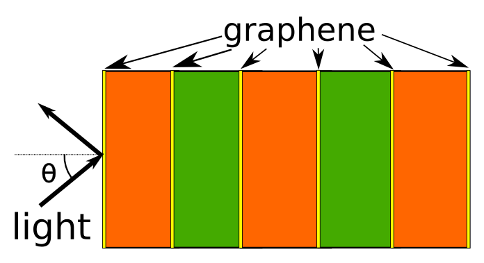
Figure 1: Color on-line. Schematic representation of the system.

II Analytical calculation of the localization length

Light propagation in a 1D superlattice containing graphene layers (Fig. 1) is modelled by the transfer matrix formalism Markos and Soukoulis (2008). The $M^{n}=\{m^{n}_{ij}\}$ transfer matrix connects the fields at the right of the $n-$th unit cell to those at left according to:

$$\psi^{n+1}=M^{n}\psi^{n},$$ (1)

where $\psi^{n}=\begin{bmatrix}\psi_{R}^{n}&&\psi_{L}^{n}\end{bmatrix}^{T}$, and $\psi_{R}^{n}$ ($\psi_{L}^{n}$) refers to the right (left) propagating field in the $n-$th cell. For transverse electric (TE) and transvere magnetic (TM) modes, $\psi$ refers to the electric and magnetic field, respectively. We consider the particular case where $\det M^{n}=1$, which occurs for systems with preserved time reversal symmetry Markos and Soukoulis (2008). In this case, one can show that $M^{n}$ may be written as

$$M^{n}=\begin{pmatrix}\cosh\phi_{1}^{n}e^{i\phi_{2}^{n}}&&\sinh\phi_{1}^{n}e^{i\phi_{3}^{n}}\\ \sinh\phi_{1}^{n}e^{-i\phi_{3}^{n}}&&\cosh\phi_{1}^{n}e^{-i\phi_{2}^{n}}\end{pmatrix},$$ (2)

where $\phi_{i}^{n}$ are parameters that depend on the composition of the $n-$th cell. (from here on we omit the $n$ dependence in $\phi_{i}$, except when strictly necessary to avoid any confusion.) For periodic systems with preserved time-reversed symmetry, $\phi_{i}$ are real numbers and all the $M^{n}$’s are equal. We thus write $M^{n}=M^{0}$. One can write the photonic dispersion relation Markos and Soukoulis (2008) as $\cos\gamma=(m_{11}^{0}+m_{22}^{0})/2$, where

$$\cos\gamma=\cosh\phi_{1}^{0}\cos\phi_{2}^{0}\,.$$ (3)

Disorder is introduced in the parameters $\phi_{i}$:

$$\phi_{i}=\phi^{0}_{i}+\delta\phi_{i}\,$$ (4)

where $\delta\phi_{i}$ describes random fluctuations around the average value, and which may have different origins, as it will be detailed later in the paper. For a periodic system, a transformation $M_{\text{transf}}=M_{\text{circle}}M_{\text{real}}$ (see appendix A) exists that maps the variables $\psi^{n}_{R,L}$ into a new set of variables, denoted by $Q_{n}$ and $P_{n}$, such that $X^{T}=[Q^{n}\,\,P^{n}]^{T}=M_{\text{transf}}[\psi^{n}_{R}\,\,\psi^{n}_{L}]^{T}$. These new variables describe a circle in phase space Izrailev and Makarov (2009), with radius $\sqrt{Q_{n}^{2}+P_{n}^{2}}$ proportional to the electric field amplitude. Applying this transformation to Eq. (1), the transformed matrix $M^{\prime}=M_{\text{transf}}M^{n}M_{\text{transf}}^{-1}$ reads

$$M^{\prime}=\begin{pmatrix}E_{n}&&F_{n}\\ G_{n}&&H_{n}\end{pmatrix},$$ (5)

where:

$$E_{n} = \cosh\phi_{1}\cos\phi_{2}-\sinh\phi_{1}\sin\delta\phi_{3},$$ (6)

$$F_{n} = -v^{2}\left(\cosh\phi_{1}\sin\phi_{2}+\sinh\phi_{1}\cos\delta\phi_{3}\right),$$ (7)

$$G_{n} = v^{-2}\left(\cosh\phi_{1}\sin\phi_{2}-\sinh\phi_{1}\cos\delta\phi_{3}\right),$$ (8)

$$H_{n} = \cosh\phi_{1}\cos\phi_{2}+\sinh\phi_{1}\sin\delta\phi_{3}.$$ (9)

with $v$ and $\tau$ defined in appendix A. When $\phi_{i}=\phi_{i}^{0}$, we have $\delta\phi_{3}=0$ and Eqs. (6)-(9) lead to $E_{n}=H_{n}=\cos\gamma$ and $F_{n}=-G_{n}=\sin\gamma$. When weak disorder is introduced, the trajectory of the points $(Q_{n},P_{n})$ results in a perturbation of the circle. The recurrence equations defined by $X^{n+1}=M^{\prime}X^{n}$ are similar to a Hamiltonian map of the classical harmonic oscillator subjected to a parametric impulsive forceIzrailev et al. (1995), where $Q_{n}$ and $P_{n}$ are the coordinate and conjugated moments, respectively, and $\gamma$ is the phase between successive kicks.

The presence of disorder introduces a key length scale, the localization length $\xi$. In 1D electronic systems all eigenmodes are exponentially localised, although some exceptions do exist in the realm of optical systems Mogilevtsev et al. (2010, 2011); Asatryan et al. (2007); Bertolotti et al. (2005) (see Introduction). The length $\xi$ characterises the exponential decay of the eigenfunctions and is defined in terms of the reciprocal of the Lyapunov exponent $\lambda$. In 1D $\lambda$ can be written as Markos and Soukoulis (2008); Izrailev and Makarov (2009):

$$\lambda=\frac{1}{2}\left\langle\ln\left|\frac{\psi^{n+1}_{R}}{\psi^{n}_{R}}\right|^{2}\right\rangle\,.$$ (10)

In Eq. (10) the brackets denote averaging over both ensembles and the system unit cells, while the usual definition of the localization length considers only averages over ensembles Markos and Soukoulis (2008). The two definitions are equivalent. The relation between $\lambda$ and $\xi$ is:

$$\text{Re}\lambda=\frac{d}{\xi},$$ (11)

where $d$ is the mean length of the unit cell. The advantage of the approach based on the parameters $P_{n}$ and $Q_{n}$ is that we can use polar (or action-angles) coordinates:

$$P_{n}=R_{n}\sin\Theta_{n},$$

$$Q_{n}=R_{n}\cos\Theta_{n}\,.$$ (12)

Without disorder, $R_{n}$ is a constant and $\Theta_{n}$ increases by minus the Bloch phase, $-\gamma$, as we move from unit cell to unit cell. With disorder, the radius $R_{n}$ changes in every step, with $R_{n+1}$ a function of $R_{n}$, $\Theta_{n}$, and of the matrix elements of $M^{n}$. The angle $\Theta_{n+1}$ only depends on $\Theta_{n}$ and $M^{n}$. For weak disorder a recurrence equation (47) exists that, in the continuum limit, becomes a stochastic Îto equation which has a corresponding Fokker-Planck equation Izrailev et al. (1998) . In this case, the first approximation for the density probability function of $\Theta_{n}$ is uniform in the interval $[0,2\pi]$ for $\gamma\neq 0,\pi/2,\pi$.

Writing Eq. (10) in terms of $R$ and $\Theta$, and averaging over $\Theta$ with uniform density probability, we obtain, up to second order in $\delta\phi_{i}$:

$$\lambda=\frac{1}{2}\left\langle Y_{1}+Y_{2}\cos 2\Theta_{n}+Y_{3}\sin 2\Theta_{n}-\frac{1}{4}Y_{2}^{2}-\frac{1}{4}Y_{3}^{2}\right\rangle,$$ (13)

where $Y_{i}$, with $i=1,2,3$ are defined in Appendix B and depend on the matrix elements $M^{n}$.

In the following sections we will study the propagation of light through a disordered structure of alternating graphene sheets and dielectric layers. In this case each propagation matrix $M^{n}$ is determined by the widths $z_{i}$, the incidence angle $\theta_{i}$, the dielectric material parameters $\mu_{i}$ and $\varepsilon_{i}$, and the graphene conductivity $\sigma$. In the present work we focus on the cases where disorder is present in the widths of the stacks (structural disorder) and on graphene conductivities (compositional disorder) . Both are realistic situations that may occur in the fabrication of these structures.

For the type of structural disorder studied here the width of each layer $i$ of the $n^{\rm{th.}}$ cell is a random variable

$$z_{i}(n)=z_{i}^{0}+\zeta_{i}(n),$$ (14)

where $\zeta_{i}$ are uncorrelated random variables with zero mean and mean standard deviation $\sigma_{i}$: $\langle\left[\zeta_{i}(n)\right]^{2}\rangle=\sigma_{i}^{2}$; $z_{i}^{0}$ is the mean width of the $i$ slab (the standard deviation $\sigma_{i}$ should not be confused with graphene’s conductivity $\sigma$).

In the case of compositional disorder, the Fermi energy $E_{F}$ is a random variable in each layer $n$

$$E_{F}(n)/\hbar=\omega_{F}(n)=\omega_{F}^{0}+\zeta_{F}(n),$$ (15)

with $\zeta_{F}$ a random variable with zero mean and $\langle\zeta_{F}^{2}\rangle=\sigma_{F}^{2}$. This determines how the graphene conductivity, given in Appendix D, is affected by disorder.

In the next section we derive analytical expressions for $\lambda$ (Eq. 13) in different regimes. To this end, we need to map $\phi_{i}$ in the system variables, calculate the differentials $\delta_{i}$, and use the results given in Appendix B.

II.1 Unit cell made of two different dielectric materials and a graphene sheet at the interface

We consider a disordered superlattice composed of dielectric bilayers with a graphene sheet in between. The transfer matrix for the $n$ unit cell is given by $M^{n}=\{m_{jl}^{n}\}$ and is explicitly derived in Appendix 49.

To proceed with the calculation of the Lyapunov exponent it is necessary to map the system parameters of the transfer matrix (49) into the parametric matrix (2). There is not a unique way of doing this, but in what follows we make the simplest choice.

II.1.1 Disordered photonic super lattice without graphene

To model a disordered photonic super-lattice without the graphene layer we put $f=0$ in Eq. (49) and map $\phi_{i}$ into the system parameters $\alpha_{1},\alpha_{2},\chi,\Delta$ (defined in Appendix C):

$$\sinh\phi_{1} = \Delta^{x}\sin\alpha_{2},$$

$$\phi_{2} = \alpha_{1}+\arctan\left(\chi^{x}\tan\alpha_{2}\right),$$

$$\phi_{3} = \alpha_{1}+\pi/2,$$ (16)

where $x=$TE,TM. According to this mapping we can replace $\phi_{i}$ in the expressions for $Y_{i}$ in Appendix B and calculate the differentials $\delta\phi_{i}$ using Eq. (14) with $\zeta_{i}\ll z_{i}^{0}$. This will enable us to compute the Lyapunov exponent, given by Eq. (13); the final result is

$$\lambda=\frac{\Delta^{2}}{2\sin^{2}\gamma}\left(\sin^{2}\alpha_{2}\,k_{1}^{2}\,\sigma_{1}^{2}+\sin^{2}\alpha_{1}\,k_{2}^{2}\,\sigma_{2}^{2}\right),$$ (17)

which agrees with the result of Ref. [Izrailev and Makarov, 2009] for uncorrelated disorder. The described procedure is repeated to calculate the Lyapunov exponents in the next sections.

II.1.2 Disordered superlattice containing graphene layers

The presence of graphene at the interface between the dielectrics results in a discontinuity in the tangential component of the magnetic field. The role of graphene on the optical properties of the superlattice increases as the value of the dimensionless parameter $\beta_{i}^{x}f$ increases, with $f=\sigma c\mu_{0}/2$ and $\beta_{i}^{x}$ given in Appendix C. We are interested in the lossless regime in which the Bloch phase $\gamma$, given by Eq. (51), is real. This regime sets up when (i) $\sigma$ (and therefore $f$) is a pure complex number and $\theta_{i}$, with $i=1,2$, is a pure real number; or (ii) $\sigma$ is a pure real number so that evanescent propagation occurs in one of the layers.

In the first case, we define $B^{x}=i\tilde{B}^{x}$ (see Appendix C), where $\tilde{B}$ is real, and we map the parameters $\phi_{i}$ in:

$$\sinh\phi_{1} = -\tilde{B}^{x}\cos\alpha_{2}+(\Delta-D^{x})\sin\alpha_{2},$$

$$\phi_{2} = \alpha_{1}+\arg\left[A^{x}_{+}\cos\alpha_{2}+i(\chi+C^{x}_{+})\sin\alpha_{2}\right],$$

$$\phi_{3} = \alpha_{1}+\pi/2\,.$$ (18)

Following the procedure of Sec. II.1.1, the Lyapunov exponent is given by:

$$\lambda=\frac{1}{2\sin^{2}\gamma}\left(K_{2}^{2}k_{1}^{2}\sigma_{1}^{2}+K_{1}^{2}k_{2}^{2}\sigma_{2}^{2}\right),$$ (19)

where:

$$K_{1}=-2\tilde{f}\lambda^{x}\beta_{2}^{x}\cos\alpha_{1}+\left[-\Delta+2\tilde{f}^{2}\lambda^{x}\beta_{1}^{x}\beta_{2}^{x}\right]\sin\alpha_{1},$$ (20)

and $f=i\tilde{f}$, $K_{2}$ is obtained by interchanging $1\leftrightarrow 2$ and $\Delta\rightarrow-\Delta$. Notice that if one plugs Eq. (20) with $f=0$ into Eq. (19), Eq. (17) is obtained, as it should be.

II.2 Unit cell made of one dielectric material and a graphene sheet at the interface

For systems composed of bilayers of the same dielectric material with a graphene sheet in between, it is much easier to calculate the transfer matrix, which is given in Eq. (54). In this case, the $\phi_{i}$ parameters read

$$\sinh\phi_{1} = -\lambda^{x}\beta^{x}\tilde{f},$$

$$\phi_{2} = \alpha,$$

$$\phi_{3} = \alpha+\pi/2,$$ (21)

Using Eq. (13) and the results of the Appendix B we calculate the Lyapunov exponent for structures containing both random graphene conductivities (compositional disorder) and random widths (structural disorder), as detailed in the following.

II.2.1 Compositional disorder

Using the same procedure of subsection II.1.1, we obtain the Lyapunov exponent:

$$\lambda=\frac{1}{2}\left(\frac{\sin 2\alpha}{\sin 2\gamma}{\beta^{x}}\frac{\pi\alpha_{c}}{2}\sigma_{g}\right)^{2},$$ (22)

where $\alpha_{c}$ is the fine structure constant and $\sigma_{g}$ is the mean standard deviation of the normalized graphene conductivity

$$\sigma_{g}^{2}=\frac{\langle\sigma^{2}\rangle-\langle\sigma\rangle^{2}}{\sigma_{0}^{2}}.$$ (23)

II.2.2 Structural disorder

For structural disorder where the stacks’ widths are given by Eq. (14), the Lyapunov exponent reads

$$\lambda=\frac{\tilde{f}^{2}{\beta^{x}}^{2}k^{2}\sigma^{2}}{2\sin^{2}\gamma}.$$ (24)

This concludes the analytical part of our work, which shall be compared to numerical simulations in the following section.

III Numerical Simulations: Results and Discussions

III.1 Simulation procedure

The numerical calculations are based on the transfer matrix method; the total transfer matrix for light propagating in a $N$-layered system is

$$M=\Pi_{n=1}^{N}M^{n}.$$ (25)

where the elements of $M^{n}$ are given by Eq. (49). Transmission is calculated by applying the boundary condition related to the fact that there is no incoming wave from the left:

$$T=\frac{1}{|m_{22}|^{2}},$$ (26)

and the localization length $\xi$ is calculated by:

$$\frac{L}{\xi}=-\frac{1}{2}\langle\ln T\rangle,$$ (27)

where $L=Nd$ and $N$ is the total number of unit cells with mean width $d$. The length $L$ is chosen to be large enough to ensure the numerical calculation of the localization length converges. In the numerical procedure we first generate random variables $\zeta_{i}$ (or $\zeta_{F}$) [see Eqs. (14) and (15)] from a uniform distribution, and then calculate the transfer matrix using Eq. (25). With the help of the results introduced in Appendix C, we obtain the localization length using Eq. (27). The procedure is repeated over $n_{\text{samples}}$ and the mean value of the localization length is calculated. We have verified that, for a sufficiently large $N$, the value of $\xi$ calculated for a single disorder realisation coincides with its average over many disorder realisations for smaller systems; in other words, we have verified that $\xi$ is a self-averaging quantity. Further details of the transfer matrix method are given in Appendix C.

III.2 Results

Light transmission depends on the graphene conductivity $\sigma$ and on the medium impedances, defined as ( see Appendix C):

$$Z^{\text{TE}}_{i}=\frac{\sqrt{\mu_{i}\varepsilon_{i}}}{\mu_{i}}\cos\theta_{i},Z^{\text{TM}}_{i}=\frac{\sqrt{\mu_{i}\varepsilon_{i}}}{\varepsilon_{i}}\cos\theta_{i}.$$ (28)

We shall focus in the lossless regime with $\Im m\cos\gamma=0$ and $\Re e\cos\gamma\leq 1$. From Eq. (51), this regime occurs whenever $f$ (and consequently $\sigma$) is a pure complex number or for $\Im\sigma=0$, in which case one of the slabs supports a evanescent mode. When the Drude term dominates, the imaginary part of the conductivity is positive (see Appendix D). For frequencies slightly below $2\omega_{F}$, the inter-band term dominates and the imaginary part of the conductivity is negative (see Appendix D). When the frequency becomes larger than $2\omega_{F}$, the imaginary part goes to zero and the real part tends to $\sigma_{0}=e^{2}/4h$.

In the following numerical calculations, random variables have a uniform distribution with $\zeta_{x}\in[-\Upsilon_{x}/2,\Upsilon_{x}/2]$, with $x=1,2$ for structural disorder and $x=F$ for compositional disorder.

III.3 Drude regime when: $\Re e\sigma\approx 0$, $\Im m\sigma>0$

When $\omega_{F}\Gamma\ll\omega^{2}\ll\omega_{F}^{2}$ (where $\Gamma$ is the broadening entering in the conductivity), graphene conductivity can be approximated by (see Appendix 56):

$$\sigma=i\sigma_{0}\frac{4}{\pi}\frac{\omega_{F}}{\omega}.$$ (29)

For $E_{F}\approx 0.3$ eV (a typical value for the graphene Fermi energy), the range of frequencies corresponds to the infrared spectral regime. In the following we focus in three regimes: impedance matching in the double layered system [$Z_{1}=Z_{2}$, in Eq. (28)] with structural disorder, compositional disorder in one layered system, and the attenuated field regime (ATR) with structural disorder.

III.3.1 Impedance matching in two-layered system with structural disorder

Using the Snell-Descartes law, Eq. (50), and the impedances in Appendix C, one can verify that for materials without magnetic response ($\mu_{1}=\mu_{2}=1$), there is no TE mode that allows the impedance matching. In the TM mode the impedance matching occurs when the angle of incidence in layer $1$ obeys the relation $\sin^{2}\theta_{1}=\varepsilon_{2}/(\varepsilon_{1}+\varepsilon_{2})$, for $\varepsilon_{1}\neq\varepsilon_{2}$.

When $Z_{i}=Z$, $\beta_{i}=\beta$, it follows from Eqs. (19) and Eq. (20) that:

$$\lambda=2\left(\frac{4\tilde{f}\beta^{x}\omega_{F}}{\pi c\sin\gamma}\right)^{2}\sum_{i=1}^{2}\,\varepsilon_{i}\mu_{i}\cos^{2}\alpha_{i}\cos^{2}\theta_{i}\sigma_{i}^{2},$$ (30)

where we neglected the term $\tilde{f}^{2}$ in comparison to $\tilde{f}$ (which in the Drude regime is always valid for a sufficient large $\omega$). In this case, in Fig. 2b the localization length $\xi$ is calculated, both analytically and numerically, as a function of frequency. The dispersion relation is also shown in Fig. 2a. It is important to point out that the agreement between the analytical and numerical calculations is very good, except when $\gamma$ approach $0$ or $\pi$. This is due to the fact that, in the analytical derivation of the Lyapunov exponent, the recurrence equation (47) is ill defined at these points, so that the distribution of random variables is not uniform. Remarkably, Fig. 2b reveals that in the impedance matching regime, $\xi$ does not follow the well-known asymptotic power law $\omega^{-2}$ behaviour for low frequencies. Rather, $\xi$ exhibits a periodic dependence on $\omega$ for low frequencies, a result that is intrinsically related to the graphene conductivity properties. Indeed, it can be explained by the fact that the linear increase of the wavenumber with frequency is cancelled by the simultaneous decrease of graphene’s conductivity (Drude term, see Eq. 29), which scales with $1/\omega$. The periodicity in $\xi$ follows from the periodicity in the dispersion relation, shown in Fig. 2a. For the lossy and Drude regimes, $\xi$ approaches the same value as the frequency increases, and the real part of the Drude conductivity goes to zero.

Figure 3 shows $\xi$ as a function of frequency for two different values of the incidence angle $\theta$. It reveals that the presence of graphene layers has also an important effect in the so-called Brewster modes in disordered systems. In 1D disordered optical systems, the so-called Brewster modes occur at some specific frequencies and incident angles for which $\xi$ reaches anomalously high values, larger than the system size Sipe et al. (1988); Mogilevtsev et al. (2010). For non-magnetic ($\mu_{1}=\mu_{2}=1$) superlattices made of positive refractive-index media, these anomalously delocalised modes arise from the suppression of reflexion at the interfaces of a 1D disordered system illuminated by a TM incident wave Sipe et al. (1988); Mogilevtsev et al. (2010). As a result, the system becomes fully transparent. The presence of graphene induces additional reflections at each interface of the superlattice, resulting in an attenuation of this Brewster mode, as it can be seen from fig. 4.

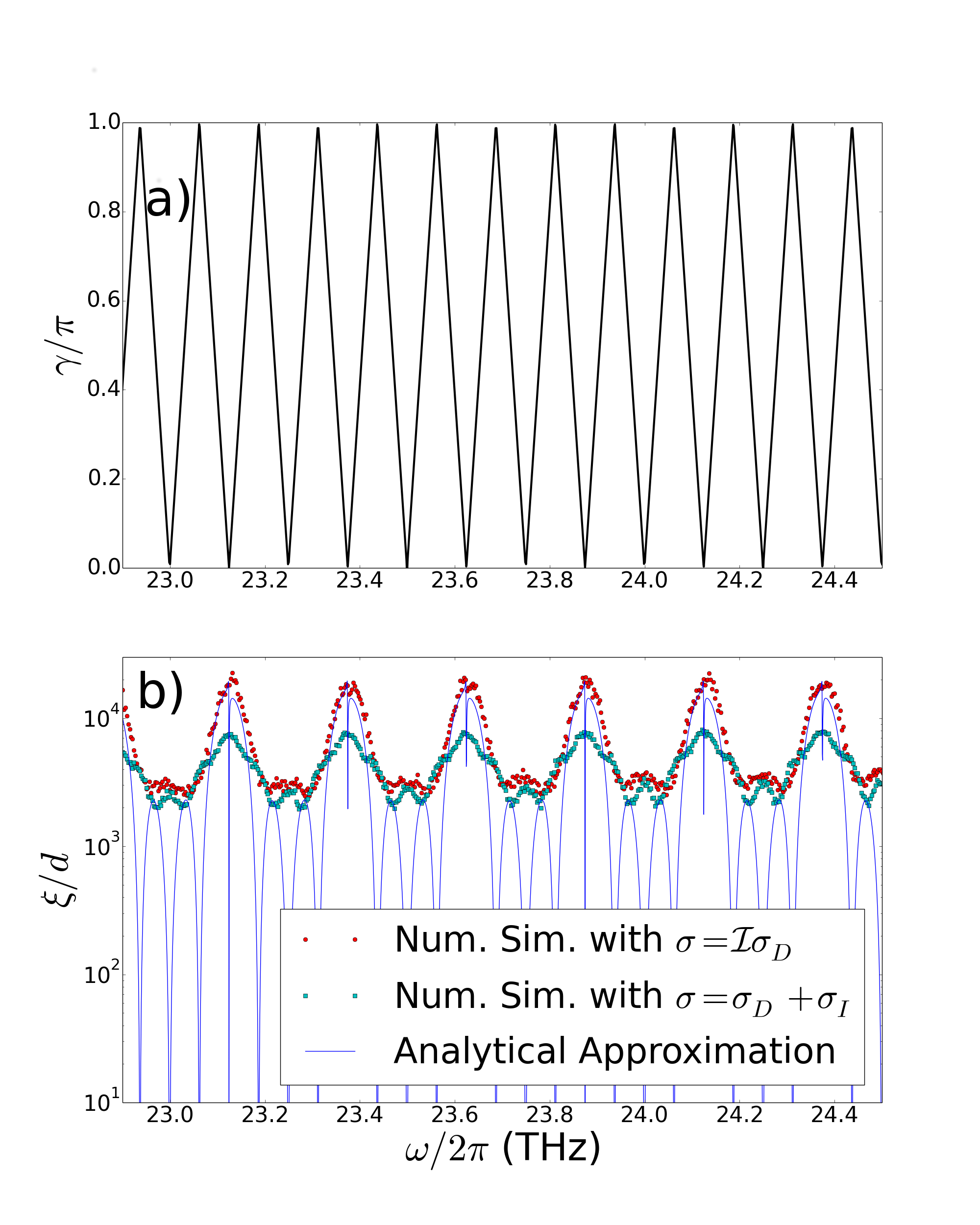
Figure 2: Color on-line. (a) Dispersion relation in the impedance matching regime and TM mode. (b) Localization length as a function of frequency with $\Upsilon_{i}=5\mu$m, $z_{i}^{0}=1.2$mm, $E_{F}=0.2$ eV, $\Gamma=260.\mu$eV, $N=5000$, $n_{\text{samples}}=100$, $\varepsilon_{1}=\mu_{1}=\mu_{2}=1$, $\varepsilon_{2}=3$, $\theta=\pi/3$.The solid line in (b) is the analytical result, whereas the dots correspond to two different numerical simulations for different regimes of the optical conductivity of graphene: (i) $\sigma=\Im m\sigma_{D}$ (red points) and (ii) $\sigma=\sigma_{D}+\sigma_{I}$ (blue points).

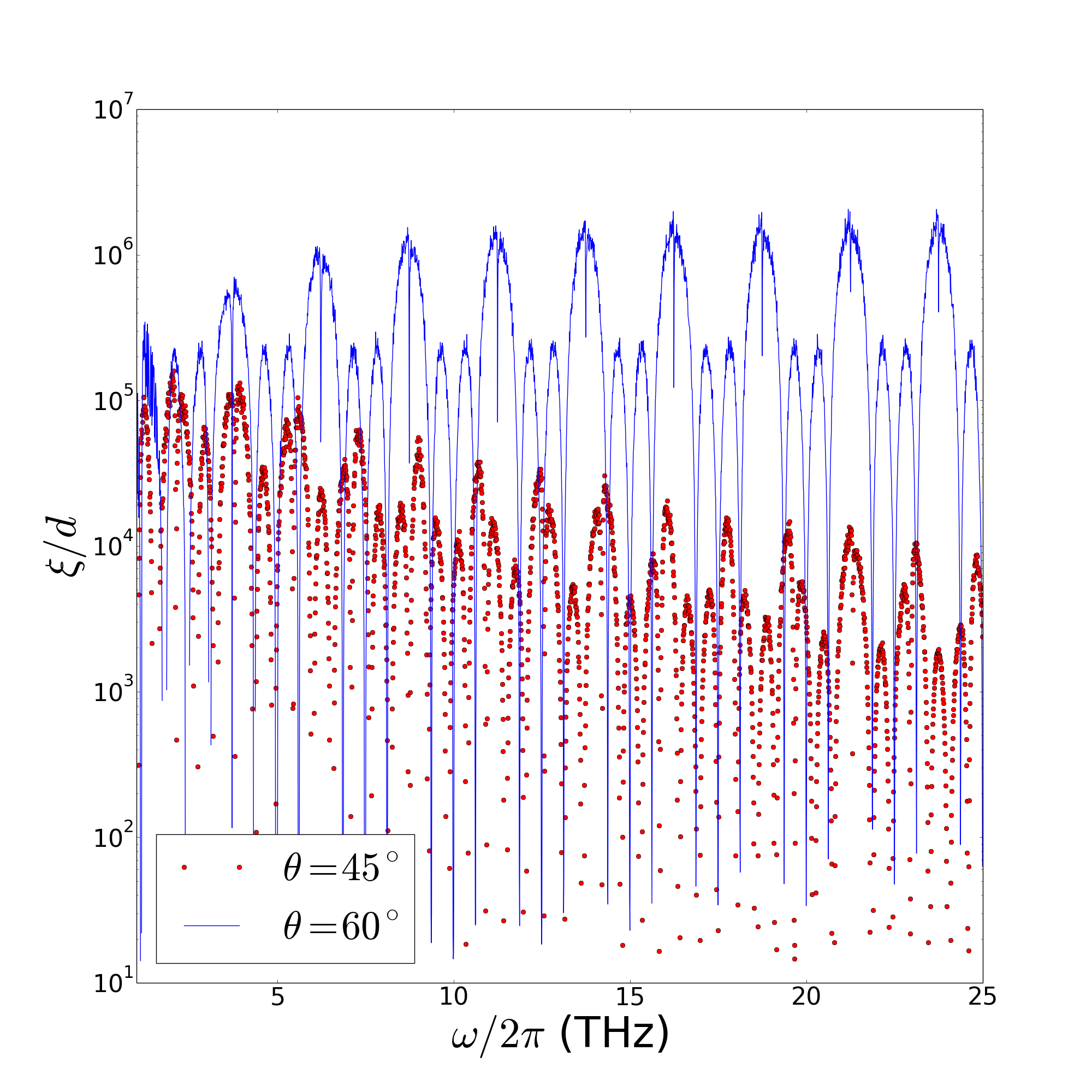
Figure 3: Color on-line. Localization length as a function of frequency in the impedance matched regime for two values of incidence angle: $\theta=60^{\circ}$ (blue line), $\theta=45^{\circ}$ (red circles). $\Upsilon_{i}=0.5\mu$m, $z_{i}^{0}=120\mu$m, $E_{F}=0.2$ eV, $\Gamma=0.\mu$eV, $N=5000$, $n_{\text{samples}}=100$.

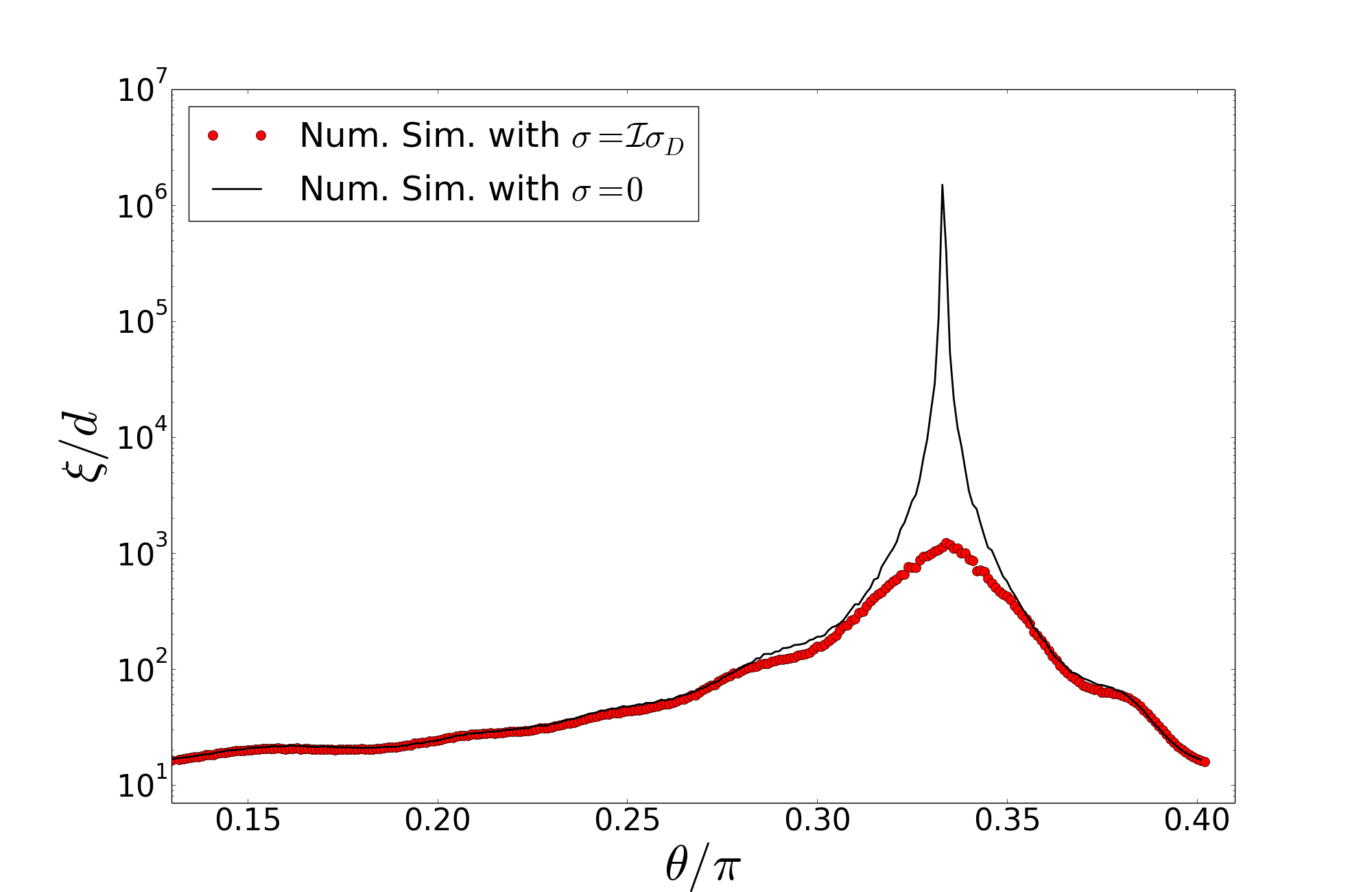
Figure 4: Color on-line. Localization length as a function of incidence angle in the impedance matched regime at the vicinities of a Brewster mode. $\Upsilon_{i}=50\mu$m, $z_{i}^{0}=120\mu$m, $N=5000$, $n_{\text{samples}}=100$. The black solid line corresponds to the grapheneless case; red circles correspond to the case where graphene is present in the superlattice ($E_{F}=0.2$ eV and $\Gamma=0\,$eV.)

III.3.2 ATR regime in one-layered system

The plasmon-polariton mode in graphene can be excited for example, by a prism in the Otto configuration [Bludov et al., 2010]. This is the regime we will explore in this section. We consider a periodic array of graphene/air unit cells (medium $2$) in between a dielectric (medium $1$). In this case the total transfer matrix $M$ is obtained considering the boundaries between the prism and the superlattice:

$$M=M_{1\rightarrow 2}\,\prod_{j}(M_{j})\,M_{2\rightarrow 1},$$ (31)

where $M_{1\rightarrow 2}$ refers to the transfer matrix describing light propagation from the medium $1$ (dielectric) to medium $2$ (air); $M_{2\rightarrow 1}$ refers to the reverse propagation. $M_{j}$ is the transfer matrix of the unit cell air/graphene with random widths (medium $2$).

From Eq. (55) one can see that for the evanescent mode $\alpha$ is a pure complex number and the first term in the right hand side becomes a hyperbolic cosine, which is greater than $1$ for any $\alpha$. As a result, the Bloch phase is real only if the second term in the right hand side of 55 is negative. This situation occurs for pure positive complex $f$; in this case $\beta$ is also a pure positive complex number, which is only possible in the TM mode [see Eqs. (32) and (52)].

For an incidence angle $\theta_{1}$ above the critical angle for total reflection at the interface $1/2$, a plasmon-polariton can be excited, allowing for frustrated total internal reflection. In this case light propagation occurs due to the presence of periodic graphene sheets. The effective impedance in the medium $2$ depends on the properties of the layer $1$ as:

$$Z_{2}^{\text{TE}}=i\frac{\kappa}{\mu_{2}},\,\,\,\,Z_{2}^{\text{TM}}=i\frac{\kappa}{\varepsilon_{2}},$$ (32)

where

$$\kappa=\sqrt{\varepsilon_{1}\mu_{1}\sin^{2}\theta_{1}-\varepsilon_{2}\mu_{2}}.$$ (33)

In Fig. 5 the localization length is calculated in the ATR regime using both numerical and analytical methods; the agreement is excellent. In the Drude regime $\xi$ is inversely proportional to the Fermi energy. Also shown is the localization length when the dielectric necessary to excite the ATR field is removed; we call this situation the normal field. The ATR field is characterized by exponentials with argument $\pm\omega\kappa z/c$. When the frequency increases and the length $c/\kappa\omega$ becomes smaller than the width $z$ of the dielectric slab (air in this case) light propagation comes to a halt, as the plasmon-polariton localized in a graphene layer cannot excite the adjacent layer. We can see that the ATR for the parameters of Fig. 5 fills the band gap of the normal field. Also the increase of disorder implies in the decrease of $\xi$, as expected.

Notice that ignoring the interband term and making $E_{F}=0$ is equivalent to remove the graphene sheets, therefore making disorder in random widths of air meaningless. Hence the localization length diverges, as can be seen in Eq. (24), where $\sigma\rightarrow 0$ implies in a vanishing Lyapunov exponent.

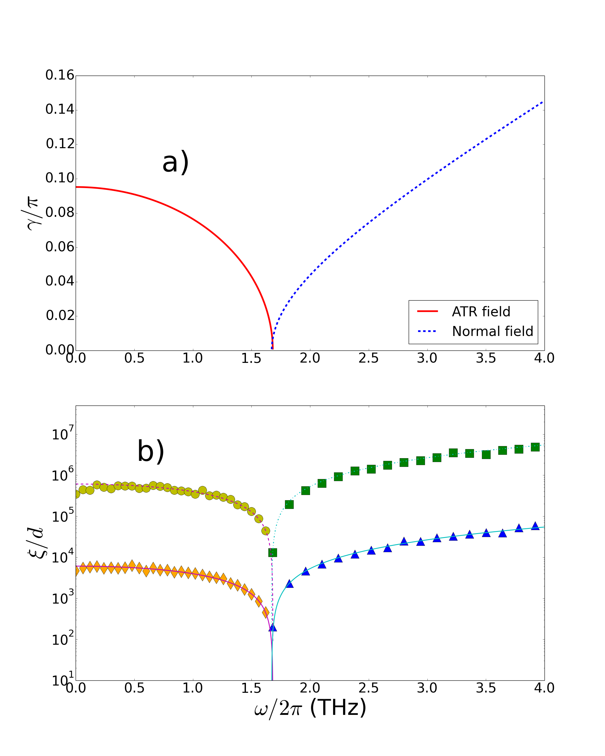
Figure 5: Color on-line. (a) Dispersion relation for the ATR regime (red) and for normal field (blue). (b) Localization length as a function of frequency for $z^{0}=12\mu$m, $E_{F}=0.1$ eV, $\theta_{1}=\pi/3$, $\varepsilon_{1}=2$,$\mu_{1}=\mu_{2}=\varepsilon_{1}=1$, $N=50000$, $n_{\text{samples}}=1$. The yellow circles (green squares) and orange diamonds (blue triangles) refer to the ATR (normal) field with $\Upsilon=0.5\mu$m and $\Upsilon=5\mu$m, respectively. The cyan and purple lines refer to the analytical approximation.

III.3.3 One layer system with compositional disorder

In the compositional disorder regime and for the one layered system, $\xi$ decreases as $\beta$ increases. For the TE mode, $\beta$ can only be greater than $1$ for materials with magnetic response, $\mu>1$. For the TM mode, $\beta$ is proportional to the dielectric constant and to $\cos\theta$, thus for grazing incidence, the system becomes fully opaque.

In the Drude regime the asymptotic behaviour of the localization length goes as $\omega^{2}$. This can be understood as follows: as the frequency increases the graphene conductivity decreases as $\omega^{-1}$ and thus the influence of the graphene layer disappears.

The effect of compositional disorder is shown in Fig. 6, where the Fermi energy is randomly distributed around the mean value $E_{F}^{0}=0.6$ eV. $\xi$ is inversely proportional to the mean standard deviation of the Fermi energy. We study the effect of increasing absorption in graphene layers, which depends on the real part of the conductivity and is proportional to the relaxation rate $\Gamma$. The length $\xi$ decays rapidly when the frequency reaches $2\omega_{F}$, and interband transitions start to occur, an effect that may be related either to absorption or to Anderson localization. The numerical calculation is performed with the full graphene conductivity (Drude plus interband) and then compared to the case where only the Drude term is present. The analytical approximation is calculated with the Drude term only, and agrees very well with the numerical simulation except at the band edges $\gamma=0,\pi/2,\pi$. As already discussed, this disagreement is related to the fact that the probability distribution of $\Theta_{n}$ is not uniform for these values of $\gamma$. The analytical approximation has a peak at $\gamma=\pi/2$ (see denominator of Eq. 22). The numerical calculations show that near the band gap ($\gamma=0,\pi$ see Eq. 22) $\xi$ goes to zero, and the peak at $\gamma=\pi/2$ does not occur.

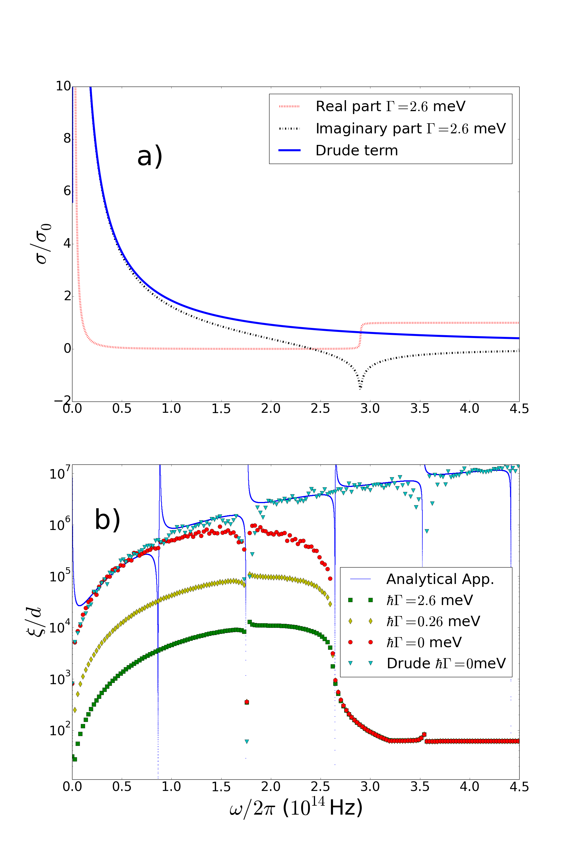
Figure 6: Color on-line. (a) Real and imaginary parts of the graphene optical conductivity in the compositional disordered case, $\sigma=\sigma_{D}+\sigma_{I}$, and the Drude conductivity $\sigma_{D}$ when $\Gamma=0$. (b) Localization length as a function of frequency with $z^{0}=1.2\mu$m, $\theta=\pi/4$, $\varepsilon=\mu=1$, $E_{F}^{0}=0.6$ eV, $\Upsilon_{F}=0.12$ eV, $N=5000$ and increasing relaxation rate $\Gamma$. $\omega_{F}\approx 3\times 10^{14}$ Hz. The blue triangles (and solid blue line) refer to a calculation where only the Drude conductivity with $\Gamma=0$ is used. The other data sets refer to the use of the full optical conductivity of graphene with different $\Gamma$ values.

III.4 Complex interband regime when: $\Re e\sigma\approx 0$, $\Im m\sigma<0$

When $\omega\lesssim 2\omega_{F}$, the imaginary part of the optical conductivity of graphene becomes negative and can be approximated by

$$\sigma=i\sigma_{I}^{\prime\prime}+i\sigma_{0}\frac{4}{\pi}\frac{\omega_{F}}{\omega},$$ (34)

where $\sigma_{I}^{\prime\prime}$ is given by Eq. (59). In this case the imaginary part of $\sigma$ becomes negative, and the ratio between the imaginary and real parts of $\sigma$ becomes lower than in the Drude regime for typical values of $\Gamma$ and $E_{F}$. Therefore, in this case the exponential decay of transmission is essentially due to absorption rather than to Anderson localization. Therefore, in this case, our approach for studying Anderson localization using the localization length is inadequate. It is worth commenting that experimentally it is possible to distinguish between absorption and Anderson localization by investigating the variance of the normalized total transmission, as proposed in Ref. [Chabanov et al., 2000]. For a one-layered system in the ATR regime with transfer matrix given by Eq. (54), the change in the sign of $f$ has qualitatively the same effect in the dispersion relation (55) of interchanging TE and TM modes, which changes the sign of $\beta$.

When the frequency becomes larger than $2\omega_{F}$, the real part of the conductivity approachs $\sigma_{0}$ while the imaginary part vanishs. In this regime, the role of the graphene sheets consists, essentially, in absorbing light leading to a vanishing transmission after few stacks.

IV Conclusions

In conclusion, we have investigated light propagation in 1D disordered superlattices composed of dielectric stacks and graphene sheets in between. We introduced disorder either in the graphene material parameters (compositional disorder), such as the Fermi energy, or in the widths of the dielectric stacks (structural disorder). For both cases we derived an analytical expression for the localization length $\xi$ and compared the results with numerical calculations based on the transfer matrix method. A very good agreement between numerics and the analytical expression was found. We demonstrated that, for structural disorder and when the impedances of the layers are equal, the localization length does not follow the well-known asymptotic behaviour $\xi\propto\omega^{-2}$. Rather, it exhibits an oscillatory dependence on frequency, as a result of the presence of the Drude term in the graphene conductivity. Also in the impedance matching regime, we show that graphene has an important impact on the Brewster modes, anomalously delocalised modes at given frequencies and incident angles at which $\xi$ diverges. Indeed, the presence of graphene induces additional reflections inside the disordered medium, leading to a strong attenuation of the Brewster modes. We investigated how intra and interband transitions in the graphene conductivity impact on $\xi$, identifying the regimes where Anderson localization and absorption dominates light transmission. Altogether, our findings unveil the role of graphene on Anderson localization of light, paving the way for the design of graphene-based, disordered photonic devices in the THz spectral range.

Appendix A Matrix transformation

The relation $\psi^{n+1}=M^{n}\psi^{n}$ can be interpreted as a discrete set of points in the phase space $\psi_{R},\psi_{L}$. With the transformation $M_{\text{real}}$:

$$M_{\text{real}}=\frac{1}{2}\begin{pmatrix}1-i&&1+i\\ -1+i&&1+i\end{pmatrix},$$ (35)

the matrix $M_{\text{real}}M^{n}M_{\text{real}}^{-1}$ is now real, and defining ${\psi^{\prime}}^{n}=M_{\text{real}}\psi^{n}$, we have in the phase space $\psi_{R}^{\prime},\psi_{L}^{\prime}$ that in the system without disorder the trajectory is given by a ellipse. From this we can find a transformation $M_{\text{circle}}$ to a circle:

$$M_{\text{circle}}=\begin{pmatrix}v^{-1}\cos\tau&&v\sin\tau\\ -v^{-1}\sin\tau&&v\cos\tau\end{pmatrix},$$ (36)

where:

$$v^{2}=-\frac{\sin\gamma}{\cosh\phi^{0}_{1}\sin\phi_{2}^{0}+\sinh\phi^{0}_{1}},$$

$$\tau=\frac{\pi}{4}-\frac{\phi_{3}^{0}}{2},$$ (37)

and making $[Q\,\,\,P]^{T}=M_{\text{circle}}\psi^{\prime}$,

$$\begin{pmatrix}Q_{n}\\ P_{n}\end{pmatrix}=\begin{pmatrix}v^{-1}\cos\tau&&v\sin\tau\\ -v^{-1}\sin\tau&&v\cos\tau\end{pmatrix}\begin{pmatrix}x_{n}\\ y_{n}\end{pmatrix},$$ (38)

Appendix B Lyapunov Exponent

The Lyapunov exponent is given by:

$$\lambda=\frac{1}{2}\left\langle Y_{1}+Y_{2}\cos 2\Theta_{n}+Y_{3}\sin 2\Theta_{n}-\frac{1}{4}Y_{2}^{2}-\frac{1}{4}Y_{3}^{2}\right\rangle,$$ (39)

where

$$Y_{1}=\frac{1}{\sin^{2}\gamma}\left[U_{1}\delta\phi_{1}^{2}+U_{2}\delta\phi_{2}^{2}+U_{3}\delta\phi_{3}^{2}+U_{4}\delta\phi_{1}\delta\phi_{2}\right],$$ (40)

with:

$$U_{1} = 2\sin^{2}\phi_{2}^{0},$$ (41)

$$U_{2} = 2\sinh^{2}\phi_{1}^{0}\cos^{2}\gamma,$$ (42)

$$U_{3} = 2\sinh^{2}\phi^{0}_{1}\sin^{2}\gamma,$$ (43)

$$U_{4} = -\sinh 2\phi^{0}_{1}\sin 2\phi_{2}^{0},$$ (44)

$$Y_{2}=\left[-2\sin\phi_{2}^{0}\delta\phi_{1}+\cos\phi_{2}^{0}\sinh 2\phi_{1}^{0}\left(\delta\phi_{2}-\delta\phi_{3}\right)\right],$$ (45)

$$Y_{3}=2\frac{\sinh\phi^{0}_{1}\left(\cos^{2}\gamma\delta\phi_{2}+\sin^{2}\gamma\delta\phi_{3}\right)-\cos\gamma\sin\phi_{2}^{0}\delta\phi_{1}}{-\sin\gamma}.$$ (46)

the angle $\Theta$ obeys the recurrence equation:

$$\Theta_{n+1}=\Theta_{n}-\gamma+\epsilon_{n}\csc\gamma,$$ (47)

with:

$$\epsilon_{n}= \left[\cos\gamma\sinh\phi^{0}_{1}\delta\phi_{2}-\sin\phi_{2}^{0}\delta\phi_{1}\right]\cos\left(2\Theta_{n}-\gamma\right)+$$ (48)

$$\sinh\phi^{0}_{1}\cos\gamma\sin(2\Theta_{n}-\gamma)\delta\phi_{3},$$

Appendix C Photonic Crystal

C.1 Unit cell made of two different dielectrics and a graphene sheet at the interfaces

The transfer matrix whose elements are Zhan et al. (2013)

$$m_{11}^{j} = \left[A^{x}_{-}\cos\alpha_{2}+i(\chi+C^{x}_{+})\sin\alpha_{2}\right]e^{-i\alpha_{1}},$$

$$m_{12}^{j} = \left[B^{x}\cos\alpha_{2}+i\left(\Delta+D^{x}\right)\sin\alpha_{2}\right]e^{i\alpha_{1}},$$

$$m_{21}^{j} = \left[-B^{x}\cos\alpha_{2}-i\left(\Delta+D^{x}\right)\sin\alpha_{2}\right]e^{-i\alpha_{1}},$$

$$m_{22}^{j} = \left[A^{x}_{+}\cos\alpha_{2}-i\left(\chi+C_{-}^{x}\right)\sin\alpha_{2}\right]e^{i\alpha_{1}},$$ (49)

where $x=\text{TE},\text{TM}$ and the diverse parameters are given in appendix C.

The Snell-Decartes law hold:

$$\sqrt{\varepsilon_{1}\mu_{1}}\sin\theta_{1}=\sqrt{\varepsilon_{2}\mu_{2}}\sin\theta_{2},$$ (50)

and the dispersion relation is given by:

$$\cos\gamma=\cos\alpha_{1}\cos\alpha_{2}-\left(\chi+2f^{2}\beta_{1}^{x}\beta_{2}^{x}\right)\sin\alpha_{1}\sin\alpha_{2}$$

$$+2if\left(\beta_{1}^{x}\cos\alpha_{1}\sin\alpha_{2}+\beta_{2}^{x}\cos\alpha_{2}\sin\alpha_{1}\right).$$ (51)

$$\beta_{i}^{TM}=Z_{i}^{TM}\,,\,\,\,\beta_{i}^{TE}=\frac{1}{Z_{i}^{TE}},$$ (52)

where:

$$k_{i} = \sqrt{\varepsilon_{i}\mu_{i}}\omega/c\cos\theta_{i},$$

$$\alpha_{i} = k_{i}z_{i},$$

$$A^{x}_{\pm} = (1\pm 2f\beta^{x}_{1}),$$

$$B^{x} = 2f\lambda^{x}\beta_{1}^{x},$$

$$C^{x}_{\pm} = \pm 2f\beta^{x}_{2}+2f^{2}\beta^{x}_{1}\beta^{x}_{2},$$

$$D^{x} = 2f^{2}\lambda^{x}\beta_{1}^{x}\beta_{2}^{x},$$

$$\eta^{x} = \frac{Z_{1}^{x}}{Z_{2}^{x}},$$

$$\Delta^{x} = \frac{1}{2}\left(\eta^{x}-{\eta^{x}}^{-1}\right),$$

$$\chi^{x} = \frac{1}{2}\left(\eta^{x}+{\eta^{x}}^{-1}\right),$$

$$f = \frac{\sigma c\mu_{0}}{2},$$

$$Z^{\text{TE}}_{i} = \frac{\sqrt{\mu_{i}\varepsilon_{i}}}{\mu_{i}}\cos\theta_{i},$$

$$Z^{\text{TM}}_{i} = \frac{\sqrt{\mu_{i}\varepsilon_{i}}}{\varepsilon_{i}}\cos\theta_{i},$$ (53)

with $\lambda^{\text{TM}}=+1,\lambda^{\text{TE}}=-1$.

C.2 Unit cell made of one dielectric and a graphene sheet at the interface

When there is only one dielectric, with width $z$ and $\varepsilon,\mu$ permissivity and permeability, intercalated by graphene sheets, the transfer matrix is given by:

$$M=\begin{pmatrix}(1-\beta^{x}f)e^{i\alpha}&&-\lambda^{x}\beta^{x}fe^{i\alpha}\\ \lambda^{x}\beta^{x}fe^{-i\alpha}&&(1+\beta^{x}f)e^{-i\alpha}\end{pmatrix},$$ (54)

where $\alpha=\sqrt{\mu\varepsilon}z\cos\theta$ with the dispersion relation:

$$\cos\gamma=\cos\alpha-i\beta^{x}f\sin\alpha.$$ (55)

Appendix D Graphene Optical Conductivity

For completeness we give here the expressions for the optical conductivity of graphene, whose derivation can be found elsewhere Peres (2010); Bludov et al. (2013b). The graphene optical conductivity of graphene is a sum of a Drude term, $\sigma_{D}$, and an inter-band contribution, $\sigma_{I}$, reading:

$$\sigma=\sigma_{D}+\sigma_{I},$$ (56)

where the Drude term is given by:

$$\frac{\sigma_{D}}{\sigma_{0}}=\frac{4\omega_{F}}{\pi}\frac{1}{\Gamma-i\omega},$$ (57)

and the interband term $\sigma_{I}=\sigma_{I}^{\prime}+i\sigma^{\prime\prime}_{I}$ have the real part

$$\frac{\sigma_{I}^{\prime}}{\sigma_{0}}=\left(1+\frac{1}{\pi}\arctan\frac{\omega-2\omega_{F}}{\Gamma}-\frac{1}{\pi}\arctan\frac{\omega+2\omega_{F}}{\Gamma}\right),$$ (58)

and the imaginary part

$$\frac{\sigma_{I}^{\prime\prime}}{\sigma_{0}}=-\frac{1}{2\pi}\ln\frac{(2\omega_{F}+\omega)^{2}+\Gamma^{2}}{(2\omega_{F}-\omega)^{2}+\Gamma^{2}},$$ (59)

with the Fermi frequency given by

$$\omega_{F}=\frac{|E_{F}|}{\hbar}.$$ (60)

References

- Avouris and Freitag (2014) P. Avouris and M. Freitag, IEEE Journal of Selected Topics in Quantum Electronics 20, 72 (2014).
- Bludov et al. (2013a) Y. V. Bludov, N. M. R. Peres, and M. I. Vasilevskiy, J. of Opt. 15, 114004 (2013a).
- Zhan et al. (2013) T. Zhan, X. Shi, Y. Dai, X. Liu, and J. Zi, J. of Phys.: Cond. Matt. 25, 215301 (2013).
- Xia et al. (2009) F. Xia, T. Mueller, Y. Lin, A. Valdes-Garcia, and P. Avouris, Nat. Nanotechnol. 4, 839 (2009).
- Liu et al. (2011) M. Liu, X. Yin, E. Avila, B. Geng, T. Zentgraf, L. Ju, F. Wang, and X. Zhang, Nature 474, 64 (2011).
- Garcia de Abajo (2014) F. Garcia de Abajo, ACS Photonics 1, 135 (2014).
- Ju et al. (2011) L. Ju, B. Geng, J. Horng, C. Girit, M. Martin, Z. Hao, H. Bechtel, X. Liang, A. Zettl, Y. Shen, and F. Wang, Nat. Nanotechnol. 6, 630 (2011).
- Echtermeyer et al. (2011) T. Echtermeyer, L. Britnell, P. Jasnos, A. Lombardo, R. Gorbachev, A. Grigorenko, A. Geim, A. Ferrari, and K. Novoselov, Nat. Commun. 2, 458 (2011).
- Sun et al. (2010) Z. Sun, T. Hasan, F. Torrisi, D. Popa, G. Privitera, F. Wang, F. Bonaccorso, D. Basko, and A. Ferrari, ACS Nano 4, 803 (2010).
- Engel et al. (2012) M. Engel, M. Steiner, A. Lombardo, A. Ferrari, H. Lohneysen, P. Avouris, and R. Krupke, Nat Commun. 3, 906 (2012).
- Majumdar et al. (2013) A. Majumdar, J. Kim, J. Vuckovic, and F. Wang, Nano Lett. 92, 68001 (2013).
- Gan et al. (2013) X. Gan, R. Shiue, Y. Gao, K. Mak, X. Yao, L. Li, A. Szep, D. Walker, J. Hone, T. Heinz, and D. Englund, Nano Lett. 13, 69 (2013).
- Anderson (1958) P. Anderson, Phys. Rev. 109, 1492 (1958).
- Segev et al. (2013) M. Segev, Y. Silberberg, and D. Christodoulides, Nature Photon. 7, 197 (2013).
- Hu et al. (2008) H. Hu, A. Strybulevych, J. Page, S. Skipetrov, and B. van Tiggelen, Nature Phys. 4, 945 (2008).
- Billy et al. (2008) J. Billy, V. Josse, Z. Zuo, A. Bernard, B. Hambrecht, P. Lugan, D. Clement, L. Sanchez-Palencia, P. Bouyer, and A. Aspect, Nature 453, 891 (2008).
- Lagendijk et al. (2009) A. Lagendijk, B. van Tiggelen, and D. Wiersma, Physics Today 62, 24 (2009).
- Izrailev et al. (2012) F. Izrailev, A. Krokhin, and N. Makarov, Physics Reports 512, 125 (2012).
- Bertolotti et al. (2005) J. Bertolotti, S. Gottardo, D. Wiersma, M. Ghulinyan, and L. Pavesi, Phys. Rev. Lett. 94, 113903 (2005).
- Mogilevtsev et al. (2010) D. Mogilevtsev, F. A. Pinheiro, R. R. dos Santos, S. B. Cavalcanti, and L. E. Oliveira, Phys. Rev. B 82, 081105 (2010).
- Mogilevtsev et al. (2011) D. Mogilevtsev, F. A. Pinheiro, R. R. dos Santos, S. B. Cavalcanti, and L. E. Oliveira, Phys. Rev. B 84, 094204 (2011).
- Asatryan et al. (2007) A. A. Asatryan, L. C. Botten, M. A. Byrne, V. D. Freilikher, S. A. Gredeskul, I. V. Shadrivov, R. C. McPhedran, and Y. S. Kivshar, Phys. Rev. Lett. 99, 193902 (2007).
- Kuzmiak and Maradudin (1997) V. Kuzmiak and A. Maradudin, Physical Review B 55, 7427 (1997).
- Soto-Puebla et al. (2004) D. Soto-Puebla, F. Ramos-Mendieta, and M. Xiao, International Journal of Modern Physics B 18, 125 (2004).
- Markos and Soukoulis (2008) P. Markos and C. M. Soukoulis, Wave Propagation: From electrons to photonic crystals and left-handed materials (Princeton University Press, 2008).
- Izrailev and Makarov (2009) F. M. Izrailev and N. M. Makarov, Phys. Rev. Lett. 102, 203901 (2009).
- Izrailev et al. (1995) F. M. Izrailev, T. Kottos, and G. P. Tsironis, Phys. Rev. B 52, 3274 (1995).
- Izrailev et al. (1998) F. M. Izrailev, S. Ruffo, and L. Tessieri, J. Phys. A 31, 5263 (1998).
- Sipe et al. (1988) J. E. Sipe, P. Sheng, B. S. White, and M. H. Cohen, Phys. Rev. Lett. 60, 108 (1988).
- Bludov et al. (2010) Y. V. Bludov, M. Vasilevskiy, and N. Peres, EPL (Europhysics Letters) 92, 68001 (2010).
- Chabanov et al. (2000) A. A. Chabanov, M. Stoytchev, and A. Z. Genack, Nature 404, 850 (2000).
- Note (1) There are some typos in the transfer matrix elements given in reference Zhan et al. (2013).
- Peres (2010) N. M. R. Peres, Rev. of Mod. Phys. 82, 2673 (2010).
- Bludov et al. (2013b) Y. V. Bludov, A. Ferreira, N. M. R. Peres, and M. I. Vasilevskiy, Int. J. of Mod. Phys. B 27, 1341001 (2013b).