On Some Basic Results Related to Affine Functions on Riemmanian Manifolds

Abstract. We study some basic properties of the function $f_{0}:M\rightarrow{\mathbb{R}}$ on Hadamard manifolds defined by

$$f_{0}(x):=\langle u_{0},\exp_{x_{0}}^{-1}x\rangle\quad\mbox{for any $x\in M$}.$$

A characterization for the function to be linear affine is given and a counterexample on Poincaré plane is provided, which in particular, shows that assertions (i) and (ii) claimed in [11, Proposition 3.4] are not true, and that the function $f_{0}$ is indeed not quasi-convex. Furthermore, we discuss the convexity properties of the sub-level sets of the function on Riemannian manifolds with constant sectional curvatures.

Keywords. Riemannian manifold; Hadamard manifold; sectional curvature; convex function; quasiconvex function; linear affine function

1 Introduction

Let $M$ be a Hadamard manifold and let $x\in M$. Let $T_{x}M$ stand for the tangent space at $x$ to $M$ with the Riemannian scalar product denoted by $\langle\cdot,\cdot\rangle_{x}$ and let $TM:=\cup_{x\in M}T_{x}M$. We use $\exp_{x}$ and $P_{x,x_{0}}$, where $x_{0}\in M$, to denote the exponential map of $M$ at $x$ and the parallel transport from $x_{0}$ to $x$ (along the unique geodesic joining $x_{0}$ to $x$), respectively. Now fix $x_{0}\in M$ and $u_{0}\in T_{x_{0}}M\setminus\{0\}$. Consider the vector field $X_{0}:M\to TM$ and the function $f_{0}:M\rightarrow{\mathbb{R}}$ defined by

$$X_{0}(x):=P_{x,x_{0}}u_{0}\quad\quad\mbox{for any $x\in M$}$$ (1.1)

and

$$f_{0}(x):=\langle u_{0},\exp_{x_{0}}^{-1}x\rangle\quad\mbox{for any $x\in M$},$$ (1.2)

respectively. Let ${\rm grad}f_{0}$ denote the gradient of $f_{0}$. Assertions (a) and (b) below were given in [11, Proposition 3.4] (without the proof for (b)).

(a) ${\rm grad}f_{0}=X_{0}$.

(b) $f_{0}$ is linear affine on $M$.
Recently, assertions (a) and (b) have been used in [11, 12] to study the proximal point algorithm for quasiconvex/convex functions with Bregman distances on Hadamard manifolds; while assertion (b) was also used in [3, 19] to establish some existence results of solutions for Equilibrium problems and vector optimization problems on Hadamard manifolds, respectively. However, assertion (b) is clearly not true in general because, by [14, p. 299, Theorem 2.1]), any twice differentiable linear affine function on Poincaré plane ${\mathbb{H}}$ (a two dimensional Hadamard manifold of constant curvature $-1$) is constant. Indeed, it has been further shown in [7, Theorem 2.1] that assertion (b) is true for any $x_{0}\in M$ and $u_{0}\in T_{x_{0}}M$ if and only if $M$ is isometric to the Euclidean space ${\mathbb{R}}^{n}$. Furthermore, one can easily check that the function $f_{0}$ defined by (1.2) is even not convex, in general, because, otherwise, one has that both $f_{0}$ and $-f_{0}$ are convex (and so linear affine). This motivates us to consider the following problem:

Problem 1 Is the function $f_{0}$ defined by (1.2) quasi-convex?

Let $\nabla$ denote the Riemannian connection on $M$ and let $\mathcal{X}(M)$ denote all $C^{\infty}$ vector field on $M$. Recall from [14, P.83] that a smooth function $f:M\rightarrow{\mathbb{R}}$ is linear affine if and only if

$$\nabla_{X}{\rm grad}\,f=0\quad\mbox{for any $X\in\mathcal{X}(M)$}.$$

Specializing in the function $f_{0}$ defined by (1.2), one is motivated to consider the following problems:

Problem 2 Is assertion (a) true?

Problem 3 Does the vector field $X_{0}$ defined by (1.1) satisfy

$$\nabla_{X}X_{0}=0\quad\mbox{for any $XY\in\mathcal{X}(M)$}?$$ (1.3)

The first purpose of this paper is to present a characterization in Hadamard manifolds for (b) to be true in terms of assertion (a) and the parallel transports, and to provide a counterexample on Poincaré plane to illustrate that the answer to each of Problems 1-3 is negative. In particular for Problem 2, we show that the vector field $X_{0}$ defined by (1.1) is even not a gradient field.

Our second purpose in the present paper is, in spirit of the negative answer to Problem 1, to study the convexity issue of sub-level sets of the function $f_{0}$ defined by (1.2) in Riemannian manifolds with constant sectional curvatures. Our main results provide the exact estimate of the constant $c$ such that the sub-level set $L_{c,f_{0}}:=\{x\in M:f_{0}(x)\leq c\}$ is strongly convex, which in particular improves and extends the corresponding result in [6, Corollary 3.1].

The paper is organized as follows. We review, in Section 2, some basic notions, notations and some classical results of Riemannian geometry that will be needed afterward. The characterization in Hadamard manifolds for (b) to be true and the counterexample on Poincaré plane are presented in Section 3. Finally, in Section 4, the convexity properties of the sub-level sets of the functions defined by (1.2) in Riemannian manifolds with constant sectional curvatures are discussed.

2 Notations, notions and preliminaries

In present section, we present some basic notations, definitions and properties of Riemannian manifolds. The readers are referred to some textbooks for details, for example, [4, 13, 14].

Let $M$ be a connected $n$-dimensional Riemannian manifold with the Levi-Civita connection $\nabla$ on $M$. We denote the tangent space at $x\in M$ by $T_{x}M$ and Let $\mathcal{X}(M)$ denote all ($C^{\infty}$) vector fields on $M$. By $\langle\cdot,\cdot\rangle_{x}$ and $\|\cdot\|_{x}$ we mean the corresponding Riemannian scalar product and the norm, respectively (where the subscript $x$ is sometimes omitted). For $x,y\in{M}$, let $\gamma:[0,1]\rightarrow M$ be a piecewise smooth curve joining $x$ to $y$. Then, the arc-length of $\gamma$ is defined by $l(\gamma):=\int_{0}^{1}\|\dot{\gamma}(t)\|{\rm d}t$, while the Riemannian distance from $x$ to $y$ is defined by ${\rm d}(x,y):=\inf_{\gamma}l(\gamma)$, where the infimum is taken over all piecewise smooth curves $\gamma:[0,1]\rightarrow M$ joining $x$ to $y$. We use ${\mathbb{B}}(x,r)$ to denote the open metric ball at $x$ with radius $r$, that is,

$${\mathbb{B}}(x,r):=\{y\in M:{\rm d}(x,y)<r\}.$$

For a smooth curve $\gamma$, if $\dot{\gamma}$ is parallel along itself, then $\gamma$ is called a geodesic, that is, a smooth curve $\gamma$ is a geodesic if an only if $\nabla_{\dot{\gamma}}{\dot{\gamma}}=0$. A geodesic $\gamma:[0,1]\rightarrow M$ joining $x$ to $y$ is minimal if its arc-length equals its Riemannian distance between $x$ and $y$. By the Hopf-Rinow theorem [4], $(M,{\rm d})$ is a complete metric space, and there is at least one minimal geodesic joining $x$ to $y$. The set of all geodesics $\gamma:[0,1]\rightarrow M$ with $\gamma(0)=x$ and $\gamma(1)=y$ is denoted by $\Gamma_{xy}$, that is

$$\Gamma_{xy}:=\{\gamma:[0,1]\rightarrow M:\;\gamma(0)=x,\,\gamma(1)=y\mbox{ and }\nabla_{\dot{\gamma}}\dot{\gamma}=0\}.$$

Let $\gamma$ be a geodesic. We use $P_{\gamma,\cdot,\cdot}$ to denote the parallel transport on the tangent bundle $TM$ (defined below) along $\gamma$ with respect to $\nabla$, which is defined by

$$P_{\gamma,\gamma(b),\gamma(a)}v=X(\gamma(b))\quad\mbox{for all }a,b\in{\mathbb{R}}\mbox{ and }v\in T_{\gamma(a)}M,$$ (2.1)

where $X$ is the unique vector field satisfying

$$X(\gamma(a))=v\quad\mbox{and}\quad\nabla_{\dot{\gamma}}X=0.$$ (2.2)

Then, for any $a,b\in{\mathbb{R}}$, $P_{\gamma,\gamma(b),\gamma(a)}$ is an isometry from $T_{\gamma(a)}M$ to $T_{\gamma(b)}M$. We will write $P_{y,x}$ instead of $P_{\gamma,y,x}$ in the case when $\gamma$ is a minimal geodesic joining $x$ to $y$ and no confusion arises.

The exponential map of $M$ at $x\in M$ is denoted by $\exp_{x}(\cdot):T_{x}M\rightarrow M$. For a $C^{\infty}$ function $f:M\rightarrow{\mathbb{R}}$, ${\rm grad}f$ and ${\rm Hess}f$ denote its gradient vector and Hessian, respectively. Let $X,Y\in\mathcal{X}(M)$. The Riemannian connection has the expression in terms of parallel transportation, that is,

$$(\nabla_{X}Y)(x)=\lim_{t\rightarrow 0}\frac{1}{t}\{P_{\gamma,\gamma(t),\gamma(0)}Y(\gamma(t))-Y(x)\}\quad\mbox{for any $x\in M$},$$ (2.3)

where the curve $\gamma$ with $\gamma(0)=x$ and $\dot{\gamma}(0)=X(x)$ (see, e.g., [13, p. 29 Exercise 5]).

A complete simply connected Riemannian manifold of non-positive sectional curvature is called a Hadamard manifold. The following propositions are well-known about the Hadamard manifolds, see, e.g, [13, p. 221].

Proposition 2.1.

Suppose that $M$ is a Hadamard manifold. Let $p\in M$. Then, $\exp_{p}:T_{p}M\rightarrow M$ is a diffeomorphism, and for any two points $p,q\in M$ there exists a unique normal geodesic joining $p$ to $q$, which is in fact a minimal geodesic.

The following definition presents the notions of different convexities, where item (a) and (b) are known in [2]; see also [8, 15, 16].

Definition 2.1.

Let $Q$ be a nonempty subset of the Riemannian manifold $M$. Then, $Q$ is said to be

(a) weakly convex if, for any $x,y\in Q$, there is a minimal geodesic of $M$ joining $x$ to $y$ and it is in $Q$;

(b) strongly convex if, for any $x,y\in Q$, there is just one minimal geodesic of $M$ joining $x$ to $y$ and it is in $Q$.

All convexities in a Hadamard manifold coincide and are simply called the convexity. Let $f:M\rightarrow\overline{{\mathbb{R}}}$ be a proper function, and let ${\rm dom}f$ denote its domain, that is, ${\rm dom}f:=\{x\in M:f(x)\neq\infty\}$. We use $\Gamma^{f}_{xy}$ to denote the set of all $\gamma\in\Gamma_{xy}$ such that $\gamma\subseteq{\rm dom}f$. In the following definition, item (a) is known in [9, 10] and item (b) is an extension of the one in [14, p. 59], which is introduced for the case when ${\rm dom}f$ is totally convex.

Definition 2.2.

Let $f:M\rightarrow\overline{{\mathbb{R}}}$ be a proper function and suppose that ${\rm dom}f$ is weakly convex. Then, $f$ is said to be

(a) convex if

$$f\circ\gamma(t)\leq(1-t)f(x)+tf(y)\quad\mbox{for all }x,y\in{\rm dom}f,\;\gamma\in\Gamma_{xy}^{f},\;t\in[0,1];$$

(b) quasi-convex if

$$f\circ\gamma(t)\leq\max\{f(x),f(y)\}\quad\mbox{for all }x,y\in{\rm dom}f,\;\gamma\in\Gamma_{xy}^{f},\;t\in[0,1].$$

Clearly, for a proper function $f$ with a weakly convex domain, the convexity implies the quasi-convexity. Fixing $c\in{\mathbb{R}}$, we use $L_{c,f}$ to denote the sub-level set of $f$ defined by

$$L_{c,f}:=\{x\in M:f(x)\leq c\}.$$

The following proposition describe the relationship between the convexities of a function $f$ and its sub-level sets.

Proposition 2.2.

Let $f:M\rightarrow\overline{{\mathbb{R}}}$ be a proper function with weakly convex domain ${\rm dom}f$. Then, $f$ is quasi-convex if and only if, for each $c\in{\mathbb{R}}$, the sub-level set $L_{c,f}$ is totally convex with restricted to ${\rm dom}f$ in the sense that for any $x,y\in L_{c,f}$, if $\gamma\in\Gamma^{f}_{xy}$ then $\gamma\subseteq L_{c,f}$. In particular, $f$ is quasi-convex if and only if $L_{c,f}$ is strongly convex for each $c\in{\mathbb{R}}$ in the case when ${\rm dom}f$ is strongly convex.

Proof.

We only consider the case when ${\rm dom}f$ is weakly convex (otherwise when ${\rm dom}f$ is weakly convex, the result is immediate by definition).

Suppose that $f$ is quasi-convex. Take $c\in{\mathbb{R}}$. Let $x,y\in L_{c,f}\subseteq{\rm dom}f$ and let $\gamma\in\Gamma_{xy}^{f}$ (i.e., $\gamma$ is a geodesic joining $x$ to $y$ which is contained in ${\rm dom}f$). Then, $f(x)\leq c$ and $f(y)\leq c$. Noting that $f$ is quasi-convex, it follows that

$$f\circ\gamma(t)\leq\max\{f(x),f(y)\}\leq c\quad\mbox{for all }t\in[0,1].$$

This implies that $\gamma\subseteq L_{c,f}$ and so $L_{c,f}$ is totally convex restricted to ${\rm dom}f$ since $x,y\in L_{c,f}$ and $\gamma\in\Gamma_{xy}^{f}$ are arbitrary.

Conversely, suppose that $L_{c,f}$ is totally convex restricted to ${\rm dom}f$ for each $c\in{\mathbb{R}}$. Let $x,y\in{\rm dom}f$ and let $\gamma\in\Gamma_{xy}^{f}$. Set $c_{0}:=\max\{f(x),f(y)\}$. Then, by assumption, $\gamma\subseteq L_{c_{0},f}$, that is,

$$f\circ\gamma(t)\leq c_{0}=\max\{f(x),f(y)\}\quad\mbox{for all $t\in[0,1]$}.$$

This implies that $f$ is quasi-convex since $x,y\in{\rm dom}f$ and $\gamma\in\Gamma_{xy}^{f}$ are arbitrary. The proof is complete. ∎

3 Linear affine functions and counterexample on Hadamard manifolds

For the whole section, we assume that $M$ is a Hadamard manifold. Consider a proper convex function $f:M\rightarrow\overline{{\mathbb{R}}}$ on $M$. We define the subdifferential of $f$ at $x\in{\rm dom}f$ by

$$\partial f(x):=\{v\in T_{x}M:\;f(y)\geq f(x)+\langle v,\gamma^{\prime}(0)\rangle\;\;\mbox{ for all }y\in{\rm dom}f\mbox{ and }\gamma\in\Gamma^{f}_{xy}\}.$$

By [14, p. 74] (see also [10, Proposition 6.2]), $\partial f(x)$ is a nonempty, compact and convex set for any $x\in{\rm int}({\rm dom}f)$, where ${\rm int}Q$ denotes the topological interior of a subset $Q$ of $M$. Let $f:M\rightarrow\overline{{\mathbb{R}}}$ be a proper function with convex domain. Recall that $f$ is linear affine if both $f$ and $-f$ are convex. Furthermore, if $f$ is of $C^{2}$ and ${\rm dom}f$ is open, its second covariant differetial ${\rm Hess}f$ is defined by

$${\rm Hess}f(X,Y)=\langle\nabla_{X}{\rm grad}f,Y\rangle\quad\mbox{for any }X,Y\in\mathcal{X}(M).$$

Then $f$ is linear affine if and only if ${\rm Hess}f=0$ on ${\rm dom}f$; see [14, P.83]. The following theorem present, in particular, a characterization in Hadamard manifolds for assertion (b) to be true in terms of assertion (a) and the parallel transports.

Theorem 3.1.

Let $f:M\rightarrow\overline{{\mathbb{R}}}$ be a proper function and suppose that ${\rm dom}f$ is a nonempty open convex subset. If function $f$ is linear affine, then, for any $x_{0}\in{\rm dom}f$, there exists $u_{0}\in T_{x_{0}}M$ such that

$$P_{x,x_{0}}u_{0}=P_{x,z}\circ P_{z,x_{0}}u_{0}\quad\mbox{for any }(z,x)\in{\rm dom}f\times{\rm dom}f,$$ (3.1)

$${\rm grad}f(x)=P_{x,x_{0}}u_{0}\quad\mbox{for any }x\in{\rm dom}f$$ (3.2)

and

$$f(x)=f(x_{0})+\langle u_{0},\exp_{x_{0}}^{-1}x\rangle\quad\mbox{for any }x\in{\rm dom}f.$$ (3.3)

Conversely, if there exist $x_{0}\in{\rm dom}f$ and $u_{0}\in T_{x_{0}}M$ such that (3.1) and (3.2) hold, then $f$ is linear affine.

Proof.

Assume that $f$ is linear affine. Then both $f$ and $-f$ are convex. Take $x_{0}\in{\rm dom}f$ and note that ${\rm dom}f$ is open. It follows that both $\partial f(x_{0})$ and $\partial(-f(x_{0}))$ are nonempty. Thus one can chose $u_{0}\in\partial f(x_{0})$ and $u_{0}^{\prime}\in\partial(-f(x_{0}))$, respectively. Then, by definition, we have that, for any $x\in{\rm dom}f$,

$$\begin{array}[]{ll}f(x)\geq f(x_{0})+\langle u_{0},\exp_{x_{0}}^{-1}x\rangle\quad\mbox{and}\quad-f(x)\geq-f(x_{0})+\langle u_{0}^{\prime},\exp_{x_{0}}^{-1}x\rangle;\end{array}$$ (3.4)

hence $\langle u_{0}+u_{0}^{\prime},\exp_{x_{0}}^{-1}x\rangle_{x_{0}}\leq 0$ for any $x\in{\rm dom}f$. This implies that $u_{0}+u_{0}^{\prime}=0$, that is $u_{0}^{\prime}=-u_{0}$ (as ${\rm dom}f$ is open). Thus (3.3) follows from (3.4). Furthermore, noting that $f$ is of class $C^{\infty}$ by (3.3), one then has that ${\rm Hess}f=0$ on ${\rm dom}f$, that is,

$$\mbox{${\rm Hess}f(X,Y)=\langle\nabla_{X}{\rm grad}f,Y\rangle=0$\;\; for any $X,Y\in\mathcal{X}({\rm dom}f)$}.$$

In particular, one has that

$$\nabla_{\dot{\gamma}_{xz}}{\rm grad}f=0\quad\mbox{for any }x,z\in{\rm dom}f,$$

where ${\gamma}_{xz}$ is the geodesic joining $x$ and $z$, which lies in ${\rm dom}f$. This, together with the definition of parallel transport (e.g., (2.1)), implies that

$${\rm grad}f(x)=P_{x,z}{\rm grad}f(z)\quad\mbox{for any }x,z\in{\rm dom}f.$$ (3.5)

Note further that, for any $u\in T_{x_{0}}M$, one has

$$\langle{\rm grad}f(x_{0}),u\rangle_{x_{0}}=\frac{{\rm d}}{{\rm d}t}f\circ\exp_{x_{0}}tu\mid_{t=0}=\langle u_{0},u\rangle_{x_{0}}.$$

It follows that ${\rm grad}f(x_{0})=u_{0}$. This, together with (3.5), implies that (3.1) and (3.2) hold.

Now, suppose that (3.1) and (3.2) hold for some $x_{0}\in{\rm dom}f$ and $u_{0}\in T_{x_{0}}M$. Let $x\in{\rm dom}f$ and $X\in\mathcal{X}({\rm dom}f)$. Let $\gamma:[-\varepsilon,\varepsilon]\rightarrow{\rm dom}f$ be the geodesic contained in ${\rm dom}f$ with $\gamma(0)=x$ and $\dot{\gamma}(0)=X(x)$. Let $t\in[-\varepsilon,\varepsilon]$. We see from (3.2) that

$${\rm grad}f(x)=P_{x,x_{0}}u_{0},\;{\rm grad}f(\gamma(t))=P_{\gamma(t),x_{0}}u_{0}.$$

In light of (3.1), it follows that

$$P_{x,\gamma(t)}{\rm grad}f(\gamma(t))=P_{x,\gamma(t)}\circ P_{\gamma(t),x_{0}}u_{0}=P_{x,x_{0}}u_{0}={\rm grad}f(x).$$

Noting that $P_{x,\gamma(t)}=P_{\gamma,x,\gamma(t)}$, one gets by (2.3) that

$$(\nabla_{X}{\rm grad}f)(x)=\lim_{t\rightarrow 0}\frac{1}{t}\{P_{x,\gamma(t)}{\rm grad}f(\gamma(t))-{\rm grad}f(x)\}=0.$$

Since $X\in\mathcal{X}({\rm dom}f)$ and $x\in{\rm dom}f$ are arbitrary, we conclude that ${\rm Hess}f=0$ on ${\rm dom}f$, and so $f$ is linear affine. The proof is complete. ∎

The remainder of this section is to construct a counterexample on Poincaré plane to illustrate that the answer to each of Problems 1-3 is negative. To do this, let

$$M={\mathbb{H}}=:\{(t_{1},t_{2})\in\mathbb{R}^{2}|\ t_{2}>0\},$$

be the Poincaré plane endowed with the Riemannian metric, in terms of the natural coordinate system, defined by

$$g_{11}=g_{22}:=\frac{1}{t_{2}^{2}},\ g_{12}:=0\text{ for each }(t_{1},t_{2})\in{\mathbb{H}}.$$ (3.6)

The sectional curvature of ${\mathbb{H}}$ is equal to $-1$ (see, e.g., [4, p. 160]), and the geodesics on ${\mathbb{H}}$ are the semilines $\gamma(a;\cdot):=(\gamma^{1}(a;\cdot),\gamma^{2}(a;\cdot))$ (through $(a,1)$), and the semicircles $\gamma(b,r;\cdot):=(\gamma^{1}(b,r;\cdot),\gamma^{2}(b,r;\cdot))$ with center at $(b,r)$ and radius $r$), which admit the following natural parameterizations:

$$\left\{\begin{array}[]{l}\gamma^{1}(a;s)=a\\ \gamma^{2}(a;s)=e^{s}\\ \end{array}\right.\quad\mbox{and}\quad\left\{\begin{array}[]{l}\gamma^{1}(b,r;s)=b-r\tanh s\\ \gamma^{2}(b,r;s)=\frac{r}{\cosh s}\\ \end{array}\right.\quad\mbox{for any }s\in{\mathbb{R}},$$ (3.7)

respectively; see e.g., [14, p. 298].

By [14, p. 297], the Riemannian connection $\nabla$ on ${\mathbb{H}}$ (in terms of the natural coordinate system) has the components:

$$\Gamma_{11}^{1}=\Gamma_{22}^{1}=\Gamma_{12}^{2}=\Gamma_{21}^{2}=0,\quad\Gamma_{12}^{1}=\Gamma_{21}^{1}=\Gamma_{22}^{2}=-\frac{1}{t_{2}}\quad\mbox{and}\quad\Gamma_{11}^{2}=\frac{1}{t_{2}}.$$ (3.8)

Hence, noting the expression of the connection $\nabla$ given in [4, p. 51], one has the following formular for the connection $\nabla$ on ${\mathbb{H}}$:

$$\nabla_{Y}X=\left(Y^{1}\frac{\partial X^{1}}{\partial t_{1}}+Y^{2}\frac{\partial X^{1}}{\partial t_{2}}-\frac{1}{t_{2}}X^{1}Y^{2}-\frac{1}{t_{2}}X^{2}Y^{1},Y^{1}\frac{\partial X^{2}}{\partial t_{1}}+Y^{2}\frac{\partial X^{2}}{\partial t_{2}}+\frac{1}{t_{2}}X^{1}Y^{1}-\frac{1}{t_{2}}X^{2}Y^{2}\right).$$ (3.9)

for any $X:=(X^{1},X^{2}),Y:=(Y^{1},Y^{2})\in\mathcal{X}({\mathbb{H}})$, where and in sequel, for a differential function $\phi$ on ${\mathbb{H}}$, $\frac{\partial\phi}{\partial t_{1}}$ and $\frac{\partial\phi}{\partial t_{2}}$ denote the classical partial derivatives of $\phi$ in ${\mathbb{R}}^{2}$ with respect to the first variable $t_{1}$ and the second variable $t_{2}$, respectively. Consider a differentiable function $f:{\mathbb{H}}\rightarrow{\mathbb{R}}$. Then, using (3.6), one concludes that the gradient vector ${\rm grad}f$ and the differential ${\rm d}f$ of $f$ are respectively given by

$${\rm grad}f{(x)}=t_{2}^{2}\left(\frac{\partial f{(x)}}{\partial t_{1}}\frac{\partial}{\partial t_{1}}+\frac{\partial f{(x)}}{\partial t_{1}}\frac{\partial}{\partial t_{2}}\right)$$ (3.10)

and

$${\rm d}f(x)=\frac{\partial f(x)}{\partial t_{1}}{\rm d}t_{1}+\frac{\partial f(x)}{\partial t_{2}}{\rm d}t_{2}$$ (3.11)

for any $x=(t_{1},t_{2})\in{\mathbb{H}}$; see, e.g., [14, p. 8]. .

For convenience, we also need the expressions of the exponential map $\exp_{x}^{-1}y$ and the geodesic $\gamma_{xy}$ joining $x$ to $y$, which can be found in [17]. To this end, let $x:=(t_{1},t_{2})$ and $y:=(s_{1},s_{2})$ be in ${\mathbb{H}}$, and set

$$b_{xy}:=\frac{(s_{1})^{2}+(s_{2})^{2}-((t_{1})^{2}+(t_{2})^{2})}{2(s_{1}-t_{1})}\quad\mbox{and}\quad r_{xy}:=\sqrt{(s_{1}-b_{xy})^{2}+(s_{2})^{2}}$$ (3.12)

if $t_{1}\neq s_{1}$. Then one has

$$\exp_{y}^{-1}x=\left\{\begin{array}[]{ll}(0,s_{2}\ln\frac{t_{2}}{s_{2}}),&\text{ if }t_{1}=s_{1},\\ \frac{s_{2}}{r_{xy}}({\rm artanh}\frac{{b_{xy}-s_{1}}}{r_{xy}}-{\rm artanh}\frac{{b_{xy}-t_{1}}}{r_{xy}})(s_{2},b_{xy}-s_{1}),&\text{ if }t_{1}\neq s_{1}.\end{array}\right.$$ (3.13)

and $\gamma_{xy}:=(\gamma_{xy}^{1},\gamma_{xy}^{2})$ with $\gamma_{xy}^{1}$ and $\gamma_{xy}^{2}$ defined respectively by

$$\gamma_{xy}^{1}(s):=\left\{\begin{array}[]{ll}t_{1},&\text{ if }t_{1}=s_{1},\\ b_{xy}-r_{xy}\tanh\left((1-s)\cdot{\rm artanh}\frac{{b_{xy}-t_{1}}}{r_{xy}}+s\cdot{\rm artanh}\frac{{b_{xy}-s_{1}}}{r_{xy}}\right),&\text{ if }t_{1}\neq s_{1},\end{array}\right.$$ (3.14)

and

$$\gamma_{xy}^{2}(s):=\left\{\begin{array}[]{ll}e^{(1-s)\cdot\ln t_{2}+s\cdot\ln s_{2}},&\text{ if }t_{1}=s_{1},\\ \frac{r_{xy}}{\cosh\left((1-s)\cdot{\rm artanh}\frac{{b_{xy}-t_{1}}}{r_{xy}}+s\cdot{\rm artanh}\frac{{b_{xy}-s_{1}}}{r_{xy}}\right)},&\text{ if }t_{1}\neq s_{1},\end{array}\right.$$ (3.15)

for any $s\in[0,1]$. Now we are ready to present the counterexample.

Example 3.1.

Let $x_{0}:=(0,1)$, and let $u_{0}:=(0,1)\in T_{x_{0}}{\mathbb{H}}$ be a unit vector. Let $f_{0}:{\mathbb{H}}\rightarrow{\mathbb{R}}$ and $X_{0}:{\mathbb{H}}\rightarrow T{\mathbb{H}}$ be the function and the vector field defined by (1.2) and (1.1), respectively. We claim that, for each $x=(t_{1},t_{2})\in{\mathbb{H}}$,

$$f_{0}(x)=\left\{\begin{array}[]{ll}\ln{t_{2}},&\text{ if }t_{1}=0,\\ \frac{b_{x}}{r_{x}}\left({\rm artanh}\frac{b_{x}}{r_{x}}-{\rm artanh}\frac{b_{x}-t_{1}}{r_{x}}\right),&\text{ if }t_{1}\neq 0,\end{array}\right.$$ (3.16)

and

$$X_{0}(x)=\left\{\begin{array}[]{ll}(0,t_{2}),&\text{ if }t_{1}=0,\\ \left(\frac{b_{x}t_{2}^{2}-t_{2}(b_{x}-t_{1})}{b_{x}^{2}+1},\frac{b_{x}t_{2}(b_{x}-t_{1})+t_{2}^{2}}{b_{x}^{2}+1}\right),&\text{ if }t_{1}\neq 0,\end{array}\right.$$ (3.17)

where, for any $x$ with $t_{1}\neq 0$,

$$b_{x}:=b_{xx_{0}}=\frac{t_{1}^{2}+t_{2}^{2}-1}{2t_{1}}\quad\mbox{and}\quad r_{x}:=r_{xx_{0}}=\sqrt{b_{x}^{2}+1}.$$ (3.18)

Indeed, let $x=(t_{1},t_{2})\in{\mathbb{H}}$. Then by (3.13), we get that

$$\exp_{x_{0}}^{-1}x=\left\{\begin{array}[]{ll}(0,\ln{t_{2}}),&\text{ if }t_{1}=0,\\ \frac{1}{r_{x}}({\rm artanh}\frac{{b_{x}}}{r_{x}}-{\rm artanh}\frac{{b_{x}-t_{1}}}{r_{x}})(1,b_{x}),&\text{ if }t_{1}\neq 0;\end{array}\right.$$

thus (3.16) follows immediately from definition. To check (3.17), let $\gamma$ be the geodesic through $x$ and $x_{0}$. By the definition of $X_{0}$ and thanks to (2.2), we have to show $\nabla_{\dot{\gamma}}X_{0}=0$. To do this, write $X_{0}:=(X^{1}_{0},X^{2}_{0})$ and $\gamma:=(\gamma^{1},\gamma^{2})$. Then,

$$X_{0}^{1}(x)=\left\{\begin{array}[]{ll}0,&\text{ if }t_{1}=0,\\ \frac{b_{x}t_{2}^{2}-t_{2}(b_{x}-t_{1})}{b_{x}^{2}+1},&\text{ if }t_{1}\neq 0,\end{array}\right.\quad\mbox{and}\quad X_{0}^{2}(x)=\left\{\begin{array}[]{ll}t_{2},&\text{ if }t_{1}=0,\\ \frac{b_{x}t_{2}(b_{x}-t_{1})+t_{2}^{2}}{b_{x}^{2}+1},&\text{ if }t_{1}\neq 0.\end{array}\right.$$ (3.19)

In expression of the differential equations (see, e.g., [4, p. 53]), we only need to verify that $X_{0}$ and $\gamma$ satisfy

$$\left\{\begin{array}[]{l}\frac{{\rm d}(X_{0}^{1}\circ\gamma)}{{\rm d}s}-\frac{X_{0}^{1}\circ\gamma}{\gamma^{2}}\frac{{\rm d}\gamma^{2}}{{\rm d}s}-\frac{X_{0}^{2}\circ\gamma}{\gamma^{2}}\frac{{\rm d}\gamma^{1}}{{\rm d}s}=0,\\ \frac{{\rm d}(X_{0}^{2}\circ\gamma)}{{\rm d}s}+\frac{X_{0}^{1}\circ\gamma}{\gamma^{2}}\frac{{\rm d}\gamma^{1}}{{\rm d}s}-\frac{X_{0}^{2}\circ\gamma}{\gamma^{2}}\frac{{\rm d}\gamma^{2}}{{\rm d}s}=0.\end{array}\right.$$ (3.20)

Without loss of generality, we assume that $t_{1}\neq 0$, and adopt the expression (3.7) of the geodesic, that is $(\gamma^{1}(\cdot),\gamma^{2}(\cdot))=(\gamma^{1}(b_{x},r_{x};\cdot),\gamma^{2}(b_{x},r_{x};\cdot))$ with

$$\gamma^{1}(b_{x},r_{x};s)=b_{x}-r_{x}\tanh s\quad\mbox{and}\quad\gamma^{2}(b_{x},r_{x};s)=\frac{r_{x}}{\cosh s}\quad\mbox{for any }s\in{\mathbb{R}},$$ (3.21)

(noting $x_{0}=\gamma(b_{x},r_{x};{\rm artanh}\frac{b_{x}}{r_{x}})$ and $x=\gamma(b_{x},r_{x};{\rm artanh}\frac{b_{x}-t_{1}}{r_{x}})$), where $b_{x}$ and $r_{x}$ are defined by (3.18). Thus, using (3.21), one conclude that, for each $s\in{\mathbb{R}}$,

$$\begin{array}[]{ll}&X_{0}^{1}\circ\gamma(b_{x},r_{x};s)=\frac{1}{b_{x}^{2}+1}(\frac{b_{x}r_{x}^{2}}{\cosh^{2}s}-\frac{r_{x}^{2}\sinh s}{\cosh^{2}s}),\\ &X_{0}^{2}\circ\gamma(b_{x},r_{x};s)=\frac{1}{b_{x}^{2}+1}(\frac{b_{x}r_{x}^{2}\sinh s}{\cosh^{2}s}+\frac{r_{x}^{2}}{\cosh^{2}s}),\end{array}$$ (3.22)

and so

$$\begin{array}[]{ll}&\frac{{\rm d}X_{0}^{1}\circ\gamma(b_{x},r_{x};s)}{{\rm d}s}=\frac{1}{b_{x}^{2}+1}\left(-\frac{2b_{x}r_{x}^{2}\sinh s}{\cosh^{3}s}-\frac{r_{x}^{2}(1-\sinh^{2}s)}{\cosh^{3}s}\right),\\ &\frac{{\rm d}X_{0}^{2}\circ\gamma(b_{x},r_{x};s)}{{\rm d}s}=\frac{1}{b_{x}^{2}+1}\left(\frac{b_{x}r_{x}^{2}(1-\sinh^{2}s)}{\cosh^{3}s}-\frac{2r_{x}^{2}\sinh s}{\cosh^{3}s}\right).\end{array}$$ (3.23)

Moreover, we also have that

$$\frac{{\rm d}\gamma^{1}(b_{x},r_{x};s)}{{\rm d}s}=-\frac{r_{x}}{\cosh^{2}s}\quad\mbox{and}\quad\frac{{\rm d}\gamma^{2}(b_{x},r_{x};s)}{{\rm d}s}=-\frac{r_{x}\sinh s}{\cosh^{2}s}\quad\mbox{for any }s\in{\mathbb{R}}.$$ (3.24)

Thus, (3.20) is seen to hold Hence $\nabla_{\dot{\gamma}}X_{0}=0$, and (3.17) is checked.

Below we show the following assertions:

(i) $f_{0}$ is not quasi-convex.

(ii) ${\rm grad}f_{0}\neq X_{0}$.

(iii) $\nabla_{\frac{\partial}{\partial t_{1}}}X_{0}\neq 0$.

(iv) $X_{0}$ is not a gradient vector field.

To show assertion (i), take $x=(\frac{1}{2},\frac{1}{2}),\ y=(-\frac{1}{2},\frac{1}{2})\in{\mathbb{H}}$, and let $c_{0}:=-0.4$. Then $x,y\in L_{c_{0},f_{0}}$ because, by (3.16) and (3.18),

$$f_{0}(x)=f_{0}(y)=\frac{1}{\sqrt{5}}({\rm artanh}\frac{2}{\sqrt{5}}-{\rm artanh}\frac{1}{\sqrt{5}})=-0.4304\cdots<-0.4.$$

Let $\gamma_{xy}$ be the geodesic segment joining $x$ to $y$. Then,

$$\gamma_{xy}(s):=\left(-\frac{1}{\sqrt{2}}\tanh\left((2s-1){\rm artanh}\frac{1}{\sqrt{2}}\right),\frac{1}{\sqrt{2}\cosh\left((2s-1){\rm artanh}\frac{1}{\sqrt{2}}\right)}\right)\quad\mbox{for any }s\in[0,1]$$ (3.25)

thanks to (3.12), (3.14) and (3.15). Hence $\gamma_{xy}(\frac{1}{2})=(0,\frac{1}{\sqrt{2}})$, and

$$f_{0}(\gamma_{xy}(\frac{1}{2}))=\ln\frac{1}{\sqrt{2}}=-0.3465\cdots>-0.4,$$

This means that $\gamma_{xy}(\frac{1}{2})\not\in L_{c,f_{0}}$, and so $L_{c,f_{0}}$ is not convex; see figure (3.1). In view of Proposition 2.2, we see that $f_{0}$ is not quasi-convex, and assertion (i) holds.

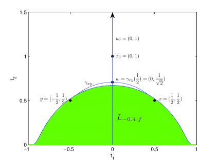
Figure 3.1

To show assertion (ii), take $z:=(2,1)$. Then

$$b_{z}=1\quad\mbox{and}\quad r_{z}=\sqrt{2}$$ (3.26)

(see (3.18)). Therefore, we have by (3.17) that $X_{0}(z)=(1,0)$. On the other hand, we get from (3.10) that

$${\rm grad}f_{0}(z)=\left(\frac{\partial f_{0}}{\partial t_{1}},\frac{\partial f_{0}}{\partial t_{2}}\right)$$

where $\frac{\partial f_{0}}{\partial t_{1}}$ and $\frac{\partial f_{0}}{\partial t_{2}}$ are classical partial derivatives in ${\mathbb{R}}^{2}$. Then, using (3.16) and (3.18), one calculates

$${\rm grad}f_{0}(z)=\left(\frac{\sqrt{2}}{8}\ln(3+2\sqrt{2})+\frac{1}{2},\frac{\sqrt{2}}{8}\ln(3+2\sqrt{2})-\frac{1}{2}\right).$$

Therefore ${\rm grad}f_{0}(z)\neq X_{0}(z)$, and assertion (ii) is checked. We further have that

$$\nabla_{\frac{\partial}{\partial t_{1}}}X_{0}(z)\neq 0.$$ (3.27)

Granting this, assertion (iii) is also checked. To show (3.27), we get from (3.9) that

$$\nabla_{\frac{\partial}{\partial t_{1}}}X_{0}=\left(\frac{\partial X_{0}^{1}}{\partial t_{1}}-\frac{1}{t_{2}}X_{0}^{2},\frac{\partial X_{0}^{2}}{\partial t_{1}}+\frac{1}{t_{2}}X_{0}^{1}\right).$$ (3.28)

(noting that ${\frac{\partial}{\partial t_{1}}}=(1,0)$ for any $x\in{\mathbb{H}}$). Recalling that $X_{0}^{1}$ and $X_{0}^{2}$ are given by (3.19) and $z:=(2,1)$, we have that $X_{0}^{1}(z)=1$ and $X_{0}^{2}(z)=0$ (noting (3.26)). Furthermore, by elemental calculus, we can calculate the partial derivatives

$$\frac{\partial X_{0}^{1}}{\partial t_{1}}\mid_{z}=0\quad\mbox{and}\quad\frac{\partial X_{0}^{2}}{\partial t_{1}}\mid_{z}=-\frac{1}{2}.$$ (3.29)

Thus we conclude from (3.28) that $\nabla_{\frac{\partial}{\partial t_{1}}}X_{0}\mid_{z}=(0,\frac{1}{2})\neq 0$, as desired to show.

For assertion (iv), we suppose on the contrary that there exists a $C^{\infty}$ function $f$ such that $X_{0}={\rm grad}f$. Then ${\rm d}\circ{\rm d}f=0$ by the fundamental property (see, e.g., [13, p. 17]). To proceed, note that $X_{0}=X_{0}^{1}\frac{\partial}{\partial t_{1}}+X_{0}^{2}\frac{\partial}{\partial t_{2}}$, where $X_{0}^{1}$ and $X_{0}^{2}$ are defined by (3.19). Then, we calculate by elementary calculus that

$$\left.\left(\frac{\partial(\frac{1}{t_{2}^{2}}X_{0}^{1})}{\partial t_{2}}-\frac{\partial(\frac{1}{t_{2}^{2}}X_{0}^{2})}{\partial t_{1}}\right)\right|_{x=(2,1)}=\frac{1}{2}\neq 0.$$ (3.30)

Furthermore, by (3.10) and (3.11), one has that

$${\rm d}f=\frac{1}{t_{2}^{2}}X_{0}^{1}{\rm d}t_{1}+\frac{1}{t_{2}^{2}}X_{0}^{2}{\rm d}t_{2},$$

and so the exterior differentiation

$${\rm d}\circ{\rm d}f=\left(\frac{\partial(\frac{1}{t_{2}^{2}}X_{0}^{2})}{\partial t_{1}}-\frac{\partial(\frac{1}{t_{2}^{2}}X_{0}^{1})}{\partial t_{2}}\right){\rm d}t_{1}\wedge{\rm d}t_{2},$$

where $\wedge$ is the exterior product; see, e.g., [13, p. 17]. This, together with (3.30), means that ${\rm d}\circ{\rm d}f\not=0$, and so assertion (iv) is shown.

4 Convexity properties of sub-level sets on Riemannian manifolds

Throughout this section, let $\kappa\in{\mathbb{R}}$ and assume that $M$ is a complete, simply connected Riemannian manifold of constant sectional curvature $\kappa$. As usual, define $D_{\kappa}:=\frac{\pi}{\sqrt{\kappa}}$ if $\kappa>0$ and $D_{\kappa}:=+\infty$ otherwise. Then, for any point $x,y\in M$ with ${\rm d}(x,y)<D_{\kappa}$, $\Gamma_{xy}$ contains a unique minimal geodesic, (which will be denoted by $\gamma_{xy}$), and any open ball ${\mathbb{B}}(x,r)$ with $r\leq\frac{D_{\kappa}}{2}$ is strongly convex for any $x\in M$; see e.g., [10, Proposition 4.1 (i)]. Let $x_{0}\in M$ and $u_{0}\in T_{x_{0}}M\setminus\{0\}$. Consider the following function $f_{0}:M\rightarrow\overline{{\mathbb{R}}}$ defined by

$$f_{0}(x)=\left\{\begin{array}[]{ll}\langle u_{0},\dot{\gamma}_{x_{0}x}(0)\rangle,&\text{ if }x\in{\mathbb{B}}(x_{0},\frac{D_{\kappa}}{2}),\\ +\infty,&\text{ otherwise},\end{array}\right.$$ (4.1)

where ${\gamma}_{x_{0}x}(0)\in{\Gamma}_{x_{0}x}$ is the unique minimal geodesic lying in ${\mathbb{B}}(x_{0},\frac{D_{\kappa}}{2})$. It is clear that ${\rm dom}f_{0}={\mathbb{B}}(x_{0},\frac{D_{\kappa}}{2})$ is strongly convex. If $M$ is a Hadamard manifold, function (4.1) is reduced to the function defined by (1.2), that is

$$f_{0}(x):=\langle u_{0},\exp_{x_{0}}^{-1}x\rangle\quad\mbox{for any $x\in M$}.$$ (4.2)

For any $c\in{\mathbb{R}}$, the sub-level set of $f_{0}$ is denoted by $L_{c,f_{0}}(c\in{\mathbb{R}})$ and defined by

$$L_{c,f_{0}}:=\{x\in M:f_{0}(x)\leq c\}.$$

Note by Example 3.1 that $L_{c,f_{0}}$ is not strongly convex in general. This section is devoted to study of the convexity property of the sub-level sets $L_{c,f_{0}}$ ($c\in{\mathbb{R}}$). For this purpose, we first recall that a geodesic triangle $\triangle(p_{1}p_{2}p_{3})$ in $M$ is a figure consisting of three points $p_{1},p_{2},p_{3}$ (the vertices of $\triangle(p_{1}p_{2}p_{3})$) and three minimal geodesic segments $\gamma_{i}$ (the edges of $\triangle(p_{1}p_{2}p_{3})$) such that $\gamma_{i}(0)=p_{i-1}$ and $\gamma_{i}(1)=p_{i+1}$ with $i=1,2,3$ ( mod$3$). For each $i=1,2,3$ ( mod$3$), the inner angle of $\triangle(p_{1}p_{2}p_{3})$ at $p_{i}$ is denoted by $\angle p_{i}$, which equals the angle between the tangent vectors $\dot{\gamma}_{i+1}(0)$ and $-\dot{\gamma}_{i-1}(1)$. The following proposition (i.e., comparison theorem for triangles) follows immediately from [13, p.161 Theorem 4.2 (ii), p. 138 Low of Cosines and p. 167 Remark 4.6].

Proposition 4.1.

Let $\triangle(p_{1}p_{2}p_{3})$ be a geodesic triangle in $M$ of the perimeter less than $2D_{\kappa}$. Set $l_{i}={\rm d}(p_{i+1},p_{i-1})$ for each $i=1,2,3$. Then, the following relations hold:

$$l_{i}^{2}<l_{i-1}^{2}+l_{i+1}^{2}-2l_{i-1}l_{i+1}\cos\angle p_{i}\quad\mbox{if $\kappa>0$},$$ (4.3)

and

$$l_{i}^{2}>l_{i-1}^{2}+l_{i+1}^{2}-2l_{i-1}l_{i+1}\cos\angle p_{i}\quad\mbox{if $\kappa<0$}.$$ (4.4)

Another property for Riemannian manifolds of constant curvature, which will be used in sequel, is the axiom of plane described as follows (see, e.g., [13, p. 136]):

Proposition 4.2.

Let $x\in M$ and let $W$ be a $k$-dimensional subspace of $T_{x}M$. Then the submanifold $N:=\exp_{x}(W\cap{\mathbb{B}}(0_{x},\rho))$ is a $k$-dimensional totally geodesic submanifold of $M$ for any $0<\rho<D_{\kappa}$. Recall a $k$-dimensional submanifold $N\subset M$ is totally geodesic iff any geodesic $\gamma$ of $M$ with the initial direction $u\in TN$ is contained in $N$; see, e.g., [13, p. 48].

The following lemma, taken from [1, Theorem 3.1 and Remark 3.6], plays a very key role in our study afterwards.

Lemma 4.1.

Let $\triangle(ypq)$ be a geodesic triangle in $M$ of the perimeter less than $2D_{\kappa}$. Let $\triangle(\tilde{y}\tilde{p}\tilde{q})$ be a triangle in ${\mathbb{R}}^{2}$ such that

$${\rm d}(y,p)=\|\overrightarrow{\tilde{y}\tilde{p}}\|,\quad{\rm d}(y,q)=\|\overrightarrow{\tilde{y}\tilde{q}}\|\quad\mbox{and}\quad\angle pyq=\angle\tilde{p}\tilde{y}\tilde{q}.$$ (4.5)

Let $x$ be in the minimal geodesic joining $p$ to $q$, and $\tilde{x}$ be the corresponding point in the interval $[\tilde{p},\tilde{q}]$ satisfying

$$\angle pyx=\angle\tilde{p}\tilde{y}\tilde{x}\quad\mbox{and}\quad\angle qyx=\angle\tilde{q}\tilde{y}\tilde{x}$$ (4.6)

(see Figure 4.1). Then, the following assertions hold:

$${\rm d}(y,x)\geq\|\overrightarrow{\tilde{y}\tilde{x}}\|\;\mbox{ if $\kappa\geq 0$}\quad\mbox{and}\quad{\rm d}(y,x)\leq\|\overrightarrow{\tilde{y}\tilde{x}}\|\;\mbox{ if $\kappa\leq 0$}.$$ (4.7)

Figure 4.1

Recall that, for any $x,y\in M$, $\gamma_{xy}\in\Gamma_{xy}$ denote the unique minimal geodesic: $\gamma_{xy}:[0,1]\to M$ is the minimal geodesic satisfying $\gamma_{xy}(0)=x$ and $\gamma_{xy}(1)=y$.

Lemma 4.2.

Let $\triangle(ypq)$ be a geodesic triangle in $M$ of the perimeter less than $2D_{\kappa}$. Let $\gamma:=\gamma_{pq}:[0,1]\rightarrow M$ be the unique minimal geodesic joining $p$ to $q$. Then, for each $t\in(0,1)$, there exist two positive numbers $a_{t}$ and $b_{t}$ satisfying

$$a_{t}+b_{t}\;\left\{\begin{array}[]{ll}\geq 1,&\mbox{if }\kappa\geq 0,\\ \leq 1,&\mbox{if }\kappa\leq 0,\\ \end{array}\right.$$ (4.8)

such that

$$\dot{\gamma}_{y\gamma(t)}(0)=a_{t}\dot{\gamma}_{yp}(0)+b_{t}\dot{\gamma}_{yq}(0).$$ (4.9)

Proof.

Since the perimeter of the geodesic triangle $\triangle(ypq)$ is less than $2D_{\kappa}$, one can verify that $\rho=\max\{\|\dot{\gamma}_{yp}(0)\|,\|\dot{\gamma}_{yq}(0)\|\}<D_{\kappa}$. Let $\rho<\bar{\rho}<D_{\kappa}$. Then, we get from Proposition 4.2 that $N:=\exp_{y}\{{\rm span}\{\dot{\gamma}_{yp}(0),\dot{\gamma}_{yq}(0)\}\cap{\mathbb{B}}(0_{y},\bar{\rho})\}$ is 2-dimensional totally geodesic sub-manifold of $M$. Hence $\gamma\subset N$ thanks to assumption. Thus, one has that

$$\dot{\gamma}_{y\gamma(t)}(0)\in T_{y}N\subseteq{\rm span}\{\dot{\gamma}_{yp}(0),\dot{\gamma}_{yq}(0)\}\quad\mbox{for any }t\in[0,1].$$ (4.10)

Thus, there exist some $a_{t},b_{t}\in{\mathbb{R}}$ such that (4.9) holds (see figure 4.1).

Below, we show that $a_{t},b_{t}$ are positive and satisfy (4.8). To this end, as in Lemma 4.1 (see Figure 1), set $x=\gamma(t)$, and let $\triangle(\tilde{y}\tilde{p}\tilde{q})$ be the corresponding triangle of $\triangle(ypq)$ in ${\mathbb{R}}^{2}$ satisfying (4.5) and $\tilde{x}$ be the corresponding point in the interval $[\tilde{p},\tilde{q}]$ satisfying (4.6). Without loss of generality, we may assume by (4.5) that $\overrightarrow{\tilde{y}\tilde{p}}=\dot{\gamma}_{yp}(0)$ and $\overrightarrow{\tilde{y}\tilde{q}}=\dot{\gamma}_{yq}(0)$. Note, by (4.10), that the vectors $\overrightarrow{\tilde{y}\tilde{x}}$ and $\dot{\gamma}_{yx}(0)$ are in the same $2$-dimensional Euclidean plane. It follows from (4.6), together with (4.9), that there exists some $\lambda>0$ such that

$$\lambda\overrightarrow{\tilde{y}\tilde{x}}=\dot{\gamma}_{yx}(0)=a_{t}\dot{\gamma}_{yp}(0)+b_{t}\dot{\gamma}_{yq}(0).$$ (4.11)

Note that $\tilde{x}$ lies actually in the open interval $(\tilde{p},\tilde{q})$ in ${\mathbb{R}}^{2}$ (as $0<t<1$ and so $\angle\tilde{p}\tilde{y}\tilde{x}>0,\;\angle\tilde{q}\tilde{y}\tilde{x}>0$ by (4.6)). It follows from (4.11) that

$$a_{t}>0,\quad b_{t}>\quad\mbox{and}\quad\frac{a_{t}+b_{t}}{\lambda}=1.$$ (4.12)

Furthermore, in view of (4.7), we see that $\lambda\leq 1$ if $\kappa\geq 0$ and $\lambda\geq 1$ if $\kappa\leq 0$. This, together with (4.12), implies that (4.8) holds and the proof is complete. ∎

Now we are ready to verify the first theorem in the present section.

Theorem 4.1.

Suppose that the constant sectional curvature $\kappa>0$ and let $f_{0}$ be the function defined by (4.1). Then the sub-level set $L_{c,f_{0}}$ is strongly convex if and only if either $c\leq 0$ or $c\geq\frac{\|u_{0}\|D_{\kappa}}{2}$.

Proof.

We first show the sufficiency part. To do this, suppose that $c\leq 0$ or $c\geq\frac{\|u_{0}\|D_{\kappa}}{2}$. Note that if $c\geq\frac{\|u_{0}\|D_{\kappa}}{2}$ then $L_{c,f_{0}}={\mathbb{B}}(x_{0},\frac{D_{\kappa}}{2})$ is strongly convex because

$$f_{0}(x)=\langle u_{0},\dot{\gamma}_{x_{0}x}(0)\rangle\leq\|u_{0}\|\cdot\|\dot{\gamma}_{x_{0}x}(0)\|\leq\frac{\|u_{0}\|D_{\kappa}}{2}\leq c.$$

holds for all $x\in{\mathbb{B}}(x_{0},\frac{D_{\kappa}}{2})$. Thus, we need only to consider the case when $c\leq 0$. To proceed, fix $c\leq 0$ and let $p,q\in L_{c,f_{0}}$, that is,

$$\langle u_{0},\dot{\gamma}_{x_{0}p}(0)\rangle\leq c\quad\mbox{and}\quad\langle u_{0},\dot{\gamma}_{x_{0}q}(0)\rangle\leq c.$$ (4.13)

Then $p,q\in{\mathbb{B}}(x_{0},\frac{D_{\kappa}}{2})$ and the geodesic triangle $\triangle(x_{0}pq)$ is well defined with perimeter less than $2D_{\kappa}$. Let $t\in[0,1]$. By assumption, Lemma 4.2 is applicable to concluding that there exist two positive numbers $a_{t}$ and $b_{t}$ satisfying with $a_{t}+b_{t}\geq 1$ such that

$$\dot{\gamma}_{x_{0}\gamma(t)}(0)=a_{t}\dot{\gamma}_{x_{0}p}(0)+b_{t}\dot{\gamma}_{x_{0}q}(0),$$

where $\gamma:=\gamma_{pq}:[0,1]\rightarrow M$ is the unique minimal geodesic joining $p$ and $q$. It follows from (4.1) and (4.13) that

$$f_{0}(\gamma(t))=a_{t}\langle u_{0},\dot{\gamma}_{x_{0}p}(0)\rangle+b_{t}\langle u_{0},\dot{\gamma}_{x_{0}q}(0)\rangle\leq c(a_{t}+b_{t})\leq c$$

(note that $c<0$). This means that $\gamma_{p,q}(t)=\gamma(t)\in L_{c,f_{0}}$ for all $t\in[0,1]$, and so $L_{c,f_{0}}$ is strongly convex as desired to show. The proof for the sufficiency part is complete.

To show the necessity part, without loss of generality, we may assume that $\|u_{0}\|=1$. Let $0<c<\frac{D_{\kappa}}{2}$. It suffices to verify that $L_{c,f_{0}}$ is not strongly convex, or equivalently, to construct two points $p,\,q$ and a number $\bar{t}\in(0,1)$ such that

$$p,q\in L_{c,f_{0}}\quad\mbox{and}\quad\bar{z}:=\gamma_{pq}(\bar{t})\notin L_{c,f_{0}}.$$ (4.14)

To do this, consider the geodesic $\gamma:[0,\frac{D_{\kappa}}{2})\to M$ defined by $\gamma(t):=\exp_{x_{0}}tu_{0}$ for each $t\in[0,\frac{D_{\kappa}}{2})$. Clearly it is contained in ${\mathbb{B}}(x_{0},\frac{D_{\kappa}}{2})$. Since ${\mathbb{B}}(x_{0},\frac{D_{\kappa}}{2})$ is strongly convex, we see that, for each $t\in[0,\frac{D_{\kappa}}{2})$, the unique minimal geodesic joining $x_{0}$ and $\gamma(t)$ can be expressed as

$$\gamma_{x_{0}\gamma(t)}(s)=\exp_{x_{0}}s(tu_{0})\quad\mbox{for each }s\in[0,1].$$

This in particular implies that, for each $t\in[0,\frac{D_{\kappa}}{2})$, $\dot{\gamma}_{x_{0}\gamma(t)}(0)=tu_{0}$ and so

$$f_{0}(\gamma(t))=\langle u_{0},\dot{\gamma}_{x_{0}\gamma(t)}(0)\rangle=\langle u_{0},tu_{0}\rangle=t.$$ (4.15)

Hence

$$\gamma(t)\in L_{c,f_{0}}\mbox{ for all }t\in[0,c]\quad\mbox{and}\quad\gamma(t)\not\in L_{c,f_{0}}\mbox{ for all }t\in(c,\frac{D_{\kappa}}{2})$$ (4.16)

because

$${\rm d}({x_{0}},z)=c<\frac{D_{\kappa}}{2},$$ (4.17)

by the choice of $c$. In particular, $z:=\gamma(c)\in L_{c,f_{0}}$. Take $u\in T_{z}M$ such that $u\perp\dot{\gamma}(c)$. Then, by (4.17), there exists some $\varepsilon>0$ such that the geodesic $\tau:[-\varepsilon,\varepsilon]\rightarrow M$, determined by $\tau(0)=z$ and $\dot{\tau}(0)=u$, is contained in ${\mathbb{B}}(x_{0},\frac{D_{\kappa}}{2})\cap{\mathbb{B}}(z,\frac{D_{\kappa}}{2})$. Set $p_{\varepsilon}:=\tau(\varepsilon)$ and $q_{\varepsilon}:=\tau(-\varepsilon)$ (see, Figure 4.2). Then

$$p_{\varepsilon},\;q_{\varepsilon}\in{\mathbb{B}}(x_{0},\frac{D_{\kappa}}{2})\cap{\mathbb{B}}(z,\frac{D_{\kappa}}{2}).$$ (4.18)

Below, we shall show that

$$p_{\varepsilon},\;q_{\varepsilon}\in L_{c,f_{0}}\mbox{ with $f_{0}(p_{\varepsilon})<c$ and $f_{0}(q_{\varepsilon})<c$}.$$ (4.19)

Consider the geodesic triangle $\triangle(x_{0}zp_{\varepsilon})$. Then its perimeter is less than $2D_{\kappa}$ thanks to (4.17) and (4.18). Thus Proposition 4.1 is applicable, and using (4.4), we have that

$${\rm d}^{2}(x_{0},p_{\varepsilon})<{\rm d}^{2}(x_{0},z)+{\rm d}^{2}(z,p_{\varepsilon})-2{\rm d}(x_{0},z){\rm d}(z,p_{\varepsilon})\cos\angle p_{\varepsilon}zx_{0}={\rm d}^{2}(x_{0},z)+{\rm d}^{2}(z,p_{\varepsilon}),$$

(noting that $\angle p_{\varepsilon}zx_{0}=\frac{\pi}{2}$ as $\dot{\tau}(0)\perp\dot{\gamma}(c)$), and

$${\rm d}^{2}(z,p_{\varepsilon})<{\rm d}^{2}(x_{0},z)+{\rm d}^{2}(x_{0},p_{\varepsilon})-2{\rm d}(x_{0},z){\rm d}(x_{0},p_{\varepsilon})\cos\angle p_{\varepsilon}x_{0}z.$$

Combining these two inequalities, we get that

$${\rm d}(x_{0},p_{\varepsilon})\cos\angle p_{\varepsilon}x_{0}z<{\rm d}(x_{0},z).$$

Thus

$$f_{0}(p_{\varepsilon})={\rm d}(x_{0},p_{\varepsilon})\cdot\|u_{0}\|\cdot\cos\angle p_{\varepsilon}x_{0}z={\rm d}(x_{0},p_{\varepsilon})\cos\angle p_{\varepsilon}x_{0}z<{\rm d}(x_{0},z)=c,$$

where the last equality holds because of (4.17). Similarly, we have $f_{0}(q_{\varepsilon})<c$ and (4.19) is shown.

Let $\gamma_{x_{0}}:[0,\infty)\rightarrow M$ be the geodesic satisfying that $\gamma_{x_{0}}(0)=x_{0}$ and $\gamma_{x_{0}}(1)=p_{\varepsilon}$. In light of (4.18) and (4.19), we get by the continuity of $f_{0}$ that there exists $t_{0}>1$ such that $\gamma_{x_{0}}(t_{0})\in L_{c,f_{0}}$. Set $p:=\gamma_{x_{0}}(t_{0})$ and $q:=q_{\varepsilon}$. Then, $p,\;q\in L_{c,f_{0}}$ (see (4.19)). We further show that

$$\bar{z}:=\gamma_{pq}(\bar{t})\notin L_{c,f_{0}}\;\mbox{ for some }\bar{t}\in(0,1).$$ (4.20)

Granting this, (4.14) is established. To show (4.20), write $\widetilde{N}:=\exp_{z}\{{\rm span}\{\dot{\gamma}_{zx_{0}}(0),u\}\cap{\mathbb{B}}(0_{z},\frac{D_{\kappa}}{2})\}$. Then $\widetilde{N}$ is a 2-dimensional totally geodesic sub-manifold of $M$ by Proposition 4.2 (recalling that $M$ is of constant curvature). Since points $x_{0},p,q,p_{\varepsilon},z$ lie in $\widetilde{N}$, it follows that $\gamma_{pq}$ must meet $\gamma$ at some point $\bar{z}:=\gamma_{pq}(\bar{t})=\gamma(c_{0})$ with $\bar{t}\in(0,1)$ and $c_{0}>c$ (see Figure 4.2). In light of (4.16), one sees that $\bar{z}\not\in L_{c,f_{0}}$. Thus (4.20) is shown, and the proof is complete. ∎

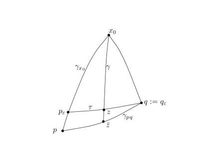
Figure 4.2

Our second theorem in this section is Theorem 4.2 below, which is an analogue of Theorem 4.1 on Hadamard manifold of constant sectional curvature. In particular, Theorem 4.2 improves and extends the corresponding result in [6, Corollary 3.1], where it was shown that the sub-level sets $L_{c,f_{0}}$ is convex in the special case when $c=0$. The proof of Theorem 4.2 is quite similar to that we did for Theorem 4.1 and so we omit it here.

Theorem 4.2.

Suppose that the constant sectional curvature $\kappa<0$ and let $f_{0}$ be the function defined by (4.2). Then, $L_{c,f_{0}}$ is convex if and only if $c\geq 0$.

As a direct consequence of Theorems 4.1 and 4.2, together with Proposition 2.2, we have the following corollary which shows that the function defined by (4.1) is not quasi-convex in general.

Corollary 4.1.

Suppose that $M$ is of non-zero constant sectional curvature. Let $x_{0}\in M$ and $u_{0}\in T_{x_{0}}M\setminus\{0\}$. Then, the functions defined by (4.1) is not quasi-convex.

References

- [1] Afsari, B., Tron, R., Vidal, R.: On the convergence of gradient descent for finding the Riemannian center of mass. SIAM J. Control Optim. 51(3), 2230–2260 (2013)
- [2] Cheeger, J., Gromoll, D., On the structure of complete manifolds of nonnegative curvature, Ann. Math. 96, 413–443(1972).
- [3] Colao, V., López, G., Marino, G., Martín-Márquez, V.: Equilibrium problems in Hadamard manifolds. J. Math. Anal. Appl. 388(1), 61–77 (2012)
- [4] do Carmo, M.P.: Riemannian Geometry. Birkhäuser Boston, Boston MA (1992)
- [5] Eisenhard, L.P.: Riemannian Geometry. Princeton University, Princeton, N. J. (1925)
- [6] Ferreira, O.P., lucambio Pérez, L.R., Németh, S.Z.: Singularities of monotone vector fields and an extragradient-type algorithm. J. Global Optim. 31, 133–151 (2005)
- [7] Kristál, A., Li, C, Lopez, G., Nicolae, A.: What do “convexities” imply on Hadamard manifolds?. to appear in J. Optim. Theory Appl.
- [8] Li, S.L, Li, C., Yao, J.C.: Existence of solutions for variational inequalities on Riemannian manifolds. Nonlinear Anal. 71, 5695–5706(2009).
- [9] Li, C., Mordukhovich, B.S., Wang, J., Yao, J.C.: Weak sharp minima on Riemannian manifolds. SIAM J. Optim. 21, 1523–1560(2011).
- [10] Li, C., Yao, J.C.: Variational inequalities for set-valued vector fields on Riemannian manifolds: convexity of the solution set and the proximal point algorithm. SIAM J. Control Optim. 50(4), 2486–2514 (2012)
- [11] Papa Quiroz, E.A., Oliveira, P.R.: Proximal point methods for quasiconvex and convex functions with Bregman distances on Hadamard manifolds. J. Convex Anal. 16(1), 49–69 (2009)
- [12] Papa Quiroz, E.A.: An extension of the proximal point algorithm with Bregman distances on Hadamard manifolds. J. Global Optim. 56(1), 43–59 (2013)
- [13] Sakai, T.: Riemannian Geometry. Trans. Math. Monogr. 149. American Mathematical Society, Providence RI (1996)
- [14] Udriste, C.: Convex Functions and Optimization Methods on Riemannian Manifolds. In: Mathematics and Its Applications 297. Kluwer Academic, Dordrecht (1994)
- [15] Walter, R.: On the metric projection onto convex sets in Riemannian spaces. Arch. Math., 25, 91–98(1974).
- [16] Wang, J. H, López, G., Martín-Márquez, V., Li, C.: Monotone and Accretive Vector Fields on Riemannian Manifolds. J. Optim. Theory Appl., 146, 691–708(2010).
- [17] Wang, X. M., Li, C., Yao, J. C.: Projection algorithms for solving convex feasibility problems on Hadamard manifolds. to appear in J. Nonlin. Convex Appl.
- [18] Yau, S.T.: Non-existence of continuous convex functions on certain Riemannian manifolds. Math. Ann. 207, 269–270 (1974)
- [19] Zhou, L., Huang, N.: Existence of solutions for vector optimization on Hadamard manifolds. J. Optim. Theory Appl. 157(1), 44–53 (2013)