Optimal-observable analysis of possible new physics in BD()τντ𝐵superscript𝐷𝜏subscript𝜈𝜏B\to D^{(\ast)}\tau\nu_{\tau}

Srimoy Bhattacharya Indian Institute of Technology, North Guwahati, Guwahati 781039, Assam, India    Soumitra Nandi Indian Institute of Technology, North Guwahati, Guwahati 781039, Assam, India    Sunando Kumar Patra Indian Institute of Technology, North Guwahati, Guwahati 781039, Assam, India
Abstract

We study all possible observables in BD()τντ𝐵superscript𝐷𝜏subscript𝜈𝜏B\to D^{(\ast)}\tau\nu_{\tau} with new physics (NP), including new vector, scalar and tensor interactions, and investigate the prospects of extracting NP Wilson coefficients with optimal observables. Analysis of the full q2superscript𝑞2q^{2} integrated branching fractions of BD()τντ𝐵superscript𝐷𝜏subscript𝜈𝜏B\to D^{(\ast)}\tau\nu_{\tau} show that the overall sensitivity of the observables of BDτντ𝐵𝐷𝜏subscript𝜈𝜏B\to D\tau\nu_{\tau} is more towards the scalar current, whereas the bin-by-bin analysis of q2superscript𝑞2q^{2} distribution of the differential branching fraction points to regions of q2superscript𝑞2q^{2} sensitive to tensor interactions. Interestingly, the observables in BDτντ𝐵superscript𝐷𝜏subscript𝜈𝜏B\to D^{\ast}\tau\nu_{\tau} are more sensitive to tensor interactions, and bin-by-bin analysis of this mode shows the distinct regions of q2superscript𝑞2q^{2} sensitive to vector or scalar interactions. In addition to that, the τ𝜏\tau polarisation asymmetry is found to be more sensitive to NP compared to the other observables, in both decay modes.

I Introduction

Measurements of branching fractions and other related observables in semileptonic decays of B𝐵B meson to τ𝜏\tau can be interesting for an indirect probe of NP. Earlier measurements on R(D())=(BD()τντ)/(BD()ν)𝑅superscript𝐷𝐵superscript𝐷𝜏subscript𝜈𝜏𝐵superscript𝐷subscript𝜈R(D^{(\ast)})={{\cal BR}{(B\to D^{(\ast)}\tau\nu_{\tau})}}/{{\cal BR}{(B\to D^{(\ast)}\ell\nu_{\ell})}} by Belle Adachi:2009qg and BABAR collaborations Lees:2013uzd have shown some deviations from their Standard Model(SM) predictions Fajfer:2012vx , indicating a possible signature of NP in bcτντ𝑏𝑐𝜏subscript𝜈𝜏b\to c\tau\nu_{\tau} transitions. Several authors have tried to explain the observation in various NP scenarios Tanaka:1994 ; Sakaki:2013 ; Duraisamy:2014 , as well as in a model-independent way Tanaka:2012 ; Sakaki:2014 ; Freytsis:2015 . In order to distinguish between the possible signatures of NP, the study of NP in q2superscript𝑞2q^{2} distribution of differential branching fractions in BD()τντ𝐵superscript𝐷𝜏subscript𝜈𝜏B\to D^{(\ast)}\tau\nu_{\tau}, various correlations among τ𝜏\tau forward-backward asymmetry and τ𝜏\tau polarization asymmetry has been examined in the Ref. Fajfer:2012 ; Sakaki:2013 ; Biancofiore:2013 . Recently, a 2.1σ𝜎\sigma deviation in the measurement of R(D)𝑅superscript𝐷R(D^{\ast}) has been reported by LHCb collaboration Aaij:2015yra ; Belle collaboration has also announced their most recent results on R(D())𝑅superscript𝐷R(D^{(\ast)}) and measured values are consistent with the SM within error bars Huschle:2015 .

So far, the constraints on the new couplings are obtained assuming their presence one at a time Sakaki:2013 ; Sakaki:2014 . If we consider all the interactions together, then it will be an impossible task to extract all the couplings from a single measurement. However, if one can reduce the number of coupling parameters by imposing certain constraints on the full set of parameters, only then it is possible to obtain meaningful errors on the couplings, although the information lost due to various assumptions cannot be retrieved. Therefore, it will be useful to have independent couplings, parametrised in such a way that the measured errors on different parameters are uncorrelated. On the other hand, it is not necessary for a particular observable to have equal sensitivity to different types of NP operators. Therefore, it is useful to know how an observable can be optimised to guarantee the maximal sensitivity to a particular type of NP interaction, which in turn will help us select observables suitable for the extraction of a particular type of coupling. Hence, from a phenomenological point of view, it is important to find out the significance of different types of NP interaction, to an observable. To achieve this goal, we use the optimal-observable analysis using the invariant mass squared q2superscript𝑞2q^{2}, of the lepton-neutrino system. We construct the optimal observable to identify the NP structure that can be best extracted from a particular observable, with reasonable statistics. It also provides a deeper understanding of the sensitivity that can be best obtained by any method, for a certain process. This technique has been widely used in collider phenomenology davier93 ; Diehl:1993br ; Atwood:1991ka ; Gunion:1996 ; Diehl:1997 ; wudka2004 .

In this article, we analyse the q2superscript𝑞2q^{2} distribution of the differential branching fractions, R(D())𝑅superscript𝐷R(D^{(\ast)}), the τ𝜏\tau polarisation asymmetries, forward backward asymmetries of the decay BD()τντ𝐵superscript𝐷𝜏subscript𝜈𝜏B\to D^{(\ast)}\tau\nu_{\tau}, and Dsuperscript𝐷D^{*} polarisation asymmetry. We include all possible non-standard four-fermi effective interactions of the lowest dimension, and estimate the expected statistical uncertainties in the extraction of various NP Wilson coefficients that can contribute to BD()τντ𝐵superscript𝐷𝜏subscript𝜈𝜏B\to D^{(\ast)}\tau\nu_{\tau}.

II Methodology

The most general effective Hamiltonian describing the bcτντ𝑏𝑐𝜏subscript𝜈𝜏b\to c\tau\nu_{\tau} transitions with all possible four-fermi operators in the lowest dimension is given by Sakaki:2014

effsubscript𝑒𝑓𝑓\displaystyle{\cal H}_{eff} =4GF2Vcb[(1+CV1)𝒪V1+CV2𝒪V2\displaystyle=\frac{4G_{F}}{\sqrt{2}}V_{cb}\Big{[}(1+C_{V_{1}}){\cal O}_{V_{1}}+C_{V_{2}}{\cal O}_{V_{2}}
+CS1𝒪S1+CS2𝒪S2+CT𝒪T],\displaystyle+C_{S_{1}}{\cal O}_{S_{1}}+C_{S_{2}}{\cal O}_{S_{2}}+C_{T}{\cal O}_{T}\Big{]}, (1)

where the operator basis is defined as

𝒪V1subscript𝒪subscript𝑉1\displaystyle{\cal O}_{V_{1}} =\displaystyle= (c¯LγμbL)(τ¯LγμντL),𝒪V2=(c¯RγμbR)(τ¯LγμντL),subscript¯𝑐𝐿superscript𝛾𝜇subscript𝑏𝐿subscript¯𝜏𝐿subscript𝛾𝜇subscript𝜈𝜏𝐿subscript𝒪subscript𝑉2subscript¯𝑐𝑅superscript𝛾𝜇subscript𝑏𝑅subscript¯𝜏𝐿subscript𝛾𝜇subscript𝜈𝜏𝐿\displaystyle({\bar{c}}_{L}\gamma^{\mu}b_{L})({\bar{\tau}}_{L}\gamma_{\mu}\nu_{\tau L}),~{}{\cal O}_{V_{2}}=({\bar{c}}_{R}\gamma^{\mu}b_{R})({\bar{\tau}}_{L}\gamma_{\mu}\nu_{\tau L}),
𝒪S1subscript𝒪subscript𝑆1\displaystyle{\cal O}_{S_{1}} =\displaystyle= (c¯LbR)(τ¯RντL),𝒪S2=(c¯RbL)(τ¯RντL),subscript¯𝑐𝐿subscript𝑏𝑅subscript¯𝜏𝑅subscript𝜈𝜏𝐿subscript𝒪subscript𝑆2subscript¯𝑐𝑅subscript𝑏𝐿subscript¯𝜏𝑅subscript𝜈𝜏𝐿\displaystyle({\bar{c}}_{L}b_{R})({\bar{\tau}}_{R}\nu_{\tau L}),~{}~{}~{}~{}~{}~{}~{}~{}{\cal O}_{S_{2}}=({\bar{c}}_{R}b_{L})({\bar{\tau}}_{R}\nu_{\tau L}),
𝒪Tsubscript𝒪𝑇\displaystyle{\cal O}_{T} =\displaystyle= (c¯RσμνbL)(τ¯RσμνντL),subscript¯𝑐𝑅superscript𝜎𝜇𝜈subscript𝑏𝐿subscript¯𝜏𝑅subscript𝜎𝜇𝜈subscript𝜈𝜏𝐿\displaystyle({\bar{c}}_{R}\sigma^{\mu\nu}b_{L})({\bar{\tau}}_{R}\sigma_{\mu\nu}\nu_{\tau L}), (2)

and the corresponding Wilson coefficients are given by CW(W=V1,V2,S1,S2,T)subscript𝐶𝑊𝑊subscript𝑉1subscript𝑉2subscript𝑆1subscript𝑆2𝑇C_{W}(W=V_{1},V_{2},S_{1},S_{2},T). In this basis, neutrinos are assumed to be left handed. Our main focus is on the q2superscript𝑞2q^{2} distribution of differential decay rate dΓ/dq2𝑑Γ𝑑superscript𝑞2d\Gamma/dq^{2} in BD()τντ𝐵superscript𝐷𝜏subscript𝜈𝜏B\to D^{(\ast)}\tau\nu_{\tau}. The complete expressions are given in ref.Sakaki:2013 .

As mentioned earlier, the optimal-observable analysis is a technique to systematically estimate the statistical uncertainties of the measurable parameters while extracting them from some observable. Elaborate discussions on this technique can be found in references Diehl:1993br ; Atwood:1991ka ; Gunion:1996 ; Diehl:1997 . In order to apply this technique to BD()τντ𝐵superscript𝐷𝜏subscript𝜈𝜏B\to D^{(\ast)}\tau\nu_{\tau}, it is necessary to express the q2superscript𝑞2q^{2} distribution of the differential decay rate as

dΓ(BD()τντ)dq2=iCifi(q2),𝑑Γ𝐵superscript𝐷𝜏subscript𝜈𝜏𝑑superscript𝑞2subscript𝑖subscript𝐶𝑖subscript𝑓𝑖superscript𝑞2\frac{d{\Gamma}(B\to D^{(\ast)}\tau\nu_{\tau})}{dq^{2}}=\sum\limits_{i}C_{i}f_{i}(q^{2}), (3)

where Cisubscript𝐶𝑖C_{i}s are functions of CWsubscript𝐶𝑊C_{W}s. The theoretical expressions for Cisubscript𝐶𝑖C_{i}s, along with the fi(q2)subscript𝑓𝑖superscript𝑞2f_{i}(q^{2})s, can be extracted from a direct comparison between the similar terms on both sides of eq.(3). The coefficients Cisubscript𝐶𝑖C_{i}, relevant for the branching fractions in BD()τντ𝐵superscript𝐷𝜏subscript𝜈𝜏B\to D^{(\ast)}\tau\nu_{\tau}, are given in Table 1, and the corresponding fi(q2)subscript𝑓𝑖superscript𝑞2f_{i}(q^{2})s are given in the Appendix (Table 14).

Cisubscript𝐶𝑖C_{i} Obs d/dq2𝑑𝑑superscript𝑞2d{\cal B}/{dq^{2}} in BDτντ𝐵𝐷𝜏subscript𝜈𝜏B\to D\tau\nu_{\tau} d/dq2𝑑𝑑superscript𝑞2d{\cal B}/{dq^{2}} in BDτντ𝐵superscript𝐷𝜏subscript𝜈𝜏B\to D^{\ast}\tau\nu_{\tau}
C1subscript𝐶1C_{1} |1+CV1+CV2|2superscript1subscript𝐶subscript𝑉1subscript𝐶subscript𝑉22|1+C_{V_{1}}+C_{V_{2}}|^{2} |1+CV1|2+|CV2|2superscript1subscript𝐶subscript𝑉12superscriptsubscript𝐶subscript𝑉22|1+C_{V_{1}}|^{2}+|C_{V_{2}}|^{2}
C2subscript𝐶2C_{2} |CS1+CS2|2superscriptsubscript𝐶subscript𝑆1subscript𝐶subscript𝑆22|C_{S_{1}}+C_{S_{2}}|^{2} Re[(1+CV1)CV2]𝑅𝑒delimited-[]1subscript𝐶subscript𝑉1superscriptsubscript𝐶subscript𝑉2Re[(1+C_{V_{1}})C_{V_{2}}^{\ast}]
C3subscript𝐶3C_{3} |CT|2superscriptsubscript𝐶𝑇2|C_{T}|^{2} |CS1CS2|2superscriptsubscript𝐶subscript𝑆1subscript𝐶subscript𝑆22|C_{S_{1}}-C_{S_{2}}|^{2}
C4subscript𝐶4C_{4} Re[(1+CV1+CV2)(CS1+CS2)]𝑅𝑒delimited-[]1subscript𝐶subscript𝑉1subscript𝐶subscript𝑉2superscriptsubscript𝐶subscript𝑆1superscriptsubscript𝐶subscript𝑆2Re[(1+C_{V_{1}}+C_{V_{2}})(C_{S_{1}}^{\ast}+C_{S_{2}}^{\ast})] |CT|2superscriptsubscript𝐶𝑇2|C_{T}|^{2}
C5subscript𝐶5C_{5} Re[(1+CV1+CV2)CT]𝑅𝑒delimited-[]1subscript𝐶subscript𝑉1subscript𝐶subscript𝑉2superscriptsubscript𝐶𝑇Re[(1+C_{V_{1}}+C_{V_{2}})C_{T}^{\ast}] Re[(1+CV1CV2)(CS1CS2)]𝑅𝑒delimited-[]1subscript𝐶subscript𝑉1subscript𝐶subscript𝑉2superscriptsubscript𝐶subscript𝑆1superscriptsubscript𝐶subscript𝑆2Re[(1+C_{V_{1}}-C_{V_{2}})(C_{S_{1}}^{\ast}-C_{S_{2}}^{\ast})]
C6subscript𝐶6C_{6} Re[(1+CV1)CT]𝑅𝑒delimited-[]1subscript𝐶subscript𝑉1superscriptsubscript𝐶𝑇Re[(1+C_{V_{1}})C_{T}^{\ast}]
C7subscript𝐶7C_{7} Re[CV2CT]𝑅𝑒delimited-[]subscript𝐶subscript𝑉2superscriptsubscript𝐶𝑇Re[C_{V_{2}}C_{T}^{\ast}]
Table 1: Cisubscript𝐶𝑖C_{i}s as defined in eq.(3). The observable PτR(q2)subscriptsuperscript𝑃𝑅𝜏superscript𝑞2P^{R}_{\tau}(q^{2}) contains the same set of Cisubscript𝐶𝑖C_{i}s.

The goal of this technique is to extract Cisubscript𝐶𝑖C_{i}s, which can be done by defining suitable weighting functions wi(q2)subscript𝑤𝑖superscript𝑞2w_{i}(q^{2}) such as Ci=wi(q2)(dΓ/dq2)𝑑q2subscript𝐶𝑖subscript𝑤𝑖superscript𝑞2𝑑Γ𝑑superscript𝑞2differential-dsuperscript𝑞2C_{i}=\int w_{i}(q^{2})({d\Gamma}/{dq^{2}})dq^{2}. In general various choices of wisubscript𝑤𝑖w_{i}s are possible. However, there is a unique choice for which the resulting error in the extraction of Cisubscript𝐶𝑖C_{i} is minimized 111Cisubscript𝐶𝑖C_{i}s are minimised in a sense that the whole covariance matrix is at a stationary point in terms of varying the functional forms of wi(q2)subscript𝑤𝑖superscript𝑞2w_{i}(q^{2}) while maintaining wi(q2)fk(q2)=δiksubscript𝑤𝑖superscript𝑞2subscript𝑓𝑘superscript𝑞2subscript𝛿𝑖𝑘\int{w_{i}(q^{2})f_{k}(q^{2})}=\delta_{ik}., and these functions are given by

wi(q2)=jXijfj(q2)dΓ/dq2,subscript𝑤𝑖superscript𝑞2subscript𝑗subscript𝑋𝑖𝑗subscript𝑓𝑗superscript𝑞2𝑑Γ𝑑superscript𝑞2w_{i}(q^{2})=\sum_{j}\frac{X_{ij}f_{j}(q^{2})}{d{\Gamma}/{dq^{2}}}, (4)

where Xijsubscript𝑋𝑖𝑗X_{ij} is the inverse of Mijsubscript𝑀𝑖𝑗M_{ij} which is defined as

Mij=𝑑q2fi(q2)fj(q2)fSM(q2).subscript𝑀𝑖𝑗differential-dsuperscript𝑞2subscript𝑓𝑖superscript𝑞2subscript𝑓𝑗superscript𝑞2subscript𝑓𝑆𝑀superscript𝑞2M_{ij}=\int dq^{2}\frac{f_{i}(q^{2})f_{j}(q^{2})}{f_{SM}(q^{2})}. (5)

In the above expression, fSM(q2)subscript𝑓𝑆𝑀superscript𝑞2f_{SM}(q^{2}) can be obtained from eq.(3) by setting CW=0subscript𝐶𝑊0C_{W}=0, while CSM=1subscript𝐶𝑆𝑀1C_{SM}=1. Hence, using eqs. (4), and (5) the statistical uncertainties in Cisubscript𝐶𝑖C_{i} extracted from the branching fractions can be obtained as Atwood:1991ka ; Gunion:1996

|δCi|=Xii(BD()τντ)expNsig=XiiσPeff,𝛿subscript𝐶𝑖subscript𝑋𝑖𝑖superscript𝐵superscript𝐷𝜏subscript𝜈𝜏𝑒𝑥𝑝subscript𝑁𝑠𝑖𝑔subscript𝑋𝑖𝑖subscript𝜎𝑃subscript𝑒𝑓𝑓|\delta C_{i}|=\sqrt{\frac{X_{ii}{{\cal B}(B\to D^{(\ast)}\tau\nu_{\tau})}^{exp}}{N_{sig}}}=\sqrt{\frac{X_{ii}}{\sigma_{P}{\cal L}_{eff}}}, (6)

where exp=(1/Γ)𝑑q2𝑑Γ/𝑑q2superscript𝑒𝑥𝑝1Γdifferential-dsuperscript𝑞2differential-dΓdifferential-dsuperscript𝑞2{\cal B}^{exp}=(1/\Gamma)\int dq^{2}d\Gamma/dq^{2} is the total branching fraction in the decay BD()τντ𝐵superscript𝐷𝜏subscript𝜈𝜏B\to D^{(\ast)}\tau\nu_{\tau} with ΓΓ\Gamma as the total decay width. Nsigsubscript𝑁𝑠𝑖𝑔N_{sig} is the total number of events. As given in eq.(6), the errors are also related to the production cross section σPsubscript𝜎𝑃\sigma_{P} ( = σBD()τντ/(BD()τντ)subscript𝜎𝐵superscript𝐷𝜏subscript𝜈𝜏𝐵superscript𝐷𝜏subscript𝜈𝜏\sigma_{B\to D^{(\ast)}\tau\nu_{\tau}}/{\cal B}(B\to D^{(\ast)}\tau\nu_{\tau})), and the effective luminosity eff=intϵssubscript𝑒𝑓𝑓subscript𝑖𝑛𝑡subscriptitalic-ϵ𝑠{\cal L}_{eff}={\cal L}_{int}\epsilon_{s}, where intsubscript𝑖𝑛𝑡{\cal L}_{int} and ϵssubscriptitalic-ϵ𝑠\epsilon_{s} are the integrated luminosity and reconstruction efficiency respectively 222As we know that the cross section σab=σaΓb/Γsubscript𝜎𝑎𝑏subscript𝜎𝑎subscriptΓ𝑏Γ\sigma_{a\to b}=\sigma_{a}\Gamma_{b}/\Gamma, therefore, we can define σBD()τντ=σP(BD()τντ)subscript𝜎𝐵superscript𝐷𝜏subscript𝜈𝜏subscript𝜎𝑃𝐵superscript𝐷𝜏subscript𝜈𝜏\sigma_{B\to D^{(\ast)}\tau\nu_{\tau}}=\sigma_{P}{\cal B}(B\to D^{(\ast)}\tau\nu_{\tau}), where σPsubscript𝜎𝑃\sigma_{P} is the BB¯𝐵¯𝐵B{\bar{B}} production cross section. If we redefine our observable as σBD()τντsubscript𝜎𝐵superscript𝐷𝜏subscript𝜈𝜏\sigma_{B\to D^{(\ast)}\tau\nu_{\tau}} than the errors in Cisubscript𝐶𝑖C_{i} can be written as δCi𝛿subscript𝐶𝑖\displaystyle\delta C_{i} =\displaystyle= XiiσBD()τντNsig=Xiieff=XiiσPeffsuperscriptsubscript𝑋𝑖𝑖subscript𝜎𝐵superscript𝐷𝜏subscript𝜈𝜏subscript𝑁𝑠𝑖𝑔superscriptsubscript𝑋𝑖𝑖subscript𝑒𝑓𝑓subscript𝑋𝑖𝑖subscript𝜎𝑃subscript𝑒𝑓𝑓\displaystyle\sqrt{\frac{X_{ii}^{\prime}\sigma_{B\to D^{(\ast)}\tau\nu_{\tau}}}{N_{sig}}}=\sqrt{\frac{X_{ii}^{\prime}}{{\cal L}_{eff}}}=\sqrt{\frac{X_{ii}}{\sigma_{P}{\cal L}_{eff}}} =\displaystyle= Xii(BD()τντ)expNsig,subscript𝑋𝑖𝑖superscript𝐵superscript𝐷𝜏subscript𝜈𝜏𝑒𝑥𝑝subscript𝑁𝑠𝑖𝑔\displaystyle\sqrt{\frac{X_{ii}{{\cal B}(B\to D^{(\ast)}\tau\nu_{\tau})}^{exp}}{N_{sig}}}, since Xii=Xii/σPsuperscriptsubscript𝑋𝑖𝑖subscript𝑋𝑖𝑖subscript𝜎𝑃X_{ii}^{\prime}=X_{ii}/\sigma_{P}. . The above-mentioned method, and the equations like (5) and (6), can be generalised for any other observables in BD()τντ𝐵superscript𝐷𝜏subscript𝜈𝜏B\to D^{(\ast)}\tau\nu_{\tau} decay.

Since the data is consistent with the SM, if there is NP in BD()τντ𝐵superscript𝐷𝜏subscript𝜈𝜏B\to D^{(\ast)}\tau\nu_{\tau} decays, the effect is expected to be small compared to their SM counterpart. The earlier model independent analysis Sakaki:2014 , which is based on data by BABAR Lees:2013uzd , shows that zero value of the new Wilson coefficients are consistent with the data. Therefore, we choose our starting point as CW=0subscript𝐶𝑊0C_{W}=0 and find out errors in the extraction of those coefficients around that point. In addition to that, we assume that the error on Cisubscript𝐶𝑖C_{i} could be captured sufficiently well by just the leading-order terms.

We focus on the following observables:

  • The branching fractions, obtained by integrating the differential branching fractions over the full q2superscript𝑞2q^{2} region, normalised by the full q2superscript𝑞2q^{2} integrated branching fraction =(BD()ν)subscript𝐵superscript𝐷subscript𝜈{\cal B}_{\ell}={\cal B}(B\to D^{(\ast)}\ell\nu_{\ell}).

    R(D())=𝑑q2RD()(q2),𝑅superscript𝐷differential-dsuperscript𝑞2subscript𝑅superscript𝐷superscript𝑞2R(D^{(\ast)})=\int dq^{2}R_{D^{(\ast)}}(q^{2}), (7)

    with

    RD()(q2)=1d(BD()τντ)dq2.subscript𝑅superscript𝐷superscript𝑞21subscript𝑑𝐵superscript𝐷𝜏subscript𝜈𝜏𝑑superscript𝑞2R_{D^{(\ast)}}(q^{2})=\frac{1}{{\cal B}_{\ell}}\frac{d{\cal B}(B\to D^{(\ast)}\tau\nu_{\tau})}{dq^{2}}. (8)
  • τ𝜏\tau polarisation asymmetry which we defined as PτR()(q2)=Pτ(q2)RD()(q2)superscriptsubscript𝑃𝜏superscript𝑅superscript𝑞2subscript𝑃𝜏superscript𝑞2subscript𝑅superscript𝐷superscript𝑞2P_{\tau}^{R^{(*)}}(q^{2})=P_{\tau}(q^{2})R_{D^{(\ast)}}(q^{2}), where

    Pτ(q2)=dΓλ=1/2/dq2dΓλ=1/2/dq2dΓλ=1/2/dq2+dΓλ=1/2/dq2.subscript𝑃𝜏superscript𝑞2𝑑subscriptΓ𝜆12𝑑superscript𝑞2𝑑subscriptΓ𝜆12𝑑superscript𝑞2𝑑subscriptΓ𝜆12𝑑superscript𝑞2𝑑subscriptΓ𝜆12𝑑superscript𝑞2P_{\tau}(q^{2})=\frac{d\Gamma_{\lambda=1/2}/dq^{2}-d\Gamma_{\lambda=-1/2}/dq^{2}}{d\Gamma_{\lambda=1/2}/dq^{2}+d\Gamma_{\lambda=-1/2}/dq^{2}}. (9)
  • τ𝜏\tau forward-backward asymmetry 𝒜FBR()(q2)=𝒜FB(q2)RD()(q2)superscriptsubscript𝒜𝐹𝐵superscript𝑅superscript𝑞2subscript𝒜𝐹𝐵superscript𝑞2subscript𝑅superscript𝐷superscript𝑞2{\cal A}_{FB}^{R^{(*)}}(q^{2})={\cal A}_{FB}(q^{2})R_{D^{(\ast)}}(q^{2}), where

    𝒜FB(q2)subscript𝒜𝐹𝐵superscript𝑞2\displaystyle{\cal A}_{FB}(q^{2}) =\displaystyle= 01dΓdq2dcosθdcosθ10dΓdq2dcosθdcosθ11dΓdq2dcosθdcosθsuperscriptsubscript01𝑑Γ𝑑superscript𝑞2𝑑𝜃𝑑𝜃superscriptsubscript10𝑑Γ𝑑superscript𝑞2𝑑𝜃𝑑𝜃superscriptsubscript11𝑑Γ𝑑superscript𝑞2𝑑𝜃𝑑𝜃\displaystyle\frac{\int_{0}^{1}\frac{d\Gamma}{dq^{2}d\cos\theta}d\cos\theta-\int_{-1}^{0}\frac{d\Gamma}{dq^{2}d\cos\theta}d\cos\theta}{\int_{-1}^{1}\frac{d\Gamma}{dq^{2}d\cos\theta}d\cos\theta} (10)
    =\displaystyle= bθ(q2)dΓ/dq2,subscript𝑏𝜃superscript𝑞2𝑑Γ𝑑superscript𝑞2\displaystyle\frac{b_{\theta}(q^{2})}{d\Gamma/dq^{2}},

    where θ𝜃\theta is the angle that τ𝜏\tau makes with the B¯¯𝐵\bar{B} in the rest frame of τν¯𝜏¯𝜈\tau{\bar{\nu}}. The expressions for bθ(q2)subscript𝑏𝜃superscript𝑞2b_{\theta}(q^{2}) are given in Sakaki:2013 .

  • Dsuperscript𝐷D^{\ast} longitudinal polarisation asymmetry PDR(q2)=PD(q2)RD(q2)superscriptsubscript𝑃superscript𝐷𝑅superscript𝑞2subscript𝑃superscript𝐷superscript𝑞2subscript𝑅superscript𝐷superscript𝑞2P_{D^{\ast}}^{R}(q^{2})=P_{D^{\ast}}(q^{2})R_{D^{\ast}}(q^{2}), where

    PD(q2)=dΓdq2(λD=0)dΓdq2(λD=0)+dΓdq2(λD=1)+dΓdq2(λD=1).subscript𝑃superscript𝐷superscript𝑞2𝑑Γ𝑑superscript𝑞2subscript𝜆superscript𝐷0𝑑Γ𝑑superscript𝑞2subscript𝜆superscript𝐷0𝑑Γ𝑑superscript𝑞2subscript𝜆superscript𝐷1𝑑Γ𝑑superscript𝑞2subscript𝜆superscript𝐷1P_{D^{\ast}}(q^{2})=\frac{\frac{d\Gamma}{dq^{2}}(\lambda_{D^{\ast}=0})}{\frac{d\Gamma}{dq^{2}}(\lambda_{D^{\ast}=0})+\frac{d\Gamma}{dq^{2}}(\lambda_{D^{\ast}=1})+\frac{d\Gamma}{dq^{2}}(\lambda_{D^{\ast}=-1})}. (11)

In the above definitions, the detailed expression for dΓ/dq2𝑑Γ𝑑superscript𝑞2d\Gamma/{dq^{2}} are taken from ref.Sakaki:2013 . For forward backward asymmetries and the Dsuperscript𝐷D^{*} polarisation, the Cisubscript𝐶𝑖C_{i}s and the corresponding fi(q2)subscript𝑓𝑖superscript𝑞2f_{i}(q^{2})s are given in the Tables 2, and in the Appendix 16.

Cisubscript𝐶𝑖C_{i} Obs 𝒜FBR(q2)superscriptsubscript𝒜𝐹𝐵𝑅superscript𝑞2{\cal A}_{FB}^{R}(q^{2}) 𝒜FBR(q2)superscriptsubscript𝒜𝐹𝐵superscript𝑅superscript𝑞2{\cal A}_{FB}^{R^{\ast}}(q^{2}) PD(q2)subscript𝑃superscript𝐷superscript𝑞2P_{D^{\ast}}(q^{2})
C1subscript𝐶1C_{1} |1+CV1+CV2|2superscript1subscript𝐶subscript𝑉1subscript𝐶subscript𝑉22|1+C_{V_{1}}+C_{V_{2}}|^{2} |1+CV1|2|CV2|2superscript1subscript𝐶subscript𝑉12superscriptsubscript𝐶subscript𝑉22|1+C_{V_{1}}|^{2}-|C_{V_{2}}|^{2} |1+CV1CV2|2superscript1subscript𝐶subscript𝑉1subscript𝐶subscript𝑉22|1+C_{V_{1}}-C_{V_{2}}|^{2}
C2subscript𝐶2C_{2} Re[(1+CV1+CV2)(CS1+CS2)]𝑅𝑒delimited-[]1subscript𝐶subscript𝑉1subscript𝐶subscript𝑉2superscriptsubscript𝐶subscript𝑆1superscriptsubscript𝐶subscript𝑆2Re[(1+C_{V_{1}}+C_{V_{2}})(C_{S_{1}}^{\ast}+C_{S_{2}}^{\ast})] |1+CV1CV2|2superscript1subscript𝐶subscript𝑉1subscript𝐶subscript𝑉22|1+C_{V_{1}}-C_{V_{2}}|^{2} |CS1CS2|2superscriptsubscript𝐶subscript𝑆1subscript𝐶subscript𝑆22|C_{S_{1}}-C_{S_{2}}|^{2}
C3subscript𝐶3C_{3} Re[(1+CV1+CV2)CT]𝑅𝑒delimited-[]1subscript𝐶subscript𝑉1subscript𝐶subscript𝑉2superscriptsubscript𝐶𝑇Re[(1+C_{V_{1}}+C_{V_{2}})C_{T}^{\ast}] |CT|2superscriptsubscript𝐶𝑇2|C_{T}|^{2} |CT|2superscriptsubscript𝐶𝑇2|C_{T}|^{2}
C4subscript𝐶4C_{4} Re[(CS1+CS2)CT]𝑅𝑒delimited-[]subscript𝐶subscript𝑆1subscript𝐶subscript𝑆2superscriptsubscript𝐶𝑇Re[(C_{S_{1}}+C_{S_{2}})C_{T}^{\ast}] Re[(1+CV1CV2)(CS1CS2)]𝑅𝑒delimited-[]1subscript𝐶subscript𝑉1subscript𝐶subscript𝑉2superscriptsubscript𝐶subscript𝑆1superscriptsubscript𝐶subscript𝑆2Re[(1+C_{V_{1}}-C_{V_{2}})(C_{S_{1}}^{\ast}-C_{S_{2}}^{\ast})] Re[(1+CV1CV2)(CS1CS2)]𝑅𝑒delimited-[]1subscript𝐶subscript𝑉1subscript𝐶subscript𝑉2superscriptsubscript𝐶subscript𝑆1superscriptsubscript𝐶subscript𝑆2Re[(1+C_{V_{1}}-C_{V_{2}})(C_{S_{1}}^{\ast}-C_{S_{2}}^{\ast})]
C5subscript𝐶5C_{5} Re[(1+CV1)CT]𝑅𝑒delimited-[]1subscript𝐶subscript𝑉1superscriptsubscript𝐶𝑇Re[(1+C_{V_{1}})C_{T}^{\ast}] Re[(1+CV1CV2)CT]𝑅𝑒delimited-[]1subscript𝐶subscript𝑉1subscript𝐶subscript𝑉2superscriptsubscript𝐶𝑇Re[(1+C_{V_{1}}-C_{V_{2}})C_{T}^{\ast}]
C6subscript𝐶6C_{6} Re[CV2CT]𝑅𝑒delimited-[]subscript𝐶subscript𝑉2superscriptsubscript𝐶𝑇Re[C_{V_{2}}C_{T}^{\ast}]
C7subscript𝐶7C_{7} Re[(CS1CS2)CT]𝑅𝑒delimited-[]subscript𝐶subscript𝑆1subscript𝐶subscript𝑆2superscriptsubscript𝐶𝑇Re[(C_{S_{1}}-C_{S_{2}})C_{T}^{\ast}]
Table 2: Expressions of Cisubscript𝐶𝑖C_{i}s for different observables.

All the above-mentioned observables are expected to be measured with good statistics in future experiments like Belle-II and LHCb. The corresponding errors on Cisubscript𝐶𝑖C_{i} can be obtained using the following relation

|δCi|=XiiσPeff,𝛿subscript𝐶𝑖superscriptsubscript𝑋𝑖𝑖subscriptsubscript𝜎𝑃subscript𝑒𝑓𝑓|\delta C_{i}|=\sqrt{\frac{X_{ii}^{\ell}}{{\cal B}_{\ell}~{}\sigma_{P}~{}{\cal L}_{eff}}}, (12)

where Xii=Xiisuperscriptsubscript𝑋𝑖𝑖subscript𝑋𝑖𝑖subscriptX_{ii}^{\ell}=X_{ii}{\cal B}_{\ell}.

III Analysis

There are varieties of NP models that can contribute to BD()τντ𝐵superscript𝐷𝜏subscript𝜈𝜏B\to D^{(\ast)}\tau\nu_{\tau}, and the characteristics of those models could be very different. For example, two higgs doublet model (2HDM) has only scalar-type interactions, new gauge boson Zsuperscript𝑍Z^{\prime} and Wsuperscript𝑊W^{\prime} take part only in vector-type interactions, the model with leptoquarks has both the scalar or vector-type interactions Davidson:1993 333Although the model with scalar-type interactions may also contribute to tensor Wilson coefficients by Fierz reordering., the extra dimensional models have tensor interaction in addition to scalar or vector-type interactions Ponton:2012 .

In our analysis of the decay BDτντ𝐵𝐷𝜏subscript𝜈𝜏B\to D\tau\nu_{\tau}, it will be hard to estimate the uncertainties in the extractions of CV1subscript𝐶subscript𝑉1C_{V_{1}} and CV2subscript𝐶subscript𝑉2C_{V_{2}}, because they cannot be singled out from their SM counterpart (same fisubscript𝑓𝑖f_{i}s). The similar argument holds for the decay BDτντ𝐵superscript𝐷𝜏subscript𝜈𝜏B\to D^{\ast}\tau\nu_{\tau}, however, in this decay we can estimate the error in the extraction of Re(CV2)𝑅𝑒subscript𝐶subscript𝑉2Re(C_{V_{2}}), see for instance Tables 1 and 15 where f2subscript𝑓2f_{2} associated with C2subscript𝐶2C_{2} is different from f1subscript𝑓1f_{1} associated with C1subscript𝐶1C_{1}. In Table 3, we list a few interesting cases of NP relevant for the observables in BDτντ𝐵𝐷𝜏subscript𝜈𝜏B\to D\tau\nu_{\tau}. In many cases, we assume CV=CV1+CV2=0subscript𝐶𝑉subscript𝐶subscript𝑉1subscript𝐶subscript𝑉20C_{V}=C_{V_{1}}+C_{V_{2}}=0, however, the assumption CV0subscript𝐶𝑉0C_{V}\neq 0 will lead to the same set of parameters that has to be simultaneously extracted, if it is assumed that CV<<1much-less-thansubscript𝐶𝑉1C_{V}<<1. Under such conditions C1subscript𝐶1C_{1} can be treated as the Wilson coefficient of the vector operator. The different NP cases related to the observables in BDτντ𝐵superscript𝐷𝜏subscript𝜈𝜏B\to D^{\ast}\tau\nu_{\tau} are given in Tables 4, 5 and 6 respectively. In most cases, we assume CV1=0subscript𝐶subscript𝑉10C_{V_{1}}=0, though the same set of parameters can be obtained without this assumption if CV1<<1much-less-thansubscript𝐶subscript𝑉11C_{V_{1}}<<1. For τ𝜏\tau forward-backward asymmetry in BDτντ𝐵superscript𝐷𝜏subscript𝜈𝜏B\to D^{\ast}\tau\nu_{\tau}, we discuss mostly the cases with CV2=0subscript𝐶subscript𝑉20C_{V_{2}}=0. In such cases, C1=C2subscript𝐶1subscript𝐶2C_{1}=C_{2} , and therefore we need to merge f1(q2)subscript𝑓1superscript𝑞2f_{1}(q^{2}) and f2(q2)subscript𝑓2superscript𝑞2f_{2}(q^{2}) into f(q2)(=f1(q2)+f2(q2))annotated𝑓superscript𝑞2absentsubscript𝑓1superscript𝑞2subscript𝑓2superscript𝑞2f(q^{2})(=f_{1}(q^{2})+f_{2}(q^{2})) for the analysis. In all the other cases, when CV20subscript𝐶subscript𝑉20C_{V_{2}}\neq 0, the extracted uncertainties are large. We will discuss only one such interesting case.

Cases Assumptions
a𝑎a Ci0subscript𝐶𝑖0C_{i}\neq 0, i=1,..5𝑖1..5i=1,..5
b𝑏b Re(CT)=0𝑅𝑒subscript𝐶𝑇0Re(C_{T})=0
c𝑐c Re(CS)=0𝑅𝑒subscript𝐶𝑆0Re(C_{S})=0
d𝑑d Re(CS)=0𝑅𝑒subscript𝐶𝑆0Re(C_{S})=0 and Re(CT)=0𝑅𝑒subscript𝐶𝑇0Re(C_{T})=0
e𝑒e CT=0subscript𝐶𝑇0C_{T}=0
f𝑓f CS=0subscript𝐶𝑆0C_{S}=0
Table 3: Cases relevant for RD(q2)subscript𝑅𝐷superscript𝑞2R_{D}(q^{2}), PτR(q2)superscriptsubscript𝑃𝜏𝑅superscript𝑞2P_{\tau}^{R}(q^{2}) and 𝒜FBR(q2)superscriptsubscript𝒜𝐹𝐵𝑅superscript𝑞2{\cal A}_{FB}^{R}(q^{2}). Here CS=CS1+CS2subscript𝐶𝑆subscript𝐶subscript𝑆1subscript𝐶subscript𝑆2C_{S}=C_{S_{1}}+C_{S_{2}}, and in all the cases CV1+CV2=0subscript𝐶subscript𝑉1subscript𝐶subscript𝑉20C_{V_{1}}+C_{V_{2}}=0.
Cases Assumptions
asuperscript𝑎a^{\ast} CS=0subscript𝐶𝑆0C_{S}=0
bsuperscript𝑏b^{\ast} CV2=0subscript𝐶subscript𝑉20C_{V_{2}}=0
csuperscript𝑐c^{\ast} CT=0subscript𝐶𝑇0C_{T}=0
dsuperscript𝑑d^{\ast} Re(CS)=0𝑅𝑒subscript𝐶𝑆0Re(C_{S})=0,  CV2=0subscript𝐶subscript𝑉20C_{V_{2}}=0
esuperscript𝑒e^{\ast} Re(CS)=0𝑅𝑒subscript𝐶𝑆0Re(C_{S})=0,  CT=0subscript𝐶𝑇0C_{T}=0,  Im(CV2)=0𝐼𝑚subscript𝐶subscript𝑉20Im(C_{V_{2}})=0
fsuperscript𝑓f^{\ast} CS=0subscript𝐶𝑆0C_{S}=0,  Re(CT)=0𝑅𝑒subscript𝐶𝑇0Re(C_{T})=0,  Im(CV2)=0𝐼𝑚subscript𝐶subscript𝑉20Im(C_{V_{2}})=0
gsuperscript𝑔g^{\ast} CV2=0subscript𝐶subscript𝑉20C_{V_{2}}=0,   Re(CT)=0𝑅𝑒subscript𝐶𝑇0Re(C_{T})=0,   Re(CS)=0𝑅𝑒subscript𝐶𝑆0Re(C_{S})=0
hsuperscripth^{\ast} CV2=0subscript𝐶subscript𝑉20C_{V_{2}}=0,  CT=0subscript𝐶𝑇0C_{T}=0
isuperscript𝑖i^{\ast} CV2=0subscript𝐶subscript𝑉20C_{V_{2}}=0,   CS=0subscript𝐶𝑆0C_{S}=0
jsuperscript𝑗j^{\ast} Re(CS)=0𝑅𝑒subscript𝐶𝑆0Re(C_{S})=0,  Re(CT)=0𝑅𝑒subscript𝐶𝑇0Re(C_{T})=0,  Im(CV2)=0𝐼𝑚subscript𝐶subscript𝑉20Im(C_{V_{2}})=0
ksuperscript𝑘k^{\ast} CS=0subscript𝐶𝑆0C_{S}=0,  CT=0subscript𝐶𝑇0C_{T}=0
Table 4: Different cases related to RD(q2)subscript𝑅superscript𝐷superscript𝑞2R_{D^{*}}(q^{2}) and PτR(q2)superscriptsubscript𝑃𝜏superscript𝑅superscript𝑞2P_{\tau}^{R^{*}}(q^{2}) in BDτντ𝐵superscript𝐷𝜏subscript𝜈𝜏B\to D^{\ast}\tau\nu_{\tau}. Here CS=CS1CS2subscript𝐶𝑆subscript𝐶subscript𝑆1subscript𝐶subscript𝑆2C_{S}=C_{S_{1}}-C_{S_{2}}, and in all the cases CV1=0subscript𝐶subscript𝑉10C_{V_{1}}=0.
Cases Assumptions
1superscript11^{\ast} CS=0subscript𝐶𝑆0C_{S}=0
2superscript22^{\ast} CV2=0subscript𝐶subscript𝑉20C_{V_{2}}=0,  Re(CT)=0𝑅𝑒subscript𝐶𝑇0Re(C_{T})=0
3superscript33^{\ast} CV2=0subscript𝐶subscript𝑉20C_{V_{2}}=0,   Re(CS)=0𝑅𝑒subscript𝐶𝑆0Re(C_{S})=0
4superscript44^{\ast} CV2=0subscript𝐶subscript𝑉20C_{V_{2}}=0,    Re(CT)=0𝑅𝑒subscript𝐶𝑇0Re(C_{T})=0, Im(CS)=0𝐼𝑚subscript𝐶𝑆0Im(C_{S})=0
5superscript55^{\ast} CV2=0subscript𝐶subscript𝑉20C_{V_{2}}=0,  CS=0subscript𝐶𝑆0C_{S}=0
6superscript66^{\ast} CV2=0subscript𝐶subscript𝑉20C_{V_{2}}=0,   Re(CS)=0𝑅𝑒subscript𝐶𝑆0Re(C_{S})=0, Re(CT)=0𝑅𝑒subscript𝐶𝑇0Re(C_{T})=0
7superscript77^{\ast} CV2=0subscript𝐶subscript𝑉20C_{V_{2}}=0,  CT=0subscript𝐶𝑇0C_{T}=0
Table 5: Cases relevant in 𝒜FBR(q2)superscriptsubscript𝒜𝐹𝐵superscript𝑅superscript𝑞2{\cal A}_{FB}^{R^{*}}(q^{2}) with CV1=0subscript𝐶subscript𝑉10C_{V_{1}}=0.
Cases Assumptions
A𝐴A Ci0subscript𝐶𝑖0C_{i}\neq 0, i=1,..,5i=1,..,5
B𝐵B Re(CT)=0𝑅𝑒subscript𝐶𝑇0Re(C_{T})=0
C𝐶C Re(CS)=0𝑅𝑒subscript𝐶𝑆0Re(C_{S})=0
D𝐷D Re(CS)=0𝑅𝑒subscript𝐶𝑆0Re(C_{S})=0,  Re(CT)=0𝑅𝑒subscript𝐶𝑇0Re(C_{T})=0
E𝐸E CT=0subscript𝐶𝑇0C_{T}=0
F𝐹F CS=0subscript𝐶𝑆0C_{S}=0
G𝐺G Re(CS)=0𝑅𝑒subscript𝐶𝑆0Re(C_{S})=0,  CT=0subscript𝐶𝑇0C_{T}=0
H𝐻H Re(CT)=0𝑅𝑒subscript𝐶𝑇0Re(C_{T})=0,   CS=0subscript𝐶𝑆0C_{S}=0
Table 6: NP cases relevant in Dsuperscript𝐷D^{\ast} polarisation asymmetry. Here, CV=CV1CV2=0subscript𝐶𝑉subscript𝐶subscript𝑉1subscript𝐶subscript𝑉20C_{V}=C_{V_{1}}-C_{V_{2}}=0.

The numerical values of all the relevant parameters, like the form-factors, various masses and lifetimes are taken from ref. formfactors , and for the analysis we choose the central values of all the form-factors. The errors of the form-factors are considered while we estimate the additional errors on the extracted coefficients. We choose as benchmark values (BDν)=2.32𝐵𝐷𝜈2.32{\cal B}(B\to D\ell\nu)=2.32%, (BDν)=5.31𝐵superscript𝐷𝜈5.31{\cal B}(B\to D^{\ast}\ell\nu)=5.31%, σP=1105.63subscript𝜎𝑃1105.63\sigma_{P}=1105.63 pb, and eff=1fb1subscript𝑒𝑓𝑓1𝑓superscript𝑏1{\cal L}_{eff}=1fb^{-1}.

Decay BDτντ𝐵𝐷𝜏subscript𝜈𝜏B\to D\tau\nu_{\tau}
Cases b𝑏{\it b} c𝑐{\it c}
|δCi|𝛿subscript𝐶𝑖|\delta C_{i}| Obs. R(D)𝑅𝐷R(D) PτRsubscriptsuperscript𝑃𝑅𝜏P^{R}_{\tau} R(D)𝑅𝐷R(D) PτRsubscriptsuperscript𝑃𝑅𝜏P^{R}_{\tau}
δC1𝛿subscript𝐶1\delta C_{1} 0.60 0.37 0.60 0.37
δ|CS|2𝛿superscriptsubscript𝐶𝑆2\delta|C_{S}|^{2} 1.03 0.04 0.13 0.08
δ|CT|2𝛿superscriptsubscript𝐶𝑇2\delta|C_{T}|^{2} 0.62 0.70 1.12 0.72
δ(Re(CS))𝛿𝑅𝑒subscript𝐶𝑆\delta(Re(C_{S})) 1.31 0.06 - -
δ(Re(CT))𝛿𝑅𝑒subscript𝐶𝑇\delta(Re(C_{T})) - - 1.15 0.12
Table 7: Numerical values of the 1σ𝜎\sigma error on Cisubscript𝐶𝑖C_{i}s extracted from R(D)𝑅𝐷R(D) and PτRsuperscriptsubscript𝑃𝜏𝑅P_{\tau}^{R}. For the cases Re(Ci)=0𝑅𝑒subscript𝐶𝑖0Re(C_{i})=0, δ|Ci|2=δ(Im2(Ci))𝛿superscriptsubscript𝐶𝑖2𝛿𝐼superscript𝑚2subscript𝐶𝑖\delta|C_{i}|^{2}=\delta(Im^{2}(C_{i})).

In Table 7, we list our main results of the uncertainties in Cisubscript𝐶𝑖C_{i} extracted from the analysis of the R(D)𝑅𝐷R(D) and PτRsuperscriptsubscript𝑃𝜏𝑅P_{\tau}^{R} corresponding to different cases listed in Table 3, while those for R(D)𝑅superscript𝐷R(D^{*}) and PτRsuperscriptsubscript𝑃𝜏superscript𝑅P_{\tau}^{R^{*}}, corresponding to the cases listed in Table 4, are given in Table 8. For a given case, we estimate the statistical significance of the simultaneous extraction of Cisubscript𝐶𝑖C_{i}s. The numerical values are given only for parameters relevant to a particular case, while the rest are set to zero.

Decay Modes BDτντ𝐵superscript𝐷𝜏subscript𝜈𝜏B\to D^{\ast}\tau\nu_{\tau}
Cases asuperscript𝑎a^{*} bsuperscript𝑏b^{*} csuperscript𝑐c^{*} dsuperscript𝑑{\it d^{*}} esuperscript𝑒{\it e^{*}}
Params. Obs. R(D)𝑅superscript𝐷R(D^{*}) PτRsubscriptsuperscript𝑃superscript𝑅𝜏P^{R^{*}}_{\tau} R(D)𝑅superscript𝐷R(D^{*}) PτRsubscriptsuperscript𝑃superscript𝑅𝜏P^{R^{*}}_{\tau} R(D)𝑅superscript𝐷R(D^{*}) PτRsubscriptsuperscript𝑃superscript𝑅𝜏P^{R^{*}}_{\tau} R(D)𝑅superscript𝐷R(D^{*}) PτRsubscriptsuperscript𝑃superscript𝑅𝜏P^{R^{*}}_{\tau} R(D)𝑅superscript𝐷R(D^{*}) PτRsubscriptsuperscript𝑃superscript𝑅𝜏P^{R^{*}}_{\tau}
δC1𝛿subscript𝐶1\delta C_{1} 7.22 13.70 289.17 116.82 28.44 14.08 2.01 0.65 1.28 1.25
δ|CS|2𝛿superscriptsubscript𝐶𝑆2\delta|C_{S}|^{2} - - 629.08 204.37 56.25 29.65 1.00 1.73 3.68 1.83
δ|CT|2𝛿superscriptsubscript𝐶𝑇2\delta|C_{T}|^{2} 4.30 1.96 11.86 4.62 - - 0.03 0.04 - -
δ(Re(CS))𝛿𝑅𝑒subscript𝐶𝑆\delta(Re(C_{S})) - - 529.3 191.49 6.81 2.20 - - - -
δ(Re(CT))𝛿𝑅𝑒subscript𝐶𝑇\delta(Re(C_{T})) 28.27 36.92 36.71 45.37 - - 0.35 0.24 - -
δ(Re(CV2))𝛿𝑅𝑒subscript𝐶subscript𝑉2\delta(Re(C_{V_{2}})) 47.10 18.51 - - 14.21 7.03 - - 0.63 0.63
δRe[CV2CT]𝛿𝑅𝑒delimited-[]subscript𝐶subscript𝑉2superscriptsubscript𝐶𝑇\delta Re[C_{V_{2}}C_{T}^{*}] 15.70 17.19 - - - - - - - -
Table 8: Numerical values of the 1σ𝜎\sigma error on Cisubscript𝐶𝑖C_{i}s extracted from R(D)𝑅superscript𝐷R(D^{*}) and PτRsuperscriptsubscript𝑃𝜏superscript𝑅P_{\tau}^{R^{*}}. For the cases Re(Ci)=0𝑅𝑒subscript𝐶𝑖0Re(C_{i})=0, δ|Ci|2=δ(Im2(Ci))𝛿superscriptsubscript𝐶𝑖2𝛿𝐼superscript𝑚2subscript𝐶𝑖\delta|C_{i}|^{2}=\delta(Im^{2}(C_{i})).
Refer to caption
(a) Case d𝑑{\it d} (R(D)𝑅𝐷R(D))
Refer to caption
(b) Case e𝑒{\it e} (R(D)𝑅𝐷R(D))
Refer to caption
(c) Case f𝑓{\it f} (R(D)𝑅𝐷R(D))
Refer to caption
(d) Case d𝑑{\it d} (PτRsuperscriptsubscript𝑃𝜏𝑅P_{\tau}^{R})
Refer to caption
(e) Case e𝑒{\it e} (PτRsuperscriptsubscript𝑃𝜏𝑅P_{\tau}^{R})
Refer to caption
(f) Case f𝑓{\it f} (PτRsuperscriptsubscript𝑃𝜏𝑅P_{\tau}^{R})
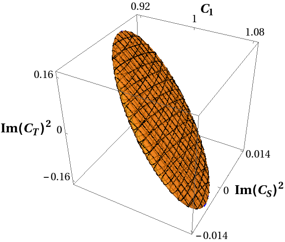
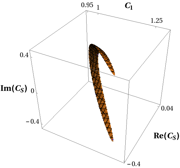
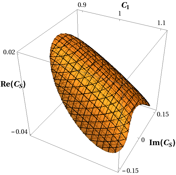
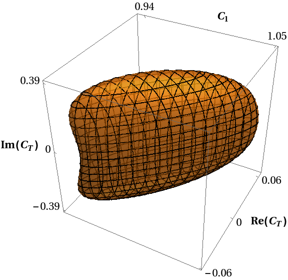
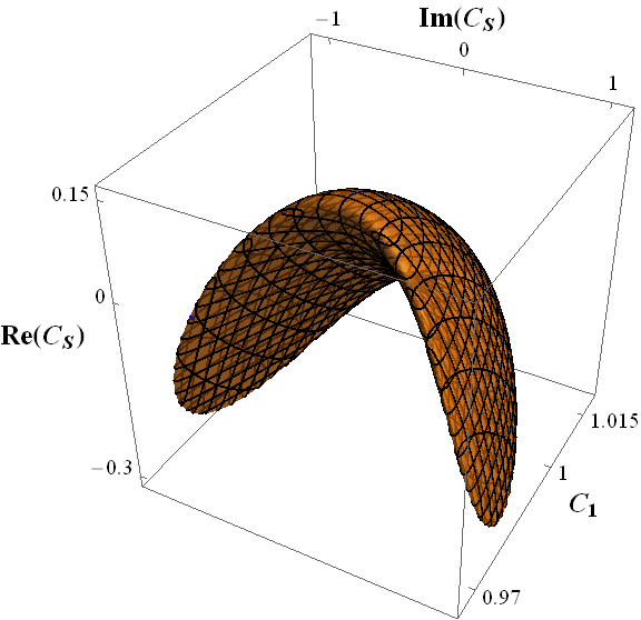
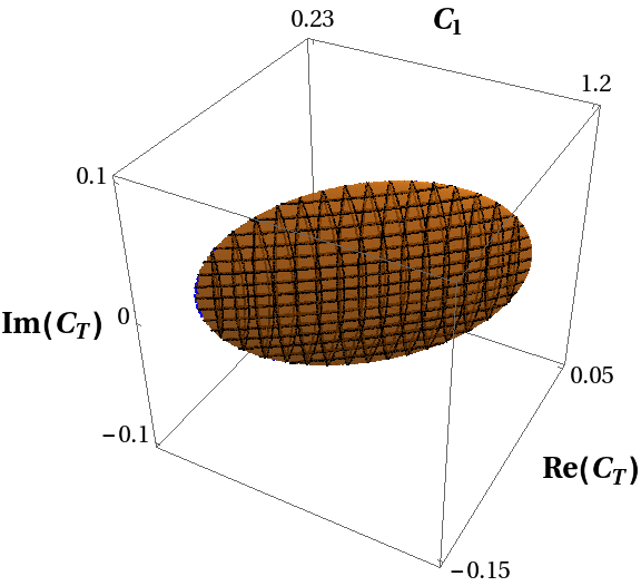
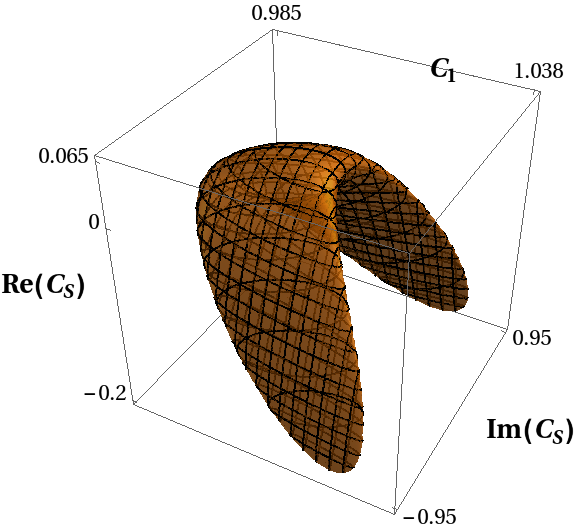
Figure 1: Surfaces of constant χ2=1superscript𝜒21\chi^{2}=1 for a few selected cases of different observables in BDτντ𝐵𝐷𝜏subscript𝜈𝜏B\to D\tau\nu_{\tau}.
Refer to caption
(a) Case fsuperscript𝑓{\it f^{*}} (R(D)𝑅superscript𝐷R(D^{*}))
Refer to caption
(b) Case gsuperscript𝑔{\it g^{*}} (R(D)𝑅superscript𝐷R(D^{*}))
Refer to caption
(c) Case hsuperscript{\it h^{*}} (R(D)𝑅superscript𝐷R(D^{*}))
Refer to caption
(d) Case isuperscript𝑖{\it i^{*}} (R(D)𝑅superscript𝐷R(D^{*}))
Refer to caption
(e) Case fsuperscript𝑓{\it f^{*}} (PτRsuperscriptsubscript𝑃𝜏superscript𝑅P_{\tau}^{R^{*}})
Refer to caption
(f) Case gsuperscript𝑔{\it g^{*}} (PτRsuperscriptsubscript𝑃𝜏superscript𝑅P_{\tau}^{R^{*}})
Refer to caption
(g) Case hsuperscript{\it h^{*}} (PτRsuperscriptsubscript𝑃𝜏superscript𝑅P_{\tau}^{R^{*}})
Refer to caption
(h) Case isuperscript𝑖{\it i^{*}} (PτRsuperscriptsubscript𝑃𝜏superscript𝑅P_{\tau}^{R^{*}})
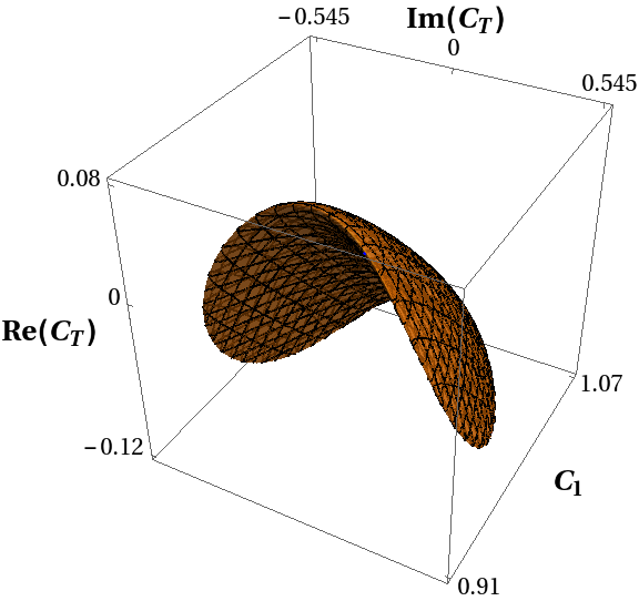
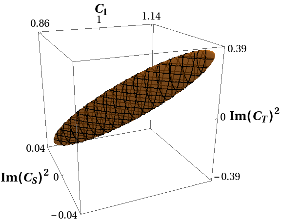
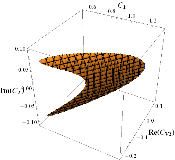
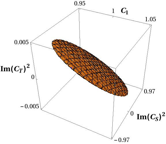
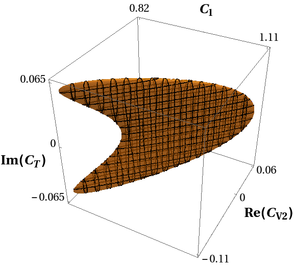
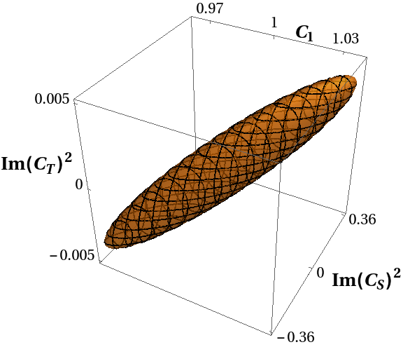
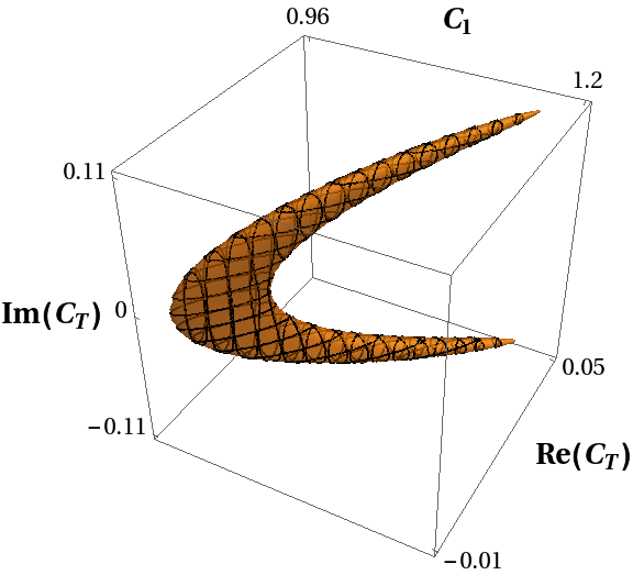
Figure 2: Surfaces of constant χ2=1superscript𝜒21\chi^{2}=1 for a few selected cases of different observables shown in BDτντ𝐵superscript𝐷𝜏subscript𝜈𝜏B\to D^{\ast}\tau\nu_{\tau}.

In some more simplified cases, where the number of non-zero NP parameters are less, we compute the χ2superscript𝜒2\chi^{2}, which is defined as

χ2superscript𝜒2\displaystyle\chi^{2} =i,j(CiCi0)(CjCj0)Vij1,absentsubscript𝑖𝑗subscript𝐶𝑖superscriptsubscript𝐶𝑖0subscript𝐶𝑗superscriptsubscript𝐶𝑗0superscriptsubscript𝑉𝑖𝑗1\displaystyle=\sum_{i,j}(C_{i}-C_{i}^{0})(C_{j}-C_{j}^{0})V_{ij}^{-1},~{}
where, Vijwhere, subscript𝑉𝑖𝑗\displaystyle\text{where, }~{}~{}~{}V_{ij} =XijσPeff.absentsubscript𝑋𝑖𝑗subscriptsubscript𝜎𝑃subscript𝑒𝑓𝑓\displaystyle=\frac{X_{ij}}{{\cal B}_{\ell}~{}\sigma_{P}~{}{\cal L}_{eff}}. (13)

The Ci0superscriptsubscript𝐶𝑖0C_{i}^{0}s are the seed values, which can be considered as model inputs; as discussed earlier, we choose Ci0=0superscriptsubscript𝐶𝑖00C_{i}^{0}=0, for i1𝑖1i\neq 1, and C10=1superscriptsubscript𝐶101C_{1}^{0}=1. The χ2=1superscript𝜒21\chi^{2}=1 surfaces are perfect ellipsoids in Cisubscript𝐶𝑖C_{i} basis, and they indicate the ±1σplus-or-minus1𝜎\pm 1\sigma errors in the determination of Cisubscript𝐶𝑖C_{i}s. The constant χ2=1superscript𝜒21\chi^{2}=1 surfaces are shown in Figs. 1, and 2. The largest and the smallest values in the figures represent ±1σplus-or-minus1𝜎\pm 1\sigma errors of corresponding parameters.

|δCi|𝛿subscript𝐶𝑖|\delta C_{i}| Cases b c d e f
|δC1|𝛿subscript𝐶1|\delta C_{1}| 0.27 0.27 0.04 0.07 0.07
|δRe(CS)|𝛿𝑅𝑒subscript𝐶𝑆|\delta Re(C_{S})| 0.40 - - 0.05 -
|δRe(CT)|𝛿𝑅𝑒subscript𝐶𝑇|\delta Re(C_{T})| - 0.30 - - 0.04
|δ(Im(CS)Im(CT))|𝛿𝐼𝑚subscript𝐶𝑆𝐼𝑚subscript𝐶𝑇|\delta(Im(C_{S})Im({C_{T}}))| 0.11 0.11 0.01 - -
Table 9: Numerical values of |δCi|𝛿subscript𝐶𝑖|\delta C_{i}| extracted from the τ𝜏\tau forward-backward asymmetry in BDτντ𝐵𝐷𝜏subscript𝜈𝜏B\to D\tau\nu_{\tau}.

III.1 Discussions

For case a, the uncertainties obtained from the simultaneous extraction of all the Wilson coefficients from the observable R(D)𝑅𝐷R(D) shows that 444The results corresponding to the case a are not shown in the table, because the extracted uncertainties are very large (>>1)much-greater-thanabsent1(>>1).

|δC4||δC5||δRe(CS)||δRe(CT)|1,δ|CS|2δ|CT|22,formulae-sequence𝛿subscript𝐶4𝛿subscript𝐶5𝛿𝑅𝑒subscript𝐶𝑆𝛿𝑅𝑒subscript𝐶𝑇similar-to1similar-to𝛿superscriptsubscript𝐶𝑆2𝛿superscriptsubscript𝐶𝑇22\frac{|\delta C_{4}|}{|\delta C_{5}|}\approx\frac{|\delta Re(C_{S})|}{|\delta Re(C_{T})|}\sim 1,\,\,\,\,\,\,\frac{\delta|C_{S}|^{2}}{\delta|C_{T}|^{2}}\sim 2, (14)

which shows that R(D)𝑅𝐷R(D) is equally sensitive to the real part of CSsubscript𝐶𝑆C_{S} and CTsubscript𝐶𝑇C_{T}. The above result does not allow a direct comparison between the sensitivities to the imaginary part of the coefficients. The results obtained for all the other cases are shown in Tab. 7, and in Figs.1a, 1b and 1c. We note that if the Wilson coefficients are purely imaginary then R(D)𝑅𝐷R(D) is more sensitive to Im(CS)𝐼𝑚subscript𝐶𝑆Im(C_{S}) compared to Im(CT)𝐼𝑚subscript𝐶𝑇Im(C_{T}). Also, it is important to note that this observable is more sensitive to the real part of the coefficients than the imaginary part. Comparing all the different cases considered for R(D)𝑅𝐷R(D), it would be difficult to comment on the overall sensitivity of this observable to a particular type of NP interaction. However, in the next section we will see that there are distinct regions of q2superscript𝑞2q^{2} which are sensitive to either scalar or tensor type interactions.

On the other hand, the analysis of PτR(q2)superscriptsubscript𝑃𝜏𝑅superscript𝑞2P_{\tau}^{R}(q^{2}) for case a gives

|δC4||δC5||δRe(CS)||δRe(CT)|0.5,δ|CS|2δ|CT|22,formulae-sequence𝛿subscript𝐶4𝛿subscript𝐶5𝛿𝑅𝑒subscript𝐶𝑆𝛿𝑅𝑒subscript𝐶𝑇similar-to0.5similar-to𝛿superscriptsubscript𝐶𝑆2𝛿superscriptsubscript𝐶𝑇22\frac{|\delta C_{4}|}{|\delta C_{5}|}\approx\frac{|\delta Re(C_{S})|}{|\delta Re(C_{T})|}\sim 0.5,\,\,\,\,\,\,\frac{\delta|C_{S}|^{2}}{\delta|C_{T}|^{2}}\sim 2, (15)

which shows an improvement in sensitivity to Re(CS)𝑅𝑒subscript𝐶𝑆Re(C_{S}) compared to Re(CT)𝑅𝑒subscript𝐶𝑇Re(C_{T}). The results obtained from all the other relevant cases are shown in Table 7, and in Figs. 1d, 1e, and 1f, which allow a case by case comparison between the results obtained from R(D)𝑅𝐷R(D) and PτRsuperscriptsubscript𝑃𝜏𝑅P_{\tau}^{R}. Interestingly, the extracted uncertainties are less compared to that extracted in R(D)𝑅𝐷R(D). The sensitivity of this observable to tensor interaction is a little less, compared to scalar interaction, but it can be extracted with uncertainties less than 1.

As shown in Table 8, and in Fig. 2, the observables like R(D)𝑅superscript𝐷R(D^{*}) and PτRsuperscriptsubscript𝑃𝜏superscript𝑅P_{\tau}^{R^{*}} are more sensitive to |CT|2superscriptsubscript𝐶𝑇2|C_{T}|^{2} compared to any other new Wilson coefficients, almost in all the cases |CT|2superscriptsubscript𝐶𝑇2|C_{T}|^{2} and Re(CT)𝑅𝑒subscript𝐶𝑇Re(C_{T}) can be extracted with small uncertainties. A case by case comparison shows that the above observables are more sensitive to CTsubscript𝐶𝑇C_{T} than CSsubscript𝐶𝑆C_{S}, and δRe(CT)<δRe(CV2)𝛿𝑅𝑒subscript𝐶𝑇𝛿𝑅𝑒subscript𝐶subscript𝑉2\delta Re(C_{T})<\delta Re(C_{V_{2}}) but they are of same order. Also, when CTsubscript𝐶𝑇C_{T} is purely imaginary, we find δIm(CT)δRe(CV2)𝛿𝐼𝑚subscript𝐶𝑇𝛿𝑅𝑒subscript𝐶subscript𝑉2\delta Im(C_{T})\approx\delta Re(C_{V_{2}}), though PτRsuperscriptsubscript𝑃𝜏superscript𝑅P_{\tau}^{R^{*}} have little better sensitivity to Im(CT)𝐼𝑚subscript𝐶𝑇Im(C_{T}). Therefore, these observables alone won’t allow us to distinguish the contributions from right handed vector current to that of a tensor current. However, in the next section we will see that a bin by bin analysis of the q2superscript𝑞2q^{2} distribution of the differential decay rate allows to discriminate the effects of these interactions.

However, when CT=0subscript𝐶𝑇0C_{T}=0, both the observables are almost equally sensitive, though δRe(CS)<δRe(CV2)𝛿𝑅𝑒subscript𝐶𝑆𝛿𝑅𝑒subscript𝐶subscript𝑉2\delta Re(C_{S})<\delta Re(C_{V_{2}}), to the real part of the vector and scalar Wilson coefficients. In case CSsubscript𝐶𝑆C_{S} is purely imaginary, δRe(CV2)<<δIm(CS)much-less-than𝛿𝑅𝑒subscript𝐶subscript𝑉2𝛿𝐼𝑚subscript𝐶𝑆\delta Re(C_{V_{2}})<<\delta Im(C_{S}) i.e the observables are less sensitive to the imaginary part of CSsubscript𝐶𝑆C_{S} compared to the real parts of CV2subscript𝐶subscript𝑉2C_{V_{2}} and CSsubscript𝐶𝑆C_{S}. Again, we note that the extracted errors on Cisubscript𝐶𝑖C_{i}s from PτRsuperscriptsubscript𝑃𝜏superscript𝑅P_{\tau}^{R^{*}} are smaller than those in R(D)𝑅superscript𝐷R(D^{*}).

|δCi|𝛿subscript𝐶𝑖|\delta C_{i}| Cases 2superscript22^{*} 3superscript33^{*} 4superscript44^{*} 5superscript55^{*} 6superscript66^{*} 7superscript77^{*}
|δC1|𝛿subscript𝐶1|\delta C_{1}| 1.30 2.41 0.40 0.27 0.52 0.04
δ|CT|2𝛿superscriptsubscript𝐶𝑇2\delta|C_{T}|^{2} 0.12 0.08 0.04 0.04 0.03 -
|δRe(CS)|𝛿𝑅𝑒subscript𝐶𝑆|\delta Re(C_{S})| 16.30 - 1.72 - - 0.02
|δRe(CT)|𝛿𝑅𝑒subscript𝐶𝑇|\delta Re(C_{T})| - 1.06 - 0.12 - -
|δ(Im(CS)Im(CT))|𝛿𝐼𝑚subscript𝐶𝑆𝐼𝑚superscriptsubscript𝐶𝑇|\delta(Im(C_{S})Im({C_{T}}^{*}))| 2.48 2.41 - - 0.26 -
Table 10: Numerical values of |δCi|𝛿subscript𝐶𝑖|\delta C_{i}| extracted from τ𝜏\tau forward backward asymmetry in BDτντ𝐵superscript𝐷𝜏subscript𝜈𝜏B\to D^{\ast}\tau\nu_{\tau}.

The results of the analysis of forward-backward asymmetries and Dsuperscript𝐷D^{*} polarisation are given in Tables 9, 10, and 11 respectively. The forward-backward asymmetry in BDτντ𝐵𝐷𝜏subscript𝜈𝜏B\to D\tau\nu_{\tau} is equally sensitive to the scalar and tensor type interactions.

For case 1superscript11^{*} in AFBRsuperscriptsubscript𝐴𝐹𝐵superscript𝑅A_{FB}^{R^{*}}, we find

δC1δ|CT|21,δC2δ|CT|224,formulae-sequence𝛿subscript𝐶1𝛿superscriptsubscript𝐶𝑇21𝛿subscript𝐶2𝛿superscriptsubscript𝐶𝑇224\frac{\delta C_{1}}{\delta|C_{T}|^{2}}\approx 1,\ \ \ \ \frac{\delta C_{2}}{\delta|C_{T}|^{2}}\approx 24, (16)

and

δC2δRe(CT)12,𝛿subscript𝐶2𝛿𝑅𝑒subscript𝐶𝑇12\frac{\delta C_{2}}{\delta Re(C_{T})}\approx 12, (17)

where C1subscript𝐶1C_{1} and C2subscript𝐶2C_{2} are the functions of the Wilson coefficients of the vector operators. The approximate forms are given by

C11+2Re(CV1),C21+2Re(CV1)2Re(CV2).formulae-sequencesubscript𝐶112𝑅𝑒subscript𝐶subscript𝑉1subscript𝐶212𝑅𝑒subscript𝐶subscript𝑉12𝑅𝑒subscript𝐶subscript𝑉2C_{1}\approx 1+2Re(C_{V_{1}}),\ C_{2}\approx 1+2Re(C_{V_{1}})-2Re(C_{V_{2}}). (18)

It indicates that the τ𝜏\tau forward-backward asymmetry in BDτντ𝐵superscript𝐷𝜏subscript𝜈𝜏B\to D^{\ast}\tau\nu_{\tau} is more sensitive to tensor Wilson coefficients than to a vector, in particular to CV2subscript𝐶subscript𝑉2C_{V_{2}}. In order to understand it better, we define

C12=C1C22Re(CV2).subscript𝐶12subscript𝐶1subscript𝐶22𝑅𝑒subscript𝐶subscript𝑉2C_{12}=C_{1}-C_{2}\approx 2Re(C_{V_{2}}). (19)

Therefore, a simple calculation shows that

δRe(CV2)δRe(CT)=12δC12δRe(CT)6.𝛿𝑅𝑒subscript𝐶subscript𝑉2𝛿𝑅𝑒subscript𝐶𝑇12𝛿subscript𝐶12𝛿𝑅𝑒subscript𝐶𝑇6\frac{\delta Re(C_{V_{2}})}{\delta Re(C_{T})}=\frac{1}{2}\frac{\delta C_{12}}{\delta Re(C_{T})}\approx 6. (20)

In all the other cases with CV2=0subscript𝐶subscript𝑉20C_{V_{2}}=0, the AFBsubscript𝐴𝐹𝐵A_{FB} in BDτντ𝐵superscript𝐷𝜏subscript𝜈𝜏B\to D^{\ast}\tau\nu_{\tau} is more sensitive to the tensor interaction compared to the scalar. On the other hand the Dsuperscript𝐷D^{*} polarisation is equally sensitive to the scalar and tensor interactions. Therefore, if future data shows large deviations from the SM predictions in all the observables like R(D)𝑅superscript𝐷R(D^{*}), AFBsuperscriptsubscript𝐴𝐹𝐵A_{FB}^{*}, and Dsuperscript𝐷D^{*} polarisation, that can be thought of as an indication of the presence of a new tensor type interaction. On other hand, if a deviation is only in R(D)𝑅superscript𝐷R(D^{*}) and not in the others, that could be an indication of a new vector interaction.

|δCi|𝛿subscript𝐶𝑖|\delta C_{i}| Cases A𝐴A B𝐵B C𝐶C D𝐷D E𝐸E F𝐹F G𝐺G H𝐻H
|δC1|𝛿subscript𝐶1|\delta C_{1}| 3.58 0.74 1.41 0.12 0.05 1.41 0.05 0.1
δ|CS|2𝛿superscriptsubscript𝐶𝑆2\delta|C_{S}|^{2} 16.63 3.39 0.55 0.55 0.77 - 0.54 -
δ|CT|2𝛿superscriptsubscript𝐶𝑇2\delta|C_{T}|^{2} 2.53 0.09 0.41 0.01 - 0.41 - 0.01
|δRe(CS)|𝛿𝑅𝑒subscript𝐶𝑆|\delta Re(C_{S})| 7.05 1.40 - - 0.20 - - -
|δRe(CT)|𝛿𝑅𝑒subscript𝐶𝑇|\delta Re(C_{T})| 5.07 - 1.00 - - 1.00 - -
Table 11: The results obtained from the analysis of the Dsuperscript𝐷D^{\ast} polarisation asymmetry in the decay BDτντ𝐵superscript𝐷𝜏subscript𝜈𝜏B\to D^{\ast}\tau\nu_{\tau}.

III.2 Bin-by-bin analysis

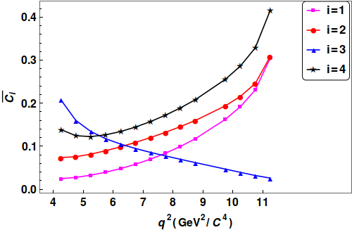
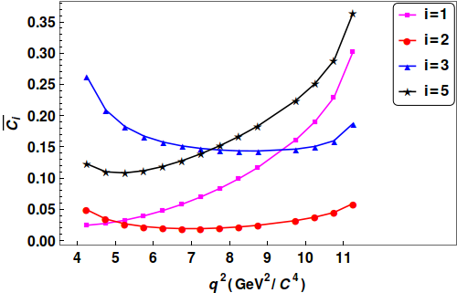
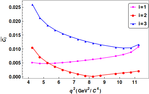
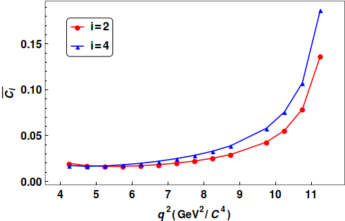
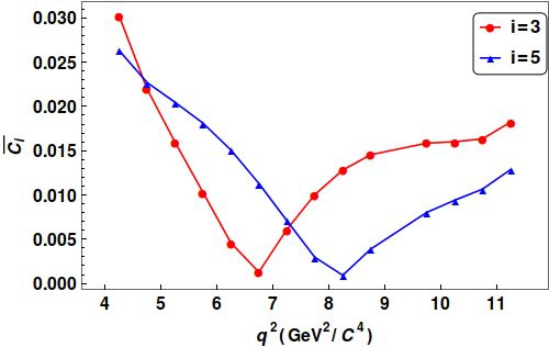
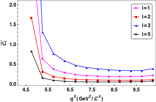
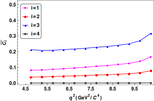
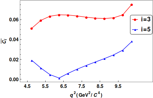
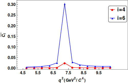
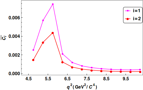
In general, the sensitivity to various NP interactions may also be q2superscript𝑞2q^{2} dependent. Hence, we analyse the bin-by-bin q2superscript𝑞2q^{2} distribution of the differential decay rate of BD()τντ𝐵superscript𝐷𝜏subscript𝜈𝜏B\to D^{(\ast)}\tau\nu_{\tau} to look for more possibilities, and zoom in to the regions of q2superscript𝑞2q^{2}, within which the sensitivity to a specific type of new interaction is much larger than most other regions. In general the δCi𝛿subscript𝐶𝑖\delta C_{i}s extracted from individual bins are very large, therefore in the figs. 3, 4 we plot δCi¯=δCi/Nnorm¯𝛿subscript𝐶𝑖𝛿subscript𝐶𝑖subscript𝑁𝑛𝑜𝑟𝑚\bar{\delta C_{i}}=\delta C_{i}/N_{norm}, where Nnormsubscript𝑁𝑛𝑜𝑟𝑚N_{norm} is some number used to normalised δCi𝛿subscript𝐶𝑖\delta C_{i}.

Refer to caption
(a) Case b𝑏b with C2=|CS|2subscript𝐶2superscriptsubscript𝐶𝑆2C_{2}=|C_{S}|^{2}, C3=Im(CT)2subscript𝐶3𝐼𝑚superscriptsubscript𝐶𝑇2C_{3}=Im(C_{T})^{2}, C4=Re(CS)subscript𝐶4𝑅𝑒subscript𝐶𝑆C_{4}=Re(C_{S}), and Nnorm=105subscript𝑁𝑛𝑜𝑟𝑚superscript105N_{norm}=10^{5}.
Refer to caption
(b) Case c𝑐c with C2=Im(CS)2subscript𝐶2𝐼𝑚superscriptsubscript𝐶𝑆2C_{2}=Im(C_{S})^{2}, C3=|CT|2subscript𝐶3superscriptsubscript𝐶𝑇2C_{3}=|C_{T}|^{2}, C5=Re(CT)subscript𝐶5𝑅𝑒subscript𝐶𝑇C_{5}=Re(C_{T}), and Nnorm=105subscript𝑁𝑛𝑜𝑟𝑚superscript105N_{norm}=10^{5}.
Refer to caption
(c) Case d𝑑d with C2=Im(CS)2subscript𝐶2𝐼𝑚superscriptsubscript𝐶𝑆2C_{2}=Im(C_{S})^{2}, C3=Im(CT)2subscript𝐶3𝐼𝑚superscriptsubscript𝐶𝑇2C_{3}=Im(C_{T})^{2}, and Nnorm=104subscript𝑁𝑛𝑜𝑟𝑚superscript104N_{norm}=10^{4}.
Refer to caption
(d) Case e𝑒e with C2=|CS|2subscript𝐶2superscriptsubscript𝐶𝑆2C_{2}=|C_{S}|^{2}, C4=Re(CS)subscript𝐶4𝑅𝑒subscript𝐶𝑆C_{4}=Re(C_{S}), and Nnorm=104subscript𝑁𝑛𝑜𝑟𝑚superscript104N_{norm}=10^{4}.
Refer to caption
(e) Case f𝑓f with C3=|CT|2subscript𝐶3superscriptsubscript𝐶𝑇2C_{3}=|C_{T}|^{2}, C5=Re(CT)subscript𝐶5𝑅𝑒subscript𝐶𝑇C_{5}=Re(C_{T}), and Nnorm=104subscript𝑁𝑛𝑜𝑟𝑚superscript104N_{norm}=10^{4}
Figure 3: Selected cases in BDτντ𝐵𝐷𝜏subscript𝜈𝜏B\to D\tau\nu_{\tau}, here, Ci¯=|δCi|/Nnorm¯subscript𝐶𝑖𝛿subscript𝐶𝑖subscript𝑁𝑛𝑜𝑟𝑚\overline{C_{i}}=|\delta C_{i}|/N_{norm}.

The results obtained from the analysis of the q2superscript𝑞2q^{2} distribution of differential decay rate in BDτντ𝐵𝐷𝜏subscript𝜈𝜏B\to D\tau\nu_{\tau} are presented in fig. 3, where the variations of the δCi𝛿subscript𝐶𝑖\delta C_{i}s with q2superscript𝑞2q^{2} are shown. The normalised uncertainties in the simultaneous extraction of |CS|2superscriptsubscript𝐶𝑆2|C_{S}|^{2}, |CT|2superscriptsubscript𝐶𝑇2|C_{T}|^{2}, Re(CT)𝑅𝑒subscript𝐶𝑇Re(C_{T}) and Re(CS)𝑅𝑒subscript𝐶𝑆Re(C_{S}), and their variations with q2superscript𝑞2q^{2} are shown in figs. 3a and 3b respectively. On the other hand the variations of δ|CS|2𝛿superscriptsubscript𝐶𝑆2\delta|C_{S}|^{2}, and δRe(CS)𝛿𝑅𝑒subscript𝐶𝑆\delta Re(C_{S}) with q2superscript𝑞2q^{2} when CT=0subscript𝐶𝑇0C_{T}=0 are shown in fig. 3d, while that for δ|CT|2𝛿superscriptsubscript𝐶𝑇2\delta|C_{T}|^{2}, and δRe(CT)𝛿𝑅𝑒subscript𝐶𝑇\delta Re(C_{T}) when CS=0subscript𝐶𝑆0C_{S}=0 are shown in fig. 3e. We note that in the low q2superscript𝑞2q^{2} region (<7𝐺𝑒𝑉2/c4<absent7superscript𝐺𝑒𝑉2superscript𝑐4\mathrel{\raise 1.29167pt\hbox{$<$\kern-7.5pt\lower 4.30554pt\hbox{$\sim$}}}7{\it GeV}^{2}/c^{4}) the differential decay rate is sensitive to the scalar interaction 555In very low q2superscript𝑞2q^{2} regions the q2superscript𝑞2q^{2} distribution is also sensitive to C1subscript𝐶1C_{1}., the sensitivity to tensor interaction in this region is very weak, whereas in the high q2superscript𝑞2q^{2} region (>7𝐺𝑒𝑉2/c4>absent7superscript𝐺𝑒𝑉2superscript𝑐4\mathrel{\raise 1.29167pt\hbox{$>$\kern-7.5pt\lower 4.30554pt\hbox{$\sim$}}}7{\it GeV}^{2}/c^{4}) it is rather sensitive to the tensor interaction. In case the Wilson coefficients are purely imaginary, in all the q2superscript𝑞2q^{2} regions, the decay rate distribution is sensitive more to the scalar interaction (fig. 3c) than the others.

As we noted earlier, R(D)𝑅superscript𝐷R(D^{*}) is equally sensitive to CV2subscript𝐶subscript𝑉2C_{V_{2}} and CTsubscript𝐶𝑇C_{T} (case asuperscript𝑎a^{*}), however, the analysis of the differential decay rate distributions show that (figs. 4e and 4d) it is sensitive to tensor interaction only in the very high and low q2superscript𝑞2q^{2} regions, and it is sensitive to CV2subscript𝐶subscript𝑉2C_{V_{2}} in all the q2superscript𝑞2q^{2} regions except the very low q2superscript𝑞2q^{2} region. In fig. 4a the variations of δRe(CV2)𝛿𝑅𝑒subscript𝐶subscript𝑉2\delta Re(C_{V_{2}}), δRe(CS)𝛿𝑅𝑒subscript𝐶𝑆\delta Re(C_{S}), and δ|CS|2𝛿superscriptsubscript𝐶𝑆2\delta|C_{S}|^{2} with the q2superscript𝑞2q^{2} in the case CT=0subscript𝐶𝑇0C_{T}=0 are shown, we note that in all the q2superscript𝑞2q^{2} regions the decay rate is equally sensitive to vector and scalar interactions except in the very low q2superscript𝑞2q^{2} region, where the sensitivity to Re(CS)𝑅𝑒subscript𝐶𝑆Re(C_{S}) is better than that to Re(CV2)𝑅𝑒subscript𝐶subscript𝑉2Re(C_{V_{2}}). We also study the cases when the NP interaction is scalar type. The q2superscript𝑞2q^{2} distribution of the extracted errors on the respective parameters is shown in fig. 4c, which indicates that the decay rate is sensitive to scalar interactions only in the low q2superscript𝑞2q^{2} region. If CSsubscript𝐶𝑆C_{S} and CTsubscript𝐶𝑇C_{T} are purely imaginary than the q2superscript𝑞2q^{2} distribution of the decay rate is sensitive to the tensor interactions in all the q2superscript𝑞2q^{2} regions (fig. 4b).

Refer to caption
(a) Case csuperscript𝑐c^{*} with C2=Re(CV2)subscript𝐶2𝑅𝑒subscript𝐶subscript𝑉2C_{2}=Re(C_{V_{2}}), C3=|CS|2subscript𝐶3superscriptsubscript𝐶𝑆2C_{3}=|C_{S}|^{2}, C5=Re(CS)subscript𝐶5𝑅𝑒subscript𝐶𝑆C_{5}=Re(C_{S}), and Nnorm=106subscript𝑁𝑛𝑜𝑟𝑚superscript106N_{norm}=10^{6}.
Refer to caption
(b) Case jsuperscript𝑗j^{*} with C2=Re(CV2)subscript𝐶2𝑅𝑒subscript𝐶subscript𝑉2C_{2}=Re(C_{V_{2}}), C3=Im(CT)2subscript𝐶3𝐼𝑚superscriptsubscript𝐶𝑇2C_{3}=Im(C_{T})^{2}, C4=Im(CS)2subscript𝐶4𝐼𝑚superscriptsubscript𝐶𝑆2C_{4}=Im(C_{S})^{2}, and Nnorm=106subscript𝑁𝑛𝑜𝑟𝑚superscript106N_{norm}=10^{6}.
Refer to caption
(c) Case hsuperscripth^{*} with C3=|CS|2subscript𝐶3superscriptsubscript𝐶𝑆2C_{3}=|C_{S}|^{2}, C5=Re(CS)subscript𝐶5𝑅𝑒subscript𝐶𝑆C_{5}=Re(C_{S}), and Nnorm=104subscript𝑁𝑛𝑜𝑟𝑚superscript104N_{norm}=10^{4}
Refer to caption
(d) Case isuperscript𝑖i^{*} with C4=|CT|2subscript𝐶4superscriptsubscript𝐶𝑇2C_{4}=|C_{T}|^{2}, C6=Re(CT)subscript𝐶6𝑅𝑒subscript𝐶𝑇C_{6}=Re(C_{T}), and Nnorm=104subscript𝑁𝑛𝑜𝑟𝑚superscript104N_{norm}=10^{4}
Refer to caption
(e) Case ksuperscript𝑘k^{*} with C2=Re(CV2)subscript𝐶2𝑅𝑒subscript𝐶subscript𝑉2C_{2}=Re(C_{V_{2}}) and Nnorm=104subscript𝑁𝑛𝑜𝑟𝑚superscript104N_{norm}=10^{4}
Figure 4: Selected cases in BDτντ𝐵superscript𝐷𝜏subscript𝜈𝜏B\to D^{\ast}\tau\nu_{\tau}, here, Ci¯=|δCi|/Nnorm¯subscript𝐶𝑖𝛿subscript𝐶𝑖subscript𝑁𝑛𝑜𝑟𝑚\overline{C_{i}}=|\delta C_{i}|/N_{norm}.

All these studies suggest that we could gain in NP sensitivity if we focus on specific q2superscript𝑞2q^{2} regions, which we may lose in the full q2superscript𝑞2q^{2}-integrated observables. We note that the sensitivity to a particular type of interaction is limited to particular regions of q2superscript𝑞2q^{2}. Therefore, the experimental data in the specific regions of q2superscript𝑞2q^{2} could help us a better interpretation of the type of NP interactions, which may not be obtainable from q2superscript𝑞2q^{2} integrated observables. As for example, if we see large deviations in data only in the very high and very low q2superscript𝑞2q^{2} regions, that can be interpreted as due to the presence of a tensor interaction (fig. 4d). On the other hand, if we see deviations only in the low q2superscript𝑞2q^{2} (<7absent7<7) bins, that could be due to a new scalar interaction (fig. 4c). Finally, if data shows deviations in most of the q2superscript𝑞2q^{2} bin except the very low q2superscript𝑞2q^{2}, this can be due to the presence of new vector interaction (fig. 4e).
Refer to caption
(a)
Refer to caption
(b)
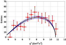
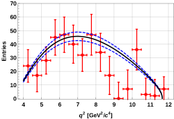
Figure 5: Measured q2superscript𝑞2q^{2} distribution of the events in BDτντ𝐵𝐷𝜏subscript𝜈𝜏B\to D\tau\nu_{\tau} (left) and BDτντ𝐵superscript𝐷𝜏subscript𝜈𝜏B\to D^{\ast}\tau\nu_{\tau} (right) decays Lees:2013uzd . The black lines represent the q2superscript𝑞2q^{2} distribution predicted in the SM, obtained from the respective differential branching fractions.

In order to explain our point we take the example of the q2superscript𝑞2q^{2} distributions of the measured events in BD()τντ𝐵superscript𝐷𝜏subscript𝜈𝜏B\to D^{(\ast)}\tau\nu_{\tau}, which are shown in Fig.(5). The plots are generated using the data given in ref. Lees:2013uzd ; Aubert:2009 ; Aubert:2007 . The predicted q2superscript𝑞2q^{2} distributions in SM with the central values of the form factors are shown by black lines, blue dotted lines represent the errors in SM. In Fig.(5a), we see that the data is not fully consistent with the SM in the region 8.0<q2<118.0superscript𝑞2118.0<q^{2}<11, which is the region where the decay rate distribution is sensitive to tensor interaction, as analysed above in the decay BDτντ𝐵𝐷𝜏subscript𝜈𝜏B\to D\tau\nu_{\tau}. At the moment it is hard to conclude anything, and we have to wait for better statistics. From Fig.(5b) we see distinct regions of q2superscript𝑞2q^{2} where the data is not fully consistent with the SM prediction, and our analysis suggests that those regions could potentially be very sensitive to NP effects. Again, because of poor statistics it is premature to conclude anything. Therefore, the experimental effort should be in gathering more statistics in specific regions of q2superscript𝑞2q^{2} potentially sensitive to NP, which may in turn help the clean extraction of NP couplings.

As mentioned above, the numerical estimates are done with central values of all the relevant parameters taken from formfactors . Numerical instability of our results could be main source of uncertainty in our estimates. The numerical results of Xijsubscript𝑋𝑖𝑗X_{ij}, which depend on the matrix inversion of Mijsubscript𝑀𝑖𝑗M_{ij}, are often unstable; even a tiny variation of Mijsubscript𝑀𝑖𝑗M_{ij} could change Xijsubscript𝑋𝑖𝑗X_{ij} significantly. This is why, when we estimate the statistical uncertainties in simultaneous extractions of the Wilson coefficients, we allowed only stable solutions. We calculate the selected δCi𝛿subscript𝐶𝑖\delta C_{i} first to mthsuperscript𝑚𝑡m^{th} and then to (m1)thsuperscript𝑚1𝑡(m-1)^{th} decimal places, and obtain δCi[m]𝛿superscriptsubscript𝐶𝑖delimited-[]𝑚{\delta C_{i}}^{[m]} and δCi[(m1)]𝛿superscriptsubscript𝐶𝑖delimited-[]𝑚1{\delta C_{i}}^{[(m-1)]} respectively. We consider the results as stable only when (δCi[m]δCi[(m1)])/δCi[m]<0.01𝛿superscriptsubscript𝐶𝑖delimited-[]𝑚𝛿superscriptsubscript𝐶𝑖delimited-[]𝑚1𝛿superscriptsubscript𝐶𝑖delimited-[]𝑚0.01({\delta C_{i}}^{[m]}-{\delta C_{i}}^{[(m-1)]})/{\delta C_{i}}^{[m]}<0.01. We checked the stability up to m=10𝑚10m=10, and in most of the cases presented above, our results are very much stable, and the error due to this is negligible. As we can see from the expressions of δCi𝛿subscript𝐶𝑖\delta C_{i}, the other sources of errors in our estimates are given by the errors in fi(q2)subscript𝑓𝑖superscript𝑞2f_{i}(q^{2}), σPsubscript𝜎𝑃\sigma_{P} , effsubscript𝑒𝑓𝑓{\cal L}_{eff} , and subscript{\cal B}_{\ell}. It is straight forward to estimate the errors due to σPsubscript𝜎𝑃\sigma_{P} , effsubscript𝑒𝑓𝑓{\cal L}_{eff} , and subscript{\cal B}_{\ell}.

Cases δCi𝛿subscript𝐶𝑖\delta C_{i} δCi+𝛿superscriptsubscript𝐶𝑖{\delta C_{i}}^{+} δCi𝛿superscriptsubscript𝐶𝑖{\delta C_{i}}^{-} ±%Err.\pm\%Err.
d C1subscript𝐶1C_{1} 0.082 0.079 0.087 5.032
Im(CS)2𝐼𝑚superscriptsubscript𝐶𝑆2Im(C_{S})^{2} 0.013 0.013 0.014 5.032
Im(CT)2𝐼𝑚superscriptsubscript𝐶𝑇2Im(C_{T})^{2} 0.168 0.160 0.177 5.032
e C1subscript𝐶1C_{1} 0.240 0.229 0.253 5.031
|CS|2superscriptsubscript𝐶𝑆2|C_{S}|^{2} 0.274 0.261 0.289 5.031
Re(CS)𝑅𝑒subscript𝐶𝑆Re(C_{S}) 0.354 0.337 0.373 5.031
Table 12: Numerical values of δCi𝛿subscript𝐶𝑖\delta C_{i}s, and δCi+𝛿superscriptsubscript𝐶𝑖{\delta C_{i}}^{+} (δCi𝛿superscriptsubscript𝐶𝑖{\delta C_{i}}^{-}) considering +10% (-10%) errors in fi(q2)subscript𝑓𝑖superscript𝑞2f_{i}(q^{2}) for few cases of R(D)𝑅𝐷R(D). The % error is given by (δCiδCi±)/δCi𝛿subscript𝐶𝑖𝛿superscriptsubscript𝐶𝑖plus-or-minus𝛿subscript𝐶𝑖(\delta C_{i}-{\delta C_{i}}^{\pm})/{\delta C_{i}}.

However, the estimate due to fi(q2)subscript𝑓𝑖superscript𝑞2f_{i}(q^{2})s are not that straight forward since Mijsubscript𝑀𝑖𝑗M_{ij}s depend solely upon them. The main sources of uncertainties in fisubscript𝑓𝑖f_{i}s, including the SM, are the form-factors. Errors due to other parameters, like CKM element etc, are canceled in the ratios. In the tables 12, and 13, we consider a few cases and give a rough estimate of the uncertainties due to the errors in fi(q2)subscript𝑓𝑖superscript𝑞2f_{i}(q^{2}). The overall error is about ±plus-or-minus\pm 5% in the extraction of δCi𝛿subscript𝐶𝑖\delta C_{i}s, if we consider the errors in fi(q2)subscript𝑓𝑖superscript𝑞2f_{i}(q^{2})s are about ±plus-or-minus\pm 10%. We also estimate the errors in δCi𝛿subscript𝐶𝑖\delta C_{i} by considering the actual errors in all the form-factors given in ref. formfactors , and find that they are even smaller than whatever we have shown in the above mentioned tables. Finally, we would like to comment that the estimated errors due to form-factors, and the other experimental parameters will have almost equal impact on all the extracted δCi𝛿subscript𝐶𝑖\delta C_{i}s, which is also small. Therefore, our conclusions about the relative sensitivities will not change.

Cases δCi𝛿subscript𝐶𝑖\delta C_{i} δCi+𝛿superscriptsubscript𝐶𝑖{\delta C_{i}}^{+} δCi𝛿superscriptsubscript𝐶𝑖{\delta C_{i}}^{-} ±%Err.\pm\%Err.
fsuperscript𝑓f^{*} C1subscript𝐶1C_{1} 0.448 0.427 0.472 5.032
Re(CV2)𝑅𝑒subscript𝐶subscript𝑉2Re(C_{V_{2}}) 0.211 0.201 0.222 5.032
Im(CT)2𝐼𝑚superscriptsubscript𝐶𝑇2Im(C_{T})^{2} 0.006 0.0058 0.0065 5.032
gsuperscript𝑔g^{*} C1subscript𝐶1C_{1} 0.042 0.040 0.044 5.032
Im(CS)2𝐼𝑚superscriptsubscript𝐶𝑆2Im(C_{S})^{2} 0.961 0.916 1.013 5.032
Im(CT)2𝐼𝑚superscriptsubscript𝐶𝑇2Im(C_{T})^{2} 0.0048 0.0046 0.0051 5.032
Table 13: Numerical values of δCi𝛿subscript𝐶𝑖\delta C_{i}s, and δCi+𝛿superscriptsubscript𝐶𝑖{\delta C_{i}}^{+} (δCi𝛿superscriptsubscript𝐶𝑖{\delta C_{i}}^{-}) considering +10% (-10%) errors in fi(q2)subscript𝑓𝑖superscript𝑞2f_{i}(q^{2}) for few cases of R(D)𝑅superscript𝐷R(D^{*}). The % error is given by (δCiδCi±)/δCi𝛿subscript𝐶𝑖𝛿superscriptsubscript𝐶𝑖plus-or-minus𝛿subscript𝐶𝑖(\delta C_{i}-{\delta C_{i}}^{\pm})/{\delta C_{i}}.

IV Summary

We use the optimal observable technique to test the sensitivities of the various observables in BD()τντ𝐵superscript𝐷𝜏subscript𝜈𝜏B\to D^{(\ast)}\tau\nu_{\tau} to the various NP interactions, like new vector, scalar and tensor interactions. Numerically, we find that the observables in BDτντ𝐵𝐷𝜏subscript𝜈𝜏B\to D\tau\nu_{\tau} are more or less equally sensitive to scalar and tensor interactions, only exception is the τ𝜏\tau polarisation asymmetry, where δRe(CS)<δRe(CT)𝛿𝑅𝑒subscript𝐶𝑆𝛿𝑅𝑒subscript𝐶𝑇\delta Re(C_{S})<\delta Re(C_{T}) but they are of same order. Therefore, even if the measured values of the observables deviate from their SM expectations, a priori it would be hard to decide what type of new interaction will it be. However, the analysis of the q2superscript𝑞2q^{2} distribution of the decay rate allows us to separate the regions of q2superscript𝑞2q^{2} which are sensitive to scalar interaction (low q2superscript𝑞2q^{2}) and tensor interaction (high q2superscript𝑞2q^{2}).

The overall sensitivity of the observables in BDτντ𝐵superscript𝐷𝜏subscript𝜈𝜏B\to D^{\ast}\tau\nu_{\tau} is more towards tensor interactions, in particular to |CT|2superscriptsubscript𝐶𝑇2|C_{T}|^{2}. Also, we note that δRe(CT)<δRe(CV2)𝛿𝑅𝑒subscript𝐶𝑇𝛿𝑅𝑒subscript𝐶subscript𝑉2\delta Re(C_{T})<\delta Re(C_{V_{2}}) but they are of same order, hence, we need better statistics to distinguish their effects. The decay BDτντ𝐵superscript𝐷𝜏subscript𝜈𝜏B\to D^{\ast}\tau\nu_{\tau} has very poor sensitivity to scalar interaction compared to the tensor interaction, the only exceptions being the Dsuperscript𝐷D^{*} polarisation, AFBRsuperscriptsubscript𝐴𝐹𝐵superscript𝑅A_{FB}^{R^{*}}. However, in the absence of tensor interactions, the decay BDτντ𝐵superscript𝐷𝜏subscript𝜈𝜏B\to D^{\ast}\tau\nu_{\tau} is equally sensitive to real part of both the vector and scalar Wilson coefficients, sensitivity to |CS|2superscriptsubscript𝐶𝑆2|C_{S}|^{2} is much less compared to the real parts. However, the analysis of the q2superscript𝑞2q^{2} distributions of the decay rate shows distinct regions of q2superscript𝑞2q^{2}, which are sensitive to vector, scalar, and tensor interactions respectively. These sensitivities are lost in the full q2superscript𝑞2q^{2} integrated observables. Present data on different bins do not have sufficient statistics to conclude anything, more precise data could help us to pinpoint the type of NP interaction. Therefore, in an experiment, the priority should be given to gaining statistics at those regions of q2superscript𝑞2q^{2}.

We note that both the decay modes are more sensitive to the real part of the coefficients compared to imaginary part. Among the various observables, τ𝜏\tau polarisation asymmetries have better sensitivity to the relevant new coefficients (Cisubscript𝐶𝑖C_{i}); the uncertainties on the extracted Cisubscript𝐶𝑖C_{i}s are either less or comparable to that obtained in others. Therefore, future data on τ𝜏\tau polarisation asymmetries could put tighter constraints on the NP parameter space.

V Acknowledgement

We would like to thank Subhaditya Bhattacharya for useful discussions on optimal-observable analysis. SN would also like to thank Thomas Kuhr and Bipul Bhuyan for useful discussions.

VI Appendix

In the following tables, the various fi(q2)subscript𝑓𝑖superscript𝑞2f_{i}(q^{2}) for different observables used in our analysis are shown.

fisubscript𝑓𝑖f_{i} Obs R(D)𝑅𝐷R(D) PτRsuperscriptsubscript𝑃𝜏𝑅P_{\tau}^{R}
f1subscript𝑓1f_{1} 𝒢((1+mτ22q2)HV,0s2+32mτ2q2HV,ts2)𝒢1superscriptsubscript𝑚𝜏22superscript𝑞2superscriptsubscriptsuperscript𝐻𝑠𝑉0232superscriptsubscript𝑚𝜏2superscript𝑞2superscriptsubscriptsuperscript𝐻𝑠𝑉𝑡2\mathcal{G}\left(\left(1+\frac{m_{\tau}^{2}}{2q^{2}}\right){H^{s}_{V,0}}^{2}+\frac{3}{2}\frac{m_{\tau}^{2}}{q^{2}}{H^{s}_{V,t}}^{2}\right) 𝒢((1+mτ22q2)HV,0s2+32mτ2q2HV,ts2)𝒢1superscriptsubscript𝑚𝜏22superscript𝑞2superscriptsubscriptsuperscript𝐻𝑠𝑉0232superscriptsubscript𝑚𝜏2superscript𝑞2superscriptsubscriptsuperscript𝐻𝑠𝑉𝑡2\mathcal{G}\left(\left(-1+\frac{m_{\tau}^{2}}{2q^{2}}\right){H^{s}_{V,0}}^{2}+\frac{3}{2}\frac{m_{\tau}^{2}}{q^{2}}{H^{s}_{V,t}}^{2}\right)
f2subscript𝑓2f_{2} 32𝒢HSs232𝒢superscriptsubscriptsuperscript𝐻𝑠𝑆2\frac{3}{2}\mathcal{G}{H^{s}_{S}}^{2} 32𝒢HSs232𝒢superscriptsubscriptsuperscript𝐻𝑠𝑆2\frac{3}{2}\mathcal{G}{H^{s}_{S}}^{2}
f3subscript𝑓3f_{3} 8𝒢(1+2mτ2q2)HTs28𝒢12superscriptsubscript𝑚𝜏2superscript𝑞2superscriptsubscriptsuperscript𝐻𝑠𝑇28\mathcal{G}\left(1+\frac{2m_{\tau}^{2}}{q^{2}}\right){H^{s}_{T}}^{2} 8𝒢(12mτ2q2)HTs28𝒢12superscriptsubscript𝑚𝜏2superscript𝑞2superscriptsubscriptsuperscript𝐻𝑠𝑇28\mathcal{G}\left(1-\frac{2m_{\tau}^{2}}{q^{2}}\right){H^{s}_{T}}^{2}
f4subscript𝑓4f_{4} 3𝒢mτq2HSsHV,ts3𝒢subscript𝑚𝜏superscript𝑞2subscriptsuperscript𝐻𝑠𝑆subscriptsuperscript𝐻𝑠𝑉𝑡3\mathcal{G}\frac{m_{\tau}}{\sqrt{q^{2}}}H^{s}_{S}H^{s}_{V,t} 3𝒢mτq2HSsHV,ts3𝒢subscript𝑚𝜏superscript𝑞2subscriptsuperscript𝐻𝑠𝑆subscriptsuperscript𝐻𝑠𝑉𝑡3\mathcal{G}\frac{m_{\tau}}{\sqrt{q^{2}}}H^{s}_{S}H^{s}_{V,t}
f5subscript𝑓5f_{5} 12𝒢mτq2HTsHV,0s12𝒢subscript𝑚𝜏superscript𝑞2subscriptsuperscript𝐻𝑠𝑇subscriptsuperscript𝐻𝑠𝑉0-12\mathcal{G}\frac{m_{\tau}}{\sqrt{q^{2}}}H^{s}_{T}H^{s}_{V,0} 4𝒢mτq2HTsHV,0s4𝒢subscript𝑚𝜏superscript𝑞2subscriptsuperscript𝐻𝑠𝑇subscriptsuperscript𝐻𝑠𝑉04\mathcal{G}\frac{m_{\tau}}{\sqrt{q^{2}}}H^{s}_{T}H^{s}_{V,0}
Table 14: fisubscript𝑓𝑖f_{i}s for RDsubscript𝑅𝐷R_{D} and τ𝜏\tau polarisation asymmetry in BDτντ𝐵𝐷𝜏subscript𝜈𝜏B\to D\tau\nu_{\tau}.
fisubscript𝑓𝑖f_{i} Obs R(D)𝑅superscript𝐷R(D^{*}) PτRsuperscriptsubscript𝑃𝜏superscript𝑅P_{\tau}^{R^{*}}
f1subscript𝑓1f_{1} 𝒢((1+mτ22q2)(HV,+2+HV,2+HV,02)+32mτ2q2HV,t2)superscript𝒢1superscriptsubscript𝑚𝜏22superscript𝑞2subscriptsuperscript𝐻2𝑉subscriptsuperscript𝐻2𝑉subscriptsuperscript𝐻2𝑉032superscriptsubscript𝑚𝜏2superscript𝑞2subscriptsuperscript𝐻2𝑉𝑡\mathcal{G^{*}}\left(\left(1+\frac{m_{\tau}^{2}}{2q^{2}}\right)\left(H^{2}_{V,+}+H^{2}_{V,-}+H^{2}_{V,0}\right)+\frac{3}{2}\frac{m_{\tau}^{2}}{q^{2}}H^{2}_{V,t}\right) 𝒢((1+mτ22q2)(HV,+2+HV,2+HV,02)+32mτ2q2HV,t2)superscript𝒢1superscriptsubscript𝑚𝜏22superscript𝑞2subscriptsuperscript𝐻2𝑉subscriptsuperscript𝐻2𝑉subscriptsuperscript𝐻2𝑉032superscriptsubscript𝑚𝜏2superscript𝑞2subscriptsuperscript𝐻2𝑉𝑡\mathcal{G^{*}}\left(\left(-1+\frac{m_{\tau}^{2}}{2q^{2}}\right)\left(H^{2}_{V,+}+H^{2}_{V,-}+H^{2}_{V,0}\right)+\frac{3}{2}\frac{m_{\tau}^{2}}{q^{2}}H^{2}_{V,t}\right)
f2subscript𝑓2f_{2} 2𝒢((1+mτ22q2)(HV,02+2HV,+HV,)+32mτ2q2HV,t2)2superscript𝒢1superscriptsubscript𝑚𝜏22superscript𝑞2subscriptsuperscript𝐻2𝑉02subscript𝐻𝑉subscript𝐻𝑉32superscriptsubscript𝑚𝜏2superscript𝑞2subscriptsuperscript𝐻2𝑉𝑡-2\mathcal{G^{*}}\left(\left(1+\frac{m_{\tau}^{2}}{2q^{2}}\right)\left(H^{2}_{V,0}+2H_{V,+}H_{V,-}\right)+\frac{3}{2}\frac{m_{\tau}^{2}}{q^{2}}H^{2}_{V,t}\right) 𝒢((2mτ2q2)(HV,02+2HV,+HV,)3mτ2q2HV,t2)superscript𝒢2superscriptsubscript𝑚𝜏2superscript𝑞2subscriptsuperscript𝐻2𝑉02subscript𝐻𝑉subscript𝐻𝑉3superscriptsubscript𝑚𝜏2superscript𝑞2subscriptsuperscript𝐻2𝑉𝑡\mathcal{G^{*}}\left(\left(2-\frac{m_{\tau}^{2}}{q^{2}}\right)\left(H^{2}_{V,0}+2H_{V,+}H_{V,-}\right)-3\frac{m_{\tau}^{2}}{q^{2}}H^{2}_{V,t}\right)
f3subscript𝑓3f_{3} 32𝒢HS232superscript𝒢subscriptsuperscript𝐻2𝑆\frac{3}{2}\mathcal{G^{*}}H^{2}_{S} 32𝒢HS232superscript𝒢subscriptsuperscript𝐻2𝑆\frac{3}{2}\mathcal{G^{*}}H^{2}_{S}
f4subscript𝑓4f_{4} 8𝒢((1+2mτ2q2)(HT,+2+HT,2+HT,02))8superscript𝒢12superscriptsubscript𝑚𝜏2superscript𝑞2subscriptsuperscript𝐻2𝑇subscriptsuperscript𝐻2𝑇subscriptsuperscript𝐻2𝑇08\mathcal{G^{*}}\left(\left(1+\frac{2m_{\tau}^{2}}{q^{2}}\right)\left(H^{2}_{T,+}+H^{2}_{T,-}+H^{2}_{T,0}\right)\right) 8𝒢((12mτ2q2)(HT,+2+HT,2+HT,02))8superscript𝒢12superscriptsubscript𝑚𝜏2superscript𝑞2subscriptsuperscript𝐻2𝑇subscriptsuperscript𝐻2𝑇subscriptsuperscript𝐻2𝑇08\mathcal{G^{*}}\left(\left(1-\frac{2m_{\tau}^{2}}{q^{2}}\right)\left(H^{2}_{T,+}+H^{2}_{T,-}+H^{2}_{T,0}\right)\right)
f5subscript𝑓5f_{5} 3𝒢mτq2HSHV,t3superscript𝒢subscript𝑚𝜏superscript𝑞2subscript𝐻𝑆subscript𝐻𝑉𝑡3\mathcal{G^{*}}\frac{m_{\tau}}{\sqrt{q^{2}}}H_{S}H_{V,t} 3𝒢mτq2HSHV,t3superscript𝒢subscript𝑚𝜏superscript𝑞2subscript𝐻𝑆subscript𝐻𝑉𝑡3\mathcal{G^{*}}\frac{m_{\tau}}{\sqrt{q^{2}}}H_{S}H_{V,t}
f6subscript𝑓6f_{6} 12𝒢mτq2(HT,0HV,0+HT,+HV,+HT,HV,)12superscript𝒢subscript𝑚𝜏superscript𝑞2subscript𝐻𝑇0subscript𝐻𝑉0subscript𝐻𝑇subscript𝐻𝑉subscript𝐻𝑇subscript𝐻𝑉-12\mathcal{G^{*}}\frac{m_{\tau}}{\sqrt{q^{2}}}\left(H_{T,0}H_{V,0}+H_{T,+}H_{V,+}-H_{T,-}H_{V,-}\right) 4𝒢mτq2(HT,0HV,0+HT,+HV,+HT,HV,)4superscript𝒢subscript𝑚𝜏superscript𝑞2subscript𝐻𝑇0subscript𝐻𝑉0subscript𝐻𝑇subscript𝐻𝑉subscript𝐻𝑇subscript𝐻𝑉4\mathcal{G^{*}}\frac{m_{\tau}}{\sqrt{q^{2}}}\left(H_{T,0}H_{V,0}+H_{T,+}H_{V,+}-H_{T,-}H_{V,-}\right)
f7subscript𝑓7f_{7} 12𝒢mτq2(HT,0HV,0+HT,+HV,HT,HV,+)12superscript𝒢subscript𝑚𝜏superscript𝑞2subscript𝐻𝑇0subscript𝐻𝑉0subscript𝐻𝑇subscript𝐻𝑉subscript𝐻𝑇subscript𝐻𝑉12\mathcal{G^{*}}\frac{m_{\tau}}{\sqrt{q^{2}}}\left(H_{T,0}H_{V,0}+H_{T,+}H_{V,-}-H_{T,-}H_{V,+}\right) 4𝒢mτq2(HT,0HV,0+HT,+HV,HT,HV,+)4superscript𝒢subscript𝑚𝜏superscript𝑞2subscript𝐻𝑇0subscript𝐻𝑉0subscript𝐻𝑇subscript𝐻𝑉subscript𝐻𝑇subscript𝐻𝑉-4\mathcal{G^{*}}\frac{m_{\tau}}{\sqrt{q^{2}}}\left(H_{T,0}H_{V,0}+H_{T,+}H_{V,-}-H_{T,-}H_{V,+}\right)
Table 15: fisubscript𝑓𝑖f_{i}s for RDsubscript𝑅superscript𝐷R_{D^{*}} and τ𝜏\tau polarisation asymmetry in BDτντ𝐵superscript𝐷𝜏subscript𝜈𝜏B\to D^{\ast}\tau\nu_{\tau}.
fisubscript𝑓𝑖f_{i} Obs 𝒜subscriptsuperscript𝒜\mathcal{A^{R}_{FB}} 𝒜subscriptsuperscript𝒜superscript\mathcal{A^{R^{*}}_{FB}} PDRsubscriptsuperscript𝑃𝑅superscript𝐷P^{R}_{D^{*}}
f1subscript𝑓1f_{1} (mτ2q2HV,0sHV,ts)superscriptsubscript𝑚𝜏2superscript𝑞2subscriptsuperscript𝐻𝑠𝑉0subscriptsuperscript𝐻𝑠𝑉𝑡\mathcal{F}\left(\frac{m_{\tau}^{2}}{q^{2}}H^{s}_{V,0}H^{s}_{V,t}\right) 12(HV,+2HV,2)12superscriptsubscriptsuperscript𝐻2𝑉subscriptsuperscript𝐻2𝑉\frac{1}{2}\mathcal{F^{*}}\left(H^{2}_{V,+}-H^{2}_{V,-}\right) 𝒢((1+mτ22q2)HV,02+32mτ2q2HV,t2)superscript𝒢1superscriptsubscript𝑚𝜏22superscript𝑞2superscriptsubscript𝐻𝑉0232superscriptsubscript𝑚𝜏2superscript𝑞2superscriptsubscript𝐻𝑉𝑡2\mathcal{G^{*}}\left(\left(1+{m_{\tau}^{2}\over 2q^{2}}\right)H_{V,0}^{2}+{3\over 2}{m_{\tau}^{2}\over q^{2}}\,H_{V,t}^{2}\right)
f2subscript𝑓2f_{2} (mτq2HV,0sHSs)subscript𝑚𝜏superscript𝑞2subscriptsuperscript𝐻𝑠𝑉0subscriptsuperscript𝐻𝑠𝑆\mathcal{F}\left(\frac{m_{\tau}}{\sqrt{q^{2}}}H^{s}_{V,0}H^{s}_{S}\right) mτ2q2HV,0HV,tsuperscriptsuperscriptsubscript𝑚𝜏2superscript𝑞2subscript𝐻𝑉0subscript𝐻𝑉𝑡\mathcal{F^{*}}\frac{m_{\tau}^{2}}{q^{2}}H_{V,0}H_{V,t} 32𝒢HS232superscript𝒢superscriptsubscript𝐻𝑆2{3\over 2}\mathcal{G^{*}}H_{S}^{2}
f3subscript𝑓3f_{3} 4(mτq2HV,tsHTs)4subscript𝑚𝜏superscript𝑞2subscriptsuperscript𝐻𝑠𝑉𝑡subscriptsuperscript𝐻𝑠𝑇-4\mathcal{F}\left(\frac{m_{\tau}}{\sqrt{q^{2}}}H^{s}_{V,t}H^{s}_{T}\right) 8mτ2q2(HT,+2HT,2)8superscriptsuperscriptsubscript𝑚𝜏2superscript𝑞2subscriptsuperscript𝐻2𝑇subscriptsuperscript𝐻2𝑇8\mathcal{F^{*}}\frac{m_{\tau}^{2}}{q^{2}}\left(H^{2}_{T,+}-H^{2}_{T,-}\right) 8𝒢(1+2mτ2q2)HT,028superscript𝒢12superscriptsubscript𝑚𝜏2superscript𝑞2superscriptsubscript𝐻𝑇028\mathcal{G^{*}}\left(1+{2m_{\tau}^{2}\over q^{2}}\right)H_{T,0}^{2}
f4subscript𝑓4f_{4} 4HSsHTs4subscriptsuperscript𝐻𝑠𝑆subscriptsuperscript𝐻𝑠𝑇-4\mathcal{F}H^{s}_{S}H^{s}_{T} mτq2HSHV,0superscriptsubscript𝑚𝜏superscript𝑞2subscript𝐻𝑆subscript𝐻𝑉0\mathcal{F^{*}}{m_{\tau}\over\sqrt{q^{2}}}\,H_{S}H_{V,0} 3𝒢mτq2HSHV,t3superscript𝒢subscript𝑚𝜏superscript𝑞2subscript𝐻𝑆subscript𝐻𝑉𝑡3\mathcal{G^{*}}{m_{\tau}\over\sqrt{q^{2}}}\,H_{S}H_{V,t}
f5subscript𝑓5f_{5} - 4mτq2(HT,0HV,t+HT,+HV,++HT,HV,)4superscriptsubscript𝑚𝜏superscript𝑞2subscript𝐻𝑇0subscript𝐻𝑉𝑡subscript𝐻𝑇subscript𝐻𝑉subscript𝐻𝑇subscript𝐻𝑉-4\mathcal{F^{*}}{m_{\tau}\over\sqrt{q^{2}}}\,\left(H_{T,0}H_{V,t}+H_{T,+}H_{V,+}+H_{T,-}H_{V,-}\right) 12𝒢mτq2HT,0HV,012superscript𝒢subscript𝑚𝜏superscript𝑞2subscript𝐻𝑇0subscript𝐻𝑉0-12\mathcal{G^{*}}{m_{\tau}\over\sqrt{q^{2}}}H_{T,0}H_{V,0}
f6subscript𝑓6f_{6} - 4mτq2(HT,0HV,t+HT,+HV,+HT,HV,+)4superscriptsubscript𝑚𝜏superscript𝑞2subscript𝐻𝑇0subscript𝐻𝑉𝑡subscript𝐻𝑇subscript𝐻𝑉subscript𝐻𝑇subscript𝐻𝑉4\mathcal{F^{*}}\frac{m_{\tau}}{\sqrt{q^{2}}}\left(H_{T,0}H_{V,t}+H_{T,+}H_{V,-}+H_{T,-}H_{V,+}\right) -
f7subscript𝑓7f_{7} - 4HT,0HS4superscriptsubscript𝐻𝑇0subscript𝐻𝑆-4\mathcal{F^{*}}H_{T,0}H_{S} -
Table 16: fisubscript𝑓𝑖f_{i}s for τ𝜏\tau forward-backward asymmetries in BD()τντ𝐵superscript𝐷𝜏subscript𝜈𝜏B\to D^{(\ast)}\tau\nu_{\tau} decays, and Dsuperscript𝐷D^{\ast} polarisation asymmetry in BDτντ𝐵superscript𝐷𝜏subscript𝜈𝜏B\to D^{\ast}\tau\nu_{\tau}.

The expressions for {\cal F}, superscript{\cal F}^{\ast}, 𝒢𝒢{\cal G}, 𝒢superscript𝒢{\cal G}^{\ast} are given by Sakaki:2013

𝒢𝒢\displaystyle\mathcal{G} =\displaystyle= τB(BDlν)GF2|Vcb|2192π3mB3q2λD(q2)(1mτ2q2)2,subscript𝜏𝐵𝐵𝐷𝑙𝜈subscriptsuperscript𝐺2𝐹superscriptsubscript𝑉𝑐𝑏2192superscript𝜋3superscriptsubscript𝑚𝐵3superscript𝑞2subscript𝜆𝐷superscript𝑞2superscript1superscriptsubscript𝑚𝜏2superscript𝑞22\displaystyle\frac{\tau_{B}}{\mathcal{B}(B\to Dl\nu)}\frac{G^{2}_{F}{|V_{cb}|}^{2}}{192\pi^{3}m_{B}^{3}}q^{2}\sqrt{\lambda_{D}(q^{2})}{\left(1-\frac{m_{\tau}^{2}}{q^{2}}\right)}^{2},
𝒢superscript𝒢\displaystyle\mathcal{G^{*}} =\displaystyle= τB(BDlν)GF2|Vcb|2192π3mB3q2λD(q2)(1mτ2q2)2subscript𝜏𝐵𝐵superscript𝐷𝑙𝜈subscriptsuperscript𝐺2𝐹superscriptsubscript𝑉𝑐𝑏2192superscript𝜋3superscriptsubscript𝑚𝐵3superscript𝑞2subscript𝜆superscript𝐷superscript𝑞2superscript1superscriptsubscript𝑚𝜏2superscript𝑞22\displaystyle\frac{\tau_{B}}{\mathcal{B}(B\to D^{*}l\nu)}\frac{G^{2}_{F}{|V_{cb}|}^{2}}{192\pi^{3}m_{B}^{3}}q^{2}\sqrt{\lambda_{D^{*}}(q^{2})}{\left(1-\frac{m_{\tau}^{2}}{q^{2}}\right)}^{2}
\displaystyle\mathcal{F} =\displaystyle= τB(BDlν)GF2|Vcb|2128π3mB3q2λD(q2)(1mτ2q2)2subscript𝜏𝐵𝐵𝐷𝑙𝜈subscriptsuperscript𝐺2𝐹superscriptsubscript𝑉𝑐𝑏2128superscript𝜋3superscriptsubscript𝑚𝐵3superscript𝑞2subscript𝜆𝐷superscript𝑞2superscript1superscriptsubscript𝑚𝜏2superscript𝑞22\displaystyle\frac{\tau_{B}}{\mathcal{B}(B\to Dl\nu)}\frac{G^{2}_{F}{|V_{cb}|}^{2}}{128\pi^{3}m_{B}^{3}}q^{2}\sqrt{\lambda_{D}(q^{2})}{\left(1-\frac{m_{\tau}^{2}}{q^{2}}\right)}^{2}
superscript\displaystyle\mathcal{F^{*}} =\displaystyle= τB(BDlν)GF2|Vcb|2128π3mB3q2λD(q2)(1mτ2q2)2subscript𝜏𝐵𝐵superscript𝐷𝑙𝜈subscriptsuperscript𝐺2𝐹superscriptsubscript𝑉𝑐𝑏2128superscript𝜋3superscriptsubscript𝑚𝐵3superscript𝑞2subscript𝜆superscript𝐷superscript𝑞2superscript1superscriptsubscript𝑚𝜏2superscript𝑞22\displaystyle\frac{\tau_{B}}{\mathcal{B}(B\to D^{*}l\nu)}\frac{G^{2}_{F}{|V_{cb}|}^{2}}{128\pi^{3}m_{B}^{3}}q^{2}\sqrt{\lambda_{D^{*}}(q^{2})}{\left(1-\frac{m_{\tau}^{2}}{q^{2}}\right)}^{2} (21)

References

  • (1) I. Adachi et al. [Belle Collaboration], arXiv:0910.4301 [hep-ex].
  • (2) J. P. Lees et al. [BaBar Collaboration], Phys. Rev. D 88, no. 7, 072012 (2013) [arXiv:1303.0571 [hep-ex]].
  • (3) S. Fajfer, J. F. Kamenik and I. Nisandzic, Phys. Rev. D 85, 094025 (2012) [arXiv:1203.2654 [hep-ph]].
  • (4) M. Tanaka, Z. Phys. C 67, 321 (1995) [hep-ph/9411405].
  • (5) Y. Sakaki, M. Tanaka, A. Tayduganov and R. Watanabe, Phys. Rev. D 88, no. 9, 094012 (2013) [arXiv:1309.0301 [hep-ph]].
  • (6) M. Duraisamy, P. Sharma and A. Datta, Phys. Rev. D 90, no. 7, 074013 (2014) [arXiv:1405.3719 [hep-ph]].
  • (7) M. Tanaka and R. Watanabe, Phys. Rev. D 87, no. 3, 034028 (2013) [arXiv:1212.1878 [hep-ph]].
  • (8) Y. Sakaki, M. Tanaka, A. Tayduganov and R. Watanabe, Phys. Rev. D 91, no. 11, 114028 (2015) [arXiv:1412.3761 [hep-ph]].
  • (9) M. Freytsis, Z. Ligeti and J. T. Ruderman, Phys. Rev. D 92, no. 5, 054018 (2015) [arXiv:1506.08896 [hep-ph]].
  • (10) S. Fajfer, J. F. Kamenik and I. Nisandzic, Phys. Rev. D 85, 094025 (2012) [arXiv:1203.2654 [hep-ph]].
  • (11) P. Biancofiore, P. Colangelo and F. De Fazio, Phys. Rev. D 87, no. 7, 074010 (2013) [arXiv:1302.1042 [hep-ph]].
  • (12) R. Aaij et al. [LHCb Collaboration], Phys. Rev. Lett.  115, no. 11, 111803 (2015) [arXiv:1506.08614 [hep-ex]].
  • (13) M. Huschle et al. [Belle Collaboration], arXiv:1507.03233 [hep-ex].
  • (14) M. Davier, L. Duflot, F. Le Diberder and A. Rouge, Phys. Lett. B 306, 411 (1993).
  • (15) M. Diehl and O. Nachtmann, Z. Phys. C 62, 397 (1994).
  • (16) D. Atwood and A. Soni, Phys. Rev. D 45, 2405 (1992).
  • (17) J. F. Gunion, B. Grzadkowski and X. G. He, Phys. Rev. Lett.  77, 5172 (1996) [hep-ph/9605326].
  • (18) M. Diehl and O. Nachtmann, Eur. Phys. J. C 1, 177 (1998) [hep-ph/9702208].
  • (19) B. Grzadkowski, Z. Hioki, K. Ohkuma and J. Wudka, Phys. Lett. B 593, 189 (2004) [hep-ph/0403174].
  • (20) S. Davidson, D. C. Bailey and B. A. Campbell, Z. Phys. C 61, 613 (1994) [hep-ph/9309310].
  • (21) E. Ponton, arXiv:1207.3827 [hep-ph].
  • (22) M. Okamoto et al., Nucl. Phys. Proc. Suppl.  140, 461 (2005) [hep-lat/0409116]; J. A. Bailey et al. [Fermilab Lattice and MILC Collaborations], PoS LATTICE 2010, 311 (2010) [arXiv:1011.2166 [hep-lat]]; Y. Amhis et al. [Heavy Flavor Averaging Group Collaboration], arXiv:1207.1158 [hep-ex].
  • (23) B. Aubert et al. [BaBar Collaboration], Phys. Rev. Lett.  104, 011802 (2010) [arXiv:0904.4063 [hep-ex]].
  • (24) B. Aubert et al. [BaBar Collaboration], Phys. Rev. Lett.  100, 151802 (2008) [arXiv:0712.3503 [hep-ex]].