Nonadiabatic pure spin pumping in zigzag graphene nanoribbons with proximity induced ferromagnetism

Abstract

By combining Floquet theory with Green’s function formalism, we present non-adiabatic quantum spin and charge pumping through a zigzag ferromagnetic graphene nanoribbon including a double-barriers structure driven weakly by two local $ac$ gate voltages operating with a phase-lag. Over a wide range of Fermi energies, interesting quantum pumping such as i) pure spin pumping with zero net charge pumping, ii) pure charge pumping and iii) fully spin polarized pumping can be achieved by tuning and manipulating driving frequency in the non-adiabatic regime. Spin polarized pumping which is measurable using the current technology depends on the competition between the energy level spacing and driving frequency.

I Introduction

Time-periodic gate voltages applied on a conductor can generate a $dc$ pumped current even at zero bias voltage Brouwer ; Switkes ; kohler ; Marcus . Quantum charge pumping can be produced when the coherence length of electrons in mesoscopic conductors (e.g. graphene and nanotubes) is larger than the device length. On the other hand, additional to several micron mean-free path of electrons, graphene has also very weak spin-orbit coupling spinorbit and, its spin flip length is so long about $1\mu m$ at room temperaturetombros . So graphene-based devices have a good opportunity for spintronic applicationscheraghchi2 . However, weak spin-orbit in graphene results in a weak electrical control over spin polarization. With such large spin and phase coherence length of electrons in graphene, it is expected that time-periodic gate voltages can generate significant spin pumped currents passing through ferromagnetic graphenezhang . Recently, by improving experimental techniques, spin splitting of electrons in graphene is induced by strong proximity of a ferromagnetic insulator layer which is deposited on graphene sheetHaugen such that its large mobility of carriers is preservedPRL2015 . Here we apply a time-periodic electrostatic potential to control spin and charge transport.

Figure 1: Schematic view of zigzag graphene nanoribbon ZGNR(M,N) with $M$ and $N$ atomic layers in length and width, respectively. The reservoirs are considered to be the same as the sample located at the central region. Nanoribbons are driven by two periodic-time dependent gate voltages with amplitude $V_{ac}$, frequency $\Omega$ and phase difference $\varphi$. Two large barriers ($V_{g}$) are applied in the first and last unit cells.

The peculiar properties of bulk graphene such as chiralityRMP induce surprisingly large pumped current originating from evanescent modes at the Dirac point which is larger than the pumped current measured in semiconductorsschomerus ; pump-BG . On the other hand, controlling of Van-Hove singularities, ribbon size, the edge structure and also defects make graphene nanoribbons (GNR) and also nanotubes as the appropriate candidates for enhanced pumped current Foa-APL2011 ; JPCM ; pump-GNR ; Arrachea2012 ; GNR-Arm ; Foa-PRB . Furthermore, spin current in monolayer graphene has been also proposed to generate by application of two oscillating gate voltages through the adiabatic quantum pumping in some special Fermi energieszhang . However, the main point of the present work is the control of spin current by tuning of the driving frequency in non-adiabatic regime. Moreover, in this regime, it is possible to tune pumped current by using the other electrical parameters Moskalets ; wang ; Arrachea ; Mahmoodian ; Faizabadi ; Moskalets2008 . In this regime, the possibility of inducing Floquet topological properties by laser illumination has recently opened a new interesting fieldkitagawa .

In this paper, by using Floquet Landauer formalismkohler ; Foa , we investigate a crossover from adiabatic to non-adiabatic charge and spin pumping in ferromagnetic graphene nanoribbons induced by two weakly local time-periodic gate voltages operating with a phase difference. Depending on the system parameters, it is shown that a pure spin and charge pumping emerges at some special driving frequencies. At low frequency regime, spin splitting is not remarkable such that there is no pure spin pumping at all, while at high frequency regime and also in the presence of the resonant states arising from the barriers, the situation for emerging pure spin pumping is achievable. At the end, we present a discussion about practical implementations of a quantum pump based on graphene nanoribbons.

This paper is organized as the following: In section II, we present the methodology for calculating pumped current by using Floquet approach in combination with Green’s function formalism (Floquet Landauer formalism). Then in section III, we present our results on charge and spin pumping for zigzag graphene nanoribbons. Finally, the last section includes the conclusions.

II Formalism

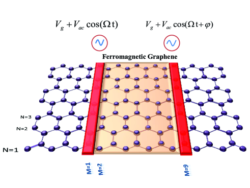
As shown in Fig.1, we consider zigzag graphene nanoribbon in the proximity of ferromagnetic insulator such as $EuO$ Haugen and yttrium iron garnet (YIG)PRL2015 which is connected to two infinite electrodes. For simplicity, the electrodes are considered to be the same nanoribbon as the central system. One $\pi$ orbital is considered per each site for graphene system. So the single electron Hamiltonian of the central region is described as

$$\begin{array}[]{r}H^{\sigma}_{C}(t)=\sum_{i\sigma}(\varepsilon^{C}_{i}(t)-\sigma h)c^{\dagger}_{i\sigma}c_{i\sigma}+\\ \sum_{<ij>\sigma}t_{0}(c^{\dagger}_{i\sigma}c_{j\sigma}+c_{i\sigma}c^{\dagger}_{j\sigma})\end{array}$$ (1)

.

where $c^{\dagger}_{i\sigma}$ and $c_{i\sigma}$ are the electron creation and annihilation operators and $t_{0}$ is the hopping energy between nearest neighbour atoms, respectively. All energies are scaled in unit $t_{0}$. $\sigma=\pm 1$ refers to up and down-spin. Here $h$ is the induced exchange field arising from strong proximity of a ferromagnetic insulator. This induced exchange field can be tuned by means of an in-plane external electric field ex-tune . The exchange splitting inducing by a ferromagnetic insulator such as $Euo$ in graphene has been estimated to be in the range of $5-65meV$Haugen ; semenov ; PRL2015 . The coupling Hamiltonian which is independent of time is defined as the following: $H_{coupling}=\sum_{<ij>}(t_{LC}c^{\dagger}_{i}c_{j}+t_{RC}c_{i}c^{\dagger}_{j})+H.c.$, where $t_{LC}$ and $t_{RC}$ are the coupling energy between the electrodes and central ribbon. To have quantum pumping, one should break left-right symmetry by application of a dynamic or static asymmetric spatial factor. Here, we will apply a dynamical break of the left-right symmetry appearing as a phase lag between two oscillating gate voltages. Therefore, in the case of static symmetry such as $t_{LC}=t_{RC}$, one can still observe $dc$ pumped current. Harmonically time-dependent gate voltages are applied just on the last and first atomic layers of the central region as shown in Fig.1.

$$\begin{array}[]{r}\varepsilon^{C}_{i}(t)=eV^{g}_{i}+eV^{ac}_{i}cos(\Omega t+\varphi_{i})\end{array}$$ (2)

.

where $V^{ac}_{i}$ and $\Omega$ are the strength and frequency of the oscillating gate voltages, respectively. Moreover, let us apply zero gate voltage on all sites $V^{g}_{i}=0$, except the first and last unit cells that include two barriers as strong as $V^{g}_{i}=1$. Constant gate voltage causes to shift Van Hove singularities into the band center giving rise an enhanced pump currentFoa-APL2011 . To break the left-right symmetry, as shown in Fig.1, two $ac$ gate voltages with a phase lag $\varphi=\varphi_{R}-\varphi_{L}$ are applied on the first ($\varphi_{L}=0$) and last ($\varphi_{R}=\varphi$) unit cells along the transport direction. We consider the phase difference between two $ac$ gate voltages to be $\varphi=\pi/2$ in which the maximum $dc$ current has been reported in quasi-one dimensional systemsMoskalets ; Arrachea ; Arrachea2012 . Two semi-infinite electrodes are not driven by any time-dependent gate voltages. Because of zero source-drain voltage, we set on-site energies of the electrodes to be zero.

To obtain $dc$ current through graphene nanoribbon, we use a Floquet theory in combination with non-equilibrium Green’s function formalism. It should be noted that the electron-electron interaction is not considered in this calculation. At zero temperature, the averaged pump current over one period of the $ac$ gate voltage for spin $\sigma$ is written as the followingkohler ; kitagawa ; Foa .

$$\begin{array}[]{r}\overline{I}_{\sigma}=\frac{e}{h}\sum_{n}\int_{-\infty}^{E_{F}}d\varepsilon T^{n}_{\sigma}(\varepsilon)\end{array}$$ (3)

where

$$T^{n}_{\sigma}(\varepsilon)=T_{RL,\sigma}^{n}(\varepsilon)-T_{LR,\sigma}^{n}(\varepsilon)$$

and $E_{F}$ is the Fermi energy. The transmission probability of carriers coming from the left to the right electrode $T_{RL,\sigma}^{n}(\varepsilon)$ assisted by the absorption ($n>0$) or emission ($n<0$) of $\mid n\mid$ photons with an incident energy of carriers $\varepsilon$ and spin $\sigma$ can be written in terms of Floquet Green’s function $G_{\sigma}^{n}(\varepsilon)$ as the following.

$$\begin{array}[]{r}T_{RL\sigma}^{n}(\varepsilon)=Tr[\Gamma^{\sigma}_{R,n}(\varepsilon)G_{RL,\sigma}(\varepsilon)\Gamma^{\sigma}_{L,0}(\varepsilon)G_{RL,\sigma}^{\dagger}(\varepsilon)]\end{array}$$ (4)

where Floquet Green’s fucntion is calculated in based on the Floquet states as $G_{RL,\sigma}^{n}(\varepsilon)=\langle R,n|(\varepsilon I-H_{F})^{-1}|L,0\rangle$ and Floquet Hamiltonian is defined as $H_{F}=H_{C}(t)-i\hbar\frac{\partial}{\partial t}$. The Floquet Green’s function is a Fourier transformation of retarded Green’s function as the following:

$$G_{RL,\sigma}^{r}(t,\varepsilon)=\sum_{n=-\infty}^{\infty}G_{RL,\sigma}^{n}(\varepsilon)\exp(-in\Omega t).$$

Taking Fourier transform of the equation of motion governing on the retarded Green’s function results in an equation of motion followed by the Floquet Green’s function. The escape rates of electrons to the electrodes through elastic or inelastic channels are defined as the following.

$$\Gamma_{\alpha,n}(\varepsilon)=i[\Sigma_{\alpha}(\varepsilon+n\hbar\omega)-\Sigma^{{\dagger}}_{\alpha}(\varepsilon+n\hbar\omega)]$$

where the index $n$ shows the number of photons assisted for inelastic transport and $\Sigma_{\alpha}(\varepsilon)$ is the Floquet self energy arising from the electrodes $\alpha=L,R$. In the calculations, the convergence of the transmission functions determines the number of required Floquet channels $n$. In the case of non-interacting systems, the above formalism is equivalent to non-equilibrium Green’s function formalism (Keldysh formalism)Arrachea-moskalet .

Figure 2: Pumped current in terms of driving frequency at the band center $E=0$ for ZGNR(12,4). Blue solid line (red dash-dot line) shows charge (spin) pumped current. In the lower panels, some of frequency’s ranges are magnified to present some special frequencies.

III Results

III.1 Driving Frequency Dependence of Pumped Current

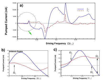
We present in Fig.2 the results for spin and charge pumped current through zigzag graphene nanoribbons as a function of driving frequency $\Omega$ at the band center. The charge and spin pumped current are defined as $I_{C}=I_{\uparrow}+I_{\downarrow}$ and $I_{S}=I_{\uparrow}-I_{\downarrow}$, respectively. $I_{\uparrow}$ and $I_{\downarrow}$ refer to the up and down spin currents. For very low frequencies (adiabatic regime), there is a linear behavior of charge pumped current in terms of $\Omega$ which is in compatible with the results reported beforepump-GNR . This linear behavior which is shown in Fig.(2.b), is a character of the adiabatic pumpingBrouwer . However, close to the Van Hov singularities, the scale of pumped current with the frequency is improvedFoa-APL2011 .

The characteristic energy scale in this system is defined as $n_{max}*\Omega$ in which $n_{max}$ is the maximum number of sidebands excited by the driving gate voltages. The adiabatic regime occurs when this energy scale is small enough in compared to the level spacing of the resonant states. On the other hand, $n_{max}$ depends on the ratio of $V_{ac}/\Omega$. It means that the adiabatic regime occurs at lower frequencies when the strength of pumping is large. Furthermore, longer or wider ribbons result in smaller level spacing. Therefore, larger pumps have smaller frequency ceiling for working in the adiabatic regime. The adiabatic regime is indicated by the point $1$ in Fig.(2.b) which corresponds to the pumping frequency as small as $\Omega_{1}=0.01t_{0}$. Although the level spacing is energy dependent, in our system, one can estimate it to be about $0.2$ ($t_{0}$) which is larger than $\Omega=0.01(t_{0})$. In the adiabatic regime, spin pumping is small, however there is no pure spin pumping in this regime.

At high frequency regime, spin and charge pumped current show some extremum points at the special values of the driving frequencies which are originated from the resonance of the Floquet states with those atomic levels captured between two barriers. Therefore one can control the direction and amplitude of the spin current by tuning the driving frequency. At frequencies that are multiples of the level spacing, by mediated of photon-assisted transitions, atomic levels are mixed with each other. Therefore, an enhanced pumped current emerges in this situation. However, level spacing is not uniform along the whole spectrum, so an interplay between driving frequency and level spacing is more complicated.

In the non-adiabatic regime, spin-polarized pumped current is observable along the whole range of driving frequencies shown in Fig.(2). However, full spin polarized pumping are categorized in the following three interesting cases: i) in the case of $I_{C}=I_{S}$, there exists pure up-spin polarized current. So we have $I_{\uparrow}\neq 0,I_{\downarrow}=0$. This case is marked by the point $2$ in Fig.(2) referring to $\Omega_{2}$. If charge and spin pumped current are positive/negative, up-spin current is pumped from the left/right to the right/left electrode. ii) The case of $I_{C}=0$ which emerges at the frequency $\Omega_{3}$, results in a fully spin pumping with zero net charge pumping. The pumped currents for up and down spins are in the opposite directions $I_{\uparrow}=-I_{\downarrow}$.

In fact, quantum interference is responsible for such interesting cases. In the adiabatic regime, pumped current is an odd function of the phase difference between oscillating gate voltages. However, in the non-adiabatic regime, an additional contribution to the phase difference is originating from the spatial phase difference of the Floquet sidebandsMoskalets . This phase difference which is absent at low frequency regime, is responsible for the sign reversal of the pumped current at consecutive peaks shown in Fig.2. Photon-assisted Quantum interference through different Floquet side-bands can result in a special case; two spin-polarized pumped current which flow in the opposite directions. So in this case, there is no net charge pumping while it is purely spin-polarized pumping in the opposite directions.

iii) Correspondingly, the case of $I_{C}=-I_{S}$ also results in a fully down-spin polarized currents $I_{\uparrow}=0,I_{\downarrow}\neq 0$. If $I_{C}>0$, then we have $I_{\downarrow}>0$. This frequency is indicated by $\Omega_{4}$. In other cases, the pumped current is partially spin polarized. Spin polarization emerges when the density of state for up and down spins shift against each other, so at a given frequency, level spacing for up spins differs from one for down spins. As a consequence, pumped current for up and down spin would be different in its value and also pumping direction. Moreover the effect of higher orders of the orbital overlaps on the pumped current is investigated in the Appendix.

III.2 Fermi Energy Dependence of Pumped Current

Let us concentrate on the Fermi energy dependence of the pumped current at these four special driving frequencies shown in Fig.3. Panel (a) in Fig.3 shows spin-up and down pumped current as a function of Fermi energy for small pumping frequency $\Omega_{1}=0.01t_{0}$. This frequency is smaller than two consecutive energy levels of the central region. The pumped current contains successive small peaks which are modulated on a pumped currentFoa-APL2011 . These peaks in the pumped current are originated from the peak-antipeak structureArrachea of the net pumped transmission ($\sum_{n}T^{n}_{\sigma}$) shown in Fig.(4.a). In this regime, there is no mixing between system levels, therefore spin polarization is small. However, there exists unidirectional charge pumping along the whole range of Fermi energies.

Figure 3: Pumped current in terms of Fermi energy for ZGNR(12,4) at the specified driving frequencies of $\Omega_{1},\Omega_{2},\Omega_{3},\Omega_{4}$ which have been marked in Fig.2.

Panels (b), (c) and (d) in Fig.3 indicate fully spin polarized pumped current in terms of Fermi energy for the frequencies $\Omega_{2},\Omega_{3},\Omega_{4}$. Apparently, because of two barriers applied on the first and last unit cells, electron-hole symmetry breaks. Furthermore, the pumped current increases around $E=-1$ which is in resonance with the barriers. In panel (b) and at $\Omega_{2}$, down-spin current is blocked and up-spin is fully pumped from the right to the left electrode. At $\Omega_{3}$ and in the panel (c), we present an interesting case of pure spin current with zero net charge pumping over a wide range of Fermi energy around the band center. Finally, at the frequency $\Omega_{4}$, down-spin is fully pumped, while up-spin is still blocked. There is some structure of jumps and plateaus in panels (b) to (d) which follow the resonant states shown in the net pumped transmission curve (Fig.4b,c). The behavior of pumped current in ZGNRs is similar to the pumped current passing through one-dimensional chainArrachea .

Fig.(4) shows the net pumped transmission curve (which is defined as $\sum_{n}T^{n}_{\sigma}(\varepsilon)$) as a function of energy for different driving frequencies. For low driving frequency $\Omega_{1}$, peaks and anti-peaks in the net transmission curve emerge around the resonant states located between two barriers (Fig.(4.a)). At both energies of peak and anti-peak, we observe large quantum pumping and hence constructive interference. On each peak-antipeak pattern, at lower energies, the left to the right pumping is dominant while at higher energies, pumping direction will be from the right to the left side. The following adiabatic picture may be useful to understand the reason for such behavior: At half period of oscillating potential, the left barrier has a lower gate voltage in compared to the right barrier. So electrons flow from the right reservoir into the well. In the other half of period, the right barrier gets lower which leads to a current flow from the well into the right reservoir. If we turn off the oscillating gates, transmission would have peaks at the resonant states as the original transporting channels.

Figure 4: Net pumped transmission in terms of Fermi energy for ZGNR(12,4) at the specified driving frequencies of $\Omega_{1},\Omega_{2},\Omega_{3}$ which have been marked in Fig.2. The norm of the left-right green’s function for single photon-assisted transmission is plotted in part (b) for the low frequency regime $\Omega_{1}$.

At low frequency regime, there is no mixing between system levels, so transport occurs mainly through resonant and also one Floquet side state. However, at high frequencies, the system levels are mixed with each other arising from the driven potential. As a result, large peaks are appeared in the net pumped transmission which are observed in Figs.(4.b,c).

III.3 Practical Implementations

In reality and in the absence of coulomb blockade, stray capacitances between the gates and electron reservoirs may affect adiabatic quantum pumping in the work done by SwitkesSwitkes . However, some features of the observed dc voltage are in agreement with the theoretical calculations based on the scattering matrixBrouwer2001 . To have conclusive spin pumping, one of the powerful techniques is precessing magnetization at ambient temperaturebauer-RMP . Furthermore, the other technique is the use of the ac Josephson effect in a hybrid normal-superconducting system russo or charge pumping in an unbiased InAs nanowire embedded on a superconductornature-josephson . For graphene nanoribbons with smooth edges, in the adiabatic regime, it is expected to observe some general feature of quantum pumps at low temperatures. Furthermore, we have shown beforecheraghchi that in graphene nanoribbons, under application of a weak source-drain voltage, screening effects are weak. Therefore, in a weak driving gate voltages, accumulation and depletion of charge would be small. On the other hand, homogeneity of the junctions reduce stray capacitances between oscillating gates and electron reservoirs. Here we assume that the electrodes are similar to the pumping region for having transparent contacts in compared to the normal pumps.

In reality, the width of nanoribbons are much wider than what we have considered in this paper. Wider and longer nanoribbons have smaller energy level spacing. So it is expected that for wider and longer nanoribbons, more sign reversal happens for the pumped current curve in terms of the driving frequency. For graphene sheet, there exists pure spin pumping at special energies in the adiabatic regimezhang . Pure spin pumping is also expected to observe in wider graphene nanoribbons.

During fabrication processes, the ribbons are full of impurity or disorder. So we propose to investigate the effect of disorder and impurity locations on the pure spin and charge pumping through graphene nanostructures.

IV Conclusion

In conclusion, we study charge and spin pumping in ferromagnetic graphene nanoribbons including a double-barrier structure driven weakly by two local ac gate voltages with a phase-lag. With new improvements to induce exchange magnetic field in graphene PRL2015 , the main point of this paper is that charge and spin pumping can be well controlled by tuning the driving frequency in the non-adiabatic regime. Furthermore, fully spin pumping with favorite direction is achievable at the special frequency of ac gate voltages. It seems that at low frequency regime, single photon-assisted tunneling is dominant, while at higher frequencies, mixing of energy levels arising from the driving field leads to constructive interference.

Figure 5: Spin pumped current ($I_{S}$) as a function of driving frequency for ZGNR(20,4) at the band center for two cases: a) by considering of the nearest neighbor overlaps (NN-GNR), b) the second and third nearest neighbor hopping energies (3NN-GNR).

V Acknowledgement

We gratefully acknowledge Luis E. F. Foa Torres for his useful comments during improvement of this work. HC thanks the International Center for Theoretical Physics (ICTP) for their hospitality and support during a visit in which part of this work was done.

VI Appendix

VI.1 Higher order orbital overlaps

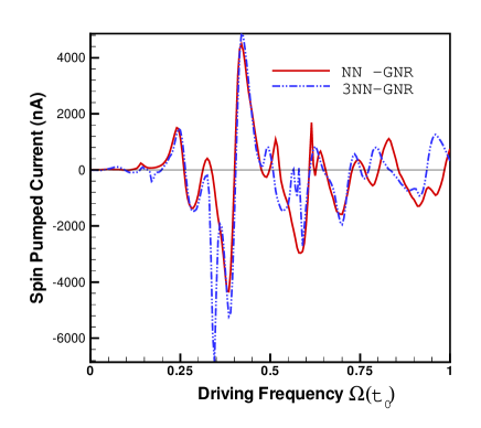
In the tight binding model shown in equation 1, hamiltonian contains nearest neighbor interaction. However, ab initio band structures can be extracted by considering of the second and third nearest neighbor overlaps in Hamiltonian. To investigate the effect of higher order overlaps, the pumped current is calculated by using tight-binding parameters which are proposed by Ref.(Riech, ). The distances between the first, second and third nearest neighbors are given by $a_{1}=1.42{\hat{A}},a_{2}=\sqrt{3}a_{1},a_{3}=2a_{1}$. The values of nearest-neighbor hopping parameters are calculated by comparing and fitting the first principle and tight-binding band structures for different types of grapheneRoche (2D graphene, graphene nanoribbons and nanotubes ). The second and third hopping parameters are considered as $0.12eV$ and $0.068eV$ if the nearest-neighbor hopping $t_{0}$ is considered to be as $2.78eV$Riech .

Fig.5 shows spin pumped current ($I_{S}$) in terms of driving frequency for the two cases: Considering of a)the nearest neighbor overlap (NN-GNR), b) the second and third nearest neighbor overlap (3NN-GNR). As it is shown, spin pumped current shows more extremum for the 3NN-GNR case in compared to the NN-GNR case.

References

- (1) P. W. Brouwer, Phys. Rev. B. 58, 135 (1998).
- (2) M. Switkes, et al., Science, 283, 1905 (1999).
- (3) S. Kohler, J. Lehmann, and P. Hanggi, Phys. Rep. 406, 379 (2005).
- (4) E. R. Mucciolo, C. Chamon, and C. M. Marcus, Phys. Rev. Lett. 89, 146802 (2002); L. DiCarlo and C. M. Marcus, J. S. Harris, Phys. Rev. Lett. 91, 246804 (2003); S. K. Watson, R. M. Potok, C. M. Marcus, and V. Umansky, Phys. Rev. Lett. 91, 258301 (2003); ibid, Phys. Rev. Lett. 91, 258301 (2003).
- (5) D. Huertas-Hernando, F. Guinea, and A. Brataas, Phys. Rev. B. 74, 155426 (2006); Hongki Min, J. E. Hill, N. A. Sinitsyn, B. R. Sahu, L. Kleinman, and A. H. MacDonald, Phys. Rev. B. 74, 165310 (2006); Y. Yao, F. Ye, X. L. Qi, S. C. Zhang, and Z. Fang, Phys. Rev. B. 75, 041401, (2007).
- (6) N. Tombros, C. Jozsa, M. Popinciuc, H. T. Jonkman, B. J. van. Wees, Nature, 448, 571 (2007).
- (7) H. cheraghchi, F Adinehvand, J. Phys: Condens. Matter. 24, 045303 (2012); V. Derakhshan, H. Cheraghchi, J. Magn. Mater. 357, 29 (2014).
- (8) Q. Zhang, K. S. Chan, and Z. Lin, Appl. Phys. Lett. 98, 032106 (2011).
- (9) H. Haugen, D. Huertas-Hernando, A. Brataas, Phys. Rev. B. 77, 115406 (2008).
- (10) Z. Wang, C. Tang, R. Sachs, Y. Barlas, and J. Shi, Phys. Rev. Lett. 114, 016603 (2015).
- (11) A. H. Castro Neto, et al., Rev. Mod. Phys. 81, 109 (2009).
- (12) E. Prada, P. San-Jose, and H. Schomerus, Phys. Rev. B. 80, 245414 (2009). E. Prada, P. San-Jose, and H. Schomerus, Solid State Comm. 151, 1065 (2011); P. San-Jose, E. Prada, S. Kohler, and H. Schomerus, Phys. Rev. B. 84, 155408 (2011).
- (13) G. M. M. Wakker and M. Blaauboer, Phys. Rev. B. 82, 205432 (2010).
- (14) Y. Gu, Y. H. Yang, J. Wang,and K. S. Chan, J. Phys.: Condens. Matter. 21, 405301 (2009).
- (15) E. Grichuk and E. Manykin, Euro. Phys. Lett. 92, 47010 (2010); ibid, JETP Letters, 93, 372 (2011).
- (16) T. Kaur, L. Arrachea, and N. Sandler, arXiv:1203.3952 (2012).
- (17) Y. Zhou and M. W. Wu, Phys. Rev. B. 86, 085406 (2012).
- (18) C. G. Rocha, L. E. F. Foa Torres, and Gianaurelio Cuniberti, Phys. Rev. B. 81, 115435 (2010).
- (19) L. E. F. Foa Torres, H. L. Calvo, C. G. Rocha, and G. Cuniberti, Appl. Phys. Lett. 99, 092102 (2011).
- (20) M. Moskalets and M. Buttiker, Phys. Rev. B. 66, 205320 (2002).
- (21) B. Wang, J. Wang, and H. Guo, Phys. Rev. B. 65, 073306 (2002).
- (22) L. Arrachea, Phys. Rev. B. 72, 125349 (2005).
- (23) M. M. Mahmoodian, L. S. Braginsky, and M. V. Entin, Phys. Rev. B. 74, 125317 (2006).
- (24) E. Faizabadi, Phys. Rev. B. 76, 075307 (2007); E. Faizabadi and F. Ebrahimi, J. Phys.: Condens. Matter 16, 1789 (2004).
- (25) M. Moskalets, and M. Bttiker, Phys. Rev. B. 78 035301 (2008).
- (26) T. Kitagawa, T. Oka, A. Brataas, L. Fu, and E. Demler, Phys. Rev. B. 84, 235108 (2011).
- (27) L. E. F. Foa Torres, Phys. Rev. B. 72, 245339 (2005).
- (28) L. Arrachea, M. Moskalets, Phys. Rev. B. 74, 245322 (2006).
- (29) E.-J. Kan, Z. Li, J. Yang and J. G. Hou, Appl. Phys. Lett. 91, 243116 (2007)); S. Dutta and S. K. Pati, J. Phys. Chem. B. 112, 1333 (2008).
- (30) Y. G. Semenov, J. M. Zavada, and K. W. Kim, Phys. Rev. B. 77, 235415 (2008).
- (31) P. W. Brouwer, Phys. Rev. B 63, 121303(R) (2001).
- (32) Y. Tserkovnyak, A. Brataas, G. E. W. Bauer, and B. I. Halperin, Rev. Mod. Phys. 77, 1375 (2005).
- (33) F. Giazotto, et. al., Nature Physics 7, 857 (2011).
- (34) S. Russo, et. al, Phys. Rev. Lett. 99, 086601 (2007).
- (35) H. Esmailzadeh, H. Cheraghchi, Nanotechnology, 21, 205306 (2010).
- (36) S. Riech, et. al., Phys. Rev. B. 66, 035412 (2002).
- (37) A. Cresti, et. al, Nano. Res. 1, 361-394 (2008).