Observational Evidences of Electron-driven Evaporation in two Solar Flares

Abstract

We have explored the relationship between hard X-ray (HXR) emissions and Doppler velocities caused by the chromospheric evaporation in two X1.6 class solar flares on 2014 September 10 and October 22, respectively. Both events display double ribbons and Interface Region Imaging Spectrograph (IRIS) slit is fixed on one of their ribbons from the flare onset. The explosive evaporations are detected in these two flares. The coronal line of Fe XXI 1354.09 Å shows blue shifts, but chromospheric line of C I 1354.29 Å shows red shifts during the impulsive phase. The chromospheric evaporation tends to appear at the front of flare ribbon. Both Fe XXI and C I display their Doppler velocities with a ‘increase-peak-decrease’ pattern which is well related to the ‘rising-maximum-decay’ phase of HXR emissions. Such anti-correlation between HXR emissions and Fe XXI Doppler shifts, and correlation with C I Doppler shifts indicate the electron-driven evaporation in these two flares.

1 Introduction

Solar flares are drastic explosive phenomena on the Sun. They are able to release a huge amount of energy ($\sim$10³² erg) in a typical time scale of tens of minutes. Based on the standard model, the flare energy is transferred from the magnetic energy. Magnetic reconnection is thought to be the primary energy release mechanism that heats the plasmas and accelerates the bi-directional nonthermal electrons in the solar atmosphere. This is known as the CSHKP model (Carmichael, 1964; Sturrock, 1966; Hirayama, 1974; Kopp & Pneuman, 1976). These nonthermal electrons which guided by the reconnected magnetic field lines, not only travel to the interplanetary space but also precipitate into the lower corona and upper chromosphere, where they lose energy to produce radiation through Coulomb collisions with the denser medium. This has been known as the ‘thick-target’ model for the hard X-ray (HXR) emission (Brown, 1971; Syrovatskii & Shmeleva, 1972). Observations show that only a small fraction of the energy is lost through extreme-ultraviolet (EUV) radiation (Emslie et al., 1978; Milligan et al., 2014; Milligan, 2015). The bulk of the energy heats the local chromospheric material rapidly up to a typical temperature of $\sim$10 MK. Then the resulting overpressure can drive the mass flow upward along the loop at speeds of a few hundreds kilometers per second. The hot plasmas fill the flaring loops in a process called ‘chromospheric evaporation’ (Brown, 1973; Acton et al., 1982; Fisher et al., 1985a, b; Liu et al., 2006; Ning et al., 2009; Ning & Cao, 2010; Zhang & Ji, 2013; Milligan, 2015), resulting into soft X-ray (SXR) emission rising up. Substantial evidences of chromospheric evaporation have been reported in X-ray (e.g., Liu et al., 2006; Ning et al., 2009; Ning & Cao, 2010; Ning, 2011; Ning & Cao, 2011; Nitta et al., 2012; Zhang & Ji, 2013), EUV (e.g., Doschek et al., 1980; Feldman et al., 1980; Antonucci et al., 1982; Ding et al., 1996; Teriaca et al., 2006; Milligan et al., 2006a, b; Milligan & Dennis, 2009; Veronig et al., 2010; Chen & Ding, 2010; Li & Ding, 2011; Doschek et al., 2013; Brosius, 2013) and radio (Aschwanden & Benz, 1995; Karlicky, 1998; Ning et al., 2009) emissions. Previous observations reveal that HXR emission tends to rise with the double footpoint sources along the flaring loop legs, eventually merging them into a single source at the same position of the loop-top source (Liu et al., 2006; Ji et al., 2007, 2008; Ning et al., 2009; Ning & Cao, 2010; Ning, 2011; Ning & Cao, 2011). This is because the dense materials from the chromosphere rise upward along the loops, following the movement of the HXR emission targets. The flare shows the mergence speed of around 200 km s^-1. Such large value of the mass evaporation is clearly demonstrated by the blue shifts at the EUV spectral observations of the coronal lines (Feldman et al., 1980; Ding et al., 1996; Berlicki et al., 2005; Teriaca et al., 2006; Brosius & Holman, 2007; Milligan & Dennis, 2009; Veronig et al., 2010; Chen & Ding, 2010; Li & Ding, 2011; Doschek et al., 2013; Brosius, 2013; Tian et al., 2014a; Young et al., 2015). Spectral images exhibit that the blue shifts tend to appear at the outsides of the flare ribbons (Czaykowska, 1999; Li & Ding, 2004). Evaporation materials with high temperature rise upward to disturb the coronal plasma, which results into the radio emission suddenly suppressed on the radio dynamic spectra, especially at the decimeter range. A high-frequency cutoff drifting to lower frequency is thought to be the signature of chromospheric evaporation (Aschwanden & Benz, 1995; Karlicky, 1998; Ning et al., 2009)

From the observations, there are two types of chromospheric evaporation. Evaporation is said to proceed ‘gently’ when the chromosphere plasmas lose energy via a combination of radiation and low-velocity hydrodynamic expansion. Emission lines formed at temperature characteristic of the atmosphere from chromosphere through transition region to corona all appear blue shifted (Milligan et al., 2006b; Brosius, 2009; Raftery et al., 2009; Li & Ding, 2011). Evaporation is regarded to proceed ‘explosively’ when the chromosphere is unable to radiate energy at a sufficient rate and consequently expands at high velocities into the overlying flare loops. The overpressure of evaporated material also drives low-velocity downward motion into the underlying chromosphere, in a process known as ‘chromospheric condensation’ (Wülser et al., 1994; Czaykowska, 1999; Kamio et al., 2005; Del Zanna et al., 2006; Teriaca et al., 2006). In this case, emission lines formed at temperature characteristic of the upper chromosphere and transition region all appear red shifted, while hotter lines from the corona appear blue shifted (Fisher et al., 1985a, b; Milligan et al., 2006a; Del Zanna et al., 2006; Brosius, 2009; Raftery et al., 2009; Li & Ding, 2011). Spectral observations show the red shifted velocity of $\sim$20 to 40 km s^-1, which is an order smaller than the blue shifted value ($\sim$200 km s^-1). This is because the plasma density of the underlying lower chromosphere is much higher than that of the overlying corona.

Up to now, there are two viewpoints about how to drive the evaporation in the literatures. One is the electron-driven, while another is the thermal conduction driven. The former emphases that the non-thermal energy of nonthermal electrons play an important role in the evaporation (Fisher et al., 1985a, b; Milligan & Dennis, 2009; Tian et al., 2014a), while the latter focuses on the thermal energy directly driven (Fisher et al., 1985a; Falewicz et al., 2009). In this paper, using the observations from Fermi Gamma-ray Burst Monitor (GBM), Reuven Ramaty High Energy Solar Spectroscopic Imager (RHESSI), Atmospheric Imaging Assembly (AIA) aboard Solar Dynamics Observatory (SDO) and Interface Region Imaging Spectrograph (IRIS), we explore the relationship between HXR emissions and Doppler velocities caused by evaporation during the impulsive phase in two solar flares in order to detect the observation evidences of the electron-driven chromospheric evaporation.

2 Observations and Data Analysis

2.1 Observations

Two X1.6 solar flares are selected to study in this paper. Firstly they are well covered by the IRIS (De Pontieu et al., 2014) spectral observations. IRIS slit is fixed on the flare ribbon during the impulsive phase, which gives us an opportunity to detect the whole history of Doppler velocities caused by evaporation. Secondly, HXR emissions are also well observed by Fermi (Meegan et al., 2009) or RHESSI (Lin et al., 2002). One event takes place in NOAA AR 12158 on 2014 September 10. It starts at 17:21 UT and reaches its maximum at 17:45 UT on the GOES SXR light curves. Another occurs in NOAA AR 12192 on 2014 October 22. It starts at 14:02 UT and peaks at 14:28 UT on the SXR emissions.

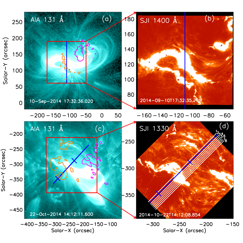
Figure 1: Top: AIA 131 Å (a) and SJ 1400 Å (b) images at 17:32 UT on 2014 September 10. Bottom: AIA 131 Å (c) and SJ 1330 Å (d) images at 14:12 UT on 2014 October 22. The blue and white lines represent the IRIS slit positions. The contours indicate the magnetic fields from HMI at the levels of 800 (purple) and -800 (orange) G. The red boxes mark the IRIS SJI regions. Two short blue lines on the IRIS slit in panels (c, d) mark the flare ribbon shown in Fig. 6.

Fig. 1 shows the SDO/AIA (Lemen et al., 2012) 131 Å images (a, c) and IRIS/SJ images (b, d) of these two flares. The contours on the AIA 131 Å images represent the line-of-sight magnetic fields from Helioseismic and Magnetic Imager (HMI) (Schou et al., 2012) aboard SDO. The levels are set at 800 (purple) and -800 (orange) G, respectively. IRIS slit is fixed along the solar North-South direction on one ribbon of 2014 September 10 flare. The cadence is 9.4 s. For the 2014 October 22 flare, IRIS slit is along the 45 degree to the North-South direction. IRIS detects the flare ribbon in the ‘raster’ mode. Each raster has eight steps (marked by the number on the SJI 1330 Å image). Each step has a cadence of 16.4 s and a distance of $\sim$2″. Thus each raster has a duration of $\sim$131 s.

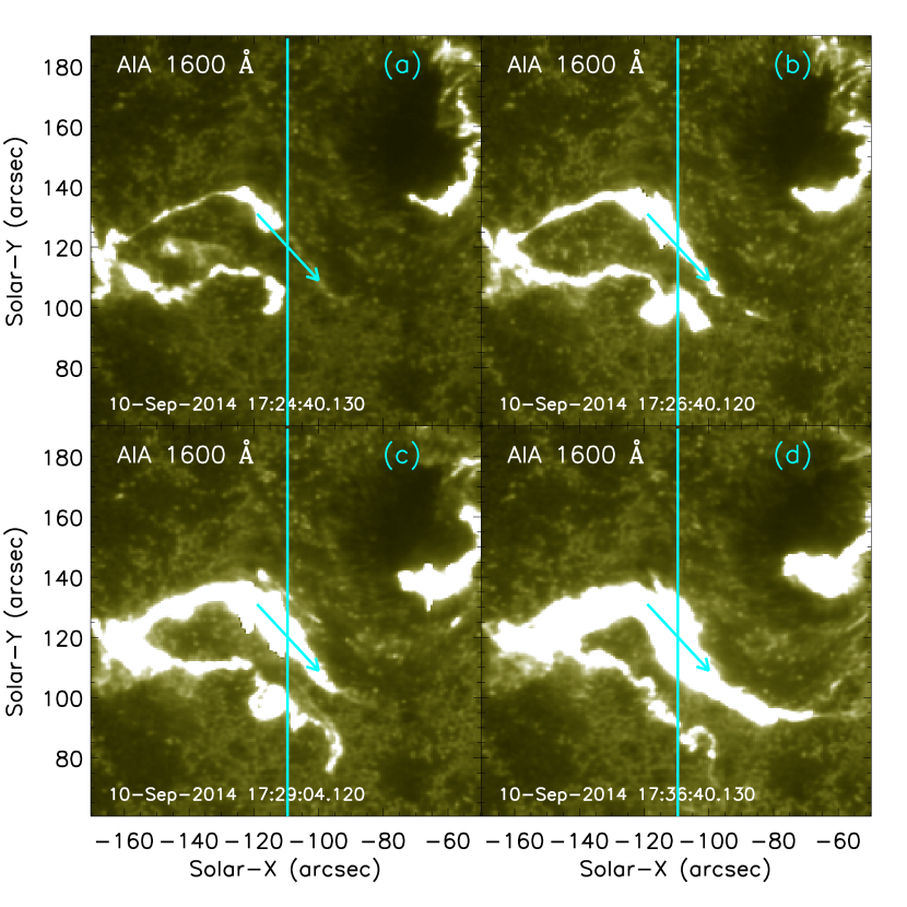
Figure 2: Time sequences of AIA 1600 Å images for the 2014 September 10 flare. The vertical line represents the IRIS slit positions, and the arrows mark the ribbon propagation.

Both events display the double ribbons at SJI 1400 Å or 1330 Å images, as shown in Fig. 1 (b, d). The 2014 September 10 flare shows one short ribbon around the positive filed region, while another is long with a curved shape around the negative filed region. This long ribbon is dynamic and propagating toward the South-East direction, subsequently crosses the IRIS slit during the flare impulsive phase. Fig. 2 gives the time evolution of this ribbon on AIA 1600 Å images. The arrow marks the ribbon propagation direction. This ribbon also exhibits strong Quasi-Periodic Pulsations (i.e., Li & Zhang, 2015; Li et al., 2015). Similar to the 2014 September 10 flare, one ribbon of the 2014 October 22 flare is around the positive filed region, and the other ribbon at the negative filed region is detected by the IRIS slit during the flare impulsive phase.

2.2 Spectral fitting

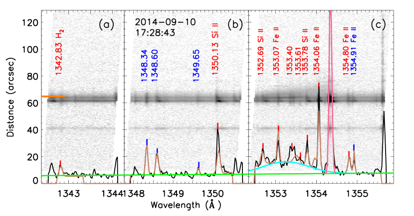
Figure 3: Three IRIS spectra windows ((a) for ‘1343’, (b) for ‘Fe XII ’, and (c) for ‘O I ’) at 17:28:43 UT for 2014 September 10 flare. The black profiles are detected at $\sim$64.7″ along the slit positions (marked by the short horizontal line). The brown profiles represent the multi-Gaussian fitting. The turquoise profile is Fe XXI , the magenta profile is C I , and the green is the background. The other 13 emission lines used in this paper are labeled by vertical ticks.

Fig. 3 shows the IRIS spectral profiles of three windows at ‘1343’ (a), ‘Fe XII ’ (b), and ‘O I ’ (c) for the 2014 September 10 flare. IRIS has a spectral scale of $\sim$25.6 mÅ/pixel for these three windows. The spectral data has been firstly calibrated and processed with the routines of iris_orbitvar_corr_l2.pro and iris_prep_despike.pro in the solar software (SSW) package. The first routine is used to correct IRIS spectral image deformation caused by the spacecraft orbital variation (Tian et al., 2014b; Cheng et al., 2015). The second one is a generalized despiking tool for IRIS data. It could identify and remove the bad pixels through the iterative approach. At the flare onset (i.e., 17:28:43 UT), the spectral window at ‘O I ’ is characterized by many narrow, bright emission lines from neutral and singly ionized species, as well as molecular fluorescence lines. These emission lines blend with the broad line of Fe XXI 1354.09 Å (seen also., Li et al., 2015; Polito et al., 2015; Tian et al., 2014a, 2015; Young et al., 2015), which is a typical coronal line to be used to detect the chromospheric evaporation. However, these blending chromospheric emission lines must be extracted before determining the Fe XXI intensity. According to the characteristics of IRIS spectral data, three steps are followed.

Firstly, to determine the line centers and widths (FWHM: the full width at half maximum) at ‘O I ’ window, including blending lines and Fe XXI . There are seven blending lines of Fe XXI , including Fe II 1353.07, 1354.06 Å, Si II 1352.69, 1353.78 Å, C I 1354.29 Å, and two unidentified lines at 1353.40, 1353.61 Å, such as marked by the red vertical ticks (except for C I ) in Fig. 3 (c). These lines are bright in the active regions while Fe XXI is quiet. Therefore, their line centers and widths can be detected from the single-Gaussian fitting in the active regions. During the solar flare, their centers and widths are constrained in a range to do spectral fitting based on the previous observations (e.g., Curdt et al., 2001, 2004). Taking the emission line of Si II 1352.69 Å for example, its center and width during the flare are same as the values from the active regions but constrained, such as line center at 1352.69$\pm$0.102 Å (ranging from 1352.588 to 1352.792 Å), and the maximum width of 260 mÅ, as listed in table 1. C I has the strongest emission among these seven lines. Previous studies (Doschek et al., 1975; Cheng et al., 1979; Mason et al., 1986; Innes et al., 2003a, b) have identified its rest wavelength at 1354.29 Å and its narrow width, which is assumed with maximum value of 130 mÅ for the flare spectral fitting in this paper. Its line center is set at the range of 1354.29$\pm$0.26 Å for the flare spectral fitting. Based on the fact that Fe XXI is a broad line (see., Doschek et al., 1975; Cheng et al., 1979; Mason et al., 1986; Innes et al., 2003a, b; Tian et al., 2014a, 2015; Li et al., 2015). Its line center is set as 1354.29$\pm$1.28 Å, which almost cover the whole ‘O I ’ window, and its line width is assumed with a minimum value of 230 mÅ, as listed in Table 1.

Secondly, to tie the blending line intensities from other similar isolated lines during the flare. Fig. 3 (c) shows coronal line of Fe XXI 1354.29 Å blending with these seven emission lines for the 2014 September 10 flare. There is no way to determine their flare intensities only at ‘O I ’ window. However, IRIS has the spectra at other windows, i.e., ‘1343’, ‘Fe XII ’. They also have the emission lines which behave similarly to the blending lines at ‘O I ’ window, such as H₂ 1342.83 Å at ‘1343’ window, Si II 1350.13 Å at ‘Fe XXI ’ window, and Fe II 1354.80 Å at ‘O I ’ window. Their intensities can be used to tie the intensities of the six blending lines at ‘O I ’ window during the flare eruption, as listed in Table 1. This is because Si II 1352.69, 1353.78 Å at ‘O I ’ window have a similar behavior as Si II 1350.13 Å at ‘Fe XII ’ window, and Fe II 1353.07, 1354.06 Å at ‘O I ’ window have a similar behavior as Fe II 1354.80 Å at ‘O I ’ window, and Unknown 1353.40, 1353.61 Å have a similar behavior as H₂ 1342.83 Å at ‘1343’ window during the flare. These three emission lines are isolated and their intensities can be determined by a single-Gaussian fitting

Thirdly, to determine the line parameters of Fe XXI and C I during the flare using the multi-Gaussian fitting. Fig. 3 gives the six blending lines (except for C I ) and three isolated emission lines marked with the red vertical ticks at three IRIS spectral windows. Fe XXI and C I are shown by the turquoise and magenta profiles. There are also another four isolated and bright lines marked with blue vertical ticks, such as Unknown 1348.34, 1348.60, and 1349.65 Å at ‘Fe XII ’ window, and Fe II 1354.91 Å at ‘O I ’ window. In total, these 15 lines (i.e., H₂ 1342.83 Å, Unknown 1348.34 Å, Unknown 1348.60 Å, Unknown 1349.65 Å, Si II 1350.13 Å, Si II 1352.69 Å, Fe II 1353.07 Å, Unknown 1353.40 Å, Unknown 1353.61 Å, Si II 1353.78 Å, Fe II 1354.06 Å, Fe XXI 1354.09 Å, C I 1354.29 Å, Fe II 1354.80 Å, Fe II 1354.91 Å) superimposed on a linear background are used to do the multi-Gaussian fitting at three IRIS spectral windows simultaneously, such as ‘1343’, ‘Fe XII ’ and ‘O I ’ windows. In our fitting method, both Fe XXI and C I have free intensities, almost free line centers and widths, as listed in Table 1. The six blending lines of Fe XXI have constrained positions and widths and tied intensities. The other seven isolated lines have constrained positions and widths, but free intensities. Fig. 3 shows one example of such multi-Gaussian fitting. The black profiles are the observational spectra at the positions of about 64.7″ (marked by short orange line) on the slit for the 2014 September 10 flare. The brown profiles are 15 fitting lines and the green line is the background. In this case, the intensities, centers and widths of 15 lines can be measured by the multi-Gaussian fitting at any time and at any positions along the IRIS slit. Fig. 3 also shows that there are still some other unknown emission lines at these three spectral windows, such as 1342.09, 1344.08, 1348.03, 1350.75, 1352.02, 1355.64 Å. They are located at the edges of the spectral windows and do not affect the spectral fitting to detect Fe XXI and C I . Therefore they are not used to spectral fitting in this paper.

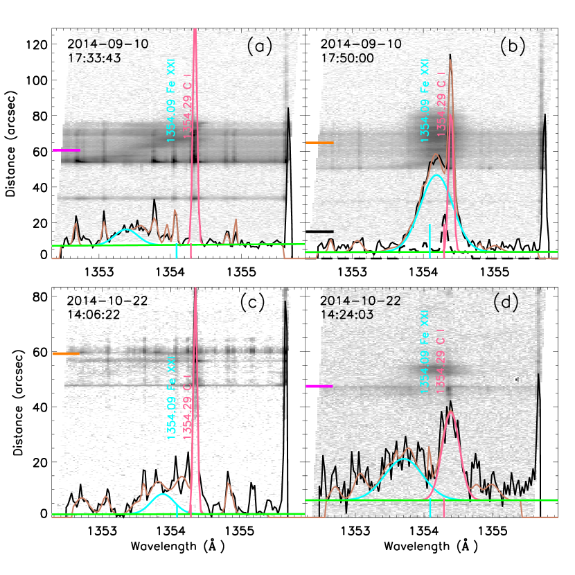
Figure 4: Similar as Fig. 3 (c), IRIS flare spectra at ‘O I ’ window at four time on 2014 September 10 and October 22, respectively. The black profiles are detected at various positions on the slit marked by the short horizontal lines. The brown profile represents the spectral fitting. The turquoise profile is Fe XXI , the magenta profile is C I , and the green is the background. The short vertical lines mark the rest wavelengths of Fe XXI (turquoise) and C I (magenta), respectively. The dashed black profile is the spectra from the non-flaring region.

Fig. 4 gives four examples of the multi-Gaussian fitting for the flares on 2014 September 10 (top) and October 22 (bottom), respectively. The short vertical lines represent the rest wavelengths of Fe XXI (turquoise) and C I (magenta). It is well known that Fe XXI is a hot coronal line with a formation temperature of about 11 MK (log T $\approx$ 7.05), which results into Fe XXI absent on the quiet Sun. Therefore, the rest wavelength of Fe XXI is not determined from the quiet regions. Recent studies from IRIS observations show that Fe XXI has a rest wavelength range between 1354.08 and 1354.10 Å (e.g., Tian et al., 2014a, 2015; Young et al., 2015; Graham & Cauzzi, 2015; Polito et al., 2015). In this paper, we use their average value of 1354.09 Å as Fe XXI rest wavelength. C I is a typical chromospheric line with a formation temperature of around 10⁴ K (log T $\approx$ 4.0) (Huang et al., 2014), and its rest wavelength can be determined from the emissions at the quiet regions, as the dashed profile shown in Fig. 4 (b), which plots the spectral profile average with 10 pixels around the position marked by the short black line. The spectra between 1353.66 Å and 1354.68 Å around C I are shown. In this paper, C I has a rest wavelength around 1354.29 Å.

2.3 Fitting parameters

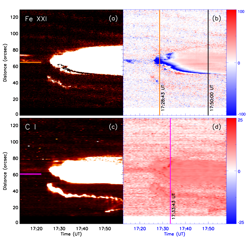
Figure 5: The space-time diagrams of intensities and Doppler velocities of Fe XXI and C I for the 2014 September 10 flare. Y-axis is the distance along the whole IRIS slit. The spectral profiles at two positions on the slit marked by short horizontal lines and three times marked by vertical lines are shown in Figs. 3 and 4 (a, b)

Using the method mentioned above, the intensities, line centers and widths of Fe XXI and C I can be determined from the multi-Gaussian fitting along the IRIS slit. Fig. 5 shows the space-time diagrams of the intensities (a, c) and Doppler velocities (b, d) of Fe XXI and C I from 17:12 to 17:58 UT for the 2014 September 10 flare. There are strong EUV line emissions at about 60″ $-$ 80″ and 35″ $-$ 40″ along the slit. These two regions correspond to two propagation fronts (around 120 arcsec and 100 arcsec along the slit at 17:26 UT) of the curved ribbon in Fig. 2 (b), and the north region is the flare ribbon marked by the arrow. The spectral profiles at two positions of 64.7″ and 60.6″ on the slit but three different time are given in Figs. 3 and 4 (a, b). The 2014 September 10 flare ribbon starts to cross IRIS slit at about 17:25 UT although there are weak emissions from 17:12 UT. The flare ribbon front displays a narrow point at the beginning, then expands rapidly to a wide range of $\sim$25″ after 17:40 UT along the slit. As mentioned before, this process suggests the flare ribbon propagation across the IRIS slit.

Doppler velocity is detected by the fitting line center separation from the rest wavelength, whatever Fe XXI or C I . Fig. 5 (b) shows that the flare ribbon starts blue shifts, then red shifts at coronal line of Fe XXI , which is due to the chromospheric evaporation at the beginning of the flare, then the hot materials fall back to the chromosphere along the flare loop after cooling. This is consistent with the standard flare model and previous findings (Czaykowska, 1999; Li & Ding, 2004), and the evaporation appears at the outer edge of the flare ribbon. On the other hand, the evaporation tends to appear at the front of flare ribbon. The evaporation speed can reach $\sim$230 km s^-1, while the falling speed is $\sim$25 km s^-1 in the corona. Fig. 5 (b) shows that the evaporation roughly has a time scale of more than 10 minutes. Fig. 5 (d) gives the space-time diagram of C I Doppler velocities. Different from coronal line of Fe XXI , the chromospheric line of C I exhibits red shifts all during the flare, indicating that the 2014 September 10 flare is the explosive evaporation. There is a velocity peak of C I at the same time as Fe XXI blue shift. The velocity can reach $\sim$27 km s^-1. After blue shift, Fe XXI displays the similar value of red shift as C I .

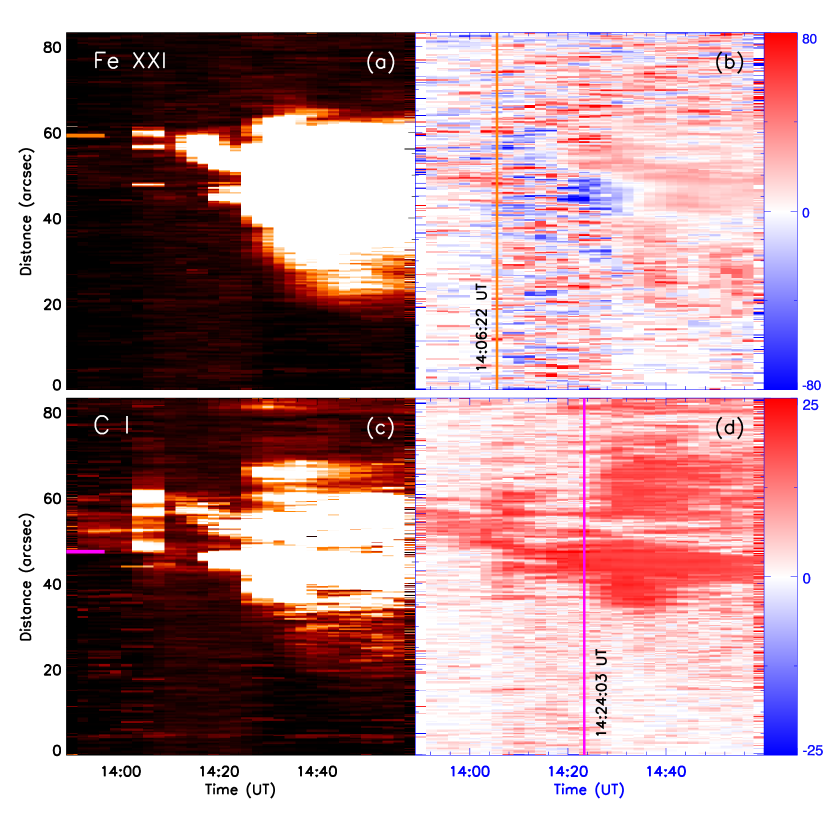
Figure 6: Same as Fig. 5, but for the 2014 October 22 flare. Y-axis gives the distance between two short blue lines along the IRIS slit in Fig. 1 (c, d). The spectral profiles at two positions on the slit marked by short horizontal lines and two times marked by vertical lines are given in Fig. 4 (c, d).

Same as Fig. 5, Fig. 6 gives the space-time diagrams along the IRIS slit of the intensities and Doppler velocities of Fe XXI and C I for the 2014 October 22 flare. As noted earlier, this event is observed in ‘raster’ mode with 8 steps. Thus, we can get 8 space-time diagrams at 8 step positions, respectively. Fig. 6 just shows the space-time diagram at the second step. In this case, the slit cadence is $\sim$131 (16.4$\times$8) s. The spectral profiles at two positions of about 59.2″ and 47.4″ on the slit are shown in Fig. 4 (bottom). Similar to the 2014 September 10 flare, this event is the explosive evaporation. The coronal line of Fe XXI displays blue shift at the ribbon onset, then red shift, while the chromospheric line of C I exhibits red shift during the whole flare. The evaporation speed can reach $\sim$145 km s^-1, and the falling speed is around 20 km s^-1. The evaporation timescale is roughly estimated more than 10 minutes.

3 Results

In order to study the relationship between the HXR emission and the evaporation speed, Fig. 7 plots the X-ray light curves and the time evolution of Doppler velocities at Fe XXI and C I for both events. The 2014 September 10 flare is well detected by Fermi, but missed by RHESSI, which detects the 2014 October 22 flare. Fig. 7 (a) shows the GOES 1.0$-$8.0 Å flux (black dashed lines) and Fermi/GBM light curves at 5 energy channels, such as 4.6$-$12.0 keV, 12.0$-$27.3 keV, 27.3$-$50.9 keV, 50.9$-$102.3 keV, and 102.3$-$296.4 keV. They are detected by the n2 detector, whose direction angle to the Sun is stable ($\sim$60^∘) before 17:45 UT, then its angle changes to the Sun to produce an X-ray peak, which is not real. There is a data gap after 17:54 UT. The time resolution of Fermi is 0.256 s, but becomes a higher value (0.064 s) automatically in the flare state. We rebin all the data into an uniform resolution of 0.256 s here, as shown in Fig. 7 (a). Fig. 7 (c, e) gives the time evolution of Fe XXI and C I Doppler velocities at two positions along the slit, i.e., at slit positions of 64.7″ (orange) and 60.6″ (purple) in Fig. 3 and 4 (upper). As predicted by the explosive evaporation, the coronal line of Fe XXI exhibits the blue shifts, while the chromospheric line of C I displays the red shifts at the same interval. Fe XXI increases its blue shifts rapidly to the maximum, then gradually and monotonically decreases to zero, continuously turns towards the red shifts. There are two possible explanations for these red shifts. Firstly, they maybe due to the hot material falling to the chromosphere along the flare loop after cooling. Secondly, they could be the signatures of loop contracting as seen in many imaging observations of flare arcades (e.g., Wang, 1992; Ambastha et al., 1993; Sui & Holman, 2003; Li & Gan, 2005, 2006; Ji et al., 2006, 2007; Zhou & Ji, 2009; Liu et al., 2013; Ning, 2013; Yan et al., 2013; Zhou et al., 2013; Kushwaha et al., 2015; Wang & Liu, 2015). Similar to Fe XXI , C I increases its red shifts firstly to the maximum and then decreases to a stable state of about 24 km s ^-1. There are two different physical scenarios to explain C I red shifts. The explosive peak of C I red shifts could be due to chromospheric condensation corresponding the evaporation detected as Fe XXI blue shifts at the same intervals, while the red shifts of C I on the decay phase could be due to the material falling back to chromosphere or the loop contracting, which results into the red shifts, not explosive but stable. Fe XXI and C I show explosive peak at the Doppler velocities, and the peak values can reach about -200 km s^-1 and 27 km s^-1, respectively. Although the peak time is different from the positions on the slit, the Doppler velocities exhibit the similar explosive peak. This is because the flare ribbon expands with time. The dashed lines in Fig. 7 (c) give the three times of the standard deviation (3$\sigma$) of the Doppler velocities from the quiet intervals (black profiles). The pluses (‘+’) mark the points where the speed values above 3$\sigma$ and corresponding to the HXR peaks. Here, the evaporation time scale can be estimated from Fe XXI blue shifts. It is about 10 minutes for the 2014 September 10 flare, which is consistent with recent findings for the same flare (Graham & Cauzzi, 2015; Tian et al., 2015). The pluses in Fig. 7 (e) mark the same points as that in Fig. 7 (c). After the blue shifts, Fe XXI becomes red shifts with a value of $\sim$24 km s^-1. Meanwhile, C I red shift velocity has the similar value ($\sim$24 km s^-1), indicating the material falling downward with a similar speed from the corona. The error bars of the multi-Gaussian fitting are displayed every 20-point with 2-$\delta$ uncertainties in Fig. 7 (c, e). The orange and purple colors are for two different positions on the slit, respectively. On the flare ribbon, the enhancement emissions result into the fitting speed errors decreasing to about 2 km s^-1 (i.e., $\delta$ = $\sim$2 km s^-1). Same as Fig. 7 (a, c, and e), Fig. 7 (b, d, and f) shows the light curves of X-ray, Fe XXI , and C I Doppler velocities for 2014 October 22 flare, which is well detected by RHESSI. As mentioned before, this event is detected by IRIS in ‘raster’ mode, and Fig. 7 (d and f) shows the Doppler velocities at the position of the second step in each raster. Same as Fig. 6, the time resolution is as low as 131 s. And the evaporation time scale of $\sim$11 minutes is estimated from Fe XXI blue shifts. The error bars of the multi-Gaussian fitting are shown by every 2-point for each Doppler velocity.

Fig. 7 (a) shows that there are three impulsive HXR peaks ($\geq$ 27.3 keV) as marked by ‘1’, ‘2’, and ‘3’. It is clear that the last two HXR peaks (‘2’ and ‘3’) are well correlated with the Doppler velocity peaks at two distinct positions, as shown in Fig. 7 (c, e), whatever Fe XXI or C I . In other words, both Fe XXI and C I exhibit a ‘increase-peak-decrease’ pattern of their Doppler velocities, well correlated with the ‘rising-maximum-decay’ phase at HXR emission. Considering the velocity direction, HXR light curves are anti-correlated with Fe XXI Doppler velocities, while correlated with C I Doppler velocities. This situation is well seen in the 2014 October 22 flare as well. There are two HXR peaks at the channel of 25$-$50 keV, as marked by ‘1’ and ‘2’ in Fig. 7 (b). They are well correlated with the Fe XXI and C I Doppler velocity peaks at two distinct positions, as shown in Fig. 7 (d, f).

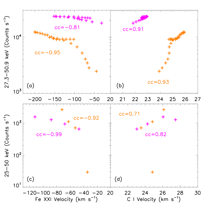
Figure 8: Scatter plots of two HXR peaks (orange and purple) dependence on Doppler velocities of Fe XXI and C I for the 2014 September 10 (a, b) and October 22 flares (c, d). The correlation coefficients (cc) are given.

Fig. 8 plots HXR peaks at 27.3$-$50.9 (or 25$-$50) keV dependence on the Fe XXI and C I Doppler velocities for the 2014 September 10 and 2014 October 22 flares, respectively. As expected from the electron-driven evaporation model, we find an anti-correlation between HXR emissions and coronal line (Fe XXI ) evaporation velocities, while correlation between HXR emissions and chromospheric line (C I ) condensation velocities. The correlation coefficient above 0.7 indicates that the non-thermal electrons cause the HXR emissions and drive the explosive evaporation simultaneously after precipitating in the chromosphere. Fig. 8 (c, d) shows only 4 points used for the correlation of each HXR peak due to the low time resolution of IRIS raster for the 2014 October 22 flare. For the peak ‘1’, the HXR emission at 25$-$50 keV starts an intensity as small as about 20 counts s^-1, then becomes more than one order bigger after the maximum. That results into a single point at about 20 counts s^-1 of HXR emission in Fig. 8 (c, d). The correlation coefficient will become larger if this point is omitted.

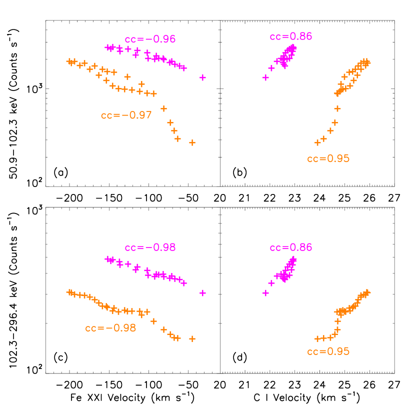
Figure 9: Same as Fig. 8, but HXR emissions at 50.9$-$102.3 keV and 102.3$-$296.4 keV for 2014 September 10 flare.

Fig. 9 plots the two HXR peaks at higher energy channels (such as 50.9$-$102.3 keV, and 102.3$-$296.4 keV) dependence on Fe XXI and C I Doppler velocities for the 2014 September 10 flare. The similar anti-correlation between HXR emissions and coronal line (Fe XXI ) Doppler shifts, while correlation between HXR emissions and chromospheric line (C I ) Doppler shifts are found during the same interval. The higher correlation coefficients ($>$ 0.85) further confirm our results.

4 Discussions

Using IRIS spectral observations on the flare ribbon and HXR observations from Fermi or RHESSI, we investigate the relationship between HXR emissions and Doppler velocities during the explosive evaporations in two X-class solar flares on 2014 September 10 and October 22. Using the multi-Gaussian fitting, Doppler velocities of Fe XXI and C I are detected from IRIS spectral observations. At certain position on the slit, Fe XXI and C I display their Doppler velocities with a ‘increase-peak-decrease’ pattern, which is well related to the ‘rising-maximum-decay’ phase of HXR emissions. Consistent with previous findings (Fisher et al., 1985a, b; Milligan & Dennis, 2009; Brosius, 2013; Tian et al., 2014a), we find a high anti-correlation between HXR emissions and coronal line Doppler shifts of Fe XXI , and a high correlation between HXR emissions and chromospheric line Doppler shifts of C I , indicating the electron beam-driven explosive evaporation in these two solar flares. The similar results are also found in the recent paper by Tian et al. (2015), who get a high correlation between Fe XXI blue shifts and derivative of GOES SXR for the 2014 September 6 and 10 flares.

As noted earlier, Fig. 7 plots the Fe XXI and C I Doppler velocities at two distinct positions respectively, which results into a good correlation with HXR peaks simultaneously. The peak time of Doppler velocities would be changed for various positions on the slit. In other words, Doppler velocities on the other positions are not well correlated with the HXR peaks at the same intervals. However, the time profiles of Doppler velocities at any positions exhibit the similar shape as shown in Fig. 7. We can still obtain the high correlations between Doppler velocities and HXR peaks after shifting an interval of Doppler velocity peaks. These intervals are different for the various positions along the slit, and it is an open question that a temporal correlation does not exist at these positions along the slit. Fig. 7 just gives the Doppler velocities at two special positions on the slit. They don’t need to shift with time to do the correlation in Figs. 8 and 9. For example, the first peak of the purple curve in Fig. 7 (e) is at 17:29 UT, and it could be correspond well with the peak ‘2’ in Fermi data if it is shifted an interval of about 1 minutes. While the second peak at 17:33 UT are corresponding well with the HXR peak ‘3’ without shifting. Tian et al. (2015) reported a time delay ($\sim$0.5$-$2.0 minutes) for the larger correlation between the Fe XXI blue shifts and SXR derivative on 2014 September 10 flare. This delay should be caused by the spectral profiles at different positions along the IRIS slit. When the flare ribbon propagates toward the South-West and expands with time, the peak of Fe XXI blue shifts changes with the slit positions, as well as with the time (seen in Figs. 2 and 5). In this paper, we fit all the spectra along the IRIS slit at all time to obtain the space-time images of Doppler velocities, and get the time evolution of Doppler velocities at any positions on the slit. On the other hand, both Fe XXI and C I exhibit red shifts on the flare decay phase, especially for the 2014 September 10 flare. As the cross (‘$\times$’) marked in Fig 7 (c, e), Fe XXI has a velocity of $\sim$24 km s^-1, while C I has a small peak. The spectral profile at this time is given in Fig. 4 (b), which shows strong emissions at Fe XXI and C I . At this position, Fe XXI and C I have line centers of about 1354.19 and 1354.40 Å, line widths of 524.33 mÅ and 76.96 mÅ. They show red shifts from their rest wavelengths. These red shifts of Fe XXI and C I could be caused by the material falling down or the loop contracting at the decay phase of the flares.

The rest wavelength of chromospheric line C I is set as 1354.29 Å, which is detected from the quiet Sun (seen in Fig. 4 (b)). This is consistent with recent studies from IRIS observations (Polito et al., 2015; Sadykov et al., 2015). However, as noted earlier, Fe XXI is a hot coronal line, which is absent on the quiet Sun. Therefore, we can not determine the rest wavelength of Fe XXI from non-flaring spectrum. There are different line centers of Fe XXI in the literatures. The first value of 1354.1 Å for Fe XXI has been identified from the spectra of solar flares by Doschek et al. (1975). Then the rest wavelength of Fe XXI is though between 1354.06 Å and 1354.12 Å (e.g., Cheng et al., 1979; Mason et al., 1986; Feldman et al., 2000; Innes et al., 2003a, b; Wang et al., 2003). In this paper, the rest wavelength of Fe XXI is set to 1354.09 Å, and this value is similar as that in recent studies (Tian et al., 2014a, 2015; Young et al., 2015; Graham & Cauzzi, 2015; Polito et al., 2015; Sadykov et al., 2015) about Fe XXI from IRIS spectral data. Considering the broad range of Fe XXI , the rest wavelength has an uncertainty of about $\pm$0.03 Å, corresponding the Doppler velocity of about $\pm$6.6 km s^-1. The rest wavelength of Fe XXI is probably taken from the decay phase of the flare due to it’s stable emission, as the example of the 2014 September 10 flare. However, the wavelength value is $\sim$1354.19 Å (i.e., the cross (‘$\times$’) in Fig. 7 (c, d)) at the decay phase of this flare, which is much bigger than the rest wavelength in previous studies. It is a fact that the coronal line of Fe XXI is absent in the non-flare regions where the temperature is not hot enough. Therefore, the intensities and Doppler velocities of Fe XXI in Figs. 5 (a, b) and 6 (a, b) outside the flare regions are invalid, they are fitting noises from the observation data. Same as the chromospheric line of C I , its Doppler velocities (Figs. 5 (d) and 6 (d)) outside the flare regions should also be fitting noises from the observation data.

The multi-Gaussian fitting is used to determine the Doppler velocities of Fe XXI and C I in this paper. There are three sources of uncertainties to their Doppler shifts. Firstly, as shown in Fig. 7, the fitting errors are very large in the non-flare regions and become much less in the flare regions, no matter Fe XXI or C I . This error is mathematic from the fitting method. Secondly, the red wing enhancement or redshifted component of the cool lines (i.e., Fe II , Si II , and C I ) could affect the identification of Fe XXI (Young et al., 2015; Tian et al., 2015). There is no way to exactly rule out these blending lines from Fe XXI at present time. Using tied intensities, line centers and widths could be a better approach as normally lines from the same ion or similar lines should have similar behaviors. Therefore, we constrained and tied these lines with the emission lines in other windows (seen in Table 1) to eliminate the influence of these cool lines. Thirdly, the asymmetries of C I line should also affect the derived red shift of C I . Because the Gaussian fitting of such asymmetrical lines tends to underestimate the velocity of chromospheric condensation, especially for the optically thick lines, i.e., Mg II line (Graham & Cauzzi, 2015), and H$\alpha$ line (Ding et al., 1995). A good way to determine the Doppler shifts from the asymmetric line is the bisector method (i.e., Ding et al., 1995; Graham & Cauzzi, 2015), which could accurately determine the Doppler shift, i.e., especially the red shift for the asymmetrical C I in our case. However, not the bisector, but the Gaussian fitting is used in this paper. Because C I is one of the multi-Gaussian fitting in our code, while the bisector method is a better way for the isolated line.

In this paper, we find the blue shifts of Fe XXI quickly increases from zero to the maximum (more than 200 km s^-1) before decreasing, which is different from Polito et al. (2015) finding that the evaporation speed shows a monotonic decrease once appearing at the flare ribbon. This would be because we take the whole history of the Fe XXI Doppler velocities during the impulsive phase of the flare, while Polito et al. (2015) only show the Doppler velocities after its maximum. On the other hand, their data is in ‘raster’ mode, rather than ‘sit and stare’ mode. The time resolution is not high. The 2014 October 22 flare in this paper is in ‘raster’ mode, and has a lower time resolution than the 2014 September 10 flare. But we can also detect the Doppler velocity increase before its maximum. The flare on 2014 September 10 is also studied by Graham & Cauzzi (2015); Tian et al. (2015). Both of them found very clearly monotonic decrease of the Fe XXI blue shifts, but no increase before the peak, as shown in Fig. 13 in Tian et al. (2015). They also found the evaporation within about 9 minutes, from 17:32 UT to 17:41 UT, which is similar to our finding of $\sim$10 minutes evaporation. From the orange curves in Fig. 7 (c), the start time of evaporation is about 17:26 UT (velocity above 3$\sigma$), and the end time is about 17:36 UT (velocity equally to zero), while the peak time is about 17:28 UT. Tian et al. (2015) showed the monotonic decrease of Fe XXI blue shifts for the 2014 September 10 flare after the maximum at 17:32 UT. Their velocity curve is at position around 117.8″on the slit. However, we give all the histories of the flare at the position of $\sim$64.7″along the slit in Fig. 7 (c), i.e., from the flare onset at 17:21 UT. On the other hand, Tian et al. (2015) found the same evaporation pattern of ‘increase-peak-decrease’ for 2014 September 6 flare when their fitting results cover the whole histories of the flare. In fact, previous studies had been reported the similar evolution of Doppler velocities from hot coronal lines (i.e., Fe XII , Fe XIX , Fe XXI , and so on) in the solar flares, such as the evolution of ‘increase-peak-decrease’ pattern (e.g., Wang et al., 2003; Kamio et al., 2005; Brosius, 2009; Raftery et al., 2009; Li et al., 2014; Tian et al., 2015). Fig. 7 (e) also shows that the chromospheric C I line seems to display several small peaks after its maximum. They could be related to the HXR emissions at the decay phase or the materials with various speeds falling back to chromosphere. Meanwhile, they probably are the spectral signatures of the various loop contracting.

Table 1: The parameters of 15 emission lines at three IRIS spectral windows.

IRIS window	Ion	Wavelength (Å)	Width (mÅ)	Intensity tied to
	Si II	1352.69$\pm$0.102	$\leq$ 260	Si II 1350.13
	Fe II	1353.07$\pm$0.051	$\leq$ 88	Fe II 1354.80
	Unknown	1353.40$\pm$0.061	$\leq$ 102	H2 1342.83
	Unknown	1353.61$\pm$0.061	$\leq$ 102	H2 1342.83
‘O I ’	Si II	1353.78$\pm$0.102	$\leq$ 260	Si II 1350.13
	Fe II	1354.06$\pm$0.051	$\leq$ 88	Fe II 1354.80
	Fe XXI	1354.09$\pm$1.28	$\geq$ 230
	C I	1354.29$\pm$0.26	$\leq$ 130
	Fe II	1354.80$\pm$0.051	$\leq$ 88
	Fe II	1354.91$\pm$0.061	$\leq$ 102
	Si II	1350.13$\pm$0.102	$\leq$ 260
	Unknown	1348.34$\pm$0.067	$\leq$ 102
‘Fe XII ’	Unknown	1348.60$\pm$0.067	$\leq$ 102
	Unknown	1349.65$\pm$0.051	$\leq$ 77
‘1343’	H2	1342.83$\pm$0.061	$\leq$ 102

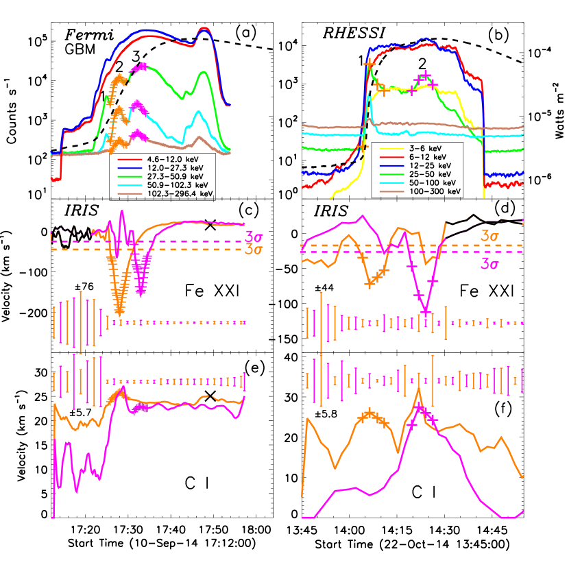
Figure 7: Top: the light curves from Fermi for the 2014 September 10 flare (a) and from RHESSI for the 2014 October 22 flare (b), and from GOES (dashed black lines) for both events. Middle and Bottom: the detected Doppler velocities of Fe XXI and C I at two distinct positions on the slits (seen text in details). The dashed lines are the three times of the standard deviation, the pluses (‘+’) mark the points with speed values above 3$\sigma$ and corresponding HXR peaks. The cross (‘$\times$’) marks the point in the decay phases of the flare, and its spectral profile is given in Fig. 4 (b). The error bars represent the 2-$\delta$ uncertainties from the multi-Gaussian fitting in the middle and bottom panels.

References

- Acton et al. (1982) Acton, L. W., & Leibacher, J. W., & Canfield, R. C., et al. 1982, ApJ, 263, 409
- Ambastha et al. (1993) Ambastha, A., Hagyard, M. J., & West, E. A. 1993, Sol. Phys., 148, 277
- Antonucci et al. (1982) Antonucci, E, & Gabriel, A. H., & Acton, L. W., et al. 1982, Sol. Phys., 78, 107
- Aschwanden & Benz (1995) Aschwanden, M. J., & Benz, A. O. 1995, ApJ, 438, 997
- Berlicki et al. (2005) Berlicki, A., & Heinzel, P., & Schmieder, B., et al. 2005, A&A, 430, 679
- Brosius & Holman (2007) Brosius, J. W., & Holman, G. D. 2007, ApJ, 659, L73
- Brosius (2009) Brosius, J. W. 2009, ApJ, 701, 1209
- Brosius (2013) Brosius, J. W. 2013, ApJ, 762, 133
- Brown (1971) Brown, J. C. 1971, Sol. Phys., 18, 489
- Brown (1973) Brown, J. C. 1973, Sol. Phys., 31, 143
- Carmichael (1964) Carmichael, H. 1964, NASA Special Publication, 50, 451
- Chen & Ding (2010) Chen, F., & Ding, M. D. 2010, ApJ, 724, 640
- Cheng et al. (1979) Cheng, C. C., & Feldman, U., & Doschek, G. A. 1979, ApJ, 233, 736
- Cheng et al. (2015) Cheng, X.,& Ding, M. D., & Fang, C. 2015, ApJ, 804, 82
- Czaykowska (1999) Czaykowska, A., & De Pontieu, B., & Alexander, D., & Rank, G. 1999, ApJ, 521, L75
- Curdt et al. (2001) Curdt, W., & Brekke, P., & Feldman, U., et al. 2001, A&A, 375, 591
- Curdt et al. (2004) Curdt, W., & Landi, E., & Feldman, U. 2004, A&A, 427, 1045
- De Pontieu et al. (2014) De Pontieu, B., & Title, A. M., & Lemen, J. R., et al. 2014, Sol. Phys., 289, 2733
- Del Zanna et al. (2006) Del Zanna, G., & Schmieder, B., & Mason, H., & Berlicki, A., & Bradshaw, S. 2006, Sol. Phys., 234, 95
- Ding et al. (1995) Ding, M. D., & Fang, C., & Huang, Y. R. 1995, Sol. Phys., 158, 81
- Ding et al. (1996) Ding, M. D., & Watanabe, T., & Shibata, K., et al. 1996, ApJ, 458, 391
- Doschek et al. (1975) Doschek, G. A., & Dere, K. P., & Sandlin, G. D., et al. 1975, ApJ, 196, L83
- Doschek et al. (1980) Doschek, G. A., & Feldman, U., & Kreplin, R. W., & Cohen, L. 1980, ApJ, 239, 725
- Doschek et al. (2013) Doschek, G. A., & Warren, H. P., & Young, P. R. 2013, ApJ, 767, 55
- Emslie et al. (1978) Emslie, A. G., & Brown, J. C., & Donnelly, R. F. 1978, Sol. Phys., 57, 175
- Falewicz et al. (2009) Falewicz, R., & Rudawy, P., & Siarkowski, M. 2009, A&A, 508, 971
- Feldman et al. (1980) Feldman, U., & Doschek, G. A., & Kreplin, R. W., & Mariska, J. T. 1980, ApJ, 241, 1175
- Feldman et al. (2000) Feldman, U., & Curdt, W., & Landi, E., & Wilhelm, K. 2000, ApJ, 544, 508
- Fisher et al. (1985a) Fisher, G. H, & Canfield, R. C., & McClymont, A. N. 1985a, ApJ, 289, 414
- Fisher et al. (1985b) Fisher, G. H, & Canfield, R. C., & McClymont, A. N. 1985b, ApJ, 289, 425
- Graham & Cauzzi (2015) Graham, D. R., & Cauzzi, G. 2015, ApJ, 807, L22
- Hirayama (1974) Hirayama, T. 1974, Sol. Phys., 34, 323
- Huang et al. (2014) Huang, Z., & Madjarska,M. S., & Xia, L., et al. 2014, ApJ, 797, 88
- Innes et al. (2003a) Innes, D. E., & McKenzie, D. E., & Wang, T. J. 2003a, Sol. Phys., 217, 267
- Innes et al. (2003b) Innes, D. E., & McKenzie, D. E., & Wang, T. J. 2003b, Sol. Phys., 217, 247
- Ji et al. (2006) Ji, H. S., & Huang, G. L., & Wang, H. M., et al. 2006, ApJ, 636, L173
- Ji et al. (2007) Ji, H. S., & Huang, G. L., & Wang, H. M. 2007, ApJ, 660, 893
- Ji et al. (2008) Ji, H. S., & Wang, H. M., & Liu, C., & Dennis, B. R. 2008, ApJ, 680, 734
- Kamio et al. (2005) Kamio, S., & Kurokawa, H., & Brooks, D. H., & Kitai, R., & UeNo, S. 2005, ApJ, 625, 1027
- Karlicky (1998) Karlicky, M. 1998, A&A, 338, 1084
- Kushwaha et al. (2015) Kushwaha, U., & Joshi, B., & Veronig, A. M., & moon, Y.-J. 2015, ApJ, 807, 101
- Kopp & Pneuman (1976) Kopp, R. A., & Pneuman, G. W. 1976, Sol. Phys., 50, 85
- Lemen et al. (2012) Lemen, J. R., & Title, A. M., & Akin, D. J., et al. 2012, Sol. Phys., 275, 17
- Li & Ding (2004) Li, J. P., & Ding, M. D. 2004, ApJ, 606, 583
- Li & Ding (2011) Li, Y., & Ding, M. D. 2011, ApJ, 727, 98
- Li et al. (2014) Li, Y., & Qiu, J., & Ding, M. D. 2014, ApJ, 781, 120
- Li & Zhang (2015) Li, T., & Zhang, J. 2015, ApJ, 804, L8
- Li et al. (2015) Li, D., & Ning, Z. J., & Zhang, Q. M. 2015, 2015, ApJ, 807, 72
- Li & Gan (2005) Li, Y. P., & Gan, W. Q. 2005, ApJ, 629, L137
- Li & Gan (2006) Li, Y. P., & Gan, W. Q. 2006, ApJ, 644, L97
- Lin et al. (2002) Lin, R. P., & Dennis, B. R., & Hurford, G. J., et al. 2002, Sol. Phys., 210, 3
- Liu et al. (2006) Liu, W., & Liu, S. M., & Jiang, Y. W., et al. 2006, ApJ, 649, 1124
- Liu et al. (2013) Liu, W., & Chen, Q., & Petrosian, V. 2013, ApJ, 767, 168
- Mason et al. (1986) Mason, H. E., & Shine, R. A., & Gurman, J. B., & Harrison, R. A. 1986, ApJ, 309, 435
- Meegan et al. (2009) Meegan, C., & Lichti, G., & Bhat, P. N., et al. 2009, ApJ, 702, 791
- Milligan et al. (2006a) Milligan, R. O., & Gallagher, P. T., & Mathioudakis, M., et al. 2006a, ApJ, 638, L117
- Milligan et al. (2006b) Milligan, R. O., & Gallagher, P. T., & Mathioudakis, M., et al. 2006b, ApJ, 642, L169
- Milligan & Dennis (2009) Milligan, R. O., & Dennis, B. R. 2009, ApJ, 699, 968
- Milligan et al. (2014) Milligan, R. O., & Kerr, G. S., & Dennis, B. R., et al. 2014, ApJ, 793, 70
- Milligan (2015) Milligan, R. O. 2015, arXiv:1501.04829
- Ning et al. (2009) Ning, Z. J., & Cao, W. D., & Huang, J., et al. 2009, ApJ, 699, 15
- Ning & Cao (2010) Ning, Z. J., & Cao, W. D. 2010, ApJ, 717, 1232
- Ning (2011) Ning, Z. J. 2011 Sol. Phys., 273, 81
- Ning & Cao (2011) Ning, Z. J., & Cao, W. D. 2011, Sol. Phys., 269, 283
- Ning (2013) Ning, Z J. 2013, Ap&SS, 346, 307
- Nitta et al. (2012) Nitta, S., & Imada, S., & Yamamoto, T. T. 2012, Sol. Phys., 276, 183
- Polito et al. (2015) Polito, V., & Reeves, K. K., & Del Zanna, G., & Golub, L., & Mason, H. E. 2015, ApJ, 803, 84
- Raftery et al. (2009) Raftery, & C. L., & Gallagher, P. T., & Milligan, R. O., & Klimchuk, J. A. 2009, A&A, 494, 1127
- Sadykov et al. (2015) Sadykov, V. M.,& Vargas Dominguez, S., & Kosovichev, A. G., et al. 2015, ApJ, 805, 167
- Schou et al. (2012) Schou, J., & Scherrer, P. H., & Bush, R. I., et al. 2012, Sol. Phys., 275, 229
- Sturrock (1966) Sturrock, P. A. 1966, Nature, 211, 695
- Sui & Holman (2003) Sui, L. H., & Holman, G. D. 2003, ApJ, 596, L251
- Syrovatskii & Shmeleva (1972) Syrovatskii, S. I., & Shmeleva, O. P. 1972, Soviet Ast., 16, 273
- Teriaca et al. (2006) Teriaca, L., & Falchi, A., & Falciani, R., & Cauzzi, G., & Maltagliati, L. 2006, A&A, 455, 1123
- Tian et al. (2014a) Tian, H., & Li, G., & Reeves, K. E., et al. 2014a, ApJ, 797, L14
- Tian et al. (2014b) Tian, H., & DeLuca, E., & Reeves, K. K., et al. 2014b, ApJ, 786, 137
- Tian et al. (2015) Tian, H., & Young, P. R., & Reeves, K. K., et al. 2015, arXiv:1505.02736
- Veronig et al. (2010) Veronig, A. M., & Rybák, J., & Gömöry, P., et al. 2010, ApJ, 719, 655
- Wang et al. (2003) Wang, T. J., & Solanki, S. K., & Curdt, W., et al. 2003, A&A, 406, 1105
- Wang (1992) Wang, H. M. 1992, Sol. Phys., 140, 85
- Wang & Liu (2015) Wang, H. M., & Liu, C. 2015, Research in Astronomy and Astrophysics, 15, 145
- Wülser et al. (1994) Wülser, J. P., & Canfield, R. C., & Acton, L. W., et al. 1994, ApJ, 424, 459
- Yan et al. (2013) Yan, X. L., & Pan, G. M., & Liu, J. H., et al. 2013, AJ, 145, 153
- Young et al. (2015) Young, P. R., & Tian, H., & Jaeggli, S. 2015, ApJ, 799, 218
- Zhang & Ji (2013) Zhang, Q. M., & Ji, H. S. 2013, A&A, 557, L5
- Zhou & Ji (2009) Zhou, T. H., & Ji, H. S. 2009, Research in Astronomy and Astrophysics, 9, 323
- Zhou et al. (2013) Zhou, T. H., & Wang, J. F., & Li, D., et al. 2013, Research in Astronomy and Astrophysics, 13, 526